On the Threshold of Drop Fragmentation under Impulsive Acceleration

Abstract

We examine the complete landscape of parameters which affect secondary breakup of a Newtonian droplet under impulsive acceleration. A Buckingham-Pi analysis reveals that the critical Weber number $(\mathit{We}_{cr})$ for a non-vibrational breakup depends on the density ratio $(\rho)$, the drop $(\mathit{Oh}_{d})$ and the ambient $(\mathit{Oh}_{o})$ Ohnesorge numbers. Volume of fluid (VOF) multiphase flow simulations are performed using Basilisk to conduct a reasonably complete parametric sweep of the non-dimensional parameters involved. It is found that, contrary to current consensus, even for $\mathit{Oh}_{d}\leq 0.1$, a decrease in $\mathit{Oh}_{d}$ has a substantial impact on the breakup morphology, motivating plume formation, and in turn affecting $\mathit{We}_{cr}$. It is found that in addition to $\rho$ (which previous studies have explored), $\mathit{Oh}_{o}$ also affects the balance between pressure differences between a droplet’s pole and its periphery, and the shear stresses on its upstream surface, which ultimately dictates the flow inside the droplet. This behavior manifests in simulations through the observed pancake shapes and ultimately the breakup morphology (forward or backward bag). All factors that play an essential role in droplet deformation process are specified and theories explaining the observed results on the basis of these factors are provided. A $\mathit{We}_{cr}-\mathit{Oh}_{d}$ plot is provided to summarize all variations in critical Weber number observed due to changes in the involved non-dimensional parameters. All observed critical pancake and breakup morphologies are summarized using a phase diagram illustrating all deformation paths a droplet might take under impulsive acceleration. Finally, based on the understanding of process of bag breakup gained from this work, a non-dimensional parameter to predict droplet breakup threshold is derived and tested on all simulation data obtained from this work and all experimental data gathered from existing literature.

1 Introduction

Droplet fragmentation, also known as secondary atomization, is the process of breakup of a droplet under the action of aerodynamic forces applied by the ambient flow. These forces originate due to a velocity deficit between the droplet and the ambient medium. There are two fundamental ways a droplet might experience a velocity deficit: a uniform ambient flow impacts a stationary droplet in a gravity-free environment, called “impulsive acceleration” (Han & Tryggvason, 2001); or an initially stationary droplet accelerates solely under the action of a constant body force, in the process also experiencing aerodynamic forces, called “free-fall” (Jalaal & Mehravaran, 2012). A liquid drop in both these cases experiences aerodynamic forces which leads to its deformation and might lead to breakup if its Weber number $\mathit{We}_{0}$ (3) exceeds a critical value $\mathit{We}_{cr}$ (Hinze, 1949, 1955) (7b). However, the physics accompanying free-fall and impulsive acceleration of droplets are very different from each other. During free-fall, the droplet starts with zero aerodynamic forces (zero velocity deficit) which gradually increase to a maximum as the droplet free falls, at either its terminal or its breakup velocity (if the droplet breaks up before reaching its terminal state). On the other hand, an impulsively accelerated droplet starts its deformation process with the largest velocity deficit, and correspondingly large aerodynamic stresses acting on its surface. These stresses gradually reduce as the droplet decelerates with respect to the ambient flow. It should be noted that the droplet as it decelerates, also simultaneously deforms causing an increase in its frontal area, which can in turn increase surface stresses, given the velocity deficit is still substantial. Hence, the $\mathit{We}_{cr}$ values corresponding to the the two cases are different.

Most industrial applications such as Internal Combustion Engines and spray painting involve impulsive acceleration type secondary atomization. A relevant setting where free-fall atomization might be important is aerial firefighting using fire retardants, or rainfall. Among impulsive acceleration cases, there can be different experimental systems such as a droplet introduced to a uniform cross-flow, or a droplet exposed to a shockwave in a wind tunnel (Hsiang & Faeth, 1992, 1995). Since the timescales of impulsive droplet breakup process is extremely small, both these systems behave similarly and show similar critical values.

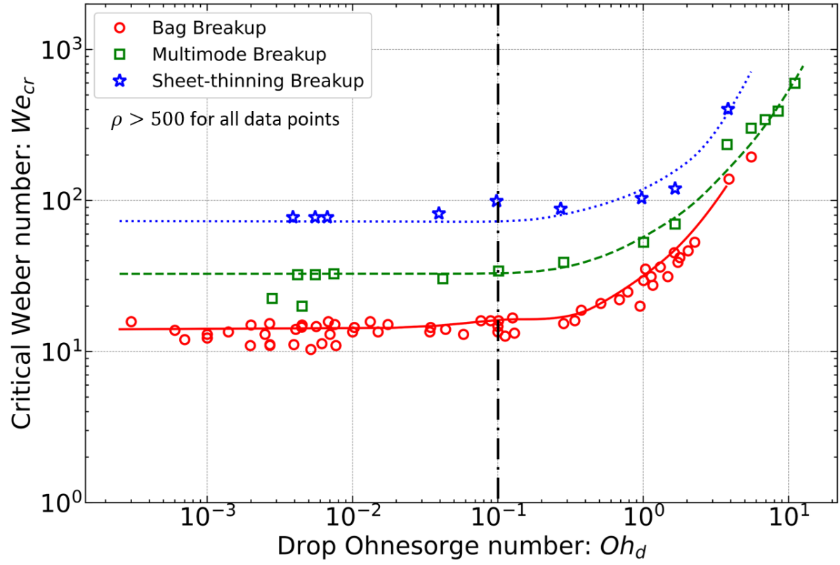
Figure 1: Plot aggregating all experimental data on Critical Weber number, based on a similar plot in Hsiang & Faeth (1995) and data from Krzeczkowski (1980); Pilch & Erdman (1987); Wierzba (1990); Dai & Faeth (2001); Guildenbecher et al. (2009); Kulkarni & Sojka (2014); Jackiw & Ashgriz (2021); Han & Tryggvason (2001); Jain et al. (2019).

Several experimental works have been conducted on secondary atomization (Pruppacher & Beard, 1970; Krzeczkowski, 1980; Wierzba, 1990; Hsiang & Faeth, 1992; Gelfand, 1996; Theofanous et al., 2004; Szakáll et al., 2009; Jain et al., 2015; Kulkarni & Sojka, 2014), however most of them focus on impulsive acceleration cases. This is due to the costs involved in conducting properly controlled free-fall experiments, which far exceed those involved in impulsive acceleration cases, due to the orders of magnitude larger timescales and lengthscales involved in the former. This timescale and lengthscale disparity also results in much larger computational costs associated with numerical simulations of free-fall. Owing to these reasons, for this work which involves a large number of numerical simulations, only impulsive acceleration cases have been focused upon.

Any further discussion on droplet deformation and breakup from this point forward focuses solely on impulsive acceleration mechanism.

Almost all droplets start their deformation process with flattening of its downstream face under the action of primarily pressure forces (Villermaux & Bossa, 2009; Jain et al., 2019; Jackiw & Ashgriz, 2021). This is followed by the formation of a pancake of one of the following two types: (a) a flat disk like structure with both upstream and downstream faces showing an increase in radius of curvatures (henceforth called “flat pancake”); or (b) a pancake with concave-shaped downstream surface, corresponding with minimal change in curvature of the upstream surface (henceforth called “forward pancake”) (Han & Tryggvason, 2001). These differences in pancake shapes have been observed for differences in rheological and flow parameters such as Density Ratio $\rho$ (7a), Initial Reynolds number $\mathit{Re}_{0}$ (or Outside Ohnesorge number $\mathit{Oh}_{o}$) (7c) and Drop Ohnesorge number $\mathit{Oh}_{d}$ (7d). However, the exact physical mechanism leading to this difference in pancake morphology has not yet been explored in literature. Beyond the formation of a pancake, the pancake deforms further and starts forming a toroidal periphery (rim), which then leads to further deformation and even possibly breakup of different morphologies (discussed in the next paragraph). This stage, which marks the completion of pancake formation and the start of a visible peripheral rim, can be temporally indicated through a non-dimensional time $t^{*}=t/\tau\approx 1$ (2). This non-dimensional time is scaled using a Deformation timescale $\tau$ (1) as derived by Rimbert et al. (2020). This timescale is the same as the dimensionless time for Rayleigh-Taylor or Kelvin-Helmholtz instabilities specified by Pilch & Erdman (Pilch & Erdman, 1987). $\tau$ includes the effect of $\rho$ on deformation timescale, thus making $t^{*}$ a useful temporal scale when comparing cases with different density ratios.

$$\tau=\frac{D}{V_{0}}\sqrt{\rho}$$ (1)

$$t^{*}=t/\tau$$ (2)

Here $V_{0}$ is the uniform initial velocity of the ambient medium relative to the droplet for an impulsive acceleration secondary atomization. $D$ is the volume averaged diameter of the droplet (or the diameter corresponding to its initial spherical shape). $t$ represents the real (simulation) time for the deformation process.

Following the formation of a pancake after $t^{*}>1$, the droplet may further deform and ultimately breakup through one the the following morphologies: (a) Vibrational mode where the drop oscillates about a maximum deformation state, and does not show consistent breakup (Hsiang & Faeth, 1992; Rimbert et al., 2020); (b) Simple Bag Breakup which involves the formation of a toroidal rim and the inflation of a thin film (bag) in between, which ultimately ruptures due to Rayleigh-Plateaus instabilities (Kulkarni & Sojka, 2014; Jackiw & Ashgriz, 2021); (c) a bag breakup with morphological features in addition to a bag, such as stamen/plume (Hsiang & Faeth, 1995; Jain et al., 2015) or multiple bags (Cao et al., 2007; Jackiw & Ashgriz, 2021); (d) Sheet Thinning breakup where thin sheets and ligaments are removed from the periphery of the pancake, and are blown downstream relative to the droplet core due to their low local inertia, ultimately breaking up due to instabilities (Khosla & Smith, 2006; Guildenbecher et al., 2009); and (e) catastrophic breakup where unstably growing surface waves pierce through the entire pancake and cause it to catastrophically disintegrate (Theofanous, 2011).

In nature under standard atmospheric conditions, most liquid-air droplet-ambient systems have $\rho>500$, $\mathit{Oh}_{d}>0.001$, and $0.001<\mathit{Oh}_{o}<0.01$. For this limited parameter space, most experimentally observed critical droplet breakup morphologies have been simple bag breakups. On the other hand, most Direct Numerical Simulations (Han & Tryggvason, 2001; Jalaal & Mehravaran, 2014) until the recent advent of Petascale computing have covered low density ratios ($\rho<50$) due to computational limitations and lack of efficient adaptive mesh refinement algorithms. These simulations show a very different breakup process (e.g., forward pancake and bag formation) and critical Weber Number values compared to the experiments. This hints at the vital role played by density ratio in deciding droplet breakup threshold and specific breakup morphologies. Only recently, DNS for high $\rho$ droplets have become more common (Jain et al., 2015, 2019; Marcotte & Zaleski, 2019; Dorschner et al., 2020) and further emphasize the large role played by $\rho$ on the value of $\mathit{We}_{cr}$ as well as the threshold Weber number for the transition from bursting to stripping (Marcotte & Zaleski, 2019). Jain et al. (2019) explored the effect of $\rho$ on droplet deformation for a specific $\mathit{Re}_{0}$ and viscosity ratio for a range of $\mathit{We}_{0}$ from $20$ to $100$, and observed the immense impact $\rho$ has on bag and pancake orientation, droplet velocities and observed total deformations. Similar conclusions were reached by Marcotte & Zaleski (2019) with regards to the effect of density ratio on deformation morphology, with large $\rho$ cases showing higher incidences of plume (stamen) formation at the upstream pole of the droplet.

By 1990s, several experimental and theoretical works (Karam & Bellinger, 1968; Krzeczkowski, 1980; Pilch & Erdman, 1987) had established the important role played by $\mathit{Oh}_{d}$ in affecting the magnitude of $\mathit{We}_{cr}$ for a droplet-ambient system. This role was greatly expanded upon by Hsiang & Faeth’s review paper in 1995 (Hsiang & Faeth, 1995), where they aggregated all the experimental data from existing literature as well as their own experiments into $\mathit{We}_{cr}$ vs. $\mathit{Oh}_{d}$ plots. Their findings showed that that the threshold $\mathit{We}_{0}$ for the onset of all breakup morphologies (both simple backward bag and other higher $\mathit{We}_{0}$ breakup morphologies) follow the same trend with respect to $\mathit{Oh}_{d}$ (see figure 1 of Hsiang & Faeth (1995) or figure 1), with threshold $\mathit{We}_{0}$ being almost independent of $\mathit{Oh}_{d}$ values for $\mathit{Oh}_{d}<0.1$, and then increasing rapidly for $\mathit{Oh}_{d}>0.1$. Furthermore, Critical breakup morphology (for the onset of breakup) of all experimental cases were observed to be simple bag breakups. It is essential to note that all the observations made in Hsiang & Faeth (1995) were made on the previously specified experimentally feasible parameter space. Villermaux & Bossa (2009) was the first to analytically describe bag breakup process for an inviscid droplet and derived a constant threshold value of 6 for $\mathit{We}_{cr}$, an underestimation when compared to experimentally seen threshold values. Their work was extended to include droplet fluid viscosity, first by Kulkarni & Sojka (2014) and most recently by Jackiw & Ashgriz (2021), which resulted in a function of $\mathit{Oh}_{d}$ describing $\mathit{We}_{cr}$. This corrected the underestimation and lead to a great match with previous experimental results. The aforementioned analytical works had not taken into consideration the role of factors such as ambient viscosity ($\mathit{Oh}_{o}$) and density ($\rho$) (which in turn dictates droplet’s relative velocity with the ambient) in affecting droplet’s deformation characteristics. However, the density and viscosity contrasts between the ambient and the droplet fluids is normally substantial for experimental systems, which results in a good match with experimental $\mathit{We}_{cr}$ values, even when the aforementioned factors are not considered. However (as will be explored in detail in this work), for systems where the rheological contrast between the ambient and the droplet fluids is not substantial, these factors must be taken into consideration for correct estimation of threshold $\mathit{We}_{0}$ values.

The almost independence of droplet fragmentation threshold with respect to $\mathit{Oh}_{d}$ for $\mathit{Oh}_{d}<0.1$ as observed in most experimental works has an interesting side-effect: it has become a somewhat a common practice to assume a constant arbitrary $\mathit{Oh}_{d}$ value of less than $0.1$ for most analysis as a representative value for all low viscosity droplet breakups. Very few works hence exhaustively explore the effect of varying $\mathit{Oh}_{d}$ for $\mathit{Oh}_{d}<0.1$. One such work is that of Jain et al. (2019) where they explored the effect of viscosity ratio (and hence $\mathit{Oh}_{d}$) on breakup morphologies through simulations of droplets of $\rho=1000$ and two different viscosity ratios, and observed that the threshold $\mathit{We}_{0}$ values reduced with decreasing $\mathit{Oh}_{d}$. They also observed the appearance of a plume at the upstream pole for lower viscosity ratio cases for the same $\mathit{We}_{0}$.

Initial Reynolds number $Re_{0}$ (or alternatively Ambient Ohnesorge Number $\mathit{Oh}_{o}$) also remains to be exhaustively explored, especially in context of critical droplet breakup threshold. Han & Tryggvason (2001) did simulations for different $\mathit{Re}_{0}$ values for some low density ratio cases, and observed large reduction in droplet deformations for low $\mathit{Re}_{0}$ values. They speculated that this reduction in deformation might lead to a rise in $\mathit{We}_{cr}$ values. Very few other works have explored or commented on the impact of $\mathit{Oh}_{o}$ on droplet breakup (Guildenbecher et al., 2009; Jain et al., 2019; Marcotte & Zaleski, 2019). Jain et al. (2019) once again was one of the very few works to analyze the impact of $\mathit{Re}_{0}$ on high density ratio droplets ($\rho=1000$) and observed higher incidences of plume formation in backward bag morphology for higher $\mathit{Re}_{0}$ values.

Hence, there exists a space for a single cohesive study analyzing the effect of all the relevant non-dimensional parameters such as $\mathit{Oh}_{o}$, $\mathit{Oh}_{d}$, and $\rho$ on droplet deformation and breakup, and subsequently their impact on the threshold Weber numbers observed for critical breakup ($\mathit{We}_{cr}$). In this work, we explore the effect of each of these parameters computationally using an open-source solver “Basilisk”, for all combinations of the other parameters, i.e. perform a parametric sweep, so that the forces driving the droplet’s deformation and resulting internal flows can be understood. It should be noted that a distinction between liquid-gas and liquid-liquid droplet-ambient systems has been maintained in the currently existing literature. However fundamentally, the only differentiating factor between the two systems is the density and viscosity ratios, as well as the surface tension of the fluid interface. It is expected that the need for this distinction should vanish for a sufficiently large parameter space involving $\rho$, $\mathit{Oh}_{o}$ and $\mathit{Oh}_{d}$. Hence a large range of values of $\rho$ and $\mathit{Oh}_{o}$ are considered, so as to capture both liquid-liquid and liquid-gas systems. $\mathit{Oh}_{d}$ values explored in this work are restricted to $\mathit{Oh}_{d}\leq 0.1$, to restrict our focus on a parameter space less explored in literature. We start with a description of the relevant impulsive acceleration problem (section 2.1) and the numerical scheme and corresponding assumptions used for this work (section 2.2 and 2.3). The parameter space to be numerically explored is described in detail in section 2.4. The effect of each of $\mathit{Oh}_{d}$, $\mathit{Oh}_{o}$, and $\rho$ on droplet deformation given other parameters are constant, are described in detail, and connected to the forces and internal flow observed in the droplets (section 3). During the course of the parameter sweep, by simulating a range of Weber number values for every non-dimensional parameter set, the corresponding critical Weber number can be discovered. This should allow us to recreate the $\mathit{We}_{cr}$ vs. $\mathit{Oh}_{d}$ plot similar to figure 1 for all the threshold cases found through current simulations. Such a plot should illustrate the effect of each relevant non-dimensional parameter on the magnitude of $\mathit{We}_{cr}$ and corresponding critical breakup morphologies. Based on the insights gained from the simulations, a non-dimensional parameter can then be derived through a scaling analysis that incorporates the effects of all the relevant non-dimensional parameters, and conceivably describe the observed variations in threshold behavior of a droplet better than the commonly used characteristic critical fragmentation criteria $\mathit{We}_{cr}$.

2 Problem Description and implementation

2.1 Problem Description and Non-dimensionalisation

Let us consider a droplet of diameter $D$ containing a fluid of density $\rho_{d}$ and dynamic viscosity $\mu_{d}$ ( subscript $d$ implies properties associated with the droplet). It is impulsively accelerated by a uniform flow of density $\rho_{o}$ and viscosity $\mu_{o}$ ( subscript $o$ implies properties associated with the ambient medium, i.e. outside the droplet), with a uniform velocity $V_{0}$, starting at $t=0$. The surface tension of the droplet-ambient interface is $\sigma$. If we assume that $V_{0}$ is equal to the critical (lowest possible) velocity required for a non-vibrational breakup of the droplet, i.e. $V_{cr}$, the Weber number (3) corresponding to such a flow would be the critical Weber number $\mathit{We}_{cr}=(\rho_{o}V_{cr}^{2}D)/\sigma$. We would like to find all the non-dimensional parameters on which $\mathit{We}_{cr}$ depends. We can establish such a relationship using Buckingham-Pi Analysis:

$$\text{Initial Weber number: }\mathit{We}_{0} =\frac{\rho_{o}V_{0}^{2}D}{\sigma}$$ (3)

$$\text{Initial Reynolds number: }\mathit{Re}_{0} =\frac{\rho_{0}V_{0}D}{\mu_{o}}$$ (4)

$$\text{Instantaneous Reynolds number: }\mathit{Re} =\frac{\rho_{0}V_{\mathit{rel}}D_{\mathit{rel}}}{\mu_{o}}$$ (5)

$$V_{cr} =f\left(\rho_{o},\rho_{d},\mu_{o},\mu_{d},D,\sigma\right)$$ (6a)

$$\sqrt{\mathit{We}_{cr}} =f(1,\rho,\mathit{Oh}_{o},\mathit{Oh}_{d}\sqrt{\rho},1,1)$$ (6b)

$$\mathit{We}_{cr} =F\left(\rho,\mathit{Oh}_{o},\mathit{Oh}_{d}\right)$$ (6c)

We have the following definitions:

$$\text{Density Ratio: }\rho =\frac{\rho_{d}}{\rho_{o}}$$ (7a)

$$\text{Critical Weber number: }\mathit{We}_{cr} =\frac{\rho_{o}\,V_{cr}^{2}\,D}{\sigma}$$ (7b)

$$\text{Outside Ohnesorge number: }\mathit{Oh}_{o} =\frac{\mu_{o}}{\sqrt{\rho_{o}\,\sigma\,D}}=\frac{\sqrt{\mathit{We}_{0}}}{\mathit{Re}_{0}}$$ (7c)

$$\text{Drop Ohnesorge number: }\mathit{Oh}_{d} =\frac{\mu_{d}}{\sqrt{\rho_{d}\,\sigma\,D}}$$ (7d)

Hence, for an impulsively accelerated drop as previously defined, $\mathit{We}_{cr}$ in the most general sense is dependent on $\rho$, $\mathit{Oh}_{d}$ and $\mathit{Oh}_{o}$.

Weber number $\mathit{We}_{0}$ represents the competition between dynamic pressure forces driving the deformation of the droplet and the capillary forces resisting this deformation. Hence as $\mathit{We}_{0}$ is increased, the maximum deformation observed in the corresponding droplet increases, as long as $\mathit{We}_{0}$ remains less than $\mathit{We}_{cr}$, beyond which the droplet breaks up.

Density Ratio $\rho$ is a measure of droplet’s inertia compared to the ambient medium, and hence represents its acceleration in response to external forces. Dynamic pressure forces applied by the ambient medium scale with $\rho_{o}$ and hence their capability to induce accelerations in parts or whole of the droplet is inversely proportional to $\rho$.

Drop Ohnesorge number $\mathit{Oh}_{d}$ is a ratio of Capillary and Momentum Diffusion timescales (equation 14) and provides an estimate of how energy supplied to a droplet by the external forcing distributes across surface energy and viscous dissipation.

Ambient Ohnesorge number $\mathit{Oh}_{o}$ is a measure of ambient viscosity and provides a non-dimensional velocity independent analogue for initial Reynolds number $\mathit{Re}_{0}$ (equation 4).

Over the timescales over which a droplet deforms and fragments, it can experience significant centroid accelerations which necessitate consideration of its instantaneous Reynolds number as it changes during its deformation process. Hence, in addition to $\mathit{Re}_{0}$, we also define an instantaneous Reynolds number $\mathit{Re}$ (equation 5), which is based on its velocity deficit ($V_{\mathit{rel}}$) with the ambient medium, and its frontal radius of its deformed shape ($D_{\mathit{rel}}$).

We non-dimensionalize the problem parameters such that all the parameters are expressed on the basis of these non-dimensional numbers.

When $\rho_{o}$, $V_{0}$ and $D$ are taken as the basis variables for non-dimensionalisation; we can write the non-dimensional forms of the associated variables as follows:

$$\tilde{D} =\frac{D}{D}=1$$ (8a)

$$\tilde{V_{0}} =\frac{V}{V_{0}}\quad;\quad\therefore\tilde{V}_{0}=1$$ (8b)

$$\tilde{\rho}_{o} =\frac{\rho_{o}}{\rho_{o}}=1\quad;\quad\tilde{\rho_{d}}=\frac{\rho_{d}}{\rho_{o}}=\rho$$ (8c)

$$\tilde{\sigma} =\frac{\sigma}{\rho_{o}V_{0}^{2}D}=\frac{1}{\mathit{We}_{0}}$$ (8d)

$$\tilde{\mu}_{o} =\frac{\mu_{o}}{\rho_{o}V_{0}D}=\mathit{Oh}_{o}\sqrt{\frac{1}{\mathit{We}_{0}}}\quad;\quad\tilde{\mu}_{d}=\frac{\mu_{d}}{\rho_{o}V_{0}D}=\mathit{Oh}_{d}\sqrt{\frac{\rho}{\mathit{We}_{0}}}$$ (8e)

Hence, for a specific ambient-droplet fluid combination (i.e. fixed Rheological properties), a specific droplet diameter, and a specific inflow velocity, we get a set of $\{\rho,\mathit{Oh}_{o},\mathit{Oh}_{d},\mathit{We}_{0}\}$ which completely defines the system. A droplet under these conditions can then be simulated in Basilisk to test if it shows a non-vibrational breakup. If the droplet does not fragment, $\mathit{We}_{0}$ is increased (which can be attributed to a decrease in $\sigma$ in the non-dimensional space, or an increase in inflow velocity in dimensional space) and the impulsive acceleration simulation is rerun. These steps are repeated until the drop shows a non-vibrational breakup. The corresponding minimum $\mathit{We}_{0}$ marking the onset of non-vibrational breakup is the critical Weber number $\mathit{We}_{cr}$ for that non-dimensional parameter set.

2.2 Numerical scheme

The simulations have been performed using an open source solver suite ”Basilisk” (www.basilisk.fr). It is a set of open-source codes which can solve a variety of partial differential equations on adaptive cartesian meshes. Basilisk (and its predecessor ”Gerris”) has been extensively validated for various fundamental problems related to two phase flows (Popinet, 2003, 2009; Marcotte & Zaleski, 2019), and hence is the ideal tool to handle droplet simulations across a large range of $\rho$ and $\mu$ values. We use its Navier-Stokes Centered solver in conjunction with its two-phase flow formulation for simulating the droplets. Basilisk solves incompressible Navier Stokes multiphase flow equations (9 10 & 11) on a quad/octree discretized grid, which allows variable mesh densities at the interface (Popinet, 2003).

$$\rho(\partial_{t}\mathbf{u}+\boldsymbol{u}.\boldsymbol{\nabla u}) =-\boldsymbol{\nabla}p+\boldsymbol{\nabla}.(2\mu\boldsymbol{D})+\sigma\kappa\delta_{s}\boldsymbol{n},$$ (9a)

$$\partial_{t}\rho+\boldsymbol{\nabla}.(\rho\,\boldsymbol{u}) =0,$$ (9b)

$$\boldsymbol{\nabla.u} =0$$ (9c)

where $\boldsymbol{u}=(u,v,w)$ is the fluid velocity, $\rho\equiv\rho(\boldsymbol{x},t)$ is the fluid density, $\mu\equiv\mu(\boldsymbol{x},t)$ is the dynamic viscosity and $\boldsymbol{D}$ is the deformation tensor defined as $D_{ij}=(\partial_{i}u_{j}+\partial_{j}u_{i})/2$. The Dirac distribution function $\delta_{s}$ allows the inclusion of surface tension body force term in the one governing equation being solved in this scheme by switching on the surface tension term only at the interface between the fluids; $\sigma$ is the surface tension coefficient, $\kappa$ and $\boldsymbol{n}$ the curvature and normal to the interface respectively. $\kappa$ is calculated using Height Function (HF) formulation as described by Torrey et al. (1985), taking care to consider under-resolved interfaces. The surface tension term is calculated using Continuum Surface Force (CSF) approach first described in Brackbill et al. (1992), with special care taken to ensure that the conditions described in Francois et al. (2006) are satisfied to prevent parasitic currents.

To maintain the single equation formulation of the momentum equation, the two fluids are represented using a volume fraction $c(\boldsymbol{x},t)$ according to which $\rho$ and $\mu$ are defined as:

$$\rho =c\,\rho_{1}+(1-c)\,\rho_{2},$$ (10a)

$$\mu =c\,\mu_{1}+(1-c)\,\mu_{2}$$ (10b)

Here $\rho_{1},\rho_{2}$ and $\mu_{1},\mu_{2}$ are the densities of the first and second fluid in the domain respectively. In this formulation, the density advection equation is hence replaced with a volume fraction advection equation:

$$\partial_{t}c+\boldsymbol{\nabla}.(c\,\boldsymbol{u})=0$$ (11)

A Detailed description of the numerical scheme relevant for this work is presented in Popinet (2003, 2009).

A significant fraction of the simulations in this work involve high density ratios ($\rho>500$). For such high density ratios, a sharp interface can cause instabilities at the interface due to an unnatural spike in kinetic energy (Jain et al., 2015). The same has been observed in all our large $\rho$ simulations with low $\mathit{Oh}_{d}$ ($\mathit{Oh}_{d}\leq 0.001$) (not shown here), where the upstream face shows unnaturally large surface instabilities which leads to removal of micro-droplets from the main droplet. Hence, we smear the interface by using a vertex average of $c$ to reduce the density gradients across the interface. Using a smoothed field prevents premature breakup of the interface. The numerical scheme with this smearing will be validated for a high $\rho$ case in the next section.

The entire computational domain is discretized using squares for 2D (quadtree) and cubes for 3D (octree) and then organized in a hierarchy of cells. The mesh resolution is adaptive in nature, and hence the two-fluid interface can be resolved at a much higher resolution compared to other computationally less interesting parts of the domain. This allows for large savings in the computational costs for two-phase simulations. Any cell (parent computational element) can be further refined in to four or eight equal children cells for 2D and 3D computation respectively. Each of the children cells can themselves act as parent cells if required. This successive refinement goes on until a (user-defined) threshold criterion for error is satisfied, or a maximum refinement level is reached. A Wavelet based error estimation is used to estimate errors associated with the specified fields (Popinet, 2015) while the maximum allowed refinement (smallest allowed cell) is restricted by a specified minimum allowed cell dimension, which is defined by a parameter called “Maximum Level”. A Maximum level of $N$ corresponds to a minimum cell size of $L/2^{N}$.

This work requires a large number of simulations for the performance of a complete parametric sweep across the parameters specified in equation 6(c). Hence, 3D simulations are computationally not feasible. Furthermore, the process of deformation of a droplet under impulsive acceleration (and close to critical conditions) is axisymmetric in nature for the majority of the process, starting from the initial pancake formation until the inflation of the pancake into a bag. It is the final inflation of the expanding bag and the corresponding rupture, driven by interfacial instabilities, that cannot be assumed to be axisymmetric. The main focus of this work is characterizing the deformation morphologies achieved by a droplet during its deformation process and its final fate, i.e. whether the droplet breaks up and its general morphology right before breakup. The exact size of the fragmentation morphology or the final drop size distribution after fragmentation, which would require a fully resolved 3D DNS, are not information of importance for this work. Hence, for the purposes of this work, axisymmetric simulations are sufficient. The validity of this assumption of axisymmetry in the context of this work will be ensured in section 2.3.

The general simulation domain used for defining the simulations in this work is illustrated in figure 2. The domain is a square domain (for compatibility with quadtree meshes) of size L, chosen such that the droplet always remains sufficient distance away from the boundaries, at minimum a distance of $16D$ away from the droplet center. The top boundary is a symmetric boundary ($\partial_{n}P=\partial_{n}u_{t}=u_{n}=0$), the bottom boundary is the axisymmetry axis. The left boundary allows a uniform ambient fluid inflow into the domain ($u_{n}=V_{0}$), and the right boundary allows the flow to leave the domain freely ($\partial_{n}u_{n}=0$).

$\rho$	$\mathit{Oh}_{o}$	Velocity Jump ($\delta V$)
$10$	$0.1$	0.143
$50$	$0.1$	0.029
$100$	$0.1$	0.0147

Table 1: This table lists centroid velocity jumps seen for droplets of different $\rho$ values after the first timestep.

At t=0, the ambient fluid is quiescent, and a droplet with zero initial velocity is initialized some distance from the left boundary. Given the flow in the simulation is incompressible and any information in this domain travels at an infinite propagation speed, at the end of the $1^{st}$ timestep, the whole domain has achieved a flow velocity compliant with the left inflow boundary conditions. This involves obtaining an incompressible flow around the droplet. In real life, this process occurs in a finite amount of time dependent on the velocity of the acoustic wave velocity. However for a numerical system, this occurs in one timestep and leads to a jump in droplet centroid velocity, without gaining any corresponding deformation. The magnitude of this velocity jump in droplet’s centroid velocity ($\delta V$) is inversely proportional to $\rho$ (Marcotte & Zaleski, 2019). Hence, the effective relative velocity experienced by the droplet reduces to $V_{\mathit{eff}}=1-\delta V$. It becomes essential to take into consideration this effective velocity when calculating the associated $\mathit{We}_{0}$ of the system. For this purpose, a few simulations for each density ratio and different $\mathit{Oh}_{o}$ values were run, and the associated jump was used to calculate the effective $\mathit{We}_{0}$ and corresponding effective $\mathit{Oh}_{o}$ and $\mathit{Oh}_{d}$ values for each $\rho$. The obtained velocity jumps are summarized in table 1. $\rho=10$ shows a significant jump of approximately $0.14$, and $\rho=100$ shows a negligible jump of approximately $0.015$. All corresponding non-dimensional parameters as well as performed simulations have been corrected to incorporate this jump. For all $\rho>100$ simulations, this $1^{st}$ timestep jump is considered to be insignificant.

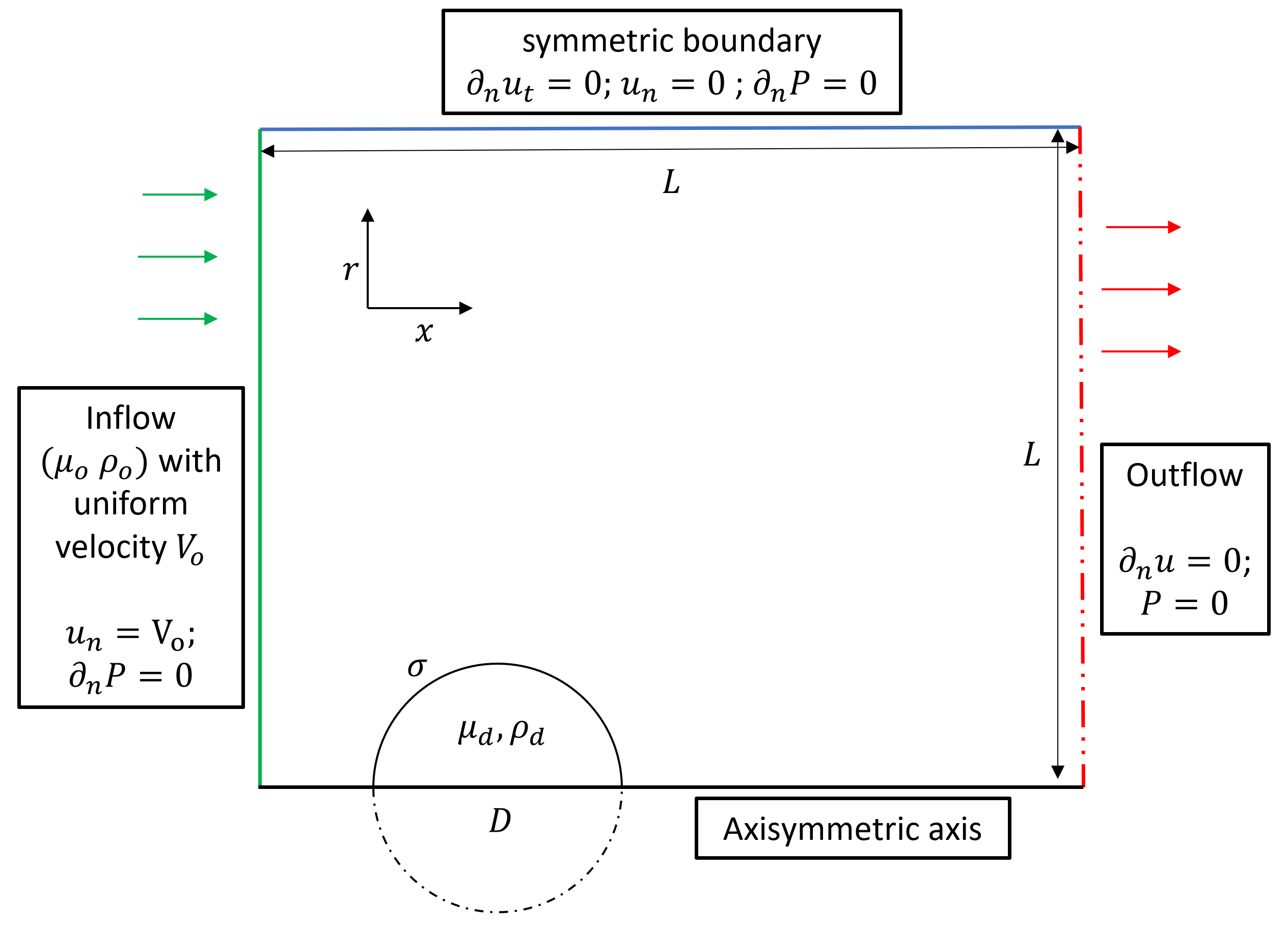
Figure 2: The axisymmetric domain used for all simulations in this work. At $t=0$, the simulation starts with a stationary axisymmetric spherical droplet under the action of an ambient flow of uniform velocity.

2.3 Validation of Axisymmetric numerical scheme

2.3.1 Test for Convergence

Before using Basilisk for the production runs, it is essential to test convergence of the numerical scheme with regards to both the maximum mesh resolution (normally achieved at the interface) and Wavelet-error thresholds for the specified field variables. For droplet simulations, the accuracy of the calculated interface and the velocity fields must be ensured for correct retrieval of surface stresses, and correspondingly droplet deformation and breakup. Hence, maximum allowed errors in velocity field ($u_{e}$) and volume fraction field ($c_{e}$) are specified to dictate the refinement algorithm. Additionally, a maximum allowed refinement level ($N$) is specified to constrain the adaptive mesh refinement from generating computational cells smaller then a specified resolution, so as to prevent very large number of computational cells, as well as extremely small simulation timesteps corresponding to the smallest cells.

To test the convergence of Basilisk with respect to these parameters, we simulate multiple cases with varying $u_{e}$, $c_{e}$ and $N$, and fixed physical properties of $\{\rho,\mathit{Oh}_{o},\mathit{Oh}_{d},\mathit{We}_{0}\}=\{500,0.01,0.1,16\}$ on an axisymmetric domain (figure 2) with $L=16$, $D=1$ and $V_{0}=1$. A case with these physical properties is expected to show a bag breakup and hence provides a good platform to test the convergence of these parameters at all deformation magnitudes. The corresponding convergence plots are shown in figure 3.

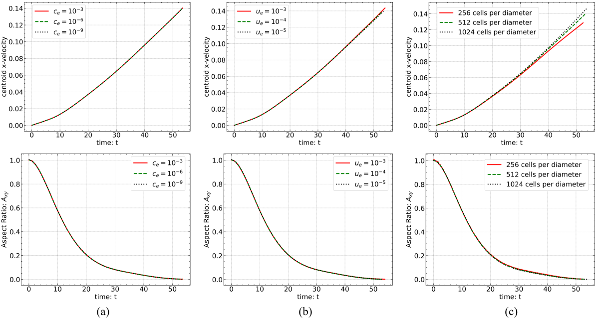
Figure 3: Tests of convergence plots for the choice of wavelet based error thresholds for (a) $c$ and (b) $\boldsymbol{u}$ are shown. In (c), mesh convergence with respect to the maximum allowed refinement $2^{N}/L$ is plotted. 256, 512 and 1024 cells per diameter correspond to $N=12$, $N=13$, and $N=14$ respectively, given $L=16$ and $D=1$.

In figure 3(a), we observe that all $c_{e}$ values from $10^{-3}$ to $10^{-9}$ show essentially identical x-velocities and axis ratios. Furthermore, the differences in computational costs associated with the three cases shown in (a) is very small and hence allows the large jumps (multiples of $10^{-3}$) in consecutive values of $c_{e}$ to be feasible. A $c_{e}$ of $10^{-6}$ is chosen as the threshold error for $c$. Figure 3(b) plots the convergence with respect to $\boldsymbol{u}_{e}$. x-velocities corresponding to all the three values of $u_{e}$ show negligible differences, where as the computational cost shows jump of approximately 2.5 times from $u_{e}=10^{-4}$ to $u_{e}=10^{-5}$. Hence, $u_{e}=10^{-4}$ is chosen for the production runs. From the x-velocity convergence plot in figure 3(c), it is evident that the effect of $N$ on x-velocities is significant. $N$ also has a dramatic effect on computational costs, with $N=14$ requiring approximately 3 times the computational time as required for $N=13$. $N=13$, which is equivalent to $512$ cells per diameter, provides a good balance between accuracy and computational cost. This resolution is used for all cases except for cases with $\mathit{Oh}_{o}=0.0001$ which correspond with the highest $\mathit{Re}_{0}$ values, for which we use a (higher) maximum cell resolution of $1024$ cells per diameter.

2.3.2 Comparison to experiments

To validate the capabilities of Basilisk in simulating high density ratio droplets under impulsive acceleration, we replicate the experimental case of Bag breakup as described in Flock et al. (2012). An ethyl alcohol droplet is released some distance above an approximately uniform jet of air. The drop falls through nearly quiescent environment for a height of $188$ mm and then enters the jet of air of mean velocity of $10$ m/s and a peak velocity of $15$m/s. The droplet gains some vertical velocity during its fall, and hence has a close but not perfectly spherical shape when it enters the air-jet. The droplet then deforms under the action of the of aerodynamic forces applied by the air-jet and finally breaks up according to a bag breakup morphology. As the droplet enters the jet, it initially experiences aerodynamic forces applied by the boundary layer of the flow, and then moves into the the main flow with peak flow velocities.

A simplified axisymmetric version of this experiment is simulated in Basilisk with the following parameters (non-dimensionalized from the dimensional parameters specified in Flock et al. (2012)): $V=1$, $\mathit{Oh}_{o}=2.3\times 10^{-3}$, $\mathit{Oh}_{d}=5.9652\times 10^{-3}$, choice of $\mathit{We}_{0}$ depends on the chosen air-jet velocity between $10$ to $15$ m/s, $L=16$, and $D=1$. The simulation differs from the experiment in multiple, although minor ways. The initial free fall of the droplet has been omitted since a gravity force perpendicular to the jet direction would render the system non-axisymmetric. Hence, the slight deformation of the droplet just before encountering the air-jet will not be captured by this simulation. Furthermore, contrary to the instantaneous loading of the droplet with the full velocity of the air-jet in the simulation, the droplet in the experiment passes through a boundary layer of thickness approximately $3$ mm before experiencing the peak $15$ m/s jet velocity for majority of its life. Since, the provided $\mathit{We}_{0}=13$ is based on the mean velocity of the jet of $10$ m/s, it will be essential to find the $\mathit{We}_{0}$ appropriate for our simulation conditions, corresponding to velocities between $10$ and $15$ m/s.

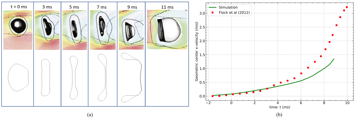
Figure 4: (a) compares Droplet deformation with time for Flock et al. (2012) (top) and analogous Basilisk Simulation (bottom). (b) compares geometric center based x-velocity for Bag breakup case from Flock et al. (2012) to corresponding Basilisk simulations.

It should also be noted that the droplet velocities provided in Flock et al. (2012) are calculated by central difference of the geometric centers of the shadow of the droplet, i.e. outer contour of the droplet as seen from the side, with respect to time. Since the bag in a bag breakup contains a very small fraction of the total droplet volume, a geometric center does not match with volume averaged center of the droplet fluid once the bag has sufficiently inflated. Hence, we obtain geometric centers based droplet velocity from the simulation and use it for comparison.

The comparison between droplet deformation morphology and geometric center x-velocity for experiment and simulation is plotted in figure 4. (a) compares experimental droplet morphology to the corresponding axisymmetric Basilisk simulation. It is observed that the deformation characteristics until time $t=7$ ms is captured very well by the simulations. This includes the shape of pancake and the magnitude of deformation. This is also corroborated by the velocity plot shown in (b), where x-velocity for the experiments and the simulations match very well until approximately $t=6$ ms. Once the droplet deformation reaches the bag inflation stage, the axisymmetric simulations and the experiments start to diverge. Although the general breakup morphology (i.e. bag breakup) is replicated by the simulations, the exact size of the bag and corresponding toroidal rim is not. Since, the droplet shows increasing centroid acceleration as its frontal area increases, a smaller bag size results in smaller accelerations in the simulation.

This divergence of the simulations from experimental results (especially in later stages when the droplet is in bag inflation stage) can be attributed to the differences between the idealized simulation setup and the experiment (as noted previously in detail), i.e. the presence of acceleration due to gravity in the experimental setup and the differences in initial conditions (deformation and velocity) of the droplet. The experiments are inherently not axisymmetric and can only be approximately replicated by an axisymmetric simulation, given the timescales involved in the breakup process are small enough to not allow gravity to have a large effect. Furthermore, the bag rupture process has been canonically attributed to instabilities (Lozano et al., 1998; Bremond & Villermaux, 2005; Villermaux, 2007; Zhao et al., 2011), which cannot be an axisymmetric process. However to fulfill the objectives of this work, accurate information about the exact size of the bag, drop size distribution, or the bag rupture location are not essential. Accurate information about the initial deformation morphology of the droplet, i.e. the pancake shape, and its corresponding general breakup morphology i.e. bag, bag-plume, sheet-thinning, etc. is sufficient to do a broad categorical analysis on the effect of $\mathit{Oh}_{o}$, $\mathit{Oh}_{d}$ and $\rho$ on these features. This information can be reliably obtained through axisymmetric simulations.

2.3.3 Comparison to 3D simulations

To further justify the use of axisymmetric simulations for this work, Basilisk is used to perform both 3D and axisymmetric simulations for multiple cases of low density ratio values. Simulations have been limited to low density ratio values since a high density ratio 3D simulation is computationally unfeasible given the accessible computational resources. Furthermore, as stated by Jain et al. (2019), “For the drops with high $\rho$, flow around the drop has relatively low effect on the drop deformation, morphology and the breakup.” We also choose low Outside Ohnesorge number values (high initial Reynolds number) to ensure that the ambient flow is in turbulent regime. This makes the ambient flow non-axisymmetric since the formation of turbulent vortices is a purely 3D phenomenon, making such flow in theory difficult to perfectly reproduce with only axisymmetric simulations. Such cases are expected to best highlight all the relevant differences (if any) between axisymmetric and full 3D simulations.

Comparison of the variation of fluid interface with time between 3D and axisymmetric simulations for one such case with $\{\rho,\mathit{Oh}_{o},\mathit{Oh}_{d},\mathit{We}_{0}\}=\{50,0.001,0.1,17\}$ is illustrated in figure 5. Under the action of a uniform ambient inflow, the droplet deforms and its deformation with time is shown as a series of VoF plots from left to right. It is observed that the various stages of droplet deformation, from a forward facing pancake (col. 2), to a forward facing bag (col. 3), to its flipping to a backward bag (col. 3-4), is accurately captured by axisymmetric simulations.

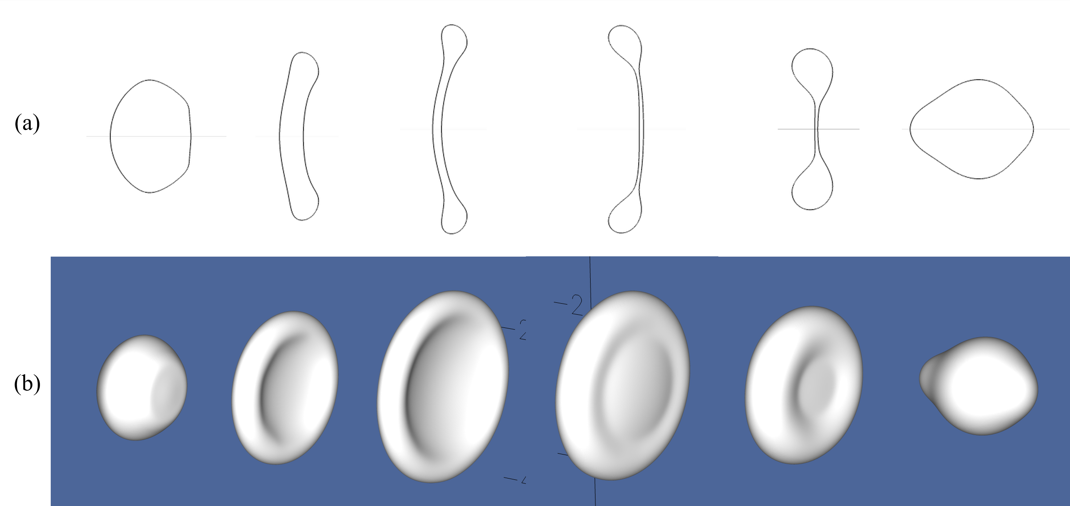
Figure 5: Images in (a) and (b) compare development of the fluid interface with time for axisymmetric and 3D simulations respectively for a case with $\rho=50,\mathit{Oh}_{o}=0.001,\mathit{Oh}_{d}=0.1,\mathit{We}_{0}=17$. The inflow is from left to right, and the corresponding droplet deformation is arranged in the same direction.

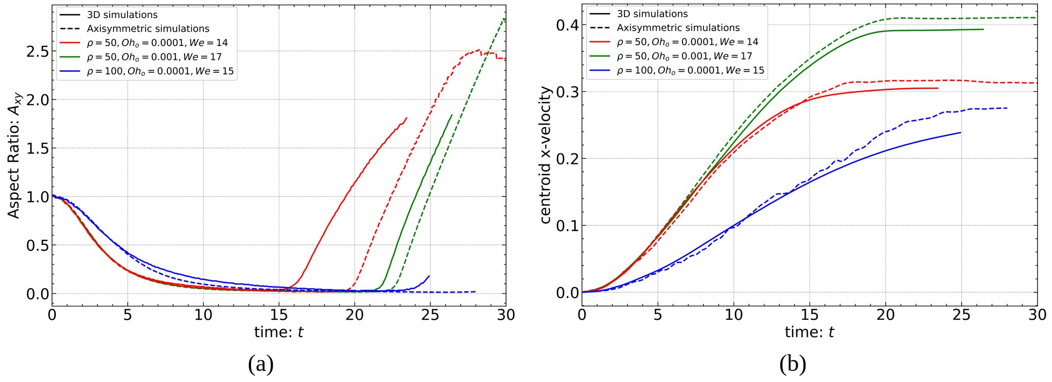
Figure 6: All cases have $\mathit{Oh}_{d}=0.1$ and other non-dimensional parameters as listed in the plots. (a) shows the variation of Droplet Aspect Ratio with time, (b) shows the variation of centroid x-velocity with time, for axisymmetric and 3D simulations.

Figure 6 shows plots for centroid x-velocity and aspect ratio for the three different cases. Both 3D and axisymmetric cases show extremely similar aspect ratios and x-velocities for the majority of the process. Differences between the two simulations start to appear only when the droplets have reached their lowest Aspect ratios and started oscillating back to the equilibrium spherical shape from a flattened pancake position, represented by the increasing $A_{xy}$ (figure 6(a)). This variation in $A_{xy}$ for these small time periods, which is equivalent to differences in corresponding frontal areas, results in small centroid x-velocity differences between axisymmetric and 3D simulations, as can be observed from figure 6(b).

This difference in velocity however is inconsequential in regards to the broader deformation characteristics of a droplet, i.e. the pancake shape and the general breakup morphology. Furthermore, once the droplet has reached its maximum deformation state and has not broken up, its primary deformation process (driven by impulsive acceleration) is complete and the droplet starts the second half of its primary oscillation period. Beyond this stage, the droplet would continue to lose energy to viscous dissipation and hence should never reach deformation levels attained previously. Hence for the purposes of this work, axisymmetric simulations can be considered adequate since our focus is on this primary deformation during the initial half oscillation time period. As discussed in the previous section, the final breakup of a droplet almost always is a sheet breakup which is driven by non-axisymmetric surface instabilities (e.g. Rayleigh-Plateau Instability for rupture of bag), making accurate estimation of statistics such as drop size distribution, the bag size, breakup time, instantaneous velocity during the time of breakup, etc. not achievable through axisymmetric simulations. However for the current work, these statistics are not of interest.

2.4 Parameter space explored

Parameters	Values	Computational cells
$\rho$	$10,50,100,500,1000$	Min: $1.75\times 10^{5}$ Max: $4\times 10^{6}$
$\mathit{Oh}_{o}$	$0.1,0.01,0.001,0.0001$
$\mathit{Oh}_{d}$	$0.1,0.01,0.001$

Table 2: All values of $\rho$, $\mathit{Oh}_{o}$, and $\mathit{Oh}_{d}$ which form the part of the parametric space to be explored through simulations are listed in this table. In total, 60 sets of $\{\rho,\mathit{Oh}_{o},\mathit{Oh}_{d}\}$ are considered, each one is simulated for multiple $\mathit{We}_{0}$ values to obtain its $\mathit{We}_{cr}$. The minimum and maximum number of cells in the computational domain associated with all the simulations is listed in the third column.

The goal of this work is to explore the effect of all the three discussed non-dimensional parameters, i.e. $\rho$, $\mathit{Oh}_{o}$, and $\mathit{Oh}_{d}$ on drop deformation and breakup morphology. Table 2 lists the parameter space explored through simulations in this work. In total, 60 sets of $\{\rho,\mathit{Oh}_{o},\mathit{Oh}_{d}\}$ are represented in this parameter space. Each set is simulated for different $\mathit{We}_{0}$ values to discover its critical Weber number $\mathit{We}_{cr}$ and critical breakup morphology. This is done by simulating each $\{\rho,\mathit{Oh}_{o},\mathit{Oh}_{d}\}$ set with multiple $\mathit{We}_{0}$ values so as to obtain the lowest possible $\mathit{We}_{0}$ value corresponding to which a non-vibrational breakup is observed, i.e. $\mathit{We}_{cr}$.

$Re_{0}\propto 1/\mathit{Oh}_{o}$ and hence for a range of $Re_{0}$ in the order of $(10,10^{4})$, $\mathit{Oh}_{o}$ has a range of $(0.0001,0.1)$. Any higher $\mathit{Re}_{0}$ becomes computationally costly due to significant turbulent vortices in the domain leading to a requirement for higher mesh resolution or even 3D simulations and can also require consideration of compressibility of the flow. Hence, this justifies the specified parameter space decided for $\mathit{Oh}_{o}$.

The impact of $\mathit{Oh}_{d}$ on $\mathit{We}_{cr}$ has been studied for the $\rho$ and $\mathit{Oh}_{o}$ values within the experimentally feasible space. However, the its on both $\mathit{We}_{cr}$ and the corresponding breakup morphology for cases with low $\rho$ or very low or high $\mathit{Re}_{0}$ values has not been explored. In fact, $\mathit{We}_{cr}$ is generally assumed to be constant with respect to $\mathit{Oh}_{d}<0.1$ for all cases in many works. The goal of this work is to explore the validity of these observations for varying $\rho$ and $\mathit{Oh}_{o}$, and hence we chose $\mathit{Oh}_{d}$ to be within $(0.1,0.001)$.

$\rho$ values are varied from $10$ to $1000$ to cover the whole space of low and high density ratio systems.

3 Results

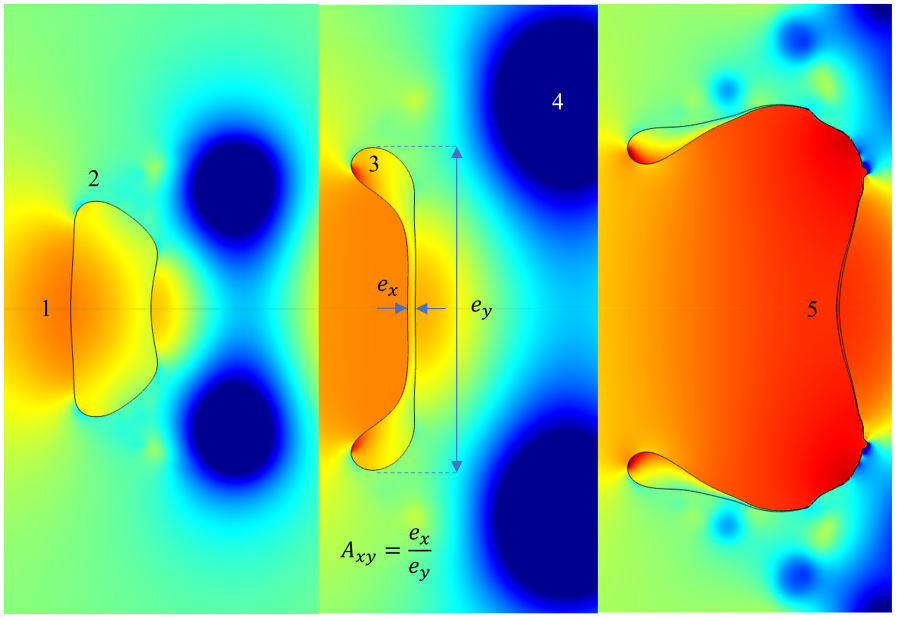
Figure 7: The figure shows the points of interest in a deforming droplet. 1. Upstream pole / Center / Core of the droplet; 2. The periphery of the droplet; 3. The rim of the droplet, which in general has a higher local inertia compared to its center; 4. Downstream low pressure circulation zone, which can affect the motion of its rim if it is attached to the droplet surface (unlike in the figure); 5. The inflated bag, which inflates because of its low inertia and hence higher accelerations.

An example of droplet deformation that starts with the formation of a flat pancake and ultimately breaks up with a backward bag morphology is shown in figure 7. The figure specifies (as numbered markers) some of the important locations and features during droplet deformation. Using this figure as a reference, we define the following factors essential in understanding a droplet’s deformation:

1. The variation of local inertia across the droplet, which determines the local accelerations of each of its parts, e.g. the difference in local inertia between the droplet’s center (1) and rim (3).

2. The pressure difference between its poles (1) and its periphery (2), henceforth denoted by ${\Delta P}_{drive}$. ${\Delta P}_{drive}$ is directly proportional to the stagnation pressures observed at the droplet’s upstream pole.

3. The surface stresses or viscous forces experienced by the droplet’s surface, specially its upstream facing surface. This is a function of the instantaneous Reynolds number $\mathit{Re}$ around the droplet. Since $\mathit{Re}_{0}$ for most situations dictates the order of magnitude of $\mathit{Re}$, $\mathit{Re}$ can be approximated to be equal to $\mathit{Re}_{0}$ if small differences in $\mathit{Re}$ due to centroid accelerations and droplet deformation are not important considerations.

4. The Droplet Ohnesorge number $\mathit{Oh}_{d}$, which can be defined as the ratio of capillary timescale to viscous timescales (equations 12, 13 and 14). It dictates the distribution of the total energy supplied by the ambient flow to the droplet between surface energy change and the fluid momentum developed within the droplet.

From the start of the deformation process until the formation of a proper rim at $t^{*}\approx 1$, a droplet does not have any appreciable variations in local inertia in its lateral dimension. Hence, local inertia differences do not play any role in determining its initial deformation, and is only determined by the competition between pressure and shear forces. Its centroid acceleration, and hence centroid velocity is inversely proportional to its total inertia, which directly affects the instantaneous Reynolds number of the ambient flow past the droplet. The relative velocity of the droplet with respect to the ambient medium dictates the stagnation pressures at its upstream pole and hence its ${\Delta P}_{drive}$. $\mathit{Re}$, on the other hand, dictates the shear stresses acting on its upstream surface. The shape of the pancake then depends on the comparative strengths of this pressure difference and shear forces.

Once a droplet develops local inertia variations across its lateral dimension as it deforms past the pancake stage, any further deformation will be strongly affected by corresponding variations in local accelerations. For the same external forces, the larger inertia parts of the droplet would should much lower accelerations and hence lag behind its low inertia parts.

$\mathit{Re}$ of the ambient flow past the droplet dictates the strength, timescales, lengthscales and location of the downstream vortices (Forouzi Feshalami et al., 2022). It is essential to consider the interaction of these vortices with the droplet’s rim for different $\mathit{Re}$ values to correctly understand its ultimate fate. The sensitivity of the rim to these flow features is almost solely decided by its inertia relative to the ambient fluid, i.e., $\rho$. A large density ratio droplet is expected to show very little sensitivity to downstream vortices, and vice versa.

If we consider the specific droplet case shown in figure 7, the ratio of spatial extent of the droplet along its axisymmetric axis to its spatial extent in y-axis provides the droplet’s Aspect Ratio $A_{xy}$. This parameter will be used in the following sections to quantify the deformation shown by the droplets under specific rheological and flow conditions. In the first image from the left, we observe a flat pancake, which occurs when ${\Delta P}_{drive}$ predominantly drives the internal flow in the droplet (over shear stresses). We also observe a clear toroidal rim (image 2) which has a large local inertia, and hence is expected to lag the lower inertia center of the droplet. Due to its large inertia, the droplet’s rim remains unaffected by the low pressure zone created by the downstream vortex, which sheds a sufficient distance away from the rim and is not attached to the droplet. Ultimately, the droplet deforms into a backward bag breakup morphology as the center inflates into a bag under the action of pressure forces at its stagnation point.

3.1 Density Ratio

This section illustrates the role density ratio plays in dictating droplet deformation and breakup morphology. In figure 8(a), variation of droplet centroid velocity and Aspect Ratio ($A_{xy}$) (defined in figure 7) with time for density ratios from $10$ to $1000$ is plotted. The centroid velocity plot show the direct effect of total inertia of the droplet on its centroid acceleration. The lowest $\rho$ droplets experience the highest centroid accelerations and hence tend to achieve free-stream velocity the fastest. This leads to lower stagnation pressures at the upstream poles of low $\rho$ droplets, and also results in lower $\mathit{Re}$ values. This can also be interpreted as the sensitivity of the droplet to external forces, i.e. a droplet with a large $\rho$ will show smaller local accelerations due to external forces compared to low $\rho$ droplets under the same forces in the same time interval. Hence, a droplet’s response to downstream vortices would directly depend on its $\rho$.

The temporal development of aspect ratio for cases with different $\rho$ values is also shown in figure 8(a). Up until the completion of pancake formation at $t^{*}\approx 1$, all the droplets show a similar decrease in their $A_{\mathit{xy}}$ values with time. This stage belonging in $0<t^{*}<1$ corresponds to the the longitudinal flattening of the droplet from a sphere to a pancake. At $t^{*}\approx 1$, the droplet achieves its lowest aspect ratio as a pancake. Any further deformation past pancake stage leads to formation of a clear prominent rim, which marks the end of this stage.

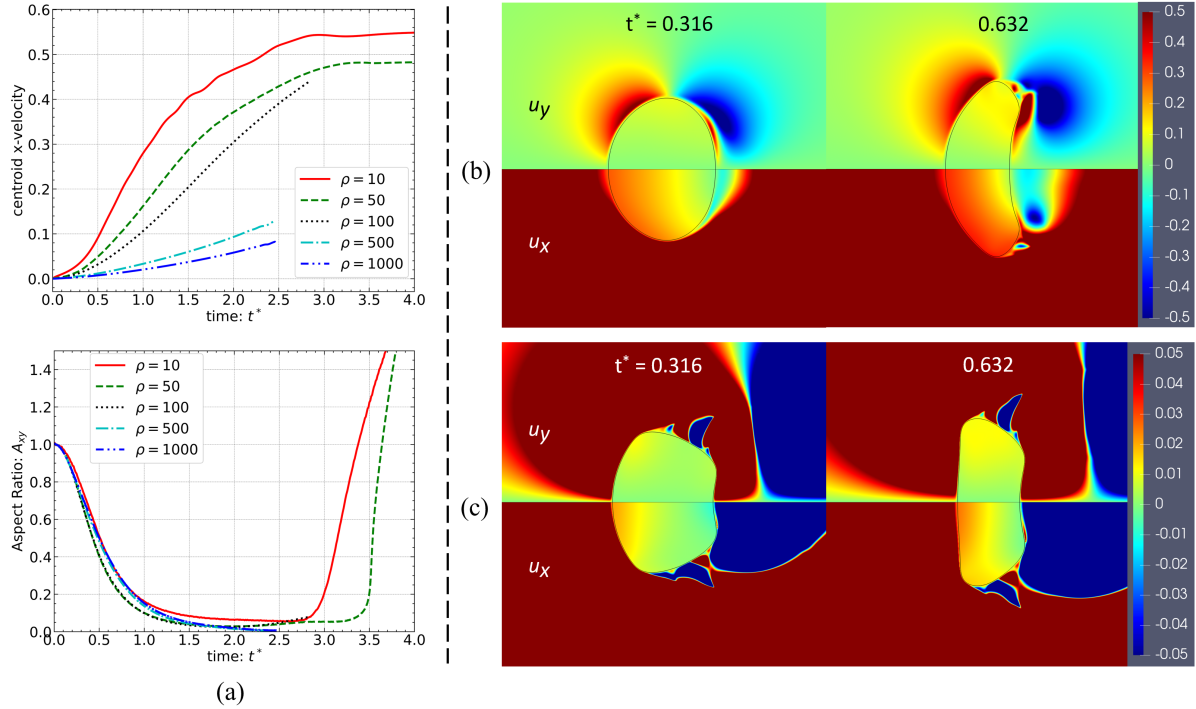
Figure 8: (a) shows the temporal variation of centroid x-velocity and Aspect Ratio of droplets with different $\rho$ values. Internal velocity fields are plotted for (b) $\rho=10$ and (c) $\rho=1000$. The upper half shows y-velocities, whereas the lower half of each plot shows x-velocities. All droplets referred here have $\mathit{Oh}_{o}=0.001$, $\mathit{Oh}_{d}=0.1$, $\mathit{We}_{0}=20$.

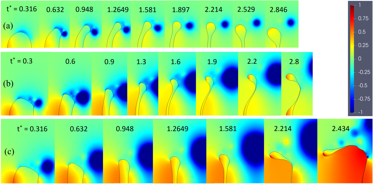
Figure 9: Pressure field plots for droplets with three different density ratios are plotted (a) $\rho=10$ (b) $\rho=100$ (c) $\rho=1000$ for a low $\mathit{Oh}_{o}$ system. All droplets referred here have the following common parameters: $\mathit{Oh}_{o}=0.001$, $\mathit{Oh}_{d}=0.1$, $\mathit{We}_{0}=20$.

Let us start with the effect of density ratio on low ambient Ohnesorge number ($\mathit{Oh}_{o}$) droplet-ambient systems. The plots relevant to these cases are presented in figure 8(b), (c) and 9. The common $\mathit{Oh}_{o}$ for the corresponding cases is $\mathit{Oh}_{o}=0.001$ which corresponds to a $\mathit{Re}_{0}\approx 4472$. This high $\mathit{Re}_{0}$ results in low shear stresses acting on the upstream surface of the droplet, compared to a high $\mathit{Oh}_{o}$ case (such as $\mathit{Oh}_{o}=0.1$ in figure 10).

Up until the formation of a clear toroidal rim at $t\approx 1$, local inertia differences across the droplet are small, and hence do not play a role in deciding local accelerations under the same external forces. Hence, during the pancake formation stage, its deformation is dependent only on the balance between the shear and pressure forces applied on it by the ambient medium.

A low $\rho$ droplet has lower relative velocities with the free-stream compared to a high $\rho$ droplet, which leads to low pressure difference between its upstream pole and its periphery (${\Delta P}_{drive}$). This is illustrated through the pressure field plots for $\rho=10$ case in figure 9(a) for which the lowest stagnation pressures are observed. This low ${\Delta P}_{drive}$ is what enables even the low shear stresses applied by the low $\mathit{Oh}_{o}$ (i.e., high $\mathit{Re}_{0}$) ambient flow to be the dominant factor. Hence, we expect its initial deformation and internal flow to be predominantly driven by shear stresses acting on its upstream surface. This is verified through the internal flow plots corresponding to figure 9(a) shown in figure 8(b). The internal flow is highest at its upstream surface and shows a decrease to nearly zero at its downstream pole (see $u_{x}$), in a direction normal to its upstream surface. This flow profile directly points to its internal flow characteristics to being dictated by the shear stresses. We also observe that the internal velocities near the droplet’s periphery are the largest, which points to its periphery experiencing the largest velocity gradients, and hence the largest shear stresses. This together with the lack of local inertia differences across the droplet’s lateral dimension (before $t^{*}\approx 1$) results in larger local acceleration at its periphery compared to its center, leading to a forward facing pancake. Additionally, due to its lower relative deficit with the ambient medium, its $\mathit{Re}$ is lower than that of a high $\rho$ droplet and hence results in a weak downstream circulation zone. Given its low inertia, the droplet’s rim still shows a small sensitivity to the weak induced drag applied by this downstream vortex, contributing to the forward pancake morphology. The vortex hence does not fully detach from the droplet’s rim and sheds nearer to its periphery during its pancake formation stage.

This dominance of shear stresses over ${\Delta P}_{drive}$ is not as clear for an intermediate $\rho$ droplet such as the one shown in figure 9(b), for which the stagnation pressures observed is higher than that in (a). This increased ${\Delta P}_{drive}$ is large enough to match shear stresses’ contribution to the internal flow in the droplet, leading to a pancake which is somewhere between a flat and a forward facing shape.

For the large $\rho$ droplet shown in figure 9(c), the stagnation pressures are even higher, which makes ${\Delta P}_{drive}$ the dominant factor over the shear stresses in deciding its internal flow. This is evident from its internal flow as shown in figure 8(c). The highest x-velocities are seen at its upstream pole, and not at its periphery as was seen for the $\rho=10$ case (figure 8(b)).

Once the droplet starts deforming beyond pancake shape (at $t^{*}\approx 1$), the formation and growth of a prominent rim is observed for all three cases shown in figure 9. Once a major fraction of the droplet fluid has been transferred to its rim, local inertia differences between its center and its periphery begin to affect the local accelerations of different parts of the droplet. Furthermore, as the droplet deforms further towards a bag morphology, the radius of its frontal area also increases. In some cases (such as for $\rho=1000$), this radial increase can offset the reduction in its velocity deficit with the ambient, increasing its $\mathit{Re}$, ultimately leading to the low pressure circulation zone downstream of the droplet to grow stronger. Additionally, given the $\rho$ (i.e., its inertia relative to the ambient medium) of the droplet-ambient system is not very large, the droplet’s rim may appreciably interact with this downstream low pressure zone, experiencing an induced drag, and possibly even forming a forward bag shape.

For a low $\rho$ case such as figure 9(a), its downstream vortex shows very little growth, owing to its substantially large centroid velocities, and comparatively small radial growth. By $t^{*}=1.581$, the little induced drag experienced by the droplet’s rim is overcome by the local inertia differences between its center and periphery. Its rim starts to slow down relative its center, and begins flipping from a forward to a backward bag morphology. By $t^{*}=1.897$, its downstream vortex has fully developed and detached from its periphery, and hence plays no further role in determining its deformation. Due to its low relative velocities with the ambient medium, the total aerodynamic forcing driving its deformation is small. The droplet hence reaches a bag morphology at $t^{*}=2.214$ but does not sufficiently deform to cause a breakup.

For a high $\rho$ case such as figure 9(c), owing to its high relative velocities with respect to the free-stream, coupled with the large growth in its radial dimension, its downstream circulation zone is much stronger. However, its high inertia leads to the droplet’s rim showing very little sensitivity to the induced drag applied by the downstream vortex. This allows the droplet to detach from its downstream vortex even as early as $t^{*}=0.632$, and hence experiences negligible local induced drag at its rim past $t^{*}=0.632$. This along with the already dominant ${\Delta P}_{drive}$ leads to only lateral growth of the pancake (flattening) from $t^{*}=0.948$ to $t^{*}=1.581$. Once the local inertia differences between its center and periphery have grown to a substantial degree, as seen at $t^{*}=1.581$, its rim starts to decelerate relative to its center due to its lower local accelerations, and hence forms a backward bag. Figure 9(c) shows this behavior from $t^{*}=1.581$ to $t^{*}=2.434$.

For the intermediate $\rho$ case shown in figure 9(b), neither the pressure forces nor the local inertia differences completely dominate the droplet’s deformation beyond the formation of pancake, which allows this droplet to show a different behavior compared to the other two cases. Droplet in (b) has a larger inertia compared to (a), which leads to a stronger downstream circulation zone (owing to the larger $\mathit{Re}$). In addition, even the formation of a clear rim at $t^{*}=0.9$ does not generate enough local acceleration differences to allow its periphery to detach from the developing circulation zone. Its rim thus experiences considerable induced drag, resulting in some displacement downstream of its rim relative to its core from $t^{*}=0.9$ to $t^{*}=1.6$. This results in the droplet showing a larger rate of lateral stretching compared to the rate of evacuation of its core (which is dependent on ${\Delta P}_{drive}$). The droplet starts its bag inflation process, even while its central core is not fully evacuated and contains some remnant droplet fluid (see $t^{*}=1.9$). This remnant fluid core is also called a plume. A similar explanation for the formation of plume is provided in Jackiw & Ashgriz (2021), where a faster inflation of bag (due to higher $\mathit{We}_{0}$ in the paper) compared to the movement of droplet fluid from its center to its rim leads to the presence of an undeformed core at the droplet’s center. Volume of this undeformed core dictates which specific breakup is observed: bag-plume, multibag or sheet thinning. While the droplet is being laterally stretched, its rim has gained enough inertia by $t^{*}=1.9$ to show lower local accelerations. This is when the droplet’s rim and core start to lag behind the toroidal bag connecting the two, forming a backward-plume bag. This deformation process is also shown in Marcotte & Zaleski (2019) (in figure 4) for a low $\mathit{Oh}_{o}$ case where a variation in $\rho$ from $10$ to $2000$ is accompanied with a shift in pancake and breakup morphology exactly as has been observed here.

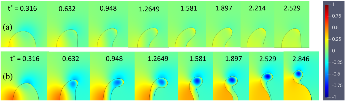
Figure 10: Pressure field plots are plotted for two different $\rho$ values for a high $\mathit{Oh}_{o}$ ambient flow. (a)$\rho=10$ (b)$\rho=1000$. All droplets shown here have the following common parameters: $\mathit{Oh}_{o}=0.1$, $\mathit{Oh}_{d}=0.1$, $\mathit{We}_{0}=20$.

Let us now shift our attention to the effect of $\rho$ on high $\mathit{Oh}_{o}$ cases. Figure 10 shows the variation of pressure field around the droplets with time. For both these cases, $\mathit{Oh}_{o}$ is $0.1$ which corresponds to a $\mathit{Re}_{0}=44.72$. For such low $\mathit{Re}_{0}$, we expect the shear stresses on the its upstream surface to be substantial. Hence, even though we see a substantially higher upstream stagnation pressure and hence a higher ${\Delta P}_{drive}$ for (b) ($\rho=1000$) compared to (a) ($\rho=10$), pressure differences still do not dominate over the shear stresses in deciding its internal flow during pancake formation. As expected, we see a forward pancake at $t^{*}=0.948$ for both cases. Furthermore for both cases, due to the low $\mathit{Re}_{0}$ of the flow, the ambient flow remains completely attached to the droplet’s surface, eliminating the formation of any downstream circulation zones. Hence, the droplet’s rim does not have a source for any additional external forces to counteract its growing inertia, and a backward bag becomes the only possible morphology. (b) shows a backward bag breakup, while (a) shows much smaller deformations and does not breakup. Since, droplet (a) experiences much lower external forces due to experiencing lower relative velocities, its lower deformation is an expected observation.

In conclusion, the morphology of the pancake depends on the competition between the pressure differences between the poles and the periphery of the droplet, and the shear stresses acting on its upstream surface. When ${\Delta P}_{drive}$ is dominant, we see a flat pancake. When shear stresses are dominant, we see a forward facing pancake. As the droplet deforms past a pancake, it forms a bag, which can either be forward or backward, depending on the local inertia of the rim and the ambient Ohnesorge number. While local inertia is dependent on $\rho$ and the rate of evacuation of fluid from droplet’s core, strength and location of downstream vortices depends on $\mathit{Oh}_{o}$ and the instantaneous centroid velocity of the droplet, which again depends on its inertia $\rho$. Finally, the droplet can also form a plume given it experiences a larger rate of stretching compared to its internal flow moving fluid away from its core, which is dependent on ${\Delta P}_{drive}$.

3.2 Ambient Ohnesorge number

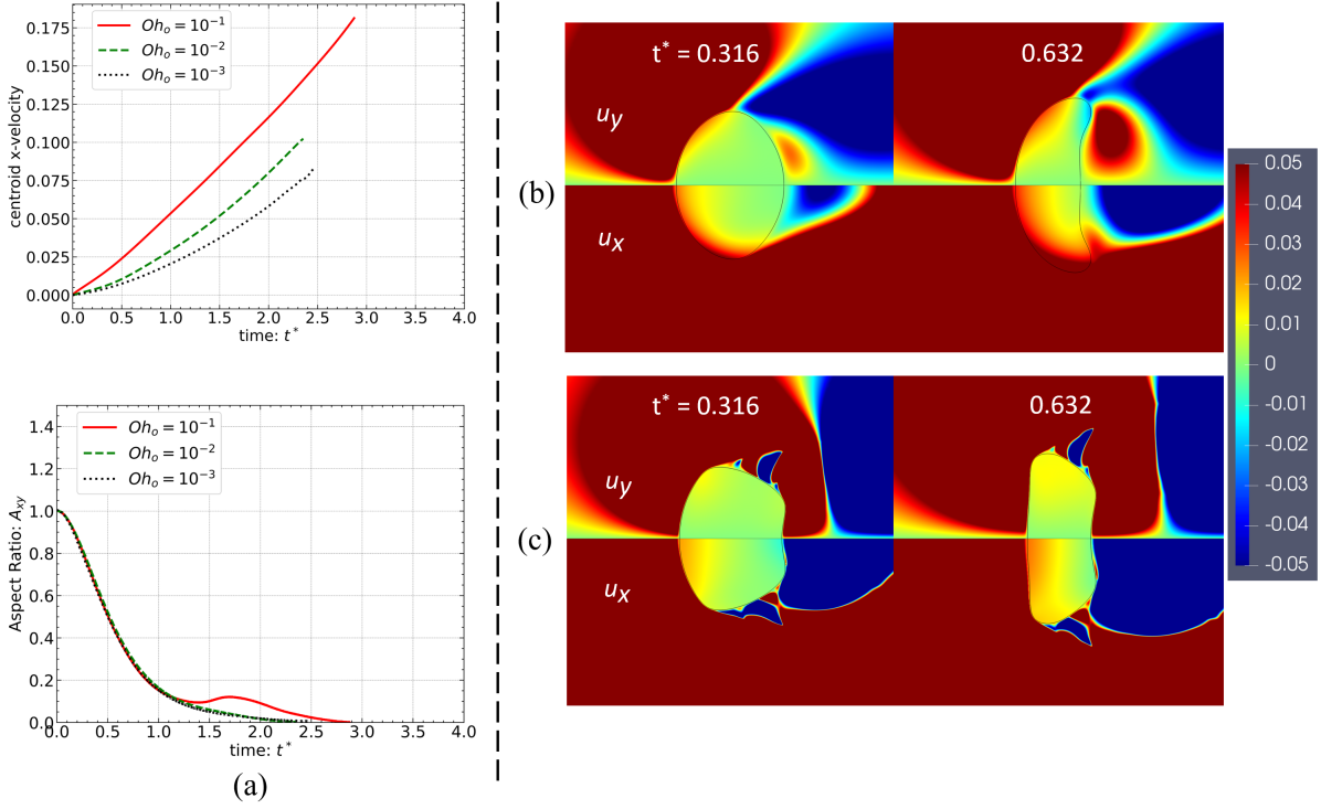
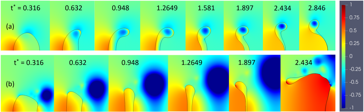
Figure 11: For all plots shown here, $\rho=1000$, $\mathit{Oh}_{d}=0.1$ and $\mathit{We}_{0}=20$. (a) shows the temporal variation of droplet centroid x-velocity and Aspect ratio for different $\mathit{Oh}_{o}$ values. Velocity fields are plotted for (b) $\rho=10$, (c) $\rho=1000$.

Figure 12: Both the droplets shown here have $\rho=1000$, $\mathit{Oh}_{d}=0.1$ and $\mathit{We}_{0}=20$. Pressure fields are shown for droplets with (a)$\mathit{Oh}_{o}=0.1$, and (b)$\mathit{Oh}_{o}=0.001$.

Figure 12(a) plots the effect of $\mathit{Oh}_{o}$ on temporal variation of droplet centroid velocities and aspect ratios. $\mathit{Oh}_{o}$ values range from $0.1$ ($\mathit{Re}_{0}=44.72$) to $0.001$ ($\mathit{Re}_{0}=4472$) for both plots. We observe that the flows with highest $\mathit{Oh}_{o}$ values show the highest droplet centroid velocities. This can be attributed to the higher shear stresses experienced by the droplet in high $\mathit{Oh}_{o}$ flows (which corresponds to high ambient dynamic viscosity), which leads to larger droplet centroid acceleration. A lower velocity deficit with the ambient medium is expected to result in lower stagnation pressures, and hence lower ${\Delta P}_{drive}$ values. As was seen previously in figure 8(a), all the droplets also show very similar temporal development of their aspect ratios.

We start with a description of the effect of $\mathit{Oh}_{o}$ on the deformation of high density ratio droplets. Pressure fields for two different $\mathit{Oh}_{o}$ values for $\rho=1000$ have been plotted in figure 12. All non-dimensional parameters except $\mathit{Oh}_{o}$ are the same for the two cases.

For the droplet in figure 12(a), $\mathit{Oh}_{o}=0.1$, i.e. $\mathit{Re}_{0}$ is very low which corresponds to a large outside viscosity. This in addition to the flow not detaching from the droplet’s surface leads to large viscous stresses on its upstream surface, and consequently larger centroid velocities. The droplet in figure 12(b) on the other hand has a $\mathit{Re}_{0}$ value which is 100 times larger, leading to much smaller shear stresses and consequently smaller centroid velocities. A higher velocity deficit with the ambient results in (a) experiencing smaller stagnation pressures and hence smaller ${\Delta P}_{drive}$ compared to (b).

It should be noted that the effective shear stresses experienced by a droplet more accurately depends on its instantaneous Reynolds number $\mathit{Re}$, which is lower than $\mathit{Re}_{0}$ owing to the non-zero centroid velocities of the droplet. However, this reduction plays a minor role in affecting the shear stresses when compared to the two orders of magnitude increase in $\mathit{Re}_{0}$ between the two cases.

Hence for the droplet in figure 12(a), the shear stresses acting on its upstream surface dictates its initial internal flow and corresponding deformation. This is evident from its internal flow plot shown in figure 12(b), which is highest at its upstream surface and decreases to zero at its downstream pole. The highest internal velocities occur at the periphery of its pancake, which coincides with the location of largest shear stresses applied by the ambient flow. This results in the formation of a forward facing pancake.

For the droplet in figure 12(b) on the other hand, shear stresses are significantly lower and do not dominate the even larger ${\Delta P}_{drive}$ values (compared to (a)), thus resulting in a flat pancake. Its highest internal velocities occur at its upstream pole, and not at its periphery, as seen in figure 12(c).

It is interesting to note the differences in droplet deformation between figure 12(b) and figure 9(a). The low density ratio ($\rho=10$) case shows much smaller pressure differences compared to the high density ratio ($\rho=1000$) case even though the two flows have the same $\mathit{Re}_{0}$. This is due to its low inertia, which allows the droplet to show comparatively higher centroid accelerations, and hence centroid velocities, thus reducing its velocity deficit with respect to the ambient flow. This lower velocity deficit results in lower stagnation pressures and $\mathit{Re}_{0}$ values for the low $\rho$ case compared to the high $\rho$ ($=1000$) case, which in turn leads to larger shear stresses on its upstream surface. This combination of lower ${\Delta P}_{drive}$ and higher shear stresses results in the droplet in figure 9(a) showing a forward pancake.

In a nutshell, the orientation of the pancake (which is a direct result of the competition between ${\Delta P}_{drive}$ and shear stresses) depends on both $\rho$, due to its significant impact on ${\Delta P}_{drive}$, and $\mathit{Oh}_{o}$, due to its significant impact on the $\mathit{Re}$ and hence the shear stresses acting on the droplet.

As the droplets deform further, both cases develop a prominent rim, which creates a substantial difference in local inertia between the rim and the center (prospective bag) of the droplet. For case (a), owing to the extremely low $\mathit{Re}$ of the flow, the flow remains attached with the droplet and hence does not form a downstream vortex. Case (b) does form a downstream circulation zone, but its large local inertia (i.e. $\rho$) allows the vortex to detach early from the droplet. Hence for both cases, the rim does not experience any additional forces that can offset the effect of its higher local inertia at its rim on the corresponding local acceleration, leading to case (a) flipping its orientation from a forward pancake to a backward bag, while (b) forms a backward bag from a flat pancake.

An example illustrating the effect of $\mathit{Oh}_{o}$ on intermediate density ratio ($\rho=100$) droplets is shown in figure 14. The two cases differ only in their values of $\mathit{Oh}_{o}$ with (a) $\mathit{Oh}_{o}=0.001$ and (b) $\mathit{Oh}_{o}=0.0001$. Both cases have relatively high outside Reynolds numbers. However, (b) has its $\mathit{Re}_{0}$ ($\approx 36055$) firmly in the free shear regime (Forouzi Feshalami et al., 2022), leading to much smaller and intense turbulent vortices with smaller vortex timescales downstream of the droplet. This leads to the generation of many small vortices which shed very close to the droplet periphery compared to (a). The lower $\mathit{Re}_{0}$ of case (a) on the other hand shows a distinct solitary circulation zone which, as expected, is larger in size and is detached from the droplet. In addition, owing to their intermediate $\rho$ values, the droplets show centroid accelerations and instantaneous centroid velocities somewhere in between that of high and low $\rho$ cases. The ${\Delta P}_{drive}$ values (dependent on velocity deficit with respect to ambient) observed for both cases are hence of the same magnitude scale as the shear stresses (dependent on $\mathit{Re}$) acting on their upstream surfaces (similar to figure 9(b)) in driving their respective internal flows. Hence, the pancake shape for both (a) and (b) is somewhere between a forward and a flat pancake. The only observable difference between the two cases in their pancake formation stage ($t^{*}<1$) is the more intense surface perturbations seen in (b), which results from the many smaller vortices forming around the droplet, coupled with the low viscous damping provided by both the droplet and the ambient fluid (corresponds to the low $\mathit{Oh}_{d}$ and $\mathit{Oh}_{o}$ values respectively).

Figure 13: Both cases shown here have $\rho=100$, $\mathit{Oh}_{d}=0.001$ and $\mathit{We}_{0}=13$. (a), (c) and (e) plot pressure field, vorticity and y-velocity for droplet with $\mathit{Oh}_{o}=0.001$; whereas (b), (d) and (e) plot the same for droplet with $\mathit{Oh}_{o}=0.0001$.

Figure 14: Both cases shown here have $\rho=50$, $\mathit{Oh}_{d}=0.1$ and $\mathit{We}_{0}=20$. (a) and (c) plot y-velocities and pressure field for droplet with $\mathit{Oh}_{o}=0.01$; whereas (b) and (d) plot y-velocities and pressure field for droplet with $\mathit{Oh}_{o}=0.001$.

Once a clear rim forms for the droplets in figure 14 (at $t^{*}\approx 1.3$), their deformation paths diverge. For the droplet in case (a), its rim is well developed and has a proper toroidal structure leading to significant inertia differences from its center. However, as its $\rho$ value is not very large, its rim shows a not insignificant sensitivity to the induced drag applied by the downstream circulation zone, leading to the slightly forward facing pancake observed at $t^{*}=1.3$ for (a).

The droplet in case (b) has the same intermediate $\rho$ but a larger $\mathit{Re}_{0}$, and hence is subjected to downstream vortices that are generated much closer to its periphery. Its rim strongly interacts with this low pressure zone and is pulled downstream due to the corresponding induced drag (substantially larger compared to (a)).

This interaction with downstream vortices also leads to an increase in the rate of stretching of the droplet from its upstream pole to periphery. This observation is supported by the y-velocity plots for both droplets (a) and (b) as shown in figure 14(e) and (f) respectively. Both plots show substantially larger y-velocities at their periphery compared to their centers. The evacuation rate of fluid from a droplet’s core is directly proportional on its ${\Delta P}_{drive}$, which is quite similar for both cases and not particularly large due to their (equal) intermediate $\rho$ values (i.e., (almost equal) intermediate centroid velocities). Thus, the increased rate of stretching seen in the two droplets is not matched by the mediocre rates of evacuation of their cores, ultimately leading to the formation of a plume in both droplets which creates two high inertia regions at their cores and their periphery. However comparing between the two cases, the higher $\mathit{Re}_{0}$ case (f) shows a larger rate of lateral stretching since it experience stronger induced drag due to having better access to its downstream vortices.

Ultimately, the droplet in figure 14(a) owing to its well-formed high inertia rim, breaks up with a backward bag-plume morphology. The droplet in figure 14(a) on the other hand, due to its faster stretching forms a larger plume, preventing the formation of a clear high inertia rim. Its bag hence never escapes the downstream low pressure zone and ultimately breaks up in a forward bag morphology.

In short, the rate of stretching and size of plume a droplet experiences increases with the increase in proximity and strength of downstream vortices to its rim (due to increase in $\mathit{Re}_{0}$). Hence, this forward bag-like structure is only observed (for low $\mathit{We}_{0}$ simulations) when $\mathit{Oh}_{o}$ values are small (preferably in the shear layer instability regime, i.e. $1000\leq\mathit{Re}_{0}\leq 10^{5}$) and $\rho$ is small. A high density ratio case such as $\rho=1000$ shows forward bag breakup in the current simulations only for $\mathit{Oh}_{o}=0.0001$.

Figure 14 shows another example where decreasing $\mathit{Oh}_{o}$ motivates the formation of a plume. Since $\rho$ for both cases is small, both shear stresses and ${\Delta P}_{drive}$ equally affect the droplet’s internal flow, which leads to a partially forward facing morphology. Hence, the downstream vortex is not completely isolated from its rim. Furthermore, compared to (a), droplet (b) shows a stronger downstream vortex due to its larger $\mathit{Re}_{0}$ as shown in figure 14(e) and (f). Hence, the induced drag on its rim is larger which leads to a higher rate of stretching compared to (a). This is evident from the y-velocity plots for the two cases as shown in figure 14(a) and (b), with (b) showing much larger y-velocities at its rim. We hence see a plume for the lower $\mathit{Oh}_{o}$ case which leads to the formation of an annular bag between the center and the periphery, i.e. backward bag-plume morphology. The larger $\mathit{Oh}_{o}$ case shows a simple backward bag breakup.

In conclusion, a decrease in Outside Ohnesorge number motivates formation of both forward bag as well as plume. Whether the final breakup morphology is a forward bag (with no clear high local inertia region in the deformed droplet) or a backward bag-plume breakup (with its rim and core both having large local inertia) depends on both the droplet’s density ratio and if the outside Reynolds number is in the shear layer instability regime.

3.3 Drop Ohnesorge Number

We start with an analysis of cases with high $\rho$ and low $\mathit{Oh}_{o}$. Droplets in such droplet-ambient systems experience low centroid accelerations, and hence low centroid velocities. Thus, velocity deficits with the ambient medium remain high, leading to large stagnation pressures and $\mathit{Re}$ values. Shear stresses acting on the upstream surface of these droplets are hence low owing to the high $\mathit{Re}_{0}$. This results in ${\Delta P}_{drive}$ dominating the process of pancake formation, and dictates the flow inside the droplet resulting in a flat pancake. Furthermore, given all other parameters are the same between the two cases, a larger $\mathit{Oh}_{d}$ is equivalent to a larger droplet viscosity $\mu_{d}$. It is hence expected to see lower internal flow velocities and internal circulations for the high $\mathit{Oh}_{d}$ cases. Higher $\mu_{d}$ also corresponds with an exponential decrease in the incidence of surface instabilities (Fuster et al., 2009). For the same forcing, a capillary wave is more stable given higher surface tension and droplet viscosity. While surface tension plays a major role in deciding the wavelength of the highest amplitude capillary wave, an increase in $\mu_{d}$ increases the length and timescales for which a capillary peak generated by an instability remains stable. As a droplet accelerates, the forcing on the droplet reduces over time and hence an unstable peak might survive due to not getting sufficient time to show breakup, given $\mu_{d}$ has sufficiently increased its survival lengthscales and timescales (Goodridge et al., 1997).

Figure 16 illustrates the pressure fields for two such cases with only $\mathit{Oh}_{d}$ as the varying parameter and $\rho=1000,\mathit{Oh}_{o}=0.001$. Both cases show very similar (high) stagnation pressures and an $\mathit{Re}_{0}$ of $4472$ results in an well-defined downstream vortex, which is detached from their periphery. This in conjunction with the large inertia of these droplets elicits negligible forward motion of their periphery with respect to their cores. As expected at $t^{*}\approx 1$, both cases show a flat pancake and start of rim formation. However, for case (b), we observe a high pressure zone at the upstream pole, which hints to the start of a plume. The internal flow of the droplet shown in figure 16(b) hints at its cause. An instability appears at its upstream pole which motivates a flow from the periphery to the upstream pole of the droplet hugging its upstream surface. A larger $\mu_{d}$ tends to dampen out possible instabilities discouraging the appearance of such plumes. Given (b) has a droplet viscosity 100 times smaller compared to (a), the development of a prominent capillary instability and corresponding pancake shape is reasonable. Furthermore, the instability arises at the upstream pole, which is a stagnation point and sees the highest accelerations of any location on the droplet. This matches with the definition of Rayleigh-Taylor instabilities, and might be the primary mechanism behind the development of a plume of this kind. According to Villermaux (2007) Jalaal & Mehravaran (2014), an increase in density discontinuity motivates the formation of RT instability. This behavior is observed in current simulations as well, as only the cases with $\rho=500$ or $1000$ and for the lowest $\mathit{Oh}_{d}$ values form an unstable plume.

In both cases, as the droplets deform further and their rims gain a larger share of their total mass, differences in local inertia across the droplets start getting substantial enough for local accelerations to be different. Their rims (which have higher inertia) start to lag behind relative to their centers. However for case (b), the plume has grown further and the droplet now has two high local inertia regions: its core due to the presence of the plume, and its rim. The part of the droplet connecting its core and rim (an annulus) has lower local inertia compared to both these regions, and hence accelerates relative to both leading to the growth of a bag between the plume and the rim. Ultimately, this annular bag breaks up and leads to a backward bag-plume breakup as seen in (b).

Figure 15: All droplets in these plots have $\rho=1000$, $\mathit{Oh}_{o}=0.001$, $\mathit{We}_{0}=20$. These Plots show internal flows for two different $\mathit{Oh}_{d}$ values: (a)$\mathit{Oh}_{d}=0.1$, and (b)$\mathit{Oh}_{d}=0.001$. (c) is a zoomed in view of $t^{*}=1.2649$ for (b)

Figure 16: All droplets in these plots have $\rho=1000$, $\mathit{Oh}_{o}=0.001$, $\mathit{We}_{0}=20$. These plots show the pressure fields around droplets of different $\mathit{Oh}_{d}$ values. (a)$\mathit{Oh}_{d}=0.1$ (b)$\mathit{Oh}_{d}=0.001$.

For the droplet in figure 16(b), it should be noted that a reduction in $\mathit{We}_{0}$ (with all other parameters the same) still leads to the generation of an instability on its upstream pole leading to a plume, albeit of a smaller size. At $\mathit{We}_{0}=16$, the pancake with plume does not deform enough to show a bag-plume breakup. $\mathit{We}_{0}$ has to be reduced even further for plume to stop appearing. Hence, a reduction in $\mathit{We}_{0}$ cannot not lead to a simple bag breakup for the specific non-dimensional parameter set. This makes a backward bag-plume breakup the critical breakup morphology for this case: a feature of the rheology of the system ($\rho$, $\mathit{Oh}_{d}$ and $\mathit{Oh}_{o}$), and not just a function of $\mathit{We}_{0}$.

In contrast to the plume seen in figure 16(b) which emerges from an instability at upstream pole at $t^{*}\approx 1$, a decrease in $\mathit{Oh}_{d}$ can also lead to a plume similar to that in figure 14(b). One such example is shown in figure 18. In the context of droplets, $\mathit{Oh}_{d}$ can be interpreted as the ratio of capillary timescale ($T_{\sigma}$) (equation 12), defined as the time required for a capillary wave of wavelength D to travel a lengthscale D; to the viscous timescale ($T_{\mu}$) (equation 13), defined as the time it takes for momentum to diffuse across the droplet (Popinet, 2009).

$$T_{\sigma}=\sqrt{\dfrac{\rho_{d}D^{3}}{\sigma}}$$ (12)

$$T_{\mu}=\dfrac{\rho_{d}D^{2}}{\mu_{d}}$$ (13)

$$\mathit{Oh}_{d}=\dfrac{T_{\sigma}}{T_{\mu}}=\dfrac{\mu_{d}}{\sqrt{\sigma\rho_{d}D}}$$ (14)

A smaller $\mathit{Oh}_{d}$ can be thought of as a small $T_{\sigma}$ compared to $T_{\mu}$, i.e. information about interface deformation travels much faster compared to the corresponding momentum transferred (internal flow velocities gained) to the droplet fluid across its dimension. Hence, the downstream vortices could apply some induced drag on the droplet’s rim, causing it to show some local acceleration and hence deformation, but not generate similar movement of the total droplet fluid. This is evident from the y-velocity plots shown in figure 18, where the lower $\mathit{Oh}_{d}$ case (b) shows larger y-velocities at its rim, i.e. a larger rate of stretching compared to the higher $\mathit{Oh}_{d}$ case (a). Both cases have intermediate density ratio values ($\rho=100$) which allows their periphery to be appreciably affected by downstream low pressure zones, and experience some lateral stretching. In addition, the rate of evacuation of fluid from the core of a droplet is strongly dependent on ${\Delta P}_{drive}$ which is very similar for the two cases. Hence, case (b) which shows larger lateral stretching due to its lower viscosity forms a plume. It is essential to note that the droplet in this case only shows a plume once it has started to form a bag. The initial pancake is still flat. Plume in figure 16(b) however develops very early in the deformation process, right at the instant of formation of the pancake. Hence, the two types of plumes are fundamentally different in their formation mechanisms.

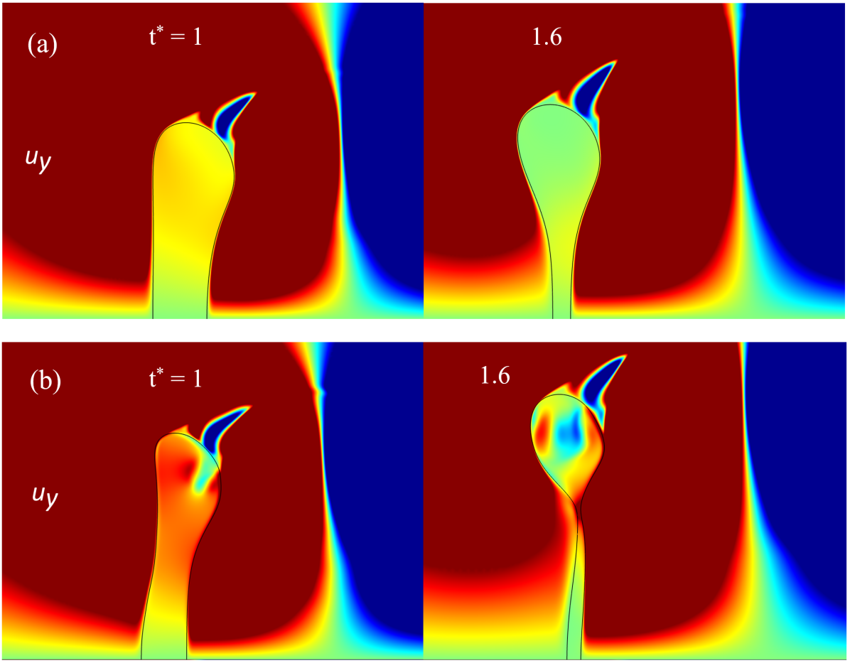
Figure 17: Both cases have $\rho=100$, $\mathit{Oh}_{o}=0.001$, $\mathit{We}_{0}=13$. These plots show y-velocities for two different $\mathit{Oh}_{d}$ values: (a)$\mathit{Oh}_{d}=0.1$, and (b)$\mathit{Oh}_{d}=0.001$.

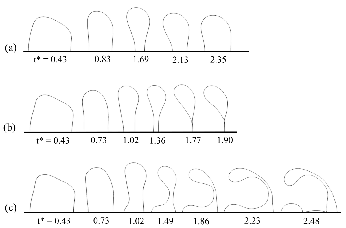
Figure 18: These plots show the fluid interface for three cases with $\rho=1000$, $\mathit{Oh}_{o}=0.001$, $\mathit{We}_{0}=15$, and (a) $\mathit{Oh}_{d}=0.1$ (b) $\mathit{Oh}_{d}=0.01$ (c) $\mathit{Oh}_{d}=0.001$.

According to most of the current literature, if $\mathit{Oh}_{d}\leq 0.1$, $Oh_{d}$ tends to have minimal impact on droplet breakup mechanism. Hence, for most works, the choice of $Oh_{d}$ is not focused upon, as long as it is ensured to be lower than $0.1$. The discussed simulations however do not corroborate with this fact. Another example emphasizing the effect of $\mathit{Oh}_{d}$ on droplet deformation and breakup morphology is shown through droplet interface plots in figure 18. In (a), the drop never achieves large enough deformation to undergo breakup. Droplet in (b) on the other hand shows bag breakup for the same parameters except for $Oh_{d}=0.01$. The lower deformations shown by (a) can be attributed to higher drop fluid viscosity, which provides resistance to internal flow, slowing down the droplet deformation process, and dissipates energy supplied by the ambient flow through surface forces. For $\mathit{Oh}_{d}=0.001$ in (c), the breakup type shifts from a simple backward bag to a backward bag-plume breakup. Even the initial pancake at $t^{*}\approx 1$ shows the presence of a plume. Thus, a decrease in $Oh_{d}$ increases the amount of deformation observed in the three droplets, and hence is expected to reduce the required Weber number $\mathit{We}_{cr}$ for a backward bag breakup. Hence, for the same $We_{0}=15$, we observe (c) show the breakup type that is expected to happen at a $\mathit{We}_{0}$ which is higher than what is required for a critical backward bag breakup, i.e. a backward bag plume breakup.

4 Discussion

In this work, a parameter sweep using axisymmetric simulations was performed for multiple values of Weber number for every set of $\{\rho,\mathit{Oh}_{o},\mathit{Oh}_{d}\}$ possible in the parameter space defined in section 2.4. From this vast set of simulation data, there were two main objectives that we expected to achieve: 1. extract the effect of each of the involved non-dimensional parameters i.e., $\rho$, $\mathit{Oh}_{o}$, and $\mathit{Oh}_{d}$, on droplet pancake and breakup morphology; and 2. obtain both Critical Weber number values as well as corresponding critical breakup morphologies for each of the $\{\rho,\mathit{Oh}_{o},\mathit{Oh}_{d}\}$ sets. The first objective was covered in section 3. This section focuses on the second objective.

4.1 The threshold of Impulsive droplet breakup

Figure 19 shows the variation of Critical Weber number ($\mathit{We}_{cr}$) against Droplet Ohnesorge number ($\mathit{Oh}_{d}$) for droplets of different density ratios ($\rho$) and Outside Ohnesorge numbers ($\mathit{Oh}_{o}$). $\mathit{Oh}_{d}$ takes three different values in the parameter space: $0.1$, $0.01$ and $0.001$. For every $\mathit{Oh}_{d}$, every $\rho$ value is represented by a colored vertical line that shows the range of $\mathit{We}_{cr}$ values obtained due to variation in $\mathit{Oh}_{o}$. The lower $\mathit{We}_{cr}$ values generally correspond to lower $\mathit{Oh}_{o}$ values and vice versa. Hence for every $\mathit{Oh}_{d}$ value in the plot, there exists $5$ colored vertical lines corresponding to the $5$ $\rho$ values explored in the parametric sweep. All cases that show the trivial backward bag breakup morphology for critical breakup have not been marked explicitly in the plot, and are part of the $\mathit{We}_{cr}$ space covered by the vertical lines. Only those cases which show non-trivial breakup morphologies are explicitly marked with a uniquely shaped marker (for each non-trivial breakup morphology). In addition, the extent of available experimental data for $\mathit{We}_{cr}$ is shown as a translucent area in the background of the plot. This data is based on figure 1.

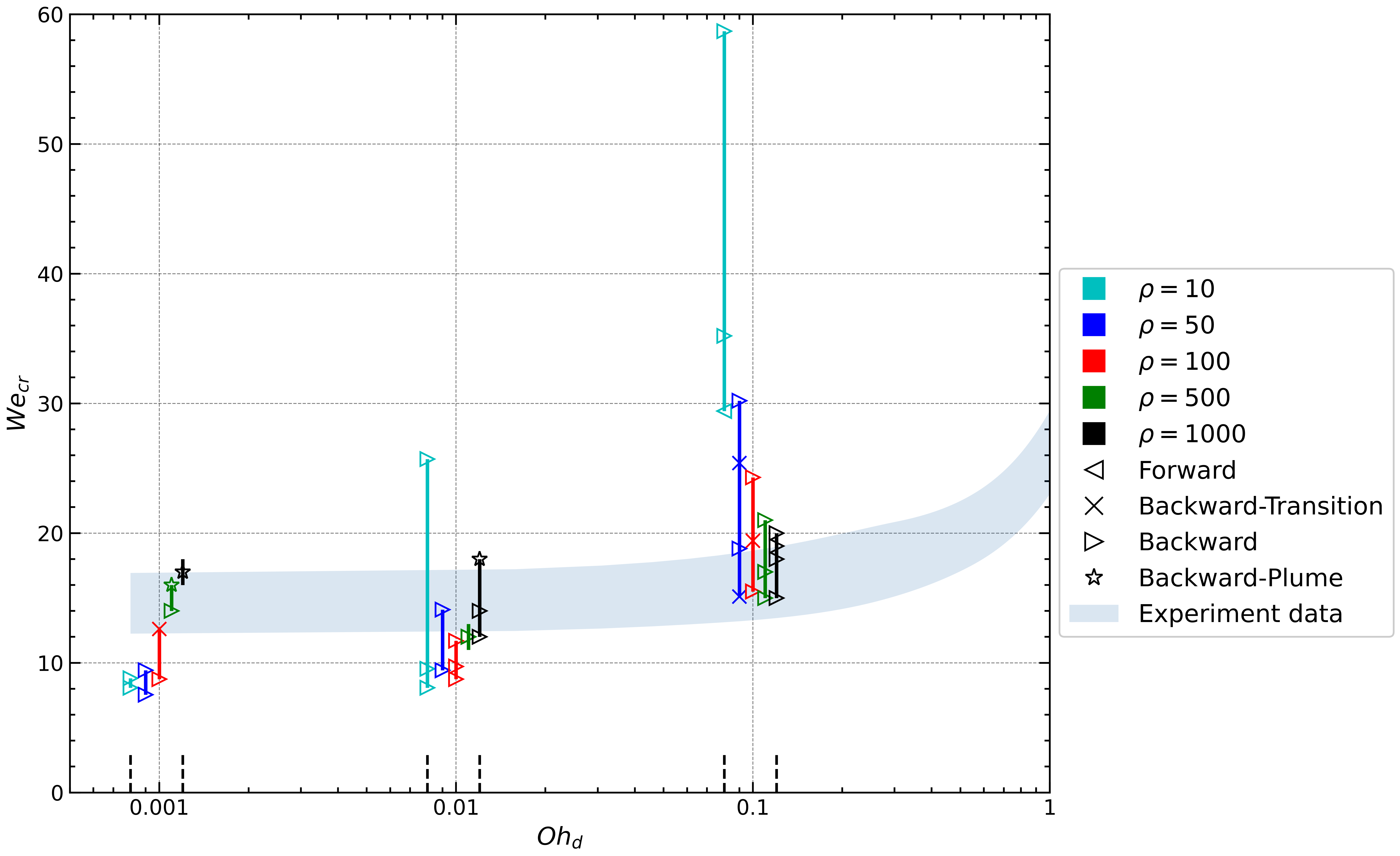
Figure 19: This figure plots $\mathit{We}_{cr}$’s dependence on $\mathit{Oh}_{d}$. Additionally, dependence on $\mathit{Oh}_{o}$ is represented using vertical lines, with their vertical extent representing corresponding variation in $\mathit{We}_{cr}$. Dependence on $\rho$ is shown through different colored vertical lines representing each $\rho$ value in the parameter space. Finally, specific markers are used to represent all critical breakup morphologies observed in the simulations.

On the basis of all the simulation results and figure 19, the following conclusions can be made:

1. All high $\rho$ ($\geq 500$) cases show $\mathit{We}_{cr}$ values very close to experimental data from existing literature. This is expected as historically most of the experimental work on Impulsive droplet breakup at critical conditions has been done for water-air analogous systems. Only cases with $\rho<500$ show any appreciable deviation from experimental results.

2. High $\rho$ ($\geq 500$) droplets show an almost constant $\mathit{We}_{cr}$ value for all $\mathit{Oh}_{d}\leq 0.1$. However, as $\rho$ decreases below 500, we start seeing larger variations in corresponding $\mathit{We}_{cr}$ values. The lowest $\rho$ cases show both the lowest $\mathit{We}_{cr}$ values (corresponding to the lowest $\mathit{Oh}_{d}$ values) as well as the highest $\mathit{We}_{cr}$ values (corresponding to the highest $\mathit{Oh}_{d}$ values) seen in figure 19.

3. Similarly, $\mathit{We}_{cr}$ shows larger variations on varying $\mathit{Oh}_{o}$ for lower $\rho$ values, as seen from the length of vertical lines in figure 19. A droplet with a large $\rho$ ($\geq 500$) has a large total inertia, and hence experiences larger relative velocities with the ambient flow. This makes ${\Delta P}_{drive}$ the dominant factor driving the deformation of the droplet in many cases. Even for cases with large external shear stresses on the droplet (for the largest $\mathit{Oh}_{o}$ values), once a clear rim has formed in the deformed droplet, local inertia variations take over the deformation process. Hence the lower inertia ($\rho$) droplets show the most sensitivity to changes in $\mathit{Oh}_{o}$. Furthermore, the intensity and location of downstream vortices interact more strongly with low $\rho$ droplets, and show little effect on droplets with large $\rho$. The only exception is when $\mathit{Re}_{0}$ is in the free-shear regime ($\mathit{Re}_{0}>10000$ (section 3.2).

4. Critical Breakup morphology shifts from a forward bag ($\rho=10$) to a backward-transition ($\rho=50,100$) (see figure 20) to a backward and backward-plume bag ($\rho\geq 500$) with increase in $\rho$. This shift in morphology from forward to backward bag is observed only for low $\mathit{Oh}_{o}$ values which show stronger downstream vortices and hence may provide additional local acceleration to periphery of low $\rho$ droplets, leading to a forward bag morphology. As $\rho$ increases, the droplet’s rim is expected to start lagging behind the droplet core at some point during its deformation, when local inertia of its rim becomes substantially larger than that of its core. On the other hand, large $\mathit{Oh}_{o}$ cases always show a backward bag breakup at critical conditions, even if the initial pancake formed is a forward pancake (for $\mathit{Oh}_{o}=0.1$). This is due to the downstream vortices being weak or non-existent for low $\mathit{Re}_{0}$ flows.

5. A decrease in $\mathit{Oh}_{d}$ motivates the critical breakup morphology to form a plume. This is seen for the lowest $\mathit{Oh}_{d}$ ($0.01,0.001$) and $\mathit{Oh}_{o}$ ($0.001,0.0001$) values, and for the largest $\rho$ ($500,1000$) droplets (star shaped marker in figure 19). Such droplets show an unstable plume at the upstream poles of their flat pancakes, which are also locations of maximum acceleration in the droplets. Hence, these plumes can be attributed to Rayleigh-Taylor instabilities, which are generated when accelerations are imposed on a fluid-fluid interface with a density discontinuity. Both low viscosity and larger density ratios motivate such instabilities (Villermaux, 2007; Guildenbecher et al., 2009; Jalaal & Mehravaran, 2014). Since the pancake for this non-dimensional set starts with a plume even for lower non-critical $\mathit{We}_{0}$ values, a plain backward bag breakup is not possible for such cases, and we always see a backward bag-plume breakup. On the other hand, all cases with higher $\mathit{Oh}_{d}$ values do not show any instabilities at the upstream pole and hence show a standard backward bag breakup under critical conditions.

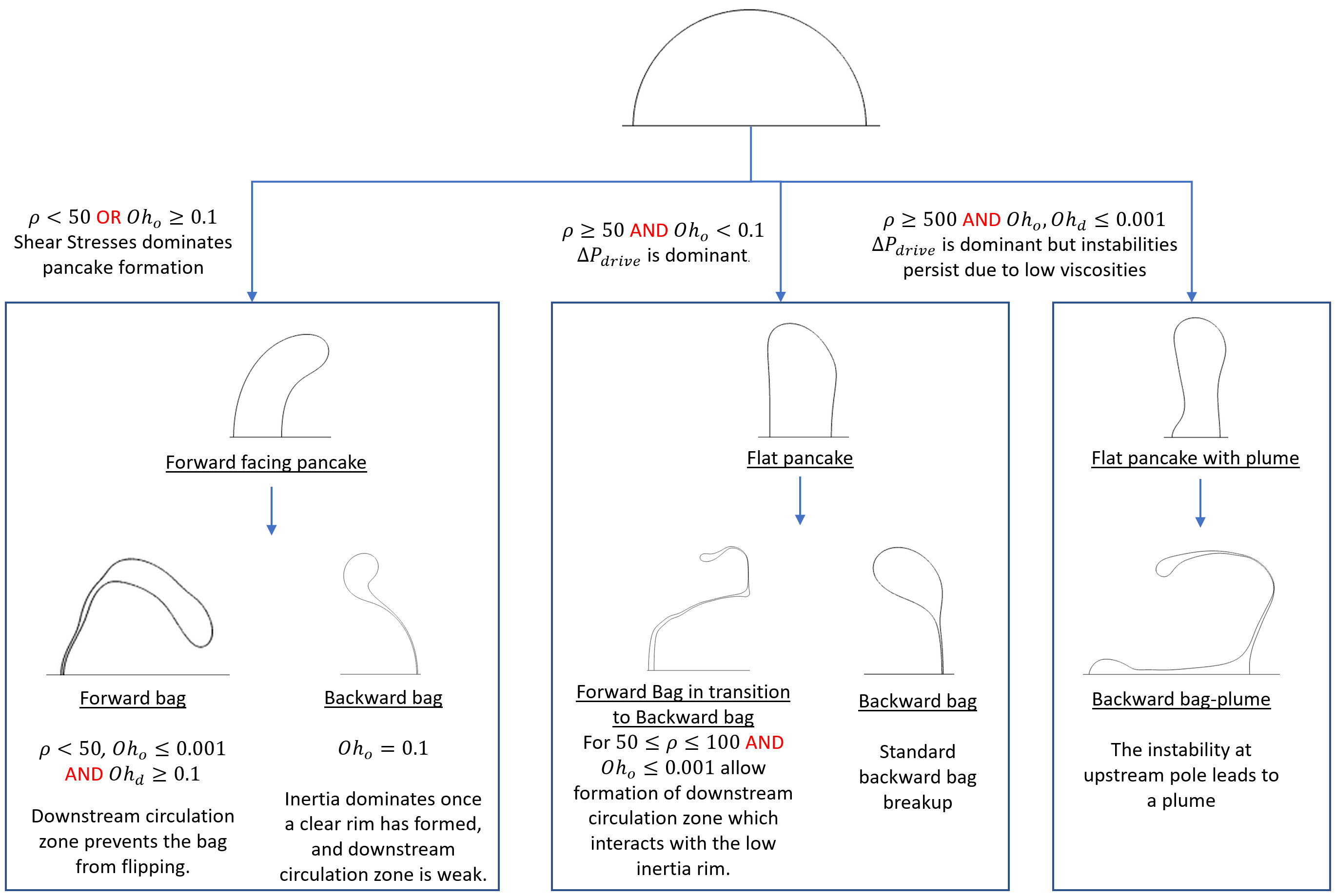
Figure 20: This phase diagram shows all deformation paths a spherical droplet under impulsive acceleration can take when breaking up critically. Under different non-dimensional parameter values, a spherical droplet can deform in to three types of pancakes, each of which further deform in to a breakup morphology.

The conclusions drawn from figure 19 show that the accepted idea of Critical Weber number being almost independent of drop Ohnesorge number for $\mathit{Oh}_{d}<0.1$, might not always hold, especially for systems which stray too far from rheological properties analogous to Water-Air. Furthermore, the critical breakup morphology need not necessarily be a backward bag breakup. Backward bag-plume and forward bag morphologies can be the critical morphologies for certain low $\rho$ and low $\mathit{Oh}_{o}$ cases.

Based on all the above findings, a phase diagram (figure 20) can be drawn that provides a detailed summary of all the deformation paths a spherical droplet can take towards critical breakup under impulsive acceleration. It is worth reiterating that all the breakup paths provided in the diagram are for their respective critical conditions, and hence the $\mathit{We}_{cr}$ values corresponding to different cases might not be the same. All the phase diagram informs us about is the type of pancake and corresponding general breakup morphology observed for a specific set of $\{\rho,\mathit{Oh}_{o},\mathit{Oh}_{d}\}$ at its $\mathit{We}_{cr}$. For information about the lowest $\mathit{We}$ required for achieving a non-vibrational breakup (i.e. $\mathit{We}_{cr}$), one may refer to figure 19.

For low $\rho$ or high $\mathit{Oh}_{o}$ values or both, the droplet first deforms into a forward pancake. From this stage, the fate of the bag depends on the balance between local inertia differences and strength and proximity of downstream vortices to the rim. The droplet continues its forward facing deformation and breaks up in a forward bag morphology at critical conditions if the downstream vortices overcome the inertia differences, which occurs when both $\mathit{Oh}_{o}$ and $\rho$ values are low. Alternatively for large $\rho$ cases, local inertia would dominate the deformation proceedings, especially once a clear rim has formed, and lead to the flipping of the bag from forward to backward bag, ultimately leading to a backward bag breakup morphology. This morphology is the most commonly observed critical breakup morphology in the explored parameter space.

When $\rho$ value is high and $\mathit{Oh}_{o}$ value is low, the droplet under critical conditions could deform into either a flat pancake or a flat pancake with a plume depending on whether $\rho$ and $\mathit{Oh}_{o}$ are at the extreme ends of the parameter space. The largest of $\rho$ values and the smallest of $\mathit{Oh}_{o}$ and $\mathit{Oh}_{d}$ values lead to a flat pancake with a plume. It can be hypothesized that the low viscosities of both outside and droplet fluids do not provide sufficient viscous dissipation to stabilize the jet ejected at the upstream pole (due to Rayleigh-Taylor instability) of the droplet. From this pancake shape, the only possible critical breakup morphology is a backward bag-plume breakup. All other intermediate cases form a flat pancake which can form either a forward-transition breakup (for intermediate $\rho$ values and low $\mathit{Oh}_{o}$ values) or a backward bag (for all the remaining cases). A forward-transition breakup is a forward bag with a flipped rim, i.e. a droplet which at its final moments gains enough mass in its rim to start the bag flipping process. As expected, this is observed for intermediate $\rho$ values where neither of local inertia differences or the effect of downstream vortices outright dominate the process.

4.2 Bag Inflation Characteristics

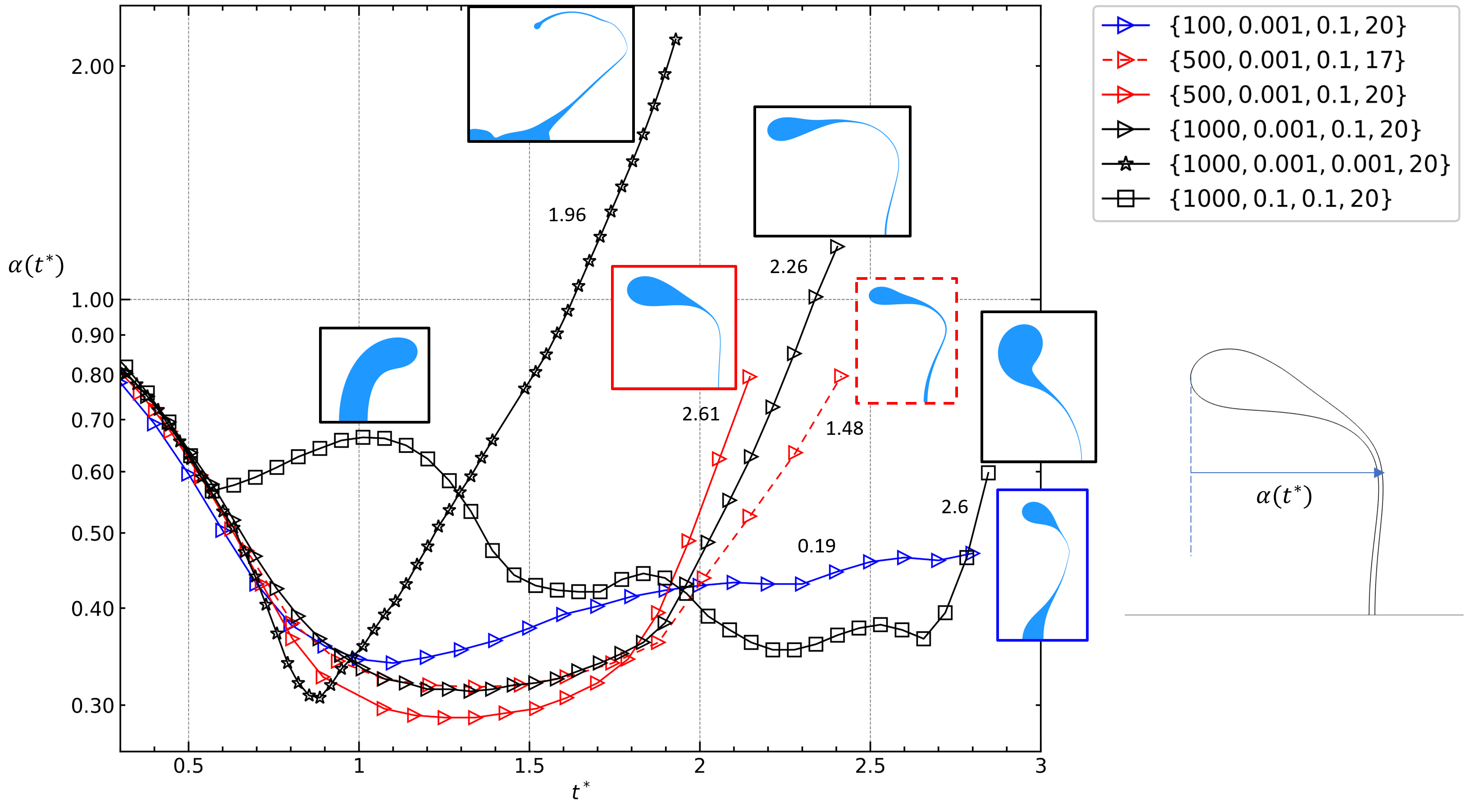
Figure 21: Bag inflation $\alpha(t^{*})$ with time $t^{*}$ is shown for some unique backward bag breakup cases. The non-dimensional parameter set for each case is of the form $\{\rho,\mathit{Oh}_{o},\mathit{Oh}_{d},\mathit{We}_{0}\}$. The cases plotted here include simple backward bags ($\{500,0.001,0.1,17\}$, $\{1000,0.1,0.1,20\}$ $\{1000,0.001,0.1,20\}$) and backward plume-bags ($\{100,0.001,0.1,20\}$, $\{500,0.001,0.1,20\}$, $\{1000,0.001,0.001,20\}$). In addition, $\{1000,0.1,0.1,20\}$ initially forms a forward pancake shape which then flips to backward bag. Through this plot, the effect of $\mathit{We}_{0}$, $\mathit{Oh}_{o}$ and $\rho$ on bag inflation rates is highlighted.

An understanding of the timescales involved in the inflation of bags in bag breakups is essential in correct estimation of bag burst timescales and effective centroid velocities for bag breakups. Villermaux & Bossa (2009) were the first to give an analytical description of bag inflation rates for the backward bag breakup. They found that the bag inflation amplitude increased exponentially with time with an exponent factor of 2 for an inviscid droplet. Kulkarni & Sojka (2014) extended the work of Villermaux & Bossa (2009) to include droplet viscosity and numerically obtained a similar exponential relationship for bag inflation, with $\mathit{Oh}_{d}$ as a factor signifying droplet viscosity. $\mathit{Oh}_{d}$ was found to have a very small impact on bag inflation rates. $\mathit{We}_{0}$ on the other hand has a more dramatic effect on the exponent factors governing inflation, with higher $\mathit{We}_{0}$ showing faster inflation rates. The current set of simulations present an opportunity to explore this property to parse the role of the relevant non-dimensional parameters on bag inflation.

The evolution of bag inflation with time for a few backward bag breakup cases is plotted in figure 21. For every plot, the droplet shows a decrease in $\alpha(t^{*})$ up until it reaches the end of pancake stage at $t^{*}\approx 1$, beyond which the droplet starts its inflation process. The only exception is the $\{1000,0.1,0.1,20\}$ case, which initially shows an increase in inflation due to achieving a forward pancake shape due to shear stresses dictating its internal flow. Bag inflation stage only starts at $t^{*}\approx 2.5$ for this case. Once firmly in bag inflation stage, all cases plotted here show an exponential growth $\alpha(t^{*})$ with time with a specific exponential growth factor, marked in figure 21 as numbers alongside each plot.

From the plots, a few interesting observations can be made. The $\{1000,0.001,0.001,20\}$ case, which has properties closest to a water-air droplet-ambient system, shows an inflation growth factor of 1.96, which is very close to the value that was analytically found by Villermaux & Bossa (2009), and was matched against a bag breakup experiment of a water droplet. Even though this case is a Backward-plume breakup, its inflation growth rate matches that of a simple bag, and is not affected by the presence of the plume.

For $\{500,0.001,0.1\}$ non-dimensional set, two Weber numbers are shown in the plot: $\mathit{We}_{0}=17,\,20$. It is observed that the higher $\mathit{We}_{0}$ droplet shows a higher exponent factor dictating its exponential growth in $\alpha(t^{*})$. This is an expected observation since the overall deformation rate is also higher for a higher $\mathit{We}_{0}$ case, owing to the lower surface tension forces relative to the dynamic pressure forces driving the droplet’s deformation. Hence, the same amount of energy (supplied to the droplet by the external forces) should lead to a larger change in interface area due to a lower surface tension.

We also observe that the $\rho=100$ case shows a dramatically lower inflation growth rate compared to an analogous $\rho=500$ or $\rho=1000$ cases. This may be attributed to the higher centroid velocities seen for the low $\rho$ case, which results in a decrease in effective Weber number, and hence a higher surface tension relative to the effective dynamic pressure forcing.

Droplet and ambient viscosities appear to have an inverse effect on bag inflation rates. Among the three $\rho=1000$ cases shown in the plot, the higher droplet and ambient Ohnesorge number cases show the larger rates of exponential growth of $\alpha(t^{*})$.

More generally, figure 21 shows that $t\approx\tau$ (or $t^{*}\approx 1$) (equation 1) is a good representative timescale for the start of bag inflation process. This observation matches with the Aspect ratio plots shown in figures 8 and 12 in which the pancake formation stage almost always ends at $t^{*}\approx 1$. If the aerodynamic forces acting on a droplet are large enough to initiate bag inflation in its pancake, it is expected for the droplet to go on to or be very close to fragmentation. Hence, we hypothesize that the balance of all the forces acting on a droplet (aerodynamic forces driving its deformation, and capillary and viscous forces resisting it) at this stage, i.e., at the end of its pancake formation and start of its bag inflation, is representative of the overall fragmentation stability of the droplet. We will use this timescale to obtain a better estimate of the effective aerodynamic forces on the droplet in the next section.

4.3 A parameter for Prediction of Breakup Threshold

Most previous works have characterized the threshold for impulsive breakup of spherical droplets using the Weber number based on initial velocity deficit with the ambient medium $\mathit{We}_{0}=\rho_{o}V_{0}^{2}D/\sigma$). For all cases with properties analogous to Water-Air system, i.e., $\rho>500$, $\mathit{Oh}_{o}<0.01$ and $\mathit{Oh}_{d}<0.1$, critical breakup does consistently occur at a critical Weber number of $\mathit{We}_{cr}\approx 14$. However, as has been discovered and exhaustively described through the simulation results in the previous sections (summarized succinctly in figures 19 and 20), different cases which stray away from the non-dimensional space described by Water-air systems, do not show the same threshold Weber number value. Substantially higher $\mathit{We}_{cr}$ values are observed for case with low density ratios and high Ohnesorge numbers. Weber number $\mathit{We}_{0}$ represents the ratio of the pressure forces applied on a droplet’s surface by the ambient medium, based on its initial relative velocity, motivating its deformation to the surface tension acting against any change in surface energy. However, a droplet’s deformation also depends on the viscous forces applied by the surrounding flow, its inertia and hence its acceleration, and the viscous dissipation against its internal fluid flow. These effects have been explained in detail in section 3 through simulations for varying $\mathit{Oh}_{o}$, $\mathit{Oh}_{d}$ and $\rho$ values respectively. $\mathit{We}_{0}$ hence does not capture the role of all the factors relevant in the droplet deformation process. We hence aim to construct a new non-dimensional group which aggregates the effect of all the parameters, namely $\mathit{We}_{0}$, $\mathit{Oh}_{o}$, $\mathit{Oh}_{d}$ and $\rho$ and shows a consistent critical value demarcating the threshold of breakup under impulsive acceleration for the complete parameter space studied in this work.

Let us assume that this new non-dimensional number, denoted by $C_{\mathit{breakup}}$, is a function of all the dimensional variables involved in the breakup process (15). There are $3$ independent dimensions in the problem. Hence, through Buckingham-Pi analysis, we can obtain at most $4$ independent non-dimensional numbers. $4$ non-dimensional numbers relevant to this problem have already been defined in section 2.1, namely $\rho$, $\mathit{Oh}_{o}$, $\mathit{Oh}_{d}$, and $\mathit{We}_{0}$. So, it is expected for $C_{\mathit{breakup}}$ to develop into a function of these parameters (16).

$$C_{\mathit{breakup}}=f(V_{0},D,\rho_{o},\rho_{d},\mu_{o},\mu_{d},\sigma)$$ (15)

$$C_{\mathit{breakup}}=f(\mathit{We}_{0},\rho,\mathit{Oh}_{o},\mathit{Oh}_{d})$$ (16)

To obtain $C_{\mathit{breakup}}$, we follow a procedure similar to that employed by Blackwell et al. (2015) (see section IV), where they use the ratio of the forces antagonistic to each other to define a non-dimensional group. We utilize a similar hypothesis to define $C_{\mathit{breakup}}$, i.e., the competition between the forces driving droplet deformation and the forces resisting the process, to define the criteria for breakup threshold. This balance can be represented as a ratio of the respective magnitudes of the forces as follows:

$$C_{\mathit{breakup}}=\frac{\textrm{Forces driving droplet deformation}}{\textrm{Forces resisting droplet deformation}}$$ (17)

Hence to obtain $C_{\mathit{breakup}}$, all the force scales relevant in the droplet deformation process would be required. This includes obtaining scales for the aerodynamic stresses applied by the ambient flow, and the surface tension and viscous stresses developed at the interface and inside the droplet respectively.

A droplet under impulsive acceleration starts at zero velocity and then asymptotically accelerates towards a maximum velocity equal to the ambient flow (given that the droplet is still intact). This acceleration is driven by the drag forces applied the aerodynamic stresses on the droplet interface. The same aerodynamic forces also drive the droplet’s deformation. These forces are composed of dynamic pressure ($\tau_{p}$) and viscous stresses ($\tau_{\mu_{o}}$), where magnitudes of both are dictated by the instantaneous flow Reynolds number (5) and relative velocity with the ambient medium $V_{\mathit{rel}}$. Let us assume that a scale for the total force per unit droplet surface area is given by $\tau_{\mathit{aero}}$. $\tau_{\mathit{aero}}$ can be scaled as:

$$\tau_{\mathit{aero}}=\left(\tau_{p}+\tau_{\mu_{o}}\right)\propto\rho_{o}V_{\mathit{rel}}^{2}$$ (18)

As the droplet continues accelerating, its relative velocity with respect to the ambient medium continues to decrease, which reduces both pressure and viscous stresses. For water-air systems where $\mathit{Oh}_{o}$ is low and $\rho$ is high, the droplet does not show any significant accelerations and $V_{\mathit{rel}}$ remains almost equal to the initial relative velocity of $V_{0}$ for the whole breakup process. For such cases, $V_{\mathit{rel}}$ can be assumed to be equal to $V_{0}$. On the other hand, if the droplet shows significant accelerations and gains velocities which are a substantial fraction of $V_{0}$, which is the case for low $\rho$ or high $\mathit{Oh}_{o}$ cases, $V_{\mathit{rel}}$ cannot be assumed to be equal to $V_{0}$ anymore. Hence, it becomes essential to derive a scaling for $V_{\mathit{rel}}$ which is valid for the whole parameter space. For this purpose, we make use of the drag equation for a sphere (19) to obtain a scale for the acceleration experienced by the droplet.

$$F_{\mathit{drag}}=0.5C_{D}\rho_{o}V_{\mathit{rel}}^{2}A$$ (19)

At $t=0$ when the droplet is at rest:

$$F_{\mathit{drag}}(t=0)=0.5C_{D0}\rho_{o}V_{0}^{2}\frac{\pi}{4}D^{2} =\frac{\pi}{8}C_{D0}\rho_{o}V_{0}^{2}D^{2}$$ (20a)

$$\rho_{d}\frac{\pi}{6}D^{3}a_{\mathit{drop}} =\frac{\pi}{8}C_{D0}\rho_{o}V_{0}^{2}D^{2}$$ (20b)

$$a_{0} =\frac{3}{4}\frac{1}{\rho D}C_{D0}V_{0}^{2}$$ (20c)

Using this acceleration scale $a_{0}$ found from the droplet’s acceleration at $t=0$, we obtain a scale for the droplet’s centroid velocity by finding its velocity after a time equal to its deformation timescale $\tau$ (1) has elapsed (section 4.2), denoted as $V_{\tau}$.

$$V_{\tau}\propto\tau a_{0}\propto\left(\frac{D}{V_{0}}\sqrt{\rho}\right)\;\frac{3}{4}\frac{1}{\rho D}C_{D0}V_{0}^{2}=\frac{3}{4}\frac{C_{D0}}{\sqrt{\rho}}V_{0}$$ (21)

A scale for $V_{\mathit{rel}}$ can be obtained by evaluating $V_{0}-V_{\tau}$:

$$V_{\mathit{rel}}\propto V_{0}\left(1-\frac{3}{4}\frac{C_{D0}}{\sqrt{\rho}}\right)$$ (22)

$$V_{\mathit{rel}}\propto K_{v}V_{0}$$ (23)

In figures 8 and 12, we observe that the droplet’s centroid velocity decreases with an increase in $\rho$ and decrease in $\mathit{Oh}_{o}$. These observations are in line with the relative velocity scale obtained in equation 23, where $C_{D0}$ is a function of $\mathit{Re}_{0}=\sqrt{\mathit{We}_{0}}/\mathit{Oh}_{o}$. Any increase in the ratio between $C_{D0}$ and $\sqrt{\rho}$ leads to a decrease in $V_{\mathit{rel}}$. It is also important to note that the use of deformation timescale in estimating the velocity scale implicitly imports the assumption that the droplet flattens into a pancake before blowing into a bag. Hence, we expect $C_{\mathit{breakup}}$ to correctly capture the threshold for droplets whose critical breakup morphology is a bag breakup.

We can finally obtain a scale for the aerodynamic stress applied by the ambient medium on the droplet surface:

$$\tau_{\mathit{aero}} \propto\rho_{o}K_{v}^{2}V_{o}^{2}$$ (24a)

$$\propto K_{v}^{2}\frac{\rho_{o}V_{o}^{2}D}{\sigma}\frac{\sigma}{D}$$ (24b)

$$\tau_{\mathit{aero}} \propto K_{v}^{2}\mathit{We}_{0}\tau_{\sigma}$$ (24c)

Here $\tau_{\sigma}$ is a scale representing surface tension force per unit area of the droplet.

The dynamic pressure acting on the droplet surface leads to a response from the surface tension of the droplet-ambient interface by developing changes in the curvature and area of the interface. The viscous stresses instead draw a response from the droplet fluid by setting a flow inside the droplet. Hence, surface tension force per unit area $\tau_{\sigma}$ and the viscous forces per unit area $\tau_{\mu_{d}}$ provide resistance to droplet deformation. Based on the work of Hinze (1955), we can provide scales of these stresses as follows:

$$\tau_{\sigma}=\frac{\sigma}{D}$$ (25)

$$\tau_{\mu_{d}} \propto\mu_{d}\frac{\sqrt{\tau_{\mathit{aero}}/\rho_{d}}}{D}$$ (26a)

$$\propto\mu_{d}\dfrac{\sqrt{\rho_{d}\sigma D}}{\sqrt{\rho_{d}\sigma D}}\sqrt{\frac{K_{v}^{2}\mathit{We}_{0}\tau_{\sigma}}{\rho_{d}D^{2}}}$$ (26b)

$$\propto\dfrac{\mu_{d}}{\sqrt{\rho_{d}\sigma D}}\sqrt{\frac{K_{v}^{2}\mathit{We}_{0}\tau_{\sigma}\rho_{d}\sigma D}{\rho_{d}D^{2}}}$$ (26c)

$$\propto\mathit{Oh}_{d}\sqrt{K_{v}^{2}\mathit{We}_{0}\tau_{\sigma}^{2}}$$ (26d)

$$\tau_{\mu_{d}} \propto\mathit{Oh}_{d}K_{v}\sqrt{\mathit{We}_{0}}\;\tau_{\sigma}$$ (26e)

Equation 17 can now be rewritten incorporating aerodynamic stresses (18, surface tension stress (25), and viscous resistance in droplet fluid (26e).

$$C_{\mathit{breakup}}=\frac{\tau_{\mathit{aero}}A_{\mathit{aero}}}{\tau_{\sigma}A_{\sigma}+\tau_{\mu_{d}}A_{\mu_{d}}}$$ (27)

All three area scales for the three forces have the same value of $D^{2}$ and hence $C_{\mathit{breakup}}$ can be simplified to:

$$C_{\mathit{breakup}} =\frac{\tau_{\mathit{aero}}}{\tau_{\sigma}+\tau_{\mu_{d}}}$$ (28a)

$$C_{\mathit{breakup}} =\frac{K_{v}^{2}\mathit{We}_{0}\tau_{\sigma}}{\tau_{\sigma}+\mathit{Oh}_{d}K_{v}\sqrt{\mathit{We}_{0}}\;\tau_{\sigma}}$$ (28b)

which finally results in:

$$C_{\mathit{breakup}}=\frac{K_{v}^{2}\mathit{We}_{0}}{1+\mathit{Oh}_{d}K_{v}\sqrt{\mathit{We}_{0}}}$$ (29)

given:

$$K_{v}=\left(1-\frac{3}{4}\frac{C_{D0}}{\sqrt{\rho}}\right)$$ (30)

To replicate a Water-Air analogous system, if we ignore the effect of droplet viscosity by assuming $\mathit{Oh}_{d}<<1$, and assume the density ratio $\rho>500$ to be much larger than $C_{D0}$ (which is $\approx 1$ for large $\mathit{Re}_{0}$), $C_{\mathit{breakup}}$ simplifies to:

$$C_{\mathit{breakup}}\approx\mathit{We}_{0}$$ (31)

This result (31) coincides with the choice of a constant $\mathit{We}_{0}$ ($\approx 14$) as the critical breakup threshold criteria ($\mathit{We}_{cr}$) in current literature. It is only when droplet fluid viscosity starts to become significant, or the density contrast with respect to the ambient medium starts to become small, when $\mathit{We}_{0}$ starts to diverge from $C_{\mathit{breakup}}$.

Figure 22: This figure shows an alternate version of figure 19 where instead of $\mathit{We}_{cr}$, the variation of $C_{\mathit{breakup}}$ with respect to $\rho$, $\mathit{Oh}_{o}$, and $\mathit{Oh}_{d}$ is plotted. In addition to simulation data, all available experimental data in the relevant non-dimensional space for critical bag breakup (plotted in figure 1) is also plotted here for reference.

For obtaining of $C_{\mathit{breakup}}$ using 29, an explicit equation for drag coefficient is required. We use the relationship (32) provided by Turton & Levenspiel (1986). Note that $C_{D0}$ is a function of $\mathit{Re}_{0}$ but can also be expressed in terms of $\mathit{Oh}_{o}$ and $\mathit{We}_{0}$ since $\mathit{Re}_{0}=\sqrt{\mathit{We}_{0}}/\mathit{Oh}_{o}$.

$$C_{D0}=\frac{24}{\mathit{Re}_{0}}\left(1+0.173\mathit{Re}_{0}^{0.657}\right)+\frac{0.413}{1+16300\mathit{Re}_{0}^{-1.09}}$$ (32)

The $\mathit{We}_{cr}$ vs $\mathit{Oh}_{d}$ plot in figure 19 is re-plotted using $C_{\mathit{breakup}}$ (29) in the y-axis in figure 22. When scaled according to this new non-dimensional parameter, almost all simulation points move to a narrow range of $6<C_{\mathit{breakup}}<18$, when compared to $7<\mathit{We}_{cr}<60$ in the former plot. The highest $\mathit{We}_{cr}$ cases corresponding to $\mathit{Oh}_{d},\mathit{Oh}_{o}=0.1$ and $\rho=10,50$ in figure 19 when plotted according to 29 achieve substantially lower threshold values, much more in line with the $C_{\mathit{breakup}}$ values obtained for other simulation cases. It is also observed that the backward bag-plume breakup cases and the lowest density ratio cases show relatively the largest variance in $C_{\mathit{breakup}}$ values even in this updated plot. We also plot $C_{\mathit{breakup}}$ values of all the available experimental data for critical backward bag breakup as a set of reference data for the plot. As expected, the experimental data remains bound within a narrow extent of $C_{\mathit{breakup}}$ values, similar to its $\mathit{We}_{cr}$ analogue.

The $C_{\mathit{breakup}}$ values do start to drop off as we approach larger and larger $\mathit{Oh}_{d}$ values, i.e., $C_{\mathit{breakup}}$ appears to overestimate the effort required to achieve critical breakup in very high $\mathit{Oh}_{d}$ droplets compared to experiments. This is in line with the observations in previous experimental works (Hinze, 1955; Hsiang & Faeth, 1995) where it was observed that bag breakup becomes progressively difficult for higher drop Ohnesorge numbers and ultimately stops happening for $\mathit{Oh}_{d}>2$. Other breakup modes such as Multimode and sheet thinning become the critical breakup modes for very high $\mathit{Oh}_{d}$ values. The inherent assumption in the derivation of $C_{\mathit{breakup}}$ was to assume that critical breakup morphology is a bag breakup, i.e., a droplet first flattens into a pancake which then blows in to a bag. Any major deviation from this general breakup mechanism is expected to drastically change the deformation and breakup physics of such droplets. Hence, as $\mathit{Oh}_{d}$ increases past $0.1$, physics related to multimode and sheet thinning breakups start to become significant and hence must be considered in the derivation of any parameter attempting to define the critical breakup criteria.

Another factor worth consideration is the initial Reynolds number required (i.e., $\mathit{Re}_{0}=\sqrt{\mathit{We}_{0}}/\mathit{Oh}_{o}$) for the very large $\mathit{We}_{0}$ values to show a breakup for high $\mathit{Oh}_{d}$ droplets. For very large $\mathit{We}_{0}$ values, very large $\mathit{Re}_{0}$ values are expected which would make the external flow more chaotic, which can have an major effect on the pressure forces experienced by the droplet, its interaction with downstream vortices, and intensity of surface waves (section 3.2). These effects have not been taken into consideration in our derivation of $C_{\mathit{breakup}}$.

For the non-dimensional parameter space in consideration in the current work, $C_{\mathit{breakup}}$ very well captures the dominant physics and succeeds in compressing the rather large variance in $\mathit{We}_{cr}$ values observed due to very low $\rho$ and high $\mathit{Oh}_{d}$ and $\mathit{Oh}_{o}$ values. Hence for the purposes of the work, $C_{\mathit{breakup}}$ fulfills our requirements.

5 Conclusions

The current work aimed to clarify two major questions: 1. Effect of each of $\mathit{We}_{0}$, $\rho$, $\mathit{Oh}_{o}$ and $\mathit{Oh}_{d}$ on droplet deformation and breakup characteristics, at or near its $\mathit{We}_{cr}$ and for rheological properties vastly different from commonly available Water-Air systems; and 2. Effect of these non-dimensional parameters on droplet critical breakup morphology. As has been explained extensively in section 1, most of the currently accepted ideas on critical secondary atomization such as independence of $\mathit{We}_{cr}$ with respect to $\mathit{Oh}_{d}$ given its small, or the critical breakup morphology being solely a backward bag, etc. originate from experimental works done for a small parametric space occupied by Water-Air analogous systems. The current work aimed to shed some light on these accepted ideas and provide a more complete picture on the process of secondary atomization of Newtonian droplets. For this purpose, a parametric sweep across all the involved non-dimensional parameters, i.e. $\{\rho,\mathit{Oh}_{o},\mathit{Oh}_{d}\}$ (section 2.4) was performed using axisymmetric simulations on Basilisk, with $\mathit{We}_{0}$ values increased until a non-vibrational (critical) breakup was achieved for a given $\{\rho,\mathit{Oh}_{o},\mathit{Oh}_{d}\}$ set. From the subsequently obtained simulation results, the effect of each of the non-dimensional parameters on a droplet’s deformation were characterized and related to the external forces acting on the droplet and the corresponding internal flows (section 3). $\mathit{We}_{cr}$ for the parameter space was obtained and plotted against $\mathit{Oh}_{d}$ (figure 19) to recreate the plot presented in Hsiang & Faeth (1995). On the basis of all the analysis performed on the simulation results, a phase diagram (figure 20) was constructed describing the various deformation pathways a spherical droplet under impulsive acceleration would take depending on its rheological properties. The simulations also allowed us to explore bag inflation characteristics for backward bag breakups for a greater parameter space, and extract some general conclusions on the associated timescales and growth rates. Additionally, $t^{*}\approx 1$ was found to be a good measure for timescale required for the initiation of bag inflation. Finally, a non-dimensional parameter ($C_{\mathit{breakup}}$) was derived to provide a more complete alternative to Weber number as an indicator of droplet threshold criteria in the dimensional space of current work by capturing the effects of all three studied non-dimensional parameters, i.e., $\rho$, $\mathit{Oh}_{o}$, and $\mathit{Oh}_{d}$ on droplet deformation and breakup.

6 Acknowledgement

Computational resources provided by the Covid-19 HPC Consortium through time on Blue Waters (NCSA) were used for the simulations. S.D. and A.P.’s participation was supported by the DOE Office of Science through the National Virtual Biotechnology Laboratory (NVBL), a consortium of DOE national laboratories focused on response to COVID-19, with funding provided by the Coronavirus CARES Act.

References

- Blackwell et al. (2015) Blackwell, Brendan C., Deetjen, Marc E., Gaudio, Joseph E. & Ewoldt, Randy H. 2015 Sticking and splashing in yield-stress fluid drop impacts on coated surfaces. Physics of Fluids 27 (4), 043101, publisher: American Institute of Physics.
- Brackbill et al. (1992) Brackbill, J. U, Kothe, D. B & Zemach, C 1992 A continuum method for modeling surface tension. Journal of Computational Physics 100 (2), 335–354.
- Bremond & Villermaux (2005) Bremond, N. & Villermaux, E. 2005 Bursting thin liquid films. Journal of Fluid Mechanics 524, 121–130, publisher: Cambridge University Press.
- Cao et al. (2007) Cao, Xian Kui, Sun, Zhi Gang, Li, Wei Feng, Liu, Hai Feng & Yu, Zun Hong 2007 A new breakup regime of liquid drops identified in a continuous and uniform air jet flow. Physics of Fluids 19 (5), 057103.
- Dai & Faeth (2001) Dai, Z. & Faeth, G. M. 2001 Temporal properties of secondary drop breakup in the multimode breakup regime. International Journal of Multiphase Flow 27 (2), 217–236.
- Dorschner et al. (2020) Dorschner, Benedikt, Biasiori-Poulanges, Luc, Schmidmayer, Kevin, El-Rabii, Hazem & Colonius, Tim 2020 On the formation and recurrent shedding of ligaments in droplet aerobreakup. Journal of Fluid Mechanics 904, publisher: Cambridge University Press.
- Flock et al. (2012) Flock, A.K., Guildenbecher, D.R., Chen, J., Sojka, P.E. & Bauer, H.-J. 2012 Experimental statistics of droplet trajectory and air flow during aerodynamic fragmentation of liquid drops. International Journal of Multiphase Flow 47, 37–49, publisher: Pergamon.
- Forouzi Feshalami et al. (2022) Forouzi Feshalami, Behzad, He, Shuisheng, Scarano, Fulvio, Gan, Lian & Morton, Chris 2022 A review of experiments on stationary bluff body wakes. Physics of Fluids 34 (1), 011301, publisher: American Institute of Physics.
- Francois et al. (2006) Francois, Marianne M., Cummins, Sharen J., Dendy, Edward D., Kothe, Douglas B., Sicilian, James M. & Williams, Matthew W. 2006 A balanced-force algorithm for continuous and sharp interfacial surface tension models within a volume tracking framework. Journal of Computational Physics 213 (1), 141–173.
- Fuster et al. (2009) Fuster, Daniel, Agbaglah, Gilou, Josserand, Christophe, Popinet, Stéphane & Zaleski, Stéphane 2009 Numerical simulation of droplets, bubbles and waves: State of the art. Fluid Dynamics Research 41 (6), 065001.
- Gelfand (1996) Gelfand, B E 1996 Droplet breakup phenomena in flows with velocity lag. Progress in Energy and Combustion Science 22 (3), 201–265.
- Goodridge et al. (1997) Goodridge, Christopher L., Shi, W. Tao, Hentschel, H. G. E. & Lathrop, Daniel P. 1997 Viscous effects in droplet-ejecting capillary waves. Physical Review E 56 (1), 472–475, publisher: American Physical Society.
- Guildenbecher et al. (2009) Guildenbecher, D. R., López-Rivera, C. & Sojka, P. E. 2009 Secondary atomization. Experiments in Fluids 46 (3), 371–402, publisher: Springer.
- Han & Tryggvason (2001) Han, Jaehoon & Tryggvason, Gretar 2001 Secondary breakup of a axisymmetric liquid drops. II. Impulsive acceleration. Physics of Fluids 13 (6), 1554–1565, publisher: American Institute of PhysicsAIP.
- Hinze (1949) Hinze, J. O. 1949 Critical speeds and sizes of liquid globules. Applied Scientific Research 1 (1), 273–288.
- Hinze (1955) Hinze, J. O. 1955 Fundamentals of the hydrodynamic mechanism of splitting in dispersion processes. AIChE Journal 1 (3), 289–295.
- Hsiang & Faeth (1995) Hsiang, LP & Faeth, GM 1995 Drop deformation and breakup due to shock wave and steady disturbances. International Journal of Multiphase Flow 21 (4), 545–560.
- Hsiang & Faeth (1992) Hsiang, L. P. & Faeth, G. M. 1992 Near-limit drop deformation and secondary breakup. International Journal of Multiphase Flow 18 (5), 635–652.
- Jackiw & Ashgriz (2021) Jackiw, Isaac M. & Ashgriz, Nasser 2021 On aerodynamic droplet breakup. Journal of Fluid Mechanics 913 (A33), 1–46.
- Jain et al. (2015) Jain, Mohit, Prakash, R. Surya, Tomar, Gaurav & Ravikrishna, R. V. 2015 Secondary breakup of a drop at moderate Weber numbers. Proceedings of the Royal Society A: Mathematical, Physical and Engineering Sciences 471 (2177), publisher: Royal Society of London.
- Jain et al. (2019) Jain, Suhas S., Tyagi, Neha, Prakash, R. Surya, Ravikrishna, R. V. & Tomar, Gaurav 2019 Secondary breakup of drops at moderate Weber numbers: Effect of Density ratio and Reynolds number. International Journal of Multiphase Flow 117, 25–41, arXiv: 1803.02989 Publisher: Elsevier Ltd.
- Jalaal & Mehravaran (2012) Jalaal, M. & Mehravaran, K. 2012 Fragmentation of falling liquid droplets in bag breakup mode. International Journal of Multiphase Flow 47, 115–132, publisher: Pergamon.
- Jalaal & Mehravaran (2014) Jalaal, M. & Mehravaran, K. 2014 Transient growth of droplet instabilities in a stream. Physics of Fluids 26 (1), 012101, publisher: American Institute of Physics.
- Karam & Bellinger (1968) Karam, H. J. & Bellinger, J. C. 1968 Deformation and Breakup of Liquid Droplets in a Simple Shear Field. Industrial & Engineering Chemistry Fundamentals 7 (4), 576–581, publisher: American Chemical Society.
- Khosla & Smith (2006) Khosla, Sachin & Smith, Clifford E 2006 Detailed Understanding of Drop Atomization by Gas Crossflow Using the Volume of Fluid Method. In ILASS Americas, 19th Annual Conference on Liquid Atomization and Spray Systems. Institute for Liquid Atomization and Spray Systems.
- Krzeczkowski (1980) Krzeczkowski, Stefan A. 1980 Measurement of liquid droplet disintegration mechanisms. International Journal of Multiphase Flow 6 (3), 227–239, publisher: Pergamon.
- Kulkarni & Sojka (2014) Kulkarni, V. & Sojka, P. E. 2014 Bag breakup of low viscosity drops in the presence of a continuous air jet. Physics of Fluids 26 (7), 072103, publisher: American Institute of Physics.
- Lozano et al. (1998) Lozano, Antonio, Garcı?a-Olivares, Antonio & Dopazo, César 1998 The instability growth leading to a liquid sheet breakup. Physics of Fluids 10 (9), 2188–2197.
- Marcotte & Zaleski (2019) Marcotte, Florence & Zaleski, Stéphane 2019 Density contrast matters for drop fragmentation thresholds at low Ohnesorge number. Physical Review Fluids 4 (10), 103604, publisher: American Physical Society.
- Pilch & Erdman (1987) Pilch, M. & Erdman, C.A. 1987 Use of breakup time data and velocity history data to predict the maximum size of stable fragments for acceleration-induced breakup of a liquid drop. International Journal of Multiphase Flow 13 (6), 741–757, publisher: Pergamon.
- Popinet (2003) Popinet, Stéphane 2003 Gerris: a tree-based adaptive solver for the incompressible Euler equations in complex geometries. Journal of Computational Physics 190 (2), 572–600, publisher: Academic Press.
- Popinet (2009) Popinet, Stéphane 2009 An accurate adaptive solver for surface-tension-driven interfacial flows. Journal of Computational Physics 228 (16), 5838–5866, publisher: Academic Press.
- Popinet (2015) Popinet, Stéphane 2015 A quadtree-adaptive multigrid solver for the Serre–Green–Naghdi equations. Journal of Computational Physics 302, 336–358, publisher: Elsevier.
- Pruppacher & Beard (1970) Pruppacher, H. R. & Beard, K. V. 1970 A wind tunnel investigation of the internal circulation and shape of water drops falling at terminal velocity in air. Quarterly Journal of the Royal Meteorological Society 96 (408), 247–256, publisher: John Wiley & Sons, Ltd.
- Rimbert et al. (2020) Rimbert, N., Castrillon Escobar, S., Meignen, R., Hadj-Achour, M. & Gradeck, M. 2020 Spheroidal droplet deformation, oscillation and breakup in uniform outer flow. Journal of Fluid Mechanics 904, 15–16, publisher: Cambridge University Press.
- Szakáll et al. (2009) Szakáll, Mikloós, Diehl, Karoline & Mitra, Subir K. 2009 A wind tunnel study on the shape, oscillation, and internal circulation of large raindrops with sizes between 2.5 and 7.5 mm. Journal of the Atmospheric Sciences 66 (3), 755–765.
- Theofanous (2011) Theofanous, T.G. 2011 Aerobreakup of Newtonian and Viscoelastic Liquids. Annual Review of Fluid Mechanics 43 (1), 661–690, _eprint: https://doi.org/10.1146/annurev-fluid-122109-160638.
- Theofanous et al. (2004) Theofanous, T. G., Li, G. J. & Dinh, T. N. 2004 Aerobreakup in Rarefied Supersonic Gas Flows. Journal of Fluids Engineering 126 (4), 516–527.
- Torrey et al. (1985) Torrey, M. D., Cloutman, L. D., Mjolsness, R. C. & Hirt, C. W. 1985 NASA-VOF2D: a computer program for incompressible flows with free surfaces. NASA STI/Recon Technical Report N 86, 30116, aDS Bibcode: 1985STIN…8630116T.
- Turton & Levenspiel (1986) Turton, R. & Levenspiel, O. 1986 A short note on the drag correlation for spheres. Powder Technology 47 (1), 83–86.
- Villermaux (2007) Villermaux, E. 2007 Fragmentation. Annual Review of Fluid Mechanics 39 (1), 419–446, publisher: Annual Reviews.
- Villermaux & Bossa (2009) Villermaux, Emmanuel & Bossa, Benjamin 2009 Single-drop fragmentation determines size distribution of raindrops. Nature Physics 5 (9), 697–702, publisher: Nature Publishing Group.
- Wierzba (1990) Wierzba, A. 1990 Deformation and breakup of liquid drops in a gas stream at nearly critical Weber numbers. Experiments in Fluids 9 (1), 59–64.
- Zhao et al. (2011) Zhao, Hui, Liu, Hai Feng, Cao, Xian Kui, Li, Wei Feng & Xu, Jian Liang 2011 Breakup characteristics of liquid drops in bag regime by a continuous and uniform air jet flow. International Journal of Multiphase Flow 37 (5), 530–534, publisher: Pergamon.