Factor-guided functional PCA
for high-dimensional functional data

Abstract

The literature on high-dimensional functional data focuses on either the dependence over time or the correlation among functional variables. In this paper, we propose a factor-guided functional principal component analysis (FaFPCA) method to consider both temporal dependence and correlation of variables so that the extracted features are as sufficient as possible. In particular, we use a factor process to consider the correlation among high-dimensional functional variables and then apply functional principal component analysis (FPCA) to the factor processes to address the dependence over time. Furthermore, to solve the computational problem arising from triple-infinite dimensions, we creatively build some moment equations to estimate loading, scores and eigenfunctions in closed form without rotation. Theoretically, we establish the asymptotical properties of the proposed estimator. Extensive simulation studies demonstrate that our proposed method outperforms other competitors in terms of accuracy and computational cost. The proposed method is applied to analyze the Alzheimer’s Disease Neuroimaging Initiative (ADNI) dataset, resulting in higher prediction accuracy and 41 important ROIs that are associated with Alzheimer’s disease, 23 of which have been confirmed by the literature.

Key words and phrases: High-dimensional functional data; factor analysis; factor-guided FPCA; spline approximation; eigenvalue decomposition

1 Introduction

Advances in technology have enabled us to collect an increasing amount of high-dimensional functional-type data in areas such as medicine, economics, finance, traffic and climatology. Some of these datasets include the Wharton Research Data Services (WRDS) dataset; the Surveillance, Epidemiology, and End Results (SEER) dataset; the Alzheimer’s Disease Neuroimaging Initiative (ADNI) dataset (Mueller et al.,, 2005) and so on. Since the seminal work of Ramsay, (1982), great attention has been given to functional data analysis (FDA); for example, the monographs by Ramsay and Silverman, (2002, 2005); Ferraty and Vieu, (2006); Horváth and Kokoszka, (2012); Hsing and Eubank, (2015); Kokoszka and Reimherr, (2017). Due to the infinite dimensions of functional data, the compression and dimension reduction of functional data are crucial, in which a popular and powerful tool is functional principal component analysis (FPCA). FPCA takes advantage of the dependence over time and allows us to compress information without much loss. The conventional FPCA approach, termed uFPCA, was proposed for analyzing univariate functional data (Rice and Silverman,, 1991; James et al.,, 2000; Yao et al.,, 2005; Hall et al.,, 2008; Li and Hsing,, 2010; Zhou et al.,, 2018; Zhong et al.,, 2021). When multivariate functional data of $p$-dimension is available, Panaretos et al., (2010), Lian, (2013), Chiou and Müller, (2014), Zhu et al., (2016), Grith et al., (2018) and Han et al., (2018) applied uFPCA to each of them. Since the eigenfunctions and principal component scores of each curve are estimated independently, the dependence among the $p$ curves is easily ignored by them. Multivariate FPCA (mFPCA) hence was introduced by applying the same scores to each component of multivariate curves so that the dependence among the curves could be taken into account (Ramsay and Silverman,, 2005; Chiou et al.,, 2014; Jacques and Preda,, 2014; Górecki et al.,, 2018; Happ and Greven,, 2018; Happ et al.,, 2019; Wong et al.,, 2019).

However, it is challenging to extend mFPCA to high-dimensional functional data. First, in mFPCA, because each curve has its own eigenfunctions or principal components, intensive computation is required for high-dimensional functional data. Second, mFPCA expresses all the curves by the same score vector, which may be insufficient to represent features in high-dimensional functional data, and then further analysis based on the obtained scores is also inadequate. Finally, the theory developed for fixed-dimensional mFPCA is not applicable to high-dimensional functional data.

Some studies have considered high-dimensional functional data, and can be roughly divided into three categories: the frameworks of uFPCA (uFPCA-HD), sparse FPCA (sFPCA-HD) and factor models (FM-HD). uFPCA-HD applies uFPCA to each functional variable for a score matrix with a low-rank structure (Gao et al.,, 2019; Chang et al.,, 2020; Guo and Qiao,, 2020; Solea and Dette,, 2021; Fang et al.,, 2021; Tang and Shi,, 2021; Tang et al.,, 2021). However, since the extracted scores represent the most important features of each functional variable, the information about the correlation among the functional variables is prone to be ignored. Hu and Yao, (2022) proposed sparse FPCA by assuming that only a small number of the high-dimensional functional variables have energies. This assumption usually does not hold since the correlation, which is essential for high-dimensional variables, may cause the difficulty of identifying functions with zero or small energies. On the other hand, the FM-HD emphasizes the correlation among $p$ functional variables. Particularly, Hu and Yao, (2021) proposed dynamic principal component analysis (DPCA) based on standard factor analysis at each time point. Tavakoli et al., (2021) and Guo et al., (2022) directly extended the factor model from high-dimensional vector to high-dimensional functional data by regarding functional data as elements in Hilbert space. Hence, the dependence structure over time might be largely ignored by FM-HD. These concerns are also confirmed in Figure 1, which shows that FM-HD performs better, but sFPCA-HD and uPFCA-HD worsen when the functional variables become correlated; however, the opposite phenomenon occurs when the dependence over time becomes stronger.

In this paper, we introduce a factor-guided FPCA (FaFPCA) approach to utilize the dependence both over time and among functional variables so that the extracted features from high-dimensional functional data are sufficient. Specifically, we firstly propose factor processes to organize the correlation of functional variables, and then apply uFPCA to each component of the factor processes to address the dependence over time. Although the idea is quite natural, it makes remarkable difference with the existing methods. For example, due to the correlation among functional variables, uFPCA-HD may extract a large number of duplicate features, while ignore some features associated with correlation information among variables because of the first applying FPCA to each functional variable. In contrast, by firstly utilizing factor processes, the proposed FaFPCA efficiently organize the correlation information and avoid overlapping features. Moreover, with applying FPCA to the extracted factor processes, FaFPCA imposes a low-rank structure on the loading function of FM-HD, further captures the information of temporal dependence, and hence is more efficient than FM-HD for dimension reduction.

However, the proposed strategy incurs complicated computations due to the triple-infinite dimension, i.e., the ${\bf B}$ loadings, the $\bm{\zeta}$ scores and the ${\bm{\Phi}}(\cdot)$ eigenfunctions are infinite with ${\bm{\Phi}}(\cdot)$ containing $K\times q$ functions, where $K\rightarrow\infty$. A possible estimate method is to iterate among three unknown terms. The computation is intensive and more problematic, the iteration usually fails to converge without appropriate initial values, which are almost impossible to obtain in the current case. In this paper, on the basis of the proposed model and identification conditions, we creatively build some moment equations upon which we estimate ${\bf B}$, $\bm{\zeta}$ and ${\bm{\Phi}}(\cdot)$ in closed form without rotation. Furthermore, the theoretical properties of the proposed estimator, including the convergence rate and asymptotical normality, are established. The theoretical results suggest that the high dimension $p$ is a blessing of dimensionality instead of a curse, and both the controlled complexity of functional data and the limited number of eigenfunctions can significantly improve the estimation accuracy. These findings highlight the importance of using the dependence both over time and among functional variables. Finally, we apply the proposed method to analyze the dataset from ADNI and obtain a higher prediction accuracy than the state-of-the-art methods for high dimensional functional data, such as uFPCA-HD, sFPCA-HD and FM-HD (Gao et al.,, 2019; Hu and Yao,, 2021, 2022; Tavakoli et al.,, 2021), see Figure 4. Moreover, based on the proposed FaFPCA approach, we identify the atrophy of 41 out of 90 ROIs that are significantly associated with Alzheimer’s disease, where 23 ROIs have been verified by the literature.

The rest of the paper is organized as follows. In Section 2, we introduce the FaFPCA and the estimate method. In Section 3, we establish the main theoretical results. The performance of the proposed estimation procedure is evaluated through simulation studies and real data analyses in Sections 4 and 5, respectively. A brief discussion about further research is given in Section 6. All proofs are detailed in the Supplementary Materials section. The FaFPCA R package based on our method is available on our GitHub home page.

2 Model and Estimation

2.1 FaFPCA Model

Suppose that the observations ${\bf X}_{i}(t),i=1,\cdots,n$ are independent identically distributed (iid), with ${\bf X}_{i}(t)=(X_{i1}(t),\cdots,X_{ip}(t))^{\prime}$ being the high-dimensional functional variables for $p\gg n$. For simplicity, we assume that the mean of $X_{ij}(t)$ has already been removed; namely, $\mathbb{E}\big{(}X_{ij}(t)\big{)}=0$ for any $j$ and $t\in[0,\ 1]$. To reflect the situation of irregular and possibly subject-specific time points, we assume that ${\bf X}_{i}(\cdot)$ are measured at ${\bf t}_{i}=(t_{i1},\cdots,t_{in_{i}})^{\prime}$.

Illustrated by the idea of the factor analysis (Bai and Ng,, 2002; Bai,, 2003; Bai and Ng,, 2006, 2013; Bai and Liao,, 2013), we assume the ${\bf X}_{i}(t)$ are correlated because they share a vector of factor processes ${\bf h}_{i}(t)$. The following model is considered:

$${\bf X}_{i}(t)={\bf B}{\bf h}_{i}(t)+{\bf u}_{i}(t),$$ (1)

where ${\bf h}_{i}(t)=(h_{i1}(t),\cdots,h_{iq}(t))^{\prime}$ is a $q$-dimensional vector of factor processes with $q\ll p$, ${\bf B}=({\bf b}_{1},\cdots,{\bf b}_{p})^{\prime}=(b_{jk})_{p\times q}$ is a deterministic matrix, and ${\bf u}_{i}(t)=(u_{i1}(t),\cdots,u_{ip}(t))^{\prime}$ denotes measurement error independent of ${\bf h}_{i}(\cdot)$ with $\mathbb{E}(u_{ij}(t))=0$ and $\hbox{var}(u_{ij}(t))=\sigma^{2}$. Furthermore, to consider the dependence of functional data over time, we apply the Kauhunen-Lo$\rm\grave{e}$ve expansion (Ash and Gardner,, 1975) to the factor process $h_{ij}(t)$, and have,

$$h_{ij}(t)=\sum_{k=1}^{\infty}\xi_{ijk}\phi_{jk}(t),$$ (2)

where $\phi_{jk}(t)$ is the $k$th orthonormal eigenfunction of the covariance function $C_{j}(s,t)=\mbox{cov}(h_{ij}(s),h_{ij}(t))$ for factor process $j$, which satisfies $\int\phi_{jk}(t)\phi_{jk^{\prime}}(t)dt=1$ if $k=k^{\prime}$, and it is $0$ otherwise; $\xi_{ijk},k=1,2,\cdots$ are the functional principal component scores for the stochastic process $h_{ij}(t)$ with $\mathbb{E}(\xi_{ijk})=0$, $\hbox{var}(\xi_{ijk})=\rho_{jk}$ and $\mathrm{cov}(\xi_{ijk},\xi_{ijk^{\prime}})=0$ if $k\neq k^{\prime}$. $\rho_{jk}$ is the eigenvalue corresponding to the eigenfunction $\phi_{jk}(\cdot)$, with the constraint of $\rho_{j1}\geq\rho_{j2}\geq\cdots>0$ and $\sum_{k=1}^{\infty}\rho_{jk}<\infty$ for any $j=1,\cdots,q$, which implies that $\sup_{t\in[0,1]}\mathbb{E}\big{(}\sum_{k=1}^{K}\xi_{ijk}\phi_{jk}(t)-\sum_{k=1}^{\infty}\xi_{ijk}\phi_{jk}(t)\big{)}^{2}\to 0$ as $K\rightarrow\infty$, we hence suppose that

$$h_{ij}(t)=\sum_{k=1}^{K}\xi_{ijk}\phi_{jk}(t).$$ (3)

Model (3) has been extensively studied in the literature of FPCA for the case when $K$ is fixed (James et al.,, 2000; Yao et al.,, 2005; Hall et al.,, 2008; Zhou et al.,, 2018). To improve flexibility, we allow $K\rightarrow\infty$ (Hall and Hosseini-Nasab,, 2006; Kong et al.,, 2016; Lin et al.,, 2018). In addition, $K$ can vary with $j$, and we use the same $K$ for $j=1,\cdots,q$ for simple notation.

Let $\bm{\zeta}_{ij}=(\xi_{ij1},\cdots,\xi_{ijK})^{\prime}$, $\bm{\zeta}_{i}=(\bm{\zeta}^{\prime}_{i1},\cdots,\bm{\zeta}^{\prime}_{iq})^{\prime}$ and ${\bm{\Phi}}(t)=\mbox{diag}({\bm{\Phi}}_{1}(t),\cdots,{\bm{\Phi}}_{q}(t))$, where ${\bm{\Phi}}(t)$ is a $Kq\times q$ block diagonal matrix with block $j$ being ${\bm{\Phi}}_{j}(t)=(\phi_{j1}(t),\cdots,\phi_{jK}(t))^{\prime}$. Combined with the expression in (3), the model in (1) can be written as the following factor-guided functional principal component analysis (FaFPCA) model:

$${\bf X}_{i}(t)={\bf B}{\bm{\Phi}}^{\prime}(t)\bm{\zeta}_{i}+{\bf u}_{i}(t).$$ (4)

As mentioned above, model (1) highlights the correlation among the functional variables, and the model (3) expresses the temporal dependence of the functional data. As a result, the proposed FaFPCA model in (4) simultaneously organizes the two kinds of dependence structures so that a simple and sufficient expression for the high-dimensional functional may be obtained. Different from the framework of uFPCA (uFPCA-HD), the proposed FaFPCA utilizes factor processes to extract features from functional variables, hence can efficiently avoid overlapping features and organize the correlation information among functional variables. In addition, compared with the framework of factor models (FM-HD), FaFPCA captures the information of temporal dependence by imposing a low-rank decomposition ${\bf B}{\bm{\Phi}}^{\prime}(t)$ on the loading function in FM-HD, and hence is more structured and efficient than FM-HD for dimension reduction.

Obviously, model (4) is not identifiable. We impose three constraints for identifiability:

(I1)

$p^{-1}{\bf B}^{\prime}{\bf B}={\bf I}_{q}$ and the first nonzero element of each column of ${\bf B}$ is positive.

(I2)

$\bm{\zeta}^{\prime}\bm{\zeta}$ is diagonal with decreasing diagonal entries, where $\bm{\zeta}=(\bm{\zeta}_{1},\cdots,\bm{\zeta}_{n})^{\prime}$.

(I3)

$\int{\bm{\Phi}}(t){\bm{\Phi}}(t)^{\prime}dt={\bf I}_{Kq}$ and $\phi_{jk}(0)>0$.

Conditions (I1) and (I2), which are restrictions on loadings and factors, are commonly used in the literature of factor analysis (Bai and Ng,, 2013; Fan et al.,, 2013; Li et al.,, 2018; Jiang et al.,, 2019; Liu et al.,, 2022). Condition (I3), which restricts the eigenfunctions, is widely used in the literature of FPCA (James et al.,, 2000; Yao et al.,, 2005; Hall et al.,, 2008; Zhou et al.,, 2018). We state the identifiability in the following proposition, and its proof is detailed in the Supplementary Materials B.

Proposition 1.

Under identification conditions (I1)-(I3) and (A1)-(A4) in Section 3, ${\bf B},\bm{\zeta}$ and ${\bm{\Phi}}(t)$ are unique as $n\to\infty$ and $p\to\infty$ for both finite $K$ and divergent $K$.

2.2 Estimation Procedure

The estimation involves three terms ${\bf B}$, $\bm{\zeta}$ and ${\bm{\Phi}}(\cdot)$. Although model (4) is a kind of factor model, the existing methods for factor analysis are not feasible for the estimation of model (4) because the matrix-structured data required for factor analysis is not available for functional data due to their individual-specific observation times. A possible method is to iterate among the three terms ${\bf B}$, $\bm{\zeta}$ and ${\bm{\Phi}}(\cdot)$, which is considerably computationally intensive because all of them are infinite. Moreover, the iteration usually fails to converge without appropriate initial values, which are almost impossible to obtaine in the current situation. Here, we avoid the iteration method and solve the computational problem by building some moment equations. Concretely, we denote the covariance matrices of ${\bf X}_{i}(t)$ and ${\bf u}_{i}(t)$ by ${\bf\Sigma}_{{\bf X}}(t)$ and ${\bf\Sigma}_{{\bf u}}(t)$, respectively. Let $\widetilde{\bf\Sigma}_{{\bf X}}=\int{\bf\Sigma}_{{\bf X}}(t)dt$, $\widetilde{\bf\Sigma}_{{\bf u}}=\int{\bf\Sigma}_{{\bf u}}(t)dt$ and ${\bf\Lambda}_{\bm{\zeta}}=\mbox{diag}\big{(}\sum_{k=1}^{K}\hbox{var}(\xi_{i1k}),\cdots,\sum_{k=1}^{K}\hbox{var}(\xi_{iqk})\big{)}$. By calculating the covariance matrix and integrating over $t$ on both sides of (4), we have

$$\widetilde{\bf\Sigma}_{{\bf X}}={\bf B}{\bf\Lambda}_{\bm{\zeta}}{\bf B}^{\prime}+\widetilde{\bf\Sigma}_{{\bf u}},$$ (5)

which implies that $p^{-1/2}{\bf B}$ is the eigenvector of $\widetilde{\bf\Sigma}_{{\bf X}}$. Considering the identification condition $p^{-1}{\bf B}^{\prime}{\bf B}={\bf I}_{q}$, we estimate $p^{-1/2}\widehat{\bf B}$ for $p^{-1/2}{\bf B}$ by the orthogonal eigenvectors of the numerical approximation version of $\widetilde{\bf\Sigma}_{{\bf X}}$; i.e.,

$$\widehat{\bf B}=p^{1/2}{\bf E}_{eigen}\Big{(}n^{-1}\sum_{i=1}^{n}n^{-1}_{i}\sum_{l=1}^{n_{i}}{\bf X}_{i}(t_{il}){\bf X}^{\prime}_{i}(t_{il});q\Big{)},$$ (6)

where ${\bf E}_{eigen}(A;q)$ is a matrix composed of the orthogonal eigenvectors corresponding to the $q$ largest eigenvalues of matrix $A$.

Now we consider ${\bm{\Phi}}$ and $\bm{\zeta}$. Without loss of generality, we assume that the support of $t_{ij}$ is $[0,\ 1]$ by proper scaling. ${\bf M}(\cdot)=(M_{1}(\cdot),\ \cdots,\ M_{\tau_{n}}(\cdot))^{\prime}$ denote a vector of B-spline basis functions on $[0,\ 1]$ with $\tau_{n}=O(n^{v})$; then we have $\phi_{jk}(t)\approx\bm{\Theta}^{\prime}_{jk}{\bf M}(t)$. Let $\bm{\Theta}_{j}=(\bm{\Theta}_{j1},\cdots,\bm{\Theta}_{jK})^{\prime}\in\mathbb{R}^{K\times\tau_{n}}.$ With the B-spline approximation, identification condition (I2) on ${\bm{\Phi}}(\cdot)$ can be written as $\tau^{-1}_{n}\bm{\Theta}_{j}\bm{\Theta}^{\prime}_{j}={\bf I}_{K},j=1,\cdots,q$ and $\tau_{n}\int{\bf M}(t){\bf M}^{\prime}(t)dt={\bf I}_{\tau_{n}}$. Then by (3), we have

$$h_{ik}(t_{il})={\bm{\Phi}}^{\prime}_{k}(t_{il})\bm{\zeta}_{ik}\approx{\bf M}^{\prime}(t_{il})\bm{\Theta}^{\prime}_{k}\bm{\zeta}_{ik}.$$ (7)

On the other hand, by multiplying $p^{-1}{\bf B}^{\prime}$ on both sides of (1), we have $p^{-1}{\bf B}^{\prime}{\bf X}_{i}(t)\approx p^{-1}{\bf B}^{\prime}{\bf B}{\bf h}_{i}(t).$ Since $p^{-1}{\bf B}^{\prime}{\bf B}={\bf I}_{q}$, we obtain

$$h_{ik}(t_{il})\approx p^{-1}\sum_{j=1}^{p}b_{jk}X_{ij}(t_{il}).$$ (8)

Combining (7) and (8), we obtain,

$$p^{-1}\sum_{j=1}^{p}b_{jk}X_{ij}(t_{il})\approx{\bf M}^{\prime}(t_{il})\bm{\Theta}^{\prime}_{k}\bm{\zeta}_{ik}.$$ (9)

Then, multiplyling ${\bf M}(t_{il})$ on both sides of (9) and making the summation over the observation times of individual $i$, we have

$$\big{\{}\sum_{l=1}^{n_{i}}{\bf M}(t_{il}){\bf M}^{\prime}(t_{il})\big{\}}^{-1}\big{\{}\sum_{l=1}^{n_{i}}\sum_{j=1}^{p}p^{-1}{\bf M}(t_{il})b_{jk}X_{ij}(t_{il})\big{\}}\approx\bm{\Theta}^{\prime}_{k}\bm{\zeta}_{ik},$$

which is a factor model with response ${\bf w}_{ik}=\big{\{}\sum_{l=1}^{n_{i}}{\bf M}(t_{il}){\bf M}^{\prime}(t_{il})\big{\}}^{-1}\big{\{}\sum_{l=1}^{n_{i}}\sum_{j=1}^{p}p^{-1}{\bf M}(t_{il})\widehat{b}_{jk}X_{ij}(t_{il})\big{\}}$, factor $\bm{\zeta}_{ik}$ and loading $\bm{\Theta}_{k}$, where $\hat{b}_{jk}$ is the estimator from (6). Here ${\bf W}_{k}=({\bf w}_{1k},\cdots,{\bf w}_{nk})^{\prime}\in\mathbb{R}^{n\times\tau_{n}}$ and $\bm{\zeta}_{[k]}=(\bm{\zeta}_{1k},\cdots,\bm{\zeta}_{nk})^{\prime}\in\mathbb{R}^{n\times K}$; hence, we estimate $(\bm{\zeta}_{[k]},\bm{\Theta}_{k})$ by

$$(\widehat{\bm{\zeta}}_{[k]},\widehat{\bm{\Theta}}_{k})=\mathop{\arg\min}_{\bm{\zeta}_{[k]},\bm{\Theta}_{k}}\Big{\|}{\bf W}_{k}-\bm{\zeta}_{[k]}\bm{\Theta}_{k}\Big{\|}^{2}_{F},$$ (10)

with $\|\cdot\|_{F}$ being the Frobenius-norm of a matrix. Following Bai and Ng, (2013), which states that the factors can be estimated asymptotically by principal component analysis (PCA), we obtain estimators for $\bm{\Theta}_{k}$ and $\bm{\zeta}_{[k]}$, respectively by

$$\widehat{\bm{\Theta}}_{k}^{\prime}={\bf E}_{eigen}({\bf W}_{k}^{\prime}{\bf W}_{k};K),$$ (11)

$$\widehat{\bm{\zeta}}_{[k]}=\tau_{n}^{-1/2}{\bf W}_{k}\times{\bf E}_{eigen}({\bf W}_{k}^{\prime}{\bf W}_{k};K),$$ (12)

for $k=1,\cdots,q$. Finally, we estimate $\phi_{jk}(t)$ by $\widehat{\phi}_{jk}(t)=\widehat{\bm{\Theta}}^{\prime}_{jk}{\bf M}(t)$.

The estimators (6), (11) and (12) for ${\bf B}$, $\bm{\Theta}$ and $\bm{\zeta}$, respectively, have closed forms based on eigenvalue decomposition without any rotation, and hence, the computation and programming are very simple.

2.3 Determining the number of factors and eigenfunctions

We need to determine the dimension of the factor components $q$ and the number of eigenfunctions $K$. Since we transform the estimation for ${\bf B}$, $\bm{\zeta}$ and ${\bm{\Phi}}(\cdot)$ to the problem of principal component analysis, $q$ and $K$ can be selected by calculating the proportion of variability explained by the principal components (James et al.,, 2000; Happ and Greven,, 2018). Particularly, we choose $q$ and $K$ such that

$$\sum_{j=1}^{q}\lambda_{j}\left(\sum_{i=1}^{n}n^{-1}_{i}\sum_{l=1}^{n_{i}}{\bf X}_{i}(t_{il}){\bf X}_{i}^{\prime}(t_{il})\right)/\sum_{j=1}^{p}\lambda_{j}\left(\sum_{i=1}^{n}n^{-1}_{i}\sum_{l=1}^{n_{i}}{\bf X}_{i}(t_{il}){\bf X}_{i}^{\prime}(t_{il})\right)>95\%,$$

$$\min_{k\in\{1,\cdots,q\}}\sum_{j=1}^{K}\lambda_{j}({\bf W}^{\prime}_{k}{\bf W}_{k})/\sum_{j=1}^{\tau_{n}}\lambda_{j}({\bf W}^{\prime}_{k}{\bf W}_{k})>95\%,$$

respectively, where $\lambda_{k}(A)$ is the $k$th eigenvalue of $A$. In practice, we can choose a different $K_{k}$ for $k=1,\cdots,q$ so that $\sum_{j=1}^{K_{k}}\lambda_{j}({\bf W}^{\prime}_{k}{\bf W}_{k})/\sum_{j=1}^{\tau_{n}}\lambda_{j}({\bf W}^{\prime}_{k}{\bf W}_{k})>95\%$ is more flexible.

3 Theoretical Properties

Let $K=O(n^{e})$, the following assumptions are required to establish the theoretical properties of $\widehat{\bf B}$, $\widehat{\bm{\zeta}}$ and $\widehat{\bm{\Phi}}(\cdot)$.

• As $n\to\infty$, $\|n^{-1}\bm{\zeta}\bm{\zeta}^{\prime}-{\bf\Sigma}_{\bm{\zeta}}\|_{2}\to 0$ and ${\bf\Sigma}_{\bm{\zeta}}=\mbox{diag}({\bf\Sigma}_{\bm{\zeta},1},\cdots,{\bf\Sigma}_{\bm{\zeta},q})$ is a positive definite diagonal matrix, where ${\bf\Sigma}_{\bm{\zeta},j}=\mbox{diag}({\bf\Sigma}_{\bm{\zeta},j1},\cdots,{\bf\Sigma}_{\bm{\zeta},jK})$. There exist two positive constants $C_{1},C_{2}$ such that $C_{1}\leq\sum_{k=1}^{K}{\bf\Sigma}_{\bm{\zeta},jk}\leq C_{2}$ for each $j=1,\cdots,q$.

• There exist positive constants $C$, $a_{1},a_{2}$ and $C_{1},C_{2}$, such that (1) sup${}_{j}\|{\bf b}_{j}\|_{2}\leq C$; (2) for any $s>0$, $P(\sup_{j,k}|\xi_{ijk}|>s)\leq\exp(-(s/C_{1})^{a_{1}})$ and $P(\sup_{j}|u_{ij}(t)|>s)\leq\exp(-(s/C_{2})^{a_{2}})$.

• The random errors ${\bf u}_{i}(t)$ are independent of each other and $\bm{\zeta}_{i}$, and $\mathbb{E}(u_{ij}(t))=0$, $\sum_{j^{\prime}=1}^{p}\left|\mathbb{E}[u_{ij}(t)u_{ij^{\prime}}(t)]\right|\leq C$ for each $j$ and uniformly over $t$. Furthermore, there exists $\delta\geq 4$ such that $\mathbb{E}\big{|}p^{-1/2}\sum_{j=1}^{p}\big{[}u^{2}_{ij}(t)-\mathbb{E}(u^{2}_{ij}(t))\big{]}\big{|}^{\delta}\leq C$ and $\mathbb{E}\big{\|}p^{-1/2}\sum_{j=1}^{p}{\bf b}_{j}u_{ij}(t)\big{\|}^{\delta}_{2}\leq C$ uniformly over $t$.

• $p^{-1/2}\sum_{j=1}^{p}{\bf b}_{j}u_{ij}(t)\stackrel{{\scriptstyle d}}{{\rightarrow}}N(0,{\bf\Gamma}(t))$ as $p\to\infty$, where ${\bf\Gamma}(t)=\lim_{p\to\infty}\frac{1}{p}\sum_{j,j^{\prime}=1}^{p}{\bf b}_{j}{\bf b}_{j^{\prime}}^{\prime}\mathbb{E}(u_{ij}(t)u_{ij^{\prime}}(t))$.

• Denote that $w_{j}$ is the $j$-th knot for ${\bf M}(\cdot)$, $\triangle_{1}=\mathop{\max}_{j}|w_{j}-w_{j-1}|$ and $\triangle_{2}=\mathop{\min}_{j}|w_{j}-w_{j-1}|$. We assume $\triangle_{1}=O(n^{-v})$, where $0<v<1/2$ and $\triangle_{1}/\triangle_{2}$ is bounded.

• $\omega=k+s$ for $k\in\mathbb{N}_{+}$ and $s\in(0,\ 1]$, and $\mathscr{H}_{\omega}=\Big{\{}g(\cdot):|g^{(k)}(x)-g^{(k)}(y)|\leq C|x-y|^{s}\ \text{for any}\ x,y\Big{\}}.$ We suppose the true functions $\{\phi_{jk0}:j=1,\cdots,q;k=1,\cdots,K\}\in\mathscr{H}_{r}$ with $r\geq 2$.

Condition (A1) is commonly used in the factor model (Bai and Ng,, 2013) and implies the existence of $Kq$ factors and the boundedness of corresponding variances. Condition (A2) is similar to Assumption 3.2 in Bai and Liao, (2013) for the linear factor model. Particularly, condition (A2.1) requires the loadings to be uniformly bounded, and condition (A2.2) is a requirement on factors and random errors having an exponential tail, which is used to establish the uniform convergence rates of $\widehat{\bf b}_{j}$ and $\widehat{\bm{\zeta}}_{i}$. Condition (A3) allows the random errors $u_{ij}(t)$ to be correlated with each other to some extent. Condition (A4) is a technique condition. Condition (A5) implies that the spline knots are uniform and are commonly used for spline approximation theory. Condition (A6) is a regular smoothing condition on the functions.

Theorem 1.

Under Conditions (A1)-(A6), we have

$$\begin{split}\|\widehat{\bf b}_{j}-{\bf b}_{j0}\|_{2}=&O_{p}(\mathcal{R}_{pn}),\\ \mathop{\sup}_{j}\|\widehat{\bf b}_{j}-{\bf b}_{j0}\|_{2}=&O_{p}(({\rm log}p)^{1/2}n^{-1/2}+p^{-1/2}),\\ \end{split}$$

for each $j=1,\cdots,p$, where $\mathcal{R}_{pn}=n^{-1/2}+p^{-1/2}$.

In fact, the convergence rate of $\widehat{\bf b}_{j}$ consists of two terms, the estimate error $\mathcal{R}_{pn}$ and the approximation error $N_{0}^{-1/2}=n^{-1/2}(n^{-1}\sum_{i=1}^{n}1/n_{i})^{1/2}$, the latter is from the numerical approximation for $\widetilde{\bf\Sigma}_{{\bf X}}$ and is ignorable because $n_{i}\geq 1$. The convergence rate in Theorem 1 is similar to those of the linear factor model (Bai and Ng,, 2013) and generalized factor model (Liu et al.,, 2022). According to the results of Theorem 1, we can further establish the asymptotical normality of the loadings.

Theorem 2.

Under Conditions (A1)-(A6) and when $np^{-2}=o(1),$ for each $j$, we have

$$\sqrt{n}(\widehat{\bf b}_{j}-{\bf b}_{j0})\stackrel{{\scriptstyle d}}{{\rightarrow}}N(0,{\bf\Lambda}^{-1}_{\bm{\zeta}}{\bm{\Psi}}_{j}{\bf\Lambda}^{-1}_{\bm{\zeta}}),$$

where ${\bm{\Psi}}_{j}=\mathbb{E}\Big{[}\big{(}\int u_{ij}(t){\bm{\Phi}}_{0}(t)dt\big{)}\bm{\zeta}_{i0}\bm{\zeta}^{\prime}_{i0}\big{(}\int{\bm{\Phi}}_{0}(t)u_{ij}(t)dt\big{)}\Big{]}$ and ${\bf\Lambda}_{\bm{\zeta}}$ is defined in (5).

A similar asymptotical normality for loadings has also been established in Theorem 2 of Bai, (2003), except that ${\bm{\Psi}}_{j}$ involves integration over time, which comes from the estimation based on (5).

Theorem 3.

Under Conditions (A1)-(A6), for $a_{1}$ defined in Condition (A2) and $\delta$ defined in Condition (A3), we have

$$\begin{split}\|\widehat{\bm{\zeta}}_{i}-\bm{\zeta}_{i0}\|_{2}=&O_{p}\{\tau_{n}^{1/2}\mathcal{R}_{pn}+\tau_{n}^{-r}\}K^{1/2},\\ \mathop{\sup}_{i}\|\widehat{\bm{\zeta}}_{i}-\bm{\zeta}_{i0}\|_{2}=&O_{p}\Big{[}\tau^{1/2}_{n}\big{\{}({\rm log}n)^{1/a_{1}}n^{-1/2}+n^{1/2\delta}p^{-1/2}\big{\}}+({\rm log}n)^{1/a_{1}}\tau^{-r}_{n}\Big{]}K^{1/2},\end{split}$$

for each $i=1,\cdots,n$.

Theorem 3 illustrates the samplewise convergence rate of $\widehat{\bm{\zeta}}_{i}$ consisting of two terms, the estimate error $K^{1/2}\tau_{n}^{1/2}\mathcal{R}_{pn}$ and approximation error $K^{1/2}\tau_{n}^{-r}$. When $\tau_{n}=O(1)$ and $K=O(1)$, ${\bm{\Phi}}(\cdot)$ is specified by finite parameters, so the model (4) is reduced to the traditional factor model and the estimate error becomes $\mathcal{R}_{pn}$, which is consistent with the result of Theorem 1 in Bai and Ng, (2002). In addition, for finite functions with $K=O(1)$ and $n/p\to 0$, the error is controlled by the sample size $n$, $\widehat{\bm{\zeta}}_{i}$ reaches the convergence rate of $n^{-r/(2r+1)}$ after taking $v=1/(2r+1)$. The convergence rate comes from the estimation of finite eigenfunctions and is optimal for nonparametric function estimation (Stone,, 1980). Theorem 3 also shows that the uniform convergence rate of $\widehat{\bm{\zeta}}_{i}$ is slower than the samplewise convergence rate. This conclusion is consistent with those for the linear factor model (Bai and Ng,, 2013) and generalized factor model (Liu et al.,, 2022). In particular, when $\tau_{n}=O(1)$ and $K=O(1)$ for the parametric factor model, the uniform estimate error $\left\{({\rm log}n)^{1/a_{1}}n^{-1/2}+n^{1/2\delta}p^{-1/2}\right\}\tau^{1/2}_{n}K^{1/2}$ reduces to $({\rm log}n)^{1/a_{1}}n^{-1/2}+n^{1/2\delta}p^{-1/2}$, which is similar to the uniform rate $n^{-1/2}+n^{1/2\delta}p^{-1/2}$, as shown in Theorem 3.1 in Bai and Liao, (2013) for the traditional factor model.

Remark 1.

To guarantee the samplewise consistency of factors or variablewise consistency of loadings, we require that $p$ diverges at any rate, including an exponential rate with respect to $n$. Our simulation studies show that the performance of the proposed method improves as $p$ and $n$ increase. That is, the high dimensional $p$ is a blessing of dimensionality instead of a curse. This is a direct result of the factor model, where $p$ actually plays the role of the number of observations for estimating $\bm{\zeta}_{i}$. In our opinion, more variables provide more information to estimate the models when the factor number or latent freedom is fixed. The issue where the high dimensional $p$ is a blessing of dimensionality instead of curse has also been well addressed for the linear factor model in Li et al., (2018).

Theorem 4.

Under Conditions (A1)-(A6) for each $j=1,\cdots,q$, we have

$$\sum_{k=1}^{K}\int\left(\widehat{\phi}_{jk}(t)-\phi_{jk,0}(t)\right)^{2}dt=O_{p}\{\tau_{n}\mathcal{R}^{2}_{pn}+\tau_{n}^{-2r}\}K$$

Theorem 4 establishes the convergence rate for eigenfunctions $\widehat{\bm{\Phi}}(t)$, which consists of two terms, the estimate error $K^{1/2}\tau^{1/2}_{n}\mathcal{R}_{pn}$ and approximation error $K^{1/2}\tau^{-r}_{n}$, which is similar to Therorem 3.

4 Numerical Studies

In this section, we conduct simulation studies to assess the finite-sampling performance of the proposed method (FaFPCA) by comparing it with state-of-the-art methods, including uFPCA-HD (Gao et al.,, 2019), FM-HD (Tavakoli et al.,, 2021), sparse functional principal analysis (sFPCA-HD, Hu and Yao, 2022), dynamic principal component analysis (DPCA, Hu and Yao, 2021) for high-dimensional functional data. The performance of the estimator is evaluated via the computational time and the accuracy of the estimator, including the root mean square error RMSE${}_{l}=p^{-1/2}\|\widehat{\bf B}-{\bf B}_{0}\|_{F}$ for the loadings, RMSE${}_{f}=n^{-1/2}\|\widehat{\bm{\zeta}}-\bm{\zeta}_{0}\|_{F}$ for the factors, RMSE${}_{e}=\|\widehat{\bm{\Phi}}(t)-{\bm{\Phi}}(t)\|_{F}=\left(\sum_{j,k}\int(\widehat{\phi}_{jk}(t)-\phi_{jk0}(t))^{2}\ dt\right)^{1/2}$ for the eigenfunctions, and normalized prediction error (PE)$=\sum_{i,j}n^{-1}_{i}\sum_{l=1}^{n_{i}}(\widehat{X}_{ij}(t_{il})-X_{ij}(t_{il}))^{2}/\sum_{i,j}n^{-1}_{i}\sum_{l=1}^{n_{i}}X^{2}_{ij}(t_{il})$ for the observations $X_{ij}(t_{il})$ in the testing set, which is independent of the training data but has the same distribution and size as the training data.

4.1 Simulation setting

For each trajectory ${\bf X}_{i}(t)$, $20$ observation time points are randomly sampled from $U(0,10)$ and 200 replicates are applied in each scenario unless otherwise stated.

Scenario 1: To be fair, we generate data from the following model, which does not follow the assumptions of the methods we consider,

$${\bf X}_{i}(t)=\sum^{K}_{k=1}\bm{\zeta}_{ik}\phi_{k}(t)+\bm{\epsilon_{i}}(t),\ i=1,\cdots,n,$$

where $\bm{\zeta}_{ik}\in\mathbb{R}^{p}\sim N({\bf 0},{\bf\Sigma}_{\bm{\zeta},k})$, $\bm{\epsilon}_{i}(t)\sim N({\bf 0},{\bf\Sigma})$ for each $t$, $({\bf\Sigma}_{\bm{\zeta},k})_{ij}=0.5^{|i-j|}$ if $i\neq j$ and $({\bf\Sigma}_{\bm{\zeta},k})_{ii}=3-(k-1)/(K-1)$ for each $i=1,\cdots,p$ and $k=1,\cdots,K$. We take ${\bf\Sigma}=(\sigma_{ij})_{p\times p}$ as ${\bf Case\ I}:{\bf\Sigma}={\bf I}$ and ${\bf Case\ II}:\sigma_{ii}=1$ and $\sigma_{ij}=0.3$ if $i\neq j$, and let $\phi_{k}(t)=\sin[(2k-1)\pi t/10]$, $n=p=100$ and $K=2,10$.

Scenario 2: To investigate the performance of the estimation for loadings, factors and eigenfunctions, we generate functional data by ${\bf X}_{i}(t)={\bf B}{\bf h}_{i}(t)+{\bf u}_{i}(t),\ i=1,\cdots,n,$ which satisfie the assumption of the proposed method, where random error ${\bf u}_{i}(t)\sim N({\bf 0},{\bf I})$. To construct ${\bf B}$, we first generate $n$ samples of the $p$-dimensional ${\bf k}_{i}$ from $N(0,(\sigma_{ij})_{p\times p})$ with $\sigma_{ij}=0.5^{|i-j|}$. Here, ${\bf K}=({\bf k}_{1},\cdots,{\bf K})^{\prime}.$ We apply eigendecomposition to the matrix ${\bf K}{\bf K}^{\prime}$ to obtain ${\bf B}_{q}$ and ${\bf K}_{q}$, where ${\bf B}_{q}$ is a diagonal matrix whose diagonal entries are the first $q$ largest eigenvalues of ${\bf K}{\bf K}^{\prime}$, and ${\bf K}_{q}\in\mathbb{R}^{n\times q}$ consists of the corresponding eigenvectors. ${\bf B}_{n}={\bf K}^{\prime}{\bf K}_{q}$, and QR decomposition of ${\bf B}_{n}={\bf Q}_{n}{\bf R}_{n}$ is performed. Then, ${\bf B}=p^{1/2}{\bf Q}_{n}$ so that the identification condition on ${\bf B}$ can be satisfied. Similarly, to construct $\bm{\zeta}_{i}$ for ${\bf h}_{i}(t)$, we independently generate $\xi^{*}_{ik}\sim N(0,Kqk^{-1})$, denote $\bm{\zeta}^{*}_{i}=(\xi^{*}_{i1},\cdots,\xi^{*}_{i,Kq})^{\prime}$ and $\bm{\zeta}^{*}=(\bm{\zeta}^{*}_{1},\cdots,\bm{\zeta}^{*}_{n})$, and then perform eigen-decomposition of the matrix $\bm{\zeta}^{*\prime}\bm{\zeta}^{*}$ for matrices ${\bf\Lambda}_{Kq}$ and ${\bf M}_{Kq}$, which consist of the first $Kq$ largest eigenvalues and the corresponding eigenvectors, respectively. We take $\bm{\zeta}\hat{=}(\bm{\zeta}_{1},\cdots,\bm{\zeta}_{n})^{\prime}={\bf\Lambda}^{1/2}_{Kq}{\bf M}^{\prime}_{Kq}.$ It is easy to check that $\bm{\zeta}$ satisfies Identification Condition (I2), as described in Section 2.1. Given $\bm{\zeta}_{i},$ the factor process ${\bf h}_{i}(t)=(h_{i1}(t),\cdots,h_{iq}(t))^{\prime}$ is generated by $h_{ij}(t)=\sum_{k=1}^{K}\xi_{ijk}\phi_{jk}(t)$, where $\phi_{jk}(t)=\sqrt{2}\sin[\{2(j\neq 2)+(j=2)\}k\pi t/10]$ if $k$ is odd and $\phi_{jk}(t)=\sqrt{2}\cos[\{2(j\neq 2)k+(j=2)(2k+1)\}\pi t/10]$ if $k$ is even. The setting is used to ensure the orthogonality of eigenfunctions.

4.2 Simulation results

Scenario 1: We first compare FaFPCA with the existing methods in terms of prediction accuracy PE. Figure 1 shows the PE of the proposed FaFPCA, FM-HD, DPCA, sFPCA-HD and uPFCA-HD methods with the corresponding optimal tuning parameters under the cases listed in Scenario 1. From Figure 1, we can see that (1) When ${\bf u}_{i}(t)$ becomes correlated, that is, when ${\bf\Sigma}$ changes from ${\bf I}$ to ${\bf\Sigma}\neq{\bf I}$ in Figures 1(a) and 1(b), respectively, FaFPCA, FM-HD, and DPCA perform better, while the PE performance of sFPCA-HD and uPFCA-HD worsens. This indicates that FaFPCA, FM-HD and DPCA are efficient in making use of the correlations among functional variables while sFPCA-HD and uPFCA-HD are not. (2) On the other hand, when $K$ changes from 10 to 2 in Figures 1(c) and 1(d), which means the dependence over time gets stronger, sFPCA-HD and uPFCA-HD perform better, while FM-HD and DPCA perform worse. This is not surprising because sFPCA-HD and uPFCA-HD focus on dependence over time while FM-HD and DPCA do not. (3) The proposed FaFPCA approach performs the best and is stable in all the cases in terms of PE; particularly, either the dependence over time or correlations among variables increase, the accuracy of FaFPCA is improved. Compared to the other methods, the obtained by FaFPCA is due to the usage of the two kind of correlations.

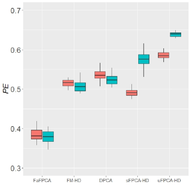
(a) $K=10,$ ${\bf\Sigma}={\bf I}$(red), ${\bf\Sigma}\neq{\bf I}$(blue)

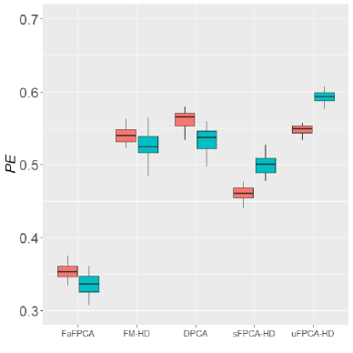
(b) $K=2,$ ${\bf\Sigma}={\bf I}$(red), ${\bf\Sigma}\neq{\bf I}$(blue)

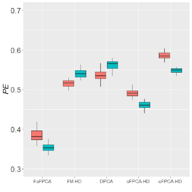
(c) ${\bf\Sigma}={\bf I},$ $K=10$(red) and $K=2$(blue)

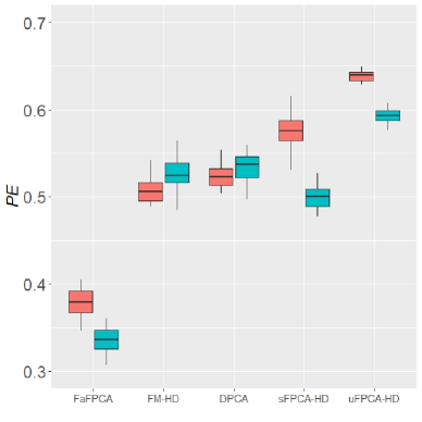
(d) ${\bf\Sigma}\neq{\bf I},$ $K=10$(red) and $K=2$(blue)

Figure 1: The PEs of the FaFPCA, FM-HD, DPCA, sFPCA-HD and uPFCA-HD methods under the cases listed in Scenario 1.

We carried out the computation on a single 4-core personal laptop with 16 GB of RAM. Table 1 shows the average running time of 200 repetitions for Case I with $K=2$. Table 1 shows that the proposed FaFPCA approach is much faster than the other methods except FM-HD, which only considers model (1) and does not estimate eigenfunctions and factor scores. uFPCA-HD requires an extremely large amount of time because uFPCA is applied to each of the $p$ curves separately.

Table 1: The computational time in seconds of the five methods.

	FaFPCA	FM-HD	DPCA	sFPCA-HD	uFPCA-HD
Mean	0.0300	0.0190	0.4570	0.2430	77.3500
SD	0.0097	0.0095	0.0178	0.0283	3.0647

Scenario 2: Figure 2 displays RMSE_l for loadings, RMSE_f for factors and RMSE_e for eigenfunctions using the proposed FaFPCA method for Scenario 2 with $(q,K)=(5,2)$ when $(n,p)$ varies. The results in Figure 2 indicate that the precision of ${\bf B},\bm{\zeta}$ and ${\bm{\Phi}}(t)$ increases as $n$ or $p$ increases, which is consistent with the theoretical results. In particular, the precision of $\bm{\zeta}$ is more sensitive to $p$ than to $n$, while that of ${\bf B}$ is more sensitive to $n$. This is because the estimator for $\bm{\zeta}_{i}$ is based on $p$ functions of individual $i$; however, the estimator for ${\bf B}$ is mainly based on $n$ individuals.

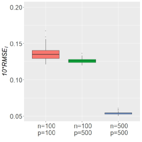
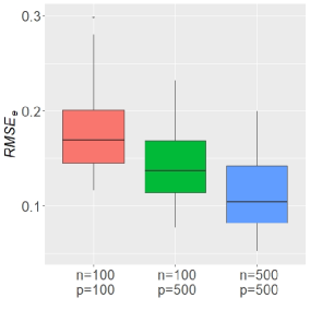
Figure 2: The boxplots of $10\times$RMSE_l,RMSE_f and RMSE_e (from left to right) of the FaFPCA for Scenario 2 with $n,p=100,500$. The RMSE_l, RMSE_f and RMSE_e are the root of mean square errors for loadings, factors and eigenfunctions, respectively.

To show the effect of the number of observations, we take $n_{i}$ from 5 to 50 given $n=p=100$ and $(q,K)=(5,2)$. The results in Figure 3 show that the estimators are quite stable with respect to $n_{i}$ except for small $n_{i}$ values. When $n_{i}$ is small, the matrix $\sum_{l=1}^{n_{i}}{\bf M}(t_{il}){\bf M}^{\prime}(t_{il})$ in ${\bf w}_{ik}$ might be irreversible. To avoid this problem, we add a term $\lambda{\bf I}_{\tau_{n}}$, where $\lambda$ is small, to $\sum_{l=1}^{n_{i}}{\bf M}(t_{il}){\bf M}^{\prime}(t_{il})$ to ensure invertibility. This may cause extra bias for the estimations of factors and eigenfunctions when $n_{i}$ is small. From Figure 3, we also observe an interesting phenomenon as $n_{i}$ increases, RMSE_l for loadings increases, while RMSE_f and RMSE_e for factors and eigenfunctions, respectively, decrease. This can be attributed the following two aspects. On the one hand, the loadings are estimated mainly based on $n$ samples, rather than $n_{i}$ or $p$; hence, the increasing $n_{i}$ values may introduce extra noise due to the integration of all observations using (6). On the other hand, the factors $\bm{\zeta}_{i}$ are estimated mainly based on the observations from individual $i$; hence, the estimation of the factors becomes better as $n_{i}$ increases, although becomes stable when $n_{i}$ is large enough, for example, when $n_{i}>10$ in the cases. The estimation of eigenfunctions has a similar performance as that of the factors since they are simultaneously estimated.

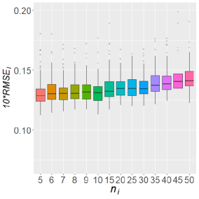
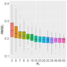
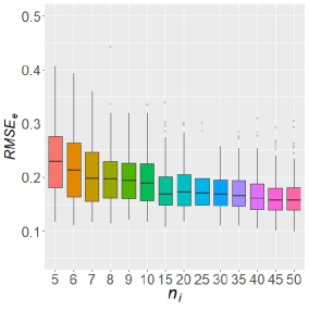
Figure 3: The boxplots of $10\times$RMSE_l, RMSE_f and RMSE_e (from left to right) of the FaFPCA when $n_{i}$ changes from 5 to 50. The RMSE_l, RMSE_f and RMSE_e are the root of mean square errors for loadings, factors and eigenfunctions, respectively.

5 Real Data Analysis

Alzheimer’s disease (AD) is irreversible and the most common form of dementia, and it can result in the loss of thinking, memory and language skills. It is important to determine the progress of AD by monitoring alterations in the brain and to detect the disease at an early stage. Particularly, it is well known that the atrophy of the region of interest (ROI) is associated with AD detection and some studies consider local brain volumes for characterizing regional atrophy (Zhao et al.,, 2019; Zhong et al.,, 2021; Li et al.,, 2022). In the paper, we use the brain volume density values within different ROIs to detect the progression of AD. The dataset includes a subset of participants with 766 subjects enrolled in the first phase of the ADNI study (Mueller et al.,, 2005) with AD, mild cognitive impairment (MCI, an early stage of AD) and cognitively normal (CN). A total of 172, 378 and 216 participants were diagnosed with AD, MCI and CN, respectively. Each participant’s record consists of the brain volume density values of 90 ROIs for each of the 501 equispaced sampling volumes in the interval of $[-255,\ 255]$, so that we can regard the brain volume density as a curve. To be specific, we denote ${\bf X}_{i}(t)$ by the brain volume density curves of ROIs of the $i$-th individual, which are functions of the log of the Jacobian volume (denoted by $t$). We scale the log Jacobian volume into $[0,\ 1]$ before analysis and the summary of the ROIs is shown in Table 2. Consequently, 90 ROIs are high-dimensional functional variables that can be analyzed by the proposed FaFPCA approach, as well as the methods mentioned in Section 4 for comparison.

We apply FaFPCA, FM-HD, DPCA, sFPCA-HD and uFPCA-HD to the data without the label information of AD, MCI and CN. First, based on the criteria in Section 2.3, we choose $q=5$ factors and $K=3$ eigenfunctions for FaFPCA. Similarly, on the grounds of the proportion of variability, we choose $q=5$, $K=15$, $K=33$ and $K=2$ for the FM-HD, DPCA, sFPCA-HD and uFPCA-HD methods, respectively. We randomly set 60% of the dataset as the training set and the other data as the test set with 200 repeats. Figure 4(a) presents the PEs of FaFPCA, FM-HD, DPCA, sFPCA-HD and uFPCA-HD with the corresponding selected hyperparameters and shows that FaFPCA yeilds the estimator with the highest prediction accuracy. In addition, Figure 4(a) also shows that the sFPCA-HD and uFPCA-HD methods are the worst in terms of PE, which indicates that the correlation among functional variables might be strong in the ADNI data.

(a)

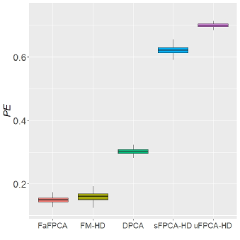
(b)

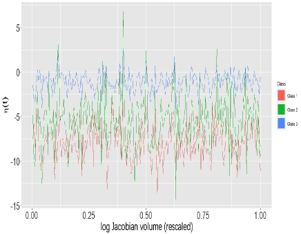
Figure 4: (a) The PEs of FaFPCA, FM-HD, DPCA, sFPCA-HD and uFPCA-HD for the ADNI dataset. (b) The regression coefficient functions of choosed ROIs in each class.

Now, we investigate details about the factors in Figure 5. Based on the top ten largest absolute values of the loadings, factor 1 extracts the feature mainly from variables ROI₁₂, ROI₁₅, ROI₁₆, ROI₅₁, ROI₉₁, ROI₉₂, ROI₆₃₁, ROI₆₃₂, ROI₁₀₁₆ and ROI₂₀₁₆, which represent the information on the brain regions starting from the forebrain, arriving at the base of the brain, and then returning to the afterbrain. These ROIs exist in the bottom lateral part of the brain and mostly in the cerebellum. Factor 2 withdraws the information of variables ROI₅, ROI₁₆, ROI₁₇, ROI₁₈, ROI₂₈, ROI₅₀, ROI₅₃, ROI₅₄, ROI₄₉ and ROI₆₀, which express information on the basal nucleus and are located deeply in the white matter of the brain. Factors 3-5 extract the information from regions similar to those of factor 2.

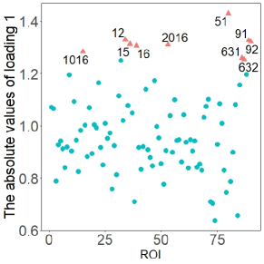
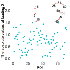
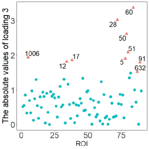
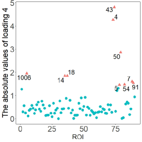
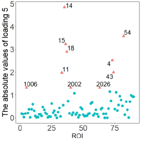
Figure 5: The absolute values of the 5 loadings, where the red triangular dots are the first 10 largest absolute values of loadings.

Since $q=5$ is selected, we can use the 5-dimensional vector to represent each ROI, resulting in $\widehat{\bf B}\in\mathbb{R}^{90\times 5}$ for 90 ROIs. Then, based on the estimated $\widehat{\bf B}$, we cluster the ROIs into 3 classes by $K$-means, and the clusters are displayed in Table 2. We can see that class 1 mainly includes the ROIs in the basal nucleus, class 2 mainly contains the ROIs in the junction between the brain and basal nucleus, and class 3 involves the ROIs in the brain, including the lateral and medial parts of the left and right hemispheres.

Table 2: The ROIs and their clusters.

ROI	name	ROI	name	ROI	name
Class 1
5	left inferior lateral ventricle	18	left amygdala	91	left basal forebrain
10	left thalamus proper	24	CSF	92	right basal forebrain
11	left caudate	28	left ventral DC	632	cerebellar vermal lobules
12	left putamen	49	right thalamus proper		VIII-X
14	3rd ventricle	50	right caudate	1014	left medial orbitofrontal
15	4th ventricle	53	right hippocampus	1026	left rostral anterior
16	Brain stem	54	right amygdala		cingulate
17	left hippocampus	60	right ventral DC	2002	right caudal anterior
2012	right lateral orbitofrontal	2014	right medial orbitofronta		cingulate
2023	right posterior cingulate
Class 2
51	right putamen	1016	left parahippocampal	1025	left precuneus
630	cerebellar vermal lobules I-V	1017	left paracentral	1035	left insula
631	cerebellar vermal lobules VI-VII	1021	left pericalcarine	2013	right lingual
1012	left lateral orbitofrontal	1023	left posterior cingulate	2017	right paracentral
1013	left lingual	1024	left precentral	2021	right pericalcarine
2025	right precuneus	2026	right rostral anterior cingulate
Class 3
4	left lateral ventricle	1018	left pars opercularis	2010	right isthmus cingulate
6	left cerebellum exterior	1019	left pars orbitalis	2011	right lateral occipital
7	left cerebellum white matter	1020	left pars triangularis	2015	right mid-temporal
43	right lateral ventricle	1022	left postcentral	2016	right parahippocampal
45	right cerebellum exterior	1027	left rostral mid-frontal	2018	right pars opercularis
46	right cerebellum white matter	1028	left superior frontal	2019	right pars orbitalis
1002	left caudal anterior cingulate	1029	left superior parietal	2020	right pars triangularis
1003	left caudal mid-frontal	1030	left superior temporal	2022	right postcentral
1005	left cuneus	1031	left supramarginal	2024	right precentral
1006	left entorhinal	1034	left transverse temporal	2027	right rostral mid-frontal
1007	left fusiform	2003	right caudal mid- frontal	2028	right superior frontal
1008	left inferior parietal	2005	right cuneus	2029	right superior parietal
1009	left inferior temporal	2006	right entorhinal	2030	right superior temporal
1010	left isthmus cingulate	2007	right fusiform	2031	right supramarginal
1011	left lateral occipital	2008	right inferior parietal	2034	right transverse temporal
1015	left mid-temporal	2009	right inferior temporal	2035	right insula

We also investigate the effects of the ROIs on AD. First, we conduct multivariate logistic regression with AD, MCI and CN as responses and $\widehat{\bm{\zeta}}_{i}$ as covariates. The regression coefficients are denoted by $\bm{\alpha}$. Hence, $\bm{\alpha}^{\prime}\widehat{\bm{\zeta}}_{i}$ can be regarded as the measurement of the effect of the ROIs on AD. On the other hand, by multiplying $p^{-1}{\bm{\Phi}}(t){\bf B}^{\prime}$ on both sides of (4) and coupling it with the identification condition $p^{-1}{\bf B}^{\prime}{\bf B}={\bf I}_{q}$, we obtain $p^{-1}{\bm{\Phi}}(t){\bf B}^{\prime}{\bf X}_{i}(t)\approx{\bm{\Phi}}(t){\bm{\Phi}}^{\prime}(t)\bm{\zeta}_{i}.$ After combining it with the identification condition $\int{\bm{\Phi}}(t){\bm{\Phi}}(t)^{\prime}dt={\bf I}$, we have

$$p^{-1}\int\bm{\alpha}^{\prime}{\bm{\Phi}}(t){\bf B}^{\prime}{\bf X}_{i}(t)dt\approx\bm{\alpha}^{\prime}\int{\bm{\Phi}}(t){\bm{\Phi}}^{\prime}(t)dt\bm{\zeta}_{i}=\bm{\alpha}^{\prime}\bm{\zeta}_{i}.$$

Then, the regression relationship $\bm{\alpha}^{\prime}\bm{\zeta}_{i}$ between response $Y_{i}$ and factor $\bm{\zeta}_{i}$ can be written as $\int\bm{\eta}^{\prime}(t){\bf X}_{i}(t)dt$ between $Y_{i}$ and original functional covariates ${\bf X}_{i}(t)$, where $\bm{\eta}(t)=(\eta_{1}(t),\cdots,\eta_{p}(t))^{\prime}=p^{-1}{\bf B}{\bm{\Phi}}^{\prime}(t)\bm{\alpha}$ is the regression coefficient function. To visualize the coefficient function, we choose one ROI from each class in Table 2 and plot the corresponding estimated coefficient function $\widehat{\eta}_{j}(t)$ for $\eta_{j}(t)$ in Figure 4(b), which shows that the estimated coefficient function $\widehat{\bm{\eta}}(t)$ fluctuates violently around a horizontal line. This inspires us to compute the cumulative term ${\bm{\beta}}=\int\widehat{\bm{\eta}}(t)dt$ to measure the effects of the ROIs on the response. Furthermore, for each ROI $j$, we perform hypothesis testing $\beta_{j}=0$ based on 200 bootstrap samples to test the effect of ROI $j$ on AD. As a result, we identify 41 significant ROIs, as displayed in Table 3. All the significant ROI effects are negative, which implies that brain atrophy is associated with AD and is consistent with previous studies (Double et al.,, 1996). For example, the following conclusions have been found for the 41 significant ROIs:

• Medial temporal lobe (ROI₂₀₁₅) atrophy was reported by Fruijtier et al., (2019) to be one of the three best validated neuroimaging biomarkers for AD.

• The tau protein is an indicator of the extent of neuronal damage, and its pathology was verified by Solders et al., (2022) to propagate in a prion-like manner along the LC-transentorhinal cortex (ROI₁₀₀₆ and ROI₂₀₀₆) and white matter (ROI₄₆) pathway.

• In addition, frontal lobe (ROI₁₀₀₃, ROI₁₀₂₈,ROI₂₀₀₃ and ROI₂₀₂₇) atrophy is a prominent symbol of AD and can accelerate the lesions of AD. This was reported by Simona et al., (2016).

• The atrophy of the parietal lobe (ROI₁₀₀₈ and ROI₁₀₂₉), insula (ROI₂₀₃₅) and hippocampus (ROI₁₇ and ROI₅₃) was found to induce AD by Foundas et al., (1997). Moreover, from Table 3, we can see that the effect of the left hippocampus (ROI₁₇) is larger than that of the right hippocampus (ROI₅₃), which is consistent with the findings of Philip et al., (2021), which state that the atrophy of left hippocampus is more severe than that of the right hippocampus in AD patients.

• The predictive function of fusiform gyrus (ROI₁₀₀₇) atrophy at the early stage of AD has been reported by Chang et al., (2016). Donovan et al., (2014) indicated damage to the supramarginal gyrus (ROI₁₀₃₁) atrophy to the human visual system in AD patients.

• The associations of atrophy in the caudate nucleus (ROI₅₀), pars triangularis (ROI₁₀₂₀ and ROI₂₀₂₀), pars opercularis (ROI₁₀₁₈ and ROI₂₀₁₈), and amygdala (ROI₅₄) with AD have also been extensively reported in the literature, for example, Pearce et al., (1984); Whitwell, (2010) and Stéphane et al., (2011).

Table 3: Estimates, SDs and $p$ values of ${\bm{\beta}}=\int\bm{\eta}(t)dt$ for the ADNI data, where $\bm{\eta}(t)$ is the regression coefficient function of the ROIs.

ROI	Estimate	SD	$p$ value	ROI	Estimate	SD	$p$ value	ROI	Estimate	SD	$p$ value
5	-5.9829	1.9892	0.0026	1008	-1.7920	0.6487	0.0057	2008	-2.7590	0.7487	0.0002
14	-4.0130	1.8183	0.0273	1009	-3.8436	0.9955	0.0001	2009	-4.8168	1.2551	0.0001
17	-6.0605	1.6149	0.0002	1011	-2.9302	0.8575	0.0006	2010	-2.3420	0.8745	0.0074
28	-9.3520	2.4988	0.0002	1018	-3.4751	1.0386	0.0008	2015	-3.1155	0.8163	0.0001
45	-2.5556	0.7636	0.0008	1020	-3.6396	0.9609	0.0002	2018	-2.4459	0.7143	0.0006
46	-3.1817	1.2945	0.0140	1028	-1.6740	0.6912	0.0154	2019	-1.7958	0.7866	0.0224
50	-7.4244	3.1591	0.0188	1029	-3.1541	0.8261	0.0001	2020	-1.8009	0.6835	0.0084
53	-4.9068	1.2157	0.0001	1030	-4.1952	1.0764	0.0001	2022	-1.2041	0.6140	0.0499
54	-5.9669	1.7803	0.0008	1031	-2.3494	0.6523	0.0003	2027	-1.6122	0.6545	0.0138
60	-10.1306	2.8457	0.0004	1034	-3.1273	1.0865	0.0004	2030	-3.2471	0.8374	0.0001
1003	-3.4179	0.9363	0.0003	2003	-2.6540	0.7662	0.0005	2031	-2.7265	0.7388	0.0002
1005	-1.8912	0.6732	0.0049	2005	-1.7878	0.6582	0.0066	2034	-2.0218	0.9236	0.0286
1006	-6.9455	2.1871	0.0015	2006	-2.8513	0.8757	0.0011	2035	-1.7238	0.7776	0.0266
1007	-2.9910	0.7921	0.0002	2007	-3.1506	0.8217	0.0001

6 Discussion

In this paper, we propose FaFPCA to extract features from high-dimensional functional data. By building some moment equations, we estimate loadings, scores and eigenfunctions in closed form without rotation. We also establish the theoretical properties of the proposed estimator, including the convergence rate and asymptotic normality. The proposed FaFPCA approach has the following advantages. (1) Computational efficiency. With the proper rewriting of the FaFPCA model, we directly estimate loadings, scores and eigenfunctions in closed form so that complicated and likely nonconvergent iterations can be avoided. (2) Blessing of dimensionality. In high-dimensional FDA, the dimension of function $p$ is a burden for estimation and inference. In contrast, FaFPCA provides functional principal analysis under the framework of a factor model; as a result, the dimensionality curse becomes dimensionality welfare, which is confirmed by Theorems 1-4 and simulation studies. (3) Theoretical interpretability. We give the theoretical properties of FaFPCA and show the relation to the traditional high-dimensional factor model. (4) High prediction accuracy. Since we use both the correlation among the high-dimensional functional variables and the dependence over time, the proposed FaFPCA approach has a higher prediction accuracy than the existing methods, which is confirmed by real data analysis and simulation studies.

Various extensions can be considered in the future. For example, we can extend linear FaFPCA to the generalized case for discrete functional data. However, the computational and the theoretical availability for a nonlinear framework are worthy of further investigation. In practice, the observations ${\bf X}_{i}(t),i=1,\cdots,n$ may be serially dependent, such as those considered by Tavakoli et al., (2021) and Guo et al., (2022), it is interesting to extend FaFPCA to high-dimensional functional time series analysis. In addition, in the paper, we only consider the dimension reduction of high-dimensional functional data. The features captured by the factors are the most important directions concerning the information of high-dimensional functional covariates alone rather than under the supervision of the response. It is an important question on how to extract factors from high-dimensional functional covariates in the direction supervised by a response variable.

References

- Ash and Gardner, (1975) Ash, R. and Gardner, M. (1975). Topics in stochastic processes. Academic Press.
- Bai, (2003) Bai, J. (2003). Inferential theory for factor models of large dimensions. Econometrica, 71(1):135–171.
- Bai and Liao, (2013) Bai, J. and Liao, Y. (2013). Statistical inferences using large estimated covariances for panel data and factor models. arXiv:1307.2662.
- Bai and Ng, (2002) Bai, J. and Ng, S. (2002). Determining the number of factors in approximate factor models. Econometrica, 70(1):191–221.
- Bai and Ng, (2006) Bai, J. and Ng, S. (2006). Confidence intervals for diffusion index forecasts and inference for factor-augmented regressions. Econometrica, 74(4):1133–1150.
- Bai and Ng, (2013) Bai, J. and Ng, S. (2013). Principal components estimation and identification of static factors. Journal of Econometrics, 176(1):18–29.
- Chang et al., (2020) Chang, J., Chen, C., Qiao, X., and Yao, Q. (2020). An autocovariance-based learning framework for high-dimensional functional time series. arXiv:2008.12885.
- Chang et al., (2016) Chang, Y. T., Huang, C. W., Chen, N. C., Lin, K. J., Huang, S. H., Chang, W. N., Shih-Wei, H., Che-Wei, H., Chen, H. H., and Chang, C. C. (2016). Hippocampal amyloid burden with downstream fusiform gyrus atrophy correlate with face matching task scores in early stage alzheimer’s disease. Frontiers in Aging Neuroence, 8.
- Chiou et al., (2014) Chiou, J.-M., Chen, Y.-T., and Yang, Y.-F. (2014). Multivariate functional principal component analysis: A normalization approach. Statistica Sinica, 24(4):1571–1596.
- Chiou and Müller, (2014) Chiou, J.-M. and Müller, H.-G. (2014). Linear manifold modelling of multivariate functional data. Journal of the Royal Statistical Society: Series B (Statistical Methodology), 76(3):605–626.
- Donovan et al., (2014) Donovan, N. J., Wadsworth, L. P., Lorius, N., Locascio, J. J., Rentz, D. M., Johnson, K. A., Sperling, R. A., and Marshall, G. A. (2014). Regional cortical thinning predicts worsening apathy and hallucinations across the alzheimer disease spectrum. American Journal of Geriatric Psychiatry, 22(11):1168–1179.
- Double et al., (1996) Double, K., Halliday, G., Krill, J., Harasty, J., Cullen, K., Brooks, W., Creasey, H., and Broe, G. (1996). Topography of brain atrophy during normal aging and alzheimer’s disease. Neurobiology of Aging, 17(4):513–521.
- Fan et al., (2013) Fan, J., Liao, Y., and Mincheva, M. (2013). Large covariance estimation by thresholding principal orthogonal complements. Journal of the Royal Statistical Society: Series B (Statistical Methodology), 75(4):603–680.
- Fang et al., (2021) Fang, Q., Guo, S., and Qiao, X. (2021). Finite sample theory for high-dimensional functional/scalar time series with applications. arXiv:2004.07781.
- Ferraty and Vieu, (2006) Ferraty, F. and Vieu, P. (2006). Nonparametric functional data analysis. Springer.
- Foundas et al., (1997) Foundas, A. L., Leonard, C. M., Mahoney, S. M., Agee, O. F., and Heilman, K. M. (1997). Atrophy of the hippocampus, parietal cortex, and insula in alzheimer’s disease: A volumetric magnetic resonance imaging study. Cognitive and Behavioral Neurology, 10(2):81–89.
- Fruijtier et al., (2019) Fruijtier, A. D., Visser, L., Maurik, I., Zwan, M., and Smets, E. (2019). Abide delphi study: topics to discuss in diagnostic consultations in memory clinics. Alzheimer’s Research and Therapy, 11(1):77.
- Gao et al., (2019) Gao, Y., Shang, H. L., and Yang, Y. (2019). High-dimensional functional time series forecasting: An application to age-specific mortality rates. Journal of Multivariate Analysis, 170:232–243.
- Górecki et al., (2018) Górecki, T., Krzyśko, M., Waszak, L., and Wołyński, W. (2018). Selected statistical methods of data analysis for multivariate functional data. Statistical Papers, 59(1):153–182.
- Grith et al., (2018) Grith, M., Wagner, H., Härdle, W. K., and Kneip, A. (2018). Functional principal component analysis for derivatives of multivariate curves. Statistica Sinica, 28(4):2469–2496.
- Guo and Qiao, (2020) Guo, S. and Qiao, X. (2020). On consistency and sparsity for high-dimensional functional time series with application to autoregressions. arXiv:2003.11462.
- Guo et al., (2022) Guo, S., Qiao, X., and Wang, Q. (2022). Factor modelling for high-dimensional functional time series. arXiv:2112.13651.
- Hall and Hosseini-Nasab, (2006) Hall, P. and Hosseini-Nasab, M. (2006). On properties of functional principal components analysis. Journal of the Royal Statistical Society: Series B (Statistical Methodology), 68(1):109–126.
- Hall et al., (2008) Hall, P., Müller, H., and Yao, F. (2008). Modelling sparse generalized longitudinal observations with latent gaussian processes. Journal of the Royal Statistical Society: Series B (Statistical Methodology), 70(4):703–723.
- Han et al., (2018) Han, K., Müller, H.-G., and Park, B. U. (2018). Smooth backfitting for additive modeling with small errors-in-variables, with an application to additive functional regression for multiple predictor functions. Bernoulli, 24(2):1233–1265.
- Happ and Greven, (2018) Happ, C. and Greven, S. (2018). Multivariate functional principal component analysis for data observed on different (dimensional) domains. Journal of the American Statistical Association, 113(522):649–659.
- Happ et al., (2019) Happ, C., Scheipl, F., Gabriel, A.-A., and Greven, S. (2019). A general framework for multivariate functional principal component analysis of amplitude and phase variation. Statistical Papers, 8(e220):1–12.
- Horváth and Kokoszka, (2012) Horváth, L. and Kokoszka, P. (2012). Inference for Functional Data with Applications. Springer Science & Business Media.
- Hsing and Eubank, (2015) Hsing, T. and Eubank, R. (2015). Theoretical Foundations of Functional Data Analysis, with an Introduction to Linear Operators. John Wiley & Sons.
- Hu and Yao, (2021) Hu, X. and Yao, F. (2021). Dynamic principal subspaces in high dimensions. arXiv:2104.03087.
- Hu and Yao, (2022) Hu, X. and Yao, F. (2022). Sparse functional principal component analysis in high dimensions. Statistica Sinica, 38:1–22.
- Jacques and Preda, (2014) Jacques, J. and Preda, C. (2014). Model-based clustering for multivariate functional data. Computational Statistics and Data Analysis, 71:92–106.
- James et al., (2000) James, G. M., Hastie, T. J., and Sugar, C. A. (2000). Principal component models for sparse functional data. Biometrika, 87(3):587–602.
- Jiang et al., (2019) Jiang, F., Ma, Y., and Wei, Y. (2019). Sufficient direction factor model and its application to gene expression quantitative trait loci discovery. Biometrika, 106(2):417–432.
- Kokoszka and Reimherr, (2017) Kokoszka, P. and Reimherr, M. (2017). Introduction to Functional Data Analysis. CRC Press.
- Kong et al., (2016) Kong, D., Xue, K., Yao, F., and Zhang, H. (2016). Partially functional linear regression in high dimensions. Biometrika, 103(1):147–159.
- Li et al., (2018) Li, Q., Cheng, G., Fan, J., and Wang, Y. (2018). Embracing the blessing of dimensionality in factor models. Journal of the American Statistical Association, 113(521):380–389.
- Li et al., (2022) Li, T., Zhu, H., Li, T., and Zhu, H. (2022). Asynchronous functional linear regression models for longitudinal data in reproducing kernel hilbert space. Biometrics, pages 1–16. https://doi.org/10.1111/biom.13767.
- Li and Hsing, (2010) Li, Y. and Hsing (2010). Deciding the dimension of effective dimension reduction space for functional and high-dimensional data. The Annals of Statistics, 38(5):3028–3062.
- Lian, (2013) Lian, H. (2013). Shrinkage estimation and selection for multiple functional regression. Statistica Sinica, 23(1):51–74.
- Lin et al., (2018) Lin, Z., Müller, H. G., and Yao, F. (2018). Mixture inner product spaces and their application to functional data analysis. The Annals of Statistics, 46(1):370–400.
- Liu et al., (2022) Liu, W., Lin, H., Zheng, S., and Liu, J. (2022+). Generalized factor model for ultra-high dimensional correlated variables with mixed types. Journal of the American Statistical Association, online.
- Mueller et al., (2005) Mueller, S. G., Weiner, M. W., Thal, L. J., Petersen, R. C., Jack, C., Jagust, W., Trojanowski, J. Q., Toga, A. W., and Beckett, L. (2005). Alzheimer’s disease neuroimaging initiative. Neuroimaging clinics of North America, 15(4):869–877.
- Panaretos et al., (2010) Panaretos, V. M., Kraus, D., and Maddocks, J. H. (2010). Second-order comparison of gaussian random functions and the geometry of dna minicircles. Journal of the American Statistical Association, 105(490):670–682.
- Pearce et al., (1984) Pearce, B. R., Palmer, A. M., Bowen, D. M., Wilcock, G. K., and Davison, A. N. (1984). Neurotransmitter dysfunction and atrophy of the caudate nucleus in alzheimer’s disease. Neurochemical Pathology, 2(4):221–232.
- Philip et al., (2021) Philip, S., Bart, D. S., Miia, K., Henne, H., Gael, C., Charlotte, E. T., Jeffrey, C., and Wiesje, M. v. d. F. (2021). Alzheimer’s disease. Cognitive and Behavioral Neurology, 397:1577–1590.
- Ramsay, (1982) Ramsay, J. O. (1982). When the data are functions. Psychometrika, 47(4):379–396.
- Ramsay and Silverman, (2002) Ramsay, J. O. and Silverman, B. W. (2002). Applied Functional Data Analysis. Springer.
- Ramsay and Silverman, (2005) Ramsay, J. O. and Silverman, B. W. (2005). Functional Data Analysis. Springer.
- Rice and Silverman, (1991) Rice, J. A. and Silverman, B. W. (1991). Estimating the mean and covariance structure nonparametrically when the data are curves. Journal of the Royal Statistical Society: Series B (Statistical Methodological), 53(1):233–243.
- Simona et al., (2016) Simona, S., Philip, S. I., Susanne, M., Duygu, T., Niklas, M., Clifford, R., Charles, D., Ronald, P., Paul, S. A., Weiner, M. W., ScottMackin, R., and Initiative, A. D. N. (2016). Chronic depressive symptomatology in mild cognitive impairment is associated with frontal atrophy rate which hastens conversion to alzheimer dementia. American Journal of Geriatric Psychiatry, 24(2):126–135.
- Solders et al., (2022) Solders, S. K., Galinsky, V. L., Clark, A. L., Sorg, S. F., Weigand, A. J., Bondi, M. W., and Frank, L. R. (2022). Diffusion mri tractography of the locus coeruleus-transentorhinal cortex connections using go-esp. Magnetic Resonance in Medicine, 87:1816–1831.
- Solea and Dette, (2021) Solea, E. and Dette, H. (2021). Nonparametric and high-dimensional functional graphical models. arXiv:2103.10568.
- Stone, (1980) Stone, C. J. (1980). Optimal rates of convergence for nonparametric estimators. The Annals of Statistics, 8(6):1348–1360.
- Stéphane et al., (2011) Stéphane, P. P., Dautoff, R., Morris, J. C., Barrett, L. F., and Dickerson, B. C. (2011). Amygdala atrophy is prominent in early alzheimer’s disease and relates to symptom severity. Psychiatry Research, 194(1):7–13.
- Tang et al., (2021) Tang, C., Shang, H. L., and Yang, Y. (2021). Multi-population mortality forecasting using high-dimensional functional factor models. arXiv:2109.04146.
- Tang and Shi, (2021) Tang, C. and Shi, Y. (2021). Forecasting high-dimensional financial functional time series: An application to constituent stocks in dow jones index. Journal of Risk and Financial Management, 14(8):343.
- Tavakoli et al., (2021) Tavakoli, S., Nisol, G., and Hallin, M. (2021). High-dimensional functional factor models. arXiv:1905.10325.
- Whitwell, (2010) Whitwell, J. L. (2010). Progression of atrophy in alzheimer’s disease and related disorders. Neurotoxicity Research, 18(3-4):339–346.
- Wong et al., (2019) Wong, R. K. W., Li, Y., and Zhu, Z. (2019). Partially linear functional additive models for multivariate functional data. Journal of the American Statistical Association, 114(525):406–418.
- Yao et al., (2005) Yao, F., Müller, H.-G., and Wang, J.-L. (2005). Functional data analysis for sparse longitudinal data. Journal of the American Statistical Association, 100(470):577–590.
- Zhao et al., (2019) Zhao, B., Ibrahim, J. G., Li, Y., Li, T., Wang, Y., Shan, Y., Zhu, Z., Zhou, F., Zhang, J., Huang, C., Liao, H., Yang, L., Thompson, P. M., and Zhu, H. (2019). Heritability of regional brain volumes in large-scale neuroimaging and genetic studies. Cerebral Cortex, 29(7):2904–2914.
- Zhong et al., (2021) Zhong, Q., Lin, H., and Li, Y. (2021). Cluster non-gaussian functional data. Biometrics, 77(3):852–865.
- Zhou et al., (2018) Zhou, L., Lin, H., and Liang, H. (2018). Efficient estimation of the nonparametric mean and covariance functions for longitudinal and sparse functional data. Journal of the American statistical association, 113(524):1550–1564.
- Zhu et al., (2016) Zhu, H., Strawn, N., and Dunson, D. B. (2016). Bayesian graphical models for multivariate functional data. The Journal of Machine Learning Research, 17(1):7157–7183.