:
\theoremsep
Explainability of Traditional and Deep Learning Models on Longitudinal Healthcare Records
Abstract
Recent advances in deep learning have led to interest in training deep learning models on longitudinal healthcare records to predict a range of medical events, with models demonstrating high predictive performance. Predictive performance is necessary but insufficient, however, with explanations and reasoning from models required to convince clinicians for sustained use. Rigorous evaluation of explainability is often missing, as comparisons between models (traditional versus deep) and various explainability methods have not been well-studied. Furthermore, ground truths needed to evaluate explainability can be highly subjective depending on the clinician’s perspective. Our work is one of the first to evaluate explainability performance between and within traditional (XGBoost) and deep learning (LSTM with Attention) models on both a global and individual per-prediction level on longitudinal healthcare data. We compared explainability using three popular methods: 1) SHapley Additive exPlanations (SHAP), 2) Layer-Wise Relevance Propagation (LRP), and 3) Attention. These implementations were applied on synthetically generated datasets with designed ground-truths and a real-world medicare claims dataset. We showed that overall, LSTMs with SHAP or LRP provides superior explainability compared to XGBoost on both the global and local level, while LSTM with dot-product attention failed to produce reasonable ones. With the explosion of the volume of healthcare data and deep learning progress, the need to evaluate explainability will be pivotal towards successful adoption of deep learning models in healthcare settings.
1 Introduction
Longitudinal healthcare records are defined as sets of health information generated temporally by one or more encounters in a care setting. As the digitization of longitudinal healthcare records data continues, traditional modeling techniques are increasingly challenged in understanding the high-dimensional complexity and non-linear nature of medical data. Deep learning models, especially those originating from natural language processsing (NLP) field, have found predictive success when applied to longitudinal healthcare data. These models are capable of leveraging time-dependent and complex data beyond typical human capabilities, as shown by Meyer et al. (2018) on raw ICU data with sequence models.
Success in prediction performance is necessary but insufficient for adoption of AI-based models by the healthcare community. Tonekaboni et al. (2019) showed that high level of transparency from a ML-based system is necessary for sustained use in clinical settings, and remains a significant barrier. Norrie (2018) highlighted this transparency difficulty on Meyer et al. (2018)’s work , ‘unlike models such as the simple logistic prediction model … deep learning rests upon hidden factors that uncover complex, high-order data patterns; by definition, we do not know — and far less are able to describe or explain — what such a model is doing.’ Recent healthcare applications of deep learning continue to focus on predictive performance metrics such as area under curve (AUC), with model explainability receiving qualitative treatment. Examples include Rajkomar et al. (2018) on predicting readmissions, mortality and length of stay with LSTMs with a single example of interpretability. Zhang et al. (2018) qualitatively described attention-based LSTM model interpretation of two different patient cases for all-cause hospitalization. Rasmy et al. (2020) similarly notes medical concept patterns learned by a BERT-based model. Consequently, traditional ML methods continue to be used, including Bos et al. (2018) and Ross et al. (2019).
It is thus of clinical relevance and importance that more studies are conducted by healthcare-focused ML practitioners into understanding model behavior. It is also currently unclear how explainability derived from more traditional approaches compare with quantitative explainability or interpretability derived from deep learning methods when applied to longitudinal healthcare data. This lack of quantitative focus on healthcare model explainability and lack of comparisons between traditional ML and deep learning based approaches is primarily due the varied approaches and expectations surrounding this topic. There is currently little consensus within the ML community, including healthcare-focused ML researchers, on the definition of interpretability and explainability. Some practitioners, including us in this work, have chosen to use both terms interchangeably, while others including Rudin (2019) draw distinctions between the two. Secondly, there is also the type of interpretability/explainability: global interpretability seeks to explain overall model behavior; local interpretability seeks to explain at the per prediction level (Stiglic et al. (2020)). Thirdly, there is the distinction of model-agnostic versus model-specific type of explainability. Model-agnostic approaches, including SHAP treat an already-trained model as a black box while providing interpretations. Lundberg et al. (2019) utilized SHAP to provide visual interpretations for a tree-based model on the epidemiological data and for hypoxaemia during surgery (Lundberg et al. (2018)).
Distinct from model-agnostic approaches, model-specific approaches require understanding of the underlying model architecture. This includes Layer-wise Relevance Propagation (LRP), a general method for explaining deep learning models originally proposed by Bach et al. (2015). LRP provides explainability by backwards-attributing prediction scores through the network back to the input space. Other NLP researchers provide explainability via inclusion of attention mechanisms within the model architecture. The extracted attention scores is thought to provide insight into a deep learning model’s mechanisms, with inputs or time-steps (for sequence models) with high attention scores believed to be of higher importance. This has very recently been called into question and is area of active debate, as evidenced by Jain and Wallace (2019)’s work titled ‘Attention is not Explanation’ and a responding paper by Wiegreffe and Pinter (2019) titled ‘Attention is not not Explanation’.
Finally, the type of healthcare data studied heavily determines ML model and explainability. On the simpler end, traditional methods can provide accurate and explainable predictions with a curated set of well-understood predictors. On the other extreme, temporally organized datasets such as electronic health records (EHR) and claims datasets allow for complex deep learning approaches such as LSTM, BERT and Transformers. These models account for time-dependencies and complex feature interactions where traditional ML methods have struggled. We focus on medical claims datasets as claims datasets are better suited to capture longitudinal medical information, and have found success using both traditional and deep learning models and thus well-suited for a comparative study.
Contributions
Model explainability is explored within the context of medical claims datasets. In this work, we investigate and quantify the classification and explainability performance using one traditional model (XGBoost), one deep learning model (LSTM) and three promising explainability methods: SHAP, LRP and Attention. This provides four combinations to evaluate: SHAP-XGBoost, SHAP-LSTM, LRP-LSTM and Attention-LSTM. We quantitatively show that SHAP-LSTM and LRP-LSTM provide reliable global and local interpretability, and Attention-LSTM (dot-product attention and self-attention variants) has sub-par explainability performance.
We detail methods to create realistic synthetic datasets that reflect the properties of medical claims datasets with a binary classification task, which sidesteps issues experienced by other researchers working in this area who primarily rely on non-representative datasets such as the MNIST digits dataset or difficult-to-evaluate real-world datasets. Datasets, with and without temporal dependencies, provide fair evaluation to both XGBoost and LSTM (which explicitly addresses temporality). We identify the importance of using set similarity metrics to inform model training instead of solely relying on predictive performance like AUC. This ensures that the trained model and explainability method provides the optimal transparency to clinicians to inspire confidence, both on a global and local level. Finally, learnings are applied to a real-world medical claims dataset to predict C.Diff infection.
Generalizable Insights about Machine Learning in the Context of Healthcare
-
•
Deep learning models, used with SHAP or LRP for explainability, provides superior explainability in a medical claims setting. These combinations provide both global explainability (overall important risk factors or key drivers of prediction) and at per-patient (local) level. The explainabilities, relative to the SHAP-XGBoost, are generally consistent but slightly different.
-
•
Attention with deep learning LSTM model does not provide satisfactory explainability when applied to healthcare, despite providing excellent predictive performance. Self-attention performed better than simple dot-product attention.
-
•
Healthcare ML modelers must apply caution during model training, as models with too-large parameter space will provide similar predictive performance to a just-right model but with reduced explainability performance.
-
•
Our approach is helpful in improving understanding from machine learning models to inspire clinician confidence, and compare deep learning models with the historically better understood and better adopted traditional ML models. The evaluated SHAP/LRP methods are general methods that can be broadly applied to many classes of deep learning models, and this work serves as confidence that the deep learning models with SHAP or LRP explainability can provide superior explainability to traditional approaches at both global and per patient (local) level.
2 Related Work
Additional related work that overlaps with our focus area are described. We did not find papers that wholly describe our combined area of focus: using medical claims dataset, to study a combination of deep learning/traditional machine learning models with model-agnostic and model-specific explainability, and utilizing ground-truth or clear cut synthetic datasets to understand the quality and assumptions of explainability.
Explaining deep learning models in healthcare Yang et al. (2018) used LRP for explainability with an LSTM model on training dataset of 1048 patients and test dataset of 150 patients. LRP backpropagates the prediction scores through the network to provide explanations relative to input features. Initial confirmation was on digits images from MNIST dataset, and global feature importance evaluated on the 15 test patients and on a per-patient basis on two patients. Relevant features were visually inspected and determined to be in alignment with clinical guidelines. To identify optimal refractive surgery technique, Yoo et al. (2020) combined tree-based XGBoost classification model and SHapley Additive ex-Planations (SHAP) to identify key factors used by expert surgeons on 18,480 Korean patients on non-sequential data, and achieved high degree of clinician-model agreement. The authors acknowledged the need for a validation scheme, and that objective validation has yet to be found. We believe that our strategy of creating synthetic datasets which heavily mimics medical claims dataset, with well-understood factors driving the labels will help address this gap. Attention-based LSTM models were also briefly explored by Kaji et al. (2019) in predicting clinical events in the ICU setting over a 14-day time window, and attention maps were used to provide global explainability to clinicians. The 229 input features utilized were primarily of non-sequential nature from MIMIC-III dataset and it is unclear which type of attention-mechanism was utilized.
Attention for explainability in NLP Jain and Wallace (2019) demonstrated that contrary to previous understanding, the attention weights were only weakly correlated to a number of feature importance measures despite excellent prediction performance using a test metrics such as F1-score and accuracy.
Applying time decay toward patient temporal event sequence prediction Farhan et al. (2016) introduced time decay factors applied on a diagnosis predictor that was based on similarities between projected patient medical event sequences vectors and diagnosis vectors. The time decay factors were used to reflect the fact the more recent events have a bigger impact on the prediction.
3 Data description
Significant time and resources are needed to generate ground truth labels, and domain experts often do not fully agree on causes of medical events for the patients in the real world. This leads to ambiguity that cannot be resolved when evaluating model explainability. To this end, we created simplified synthetic datasetsthat mimic medical claims datasets while maintaining sufficient ground truth understanding to evaluate model explainability. We also utilize a real-world medical claims dataset for verification. In all datasets, we seek to predict an adverse binary outcome.
3.1 Synthetic dataset generation
Each patient is assigned a series of events, with events as proxies of real diagnosis, procedure and medication billing codes. Events fall into four categories: adverse (A), helper (H), unhelper (U) and noise (N), and we impose fixed relationships for the impact of each category with respect to outcomes. Adverse (A) and helper (H) events represent severe disease diagnoses and lead to higher probabilities of a bad outcome or positive label. Unhelper (U) events symbolize low risk, rewarding procedures that decrease the likelihood of adverse outcome. Noise(N) events represent insignificant, temporary side effects and does not impact the final outcome. There are 10 events (or tokens) each in the A, H, U categories and 15 events for N category. Training dataset is balanced label-wise and equally from all possible token combinations, with 21K observations generated. Validation and test set contains 7K unique observations each. The highest frequency tokens are from the N category, with each token occurring at about 6% of all tokens; (A, U, H) tokens occur at less than 1% frequency.
Event-driven dataset: The presence or absence of a set of events or tokens, without regard to the sequence of events, is the primary driver of binary outcome labels. This would be akin to a set of events presented upon emergency room or intensive care unit admission, where tests and alleviating actions are undertaken almost simultaneously. Commonly, there are multiple causes that drive toward the same outcome and this understanding is incorporated into the dataset design. The encoded information is summarized in Table 1: seven combinations from 4 token categories with 45 total unique tokens, and results in different probabilities of a positive label. Random choice assigns labels for a given sequence using that probability threshold. Total sequence length is also random and capped at maximum 30 events. We derive inspiration to create input tokens from cardiovascular-related events, and Table 1 provides the specific category combination, probability of label and combination of events that should be accurately captured by any ML model for explainability. For instance, sequence containing 2 adverse tokens and 1 helper token would have a 90% chance of being assigned a positive label. Example of positive labels could be the occurrence of 30-day hospital re-admissions or all-cause mortality within a year.
|
|
Example | |||
|---|---|---|---|---|---|
| 2 adverse + 1 helper | 90% |
|
|||
| 1 adverse + 2 helper | 80% |
|
|||
| 1 adverse + 1 helper | 70% | myocardial infarction (A) + pneumonia (H) | |||
| 1 helper + 1 unhelper | 40% | pneumonia (H) + diuretics (U) | |||
| 1 adverse + 2 unhelper | 30% |
|
|||
| 1 helper + 2 unhelper | 20% | sleep apnea (H) + MRAs (U) + beta blockers (U) | |||
| 2 unhelper | 10% | beta blockers (U) + ACE inhibitors (U) |
Sequence-driven dataset – temporal effect of events: Other applications, including by insurers, revolve around identifying patients likely to experience medical complications upon discharge, or high-risk and high-cost adverse events for intervention. These datasets are typically have a temporal effect, e.g. more recent events have a bigger impact on the outcome in the near future, and that an ideal model should be able to capture the temporal context information for each medical event. We derive inspiration from Farhan et al. (2016), with the ground truth probability P of an adverse outcome for each dummy patient in the sequence dataset as:
| (1) |
where
represents the probability of an adverse outcome at inference time (t) given the number of adverse events (A) experienced by the patient at times , unhelper events (U) at times and helper events (H) at times , and one or more noise events (N) at multiple times ( to ). The term is introduced to account for the decay of the impact of medical histories as discussed above. is the time gap between the inference time and event time. Variable a is set to be a smaller positive constant because adverse events are causing higher likelihood of an adverse outcome. The unhelper (U) events have the minimal but beneficial impact on the patient’s outcome, and therefore the negative sign and the largest constant u. Notation-wise, current time step is set to be zero and previous times are set to be negative, i.e., in the past.
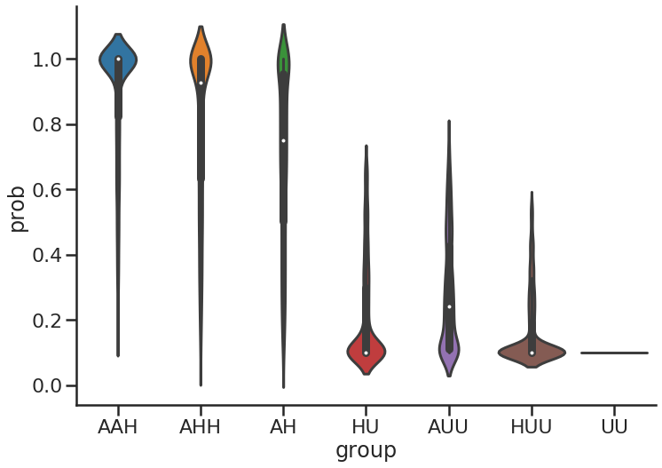
The average probabilities remain almost identical to Table 1, but are strongly adjusted (crossing the 50% threshold) depending on the relative ordering of the events. For instance, two adverse events followed by a unhelper event (AAU sequence) will have lower probabilities relative to UAA sequence. The further away these events have occurred from the time of prediction (t=0), that is the further in the past, the less likely a positive label will occur. The temporal-adjusted probability distribution for each of the pathways is depicted in Figure 1.
3.2 Real-world medical claims dataset
The data is a 5% sample limited dataset of the entire Centers for Medicare and Medicaid Services (CMS) medicare fee for service (Part A and B) claims data from 2009 to 2012, with about 3 million unique beneficiaries containing information about medical events and claims such as diagnosis, procedures, admissions, discharges, and death. Standardized coding systems such as ICD-9, HCPCS, and CPT are used, and extracted for each patient from all healthcare settings, i.e. inpatient, outpatient, if available and consolidated. Other non-codified events including admissions, discharges and gaps in medical care were provided unique tokens.
The events were codified with different prefixes depending on type. ICD-9 diagnosis events were coded in the format of ”d_” followed by the code; ICD-9 procedures as ”p_” and HCPCS procedures as ”h_”. Gaps in medical care were codified in the format of ”N_days”, where N refers to the numbers of days without any medical event activity between the last and next event. The events were ordered chronologically with same day events ordered randomly. Target event of interest is the Clostidium Difficile (C.Diff) infection and coded via ICD-9 diagnosis code of 00.845. Our choice of C.Diff infection event is due to the clinical significance and urgency of reducing in-hospital C.Diff infections as jointly stated by the Centers for Disease Control and Prevention and CMS.
We chose to forgo elaborate feature engineering to philosophically mimic the experimental design of many prior deep learning approaches, including those previously mentioned approaches from Rajkomar et al. (2018), Zhang et al. (2018), and Rasmy et al. (2020). All beneficiaries who had a primary hospitalization admission have at least one medical event are included. We additionally identified a list of potential risk factors (events) that lead to or cause C.Diff infection, and this was achieved by curating existing literature and clinicians inputs. Similar to the synthetic dataset driver events, we used the risk factors as our ground truth. Finally, we include all medical events identified as risk factors and events having at least 1000 occurrences in the dataset leading to a vocabulary of about 1000 medical events. Almost half of the selected events are the risk factors. The train set contains 1.4M observations while the validation and test sets contain around 248K observations each.
4 Methods
There are three degrees of freedom in this experiment: model, dataset and explainability method. We explore a traditional ML model (XGBoost) and a deep learning model (LSTM); an event-driven, sequence-driven, and real-world dataset; and for explainability: SHAP (both models), LRP(LSTM) and Attention (LSTM). For synthetic dataset, we explore both simple dot-product attention and self-attention and only dot-product attention for real-world dataset. For explainability, we quantify both global (overall feature importance) and local (per patient feature importance).
4.1 Data preprocessing
Different data preprocessing steps were applied depending on the target model. LSTM models can ingest variable sequences of events. The unique tokens form a vocabulary, with each token is assigned a unique index number. This sequence of indices are directly passed in batches to LSTM models for training and inference. XGBoost models cannot ingest sequences of variable lengths. Feature space is determined by the unique number of tokens in the entire dataset. And then each sequence is mapped to the feature space with the value in each dimension being the sum of occurrences of that token. Thus, all tokens or inputs are always made available to the model, with 0 encoding used to denote the absence of a token in the sequence. The real-world dataset requires additional preprocessing. For patients who received at least 1 medical event and had a primary hospitalization admission, up to 30 day’s worth of medical events were captured. The choice of 30 day’s was selected because longer history of data did not improve model performance. The events were captured relative to a 30-day forecasting window of interest. For example, if the forecasting window was January 1 2011, then the events prior to that date are captured. Additionally, the data is highly imbalanced with only less than 1% positive examples. We used stratified sampling to ensure representative distribution of positive examples in validation and test sets, and down-sampled observations with negative labels in training dataset.
4.2 Models, Methods and Metrics
Models Gradient boosting utilizes an ensemble of weak models to solve supervised ML problems, with gradient boosted trees using decision trees as weak learners. XGBoost (eXtreme Gradient Boosting) is a highly efficient and scalable implementation of the gradient boosted trees algorithm. Long Short-Term Memory (LSTM) networks are a type of recurrent neural networks (RNNs) capable of learning from long sequences of data. Unlike feed-forward neural networks, RNNs utilize internal hidden states to represent information from previous events in the sequence. Attention mechanisms are often added to the LSTM model architecture, which assists the model in selectively attending to specific events in the input sequence. We utilize the simplest dot-product attention and self-attention, and normalized attention scores are computed for each tokens in the sequence.
Training and Validation of Models Final models are decided using best AUC on validation set, which is the current widely used approach. We show later that this may not be the optimal approach for explainability, and that explainability performance during training as part of stopping criterion is also important. For speed purposes, a subset of 128-350 observations from the validation dataset is used to compute ground set truth similarities using the iterative SHAP and LRP explainability approaches but full validation and test sets are evaluated with the final models for AUC and explainability performance in synthetic datasets. For CMS dataset, we evaluated explainability on all positive observations (160 in test set) and a down-sampling of negative observations for a total of 800 observations due to compute time.
SHapley Additive exPlanations (SHAP) was developed by Lundberg and Lee (2017) based on a general idea of approximating the original complex model with a simpler explanation model. SHAP is categorized as an additive feature attribution methods, as the explanation model is linear and can easily tell the effect of each feature for each prediction. The classic Shapley value is derived using classic equations from cooperative game theory, which is a weighted average of the all possible marginal differences of model output by adding the presence of the examined feature to subsets of features. We use a background of 300 observations from training dataset to compute SHAP values.
Layer-Wise Relevance Propagation (LRP) is originally developed to relate the input images pixels to the final prediction of the neural network. The concept is expanded into multiple domains which follow the general form that the classifier can be decomposed into several layers of computation. Such decomposition can be either achieved through relevance score back propagation or Taylor expansion. Since the model output can be approximated with a linear function of non-linear mappings of the original input through neuron activation, it can be interpreted as an additive feature attribution method as well.
Attention scores Besides offering super-human performance on many language understanding tasks, attention-based methods are being used to estimate feature importance. Škrlj et al. (2020) showed that Self-Attention Network (SAN) was able to identify feature interactions on a much larger feature subsets compared to the commonly used methods. In our case, the normalized dot-attention scores inherent in the LSTM model are extracted on a per patient basis for local feature importance comparisons, and we additionally explore self-attention models in the synthetic dataset.
Metrics: Set similarity to ground truth for local explainability We evaluate the models’ ability to provide explainability at the per patient level. This comparison is performed on a set similarity basis, where we measure the overlap of top N important features between the SHAP output and the N ground truth drivers of these events. This set similarity metric is calculated on a per patient basis, and then averaged over the entire validation dataset. Set similarity = 1.0 means that all the important drivers were correctly identified in every patient, while zero similarity indicates that none of the key event drivers were correctly identified. Note that the ground truth set for XGBoost and LSTM models are different, as XGBoost includes the entire 45 tokens while LSTM models only see the active sequence, i.e. tokens that correspond to one in the XGBoost input space. Predictive performance is evaluated using AUC metric.
5 Results on Synthetic Experiments: Event-driven dataset
We summarize findings on predictive performance, global feature importance for overall model explainability and local feature importance for per-patient explainability.
Prediction Performance As the event-driven dataset does not depend on the sequential ordering of tokens and is only influenced by the presence or absence of a set of tokens, the modeling is relatively simple and the prediction performance (AUC) of both models are comparable. Best AUC results from training, validation and test sets are shown for both models in Table 2 where AUC results reach beyond 0.8 using this event-driven dataset. For both models, the highest AUC epoch is evaluated for explainability.
| Model | Dataset | Training AUC | Validation AUC | Test AUC |
|---|---|---|---|---|
| XGBoost | Event-driven | 0.8821 | 0.8174 | 0.8177 |
| LSTM | 0.8112 | 0.8249 | 0.8278 | |
| XGBoost | Sequence-driven | 0.8970 | 0.8282 | 0.8321 |
| LSTM | 0.8623 | 0.8706 | 0.8763 |
Global explainability Majority of negative labels contains unhelper (U) tokens (see Table 1) compared to those with positive labels due to the designed pathways, and these tokens are expected to have the highest or close to highest importance in the ranking of global features. Adverse (A) tokens should have similar importance or follow very closely next in ranking, as they are predictors of the positive labels but can also be reduced in impact by the presence of unhelper (U) tokens (30% probability of positive label when paired with 2 Us). Helper (H) tokens should be a distant third ranked group, as they are present in majority of the pathways while noise (N) tokens will be last due their lack of predictive power. In summary, the order of set of tokens should be a mix of (U’s, A’s), H’s, and finally N’s (non-information containing).
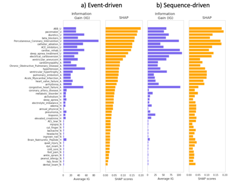
For the XGBoost model, the relative influence of the 45 tokens is well aligned with the known event drivers. Figure 2a) summarizes the global importance calculated using absolute SHAP scores, and plotted against global feature importance based on average information gain (IG). As with SHAP, the IG token classes were generally ordered correctly but the exact ordering between the tokens differ. The demarcation between information-containing and noise tokens is not clear with SHAP, but a cutoff can be fairly easily applied via IG.
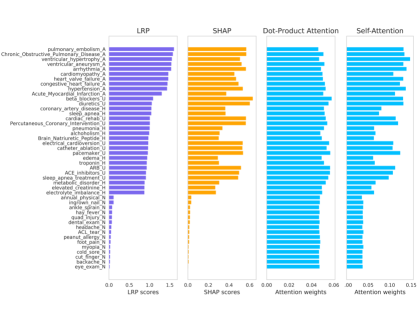
For the LSTM model, the four different approaches (SHAP, LRP, Dot-Product Attention and Self-Attention) to global model explainability is shown in Figure 3. For LRP, the set of adverse (A) tokens dominate explainability, followed by intermixing of unhelper (U) and helper (H) tokens. Noise tokens are correctly attributed with negligible importance. For explainability by SHAP values, the most important tokens are a mix of (A, U) tokens followed by helper tokens, and also assigns correctly little value to noise tokens. Dot-product attention’s feature importance is almost uniform across all tokens, and does not provide meaningful discrimination. Self attention provides better discrimination between useful and noise tokens than dot-product attention.
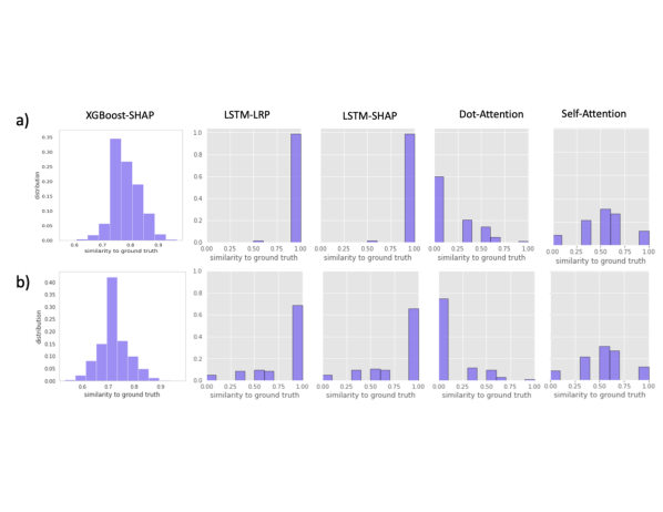
Local explainability The statistics (mean, range) applied to the test dataset for set similarity scores is reported in Table 3. Unlike LSTM, every feature or token is considered per observation with XGBoost and is compared against the existing 30 information-containing tokens. The distribution of set similarity scores per patient for LSTM is much more discrete than XGBoost, since there is at most 3 driver tokens at any sequence. Both LRP and SHAP are able to identify the information-containing tokens from the noise tokens very well, while attention scores often failed to do so. The score distribution is shown in Figure 4a).
| Metric | Dataset |
|
|
|
|
|
||||||||||
|---|---|---|---|---|---|---|---|---|---|---|---|---|---|---|---|---|
| Mean | Event- driven | 0.79 | 0.993 | 0.993 | 0.178 | 0.85 | ||||||||||
| Range | [0.567, 0.933] | [0, 1] | [0, 1] | [0, 1] | [0, 1] | |||||||||||
| Mean | Sequence- driven | 0.723 | 0.805 | 0.818 | 0.117 | 0.526 | ||||||||||
| Range | [0.533, 0.933] | [0, 1] | [0, 1] | [0, 1] | [0, 1] |
6 Synthetic dataset: Sequence-driven dataset
Prediction Performance Due to the sequential nature, whereby the relative ordering of the tokens and recentness of tokens affect the label probability, we observe performance differences between XGBoost and LSTM in the sequence-dataset section of Table 2.
Global explainability The added time dependencies results in a significant spread in label probabilities used to create the data (Figure 1). It is expected that the adverse (A) and unhelper (U) events to dominate, but with more intermixing due to the time-dependencies. The models should be able to separate noise from other informative tokens.
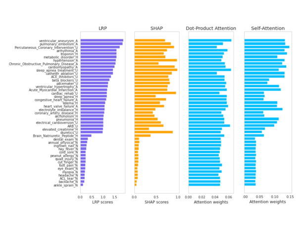
For the XGBoost model, the relative influence of the adverse and unhelper tokens are correctly identified but struggles to separate the helper tokens from the noise. Figure 2b) summarizes the global importance via SHAP and IG for sequence-driven dataset. For the LSTM model, global model explainability via LRP and SHAP continue to be accurate, and is shown in Figure 5. There is significant intermixing of the tokens as expected but the demarcation between noise and informative tokens is clear. Dot-product attention’s feature importance does not provide meaningful discrimination, with self-attention displaying discriminative ability between information and noise tokens, but with less clear demarcations compared to LRP or SHAP.
Local explainability Local explainability performance on the test set is summarized in the bottom half of Table 3. LSTM’s explainability performance via SHAP and LRP are higher than XGBoost. Distributions of this per patient explainability performance is shown in Figure 4b), where a majority of the explanations per patient was correct, and skewed by a minority of observations for LSTMs with SHAP or LRP. Self-attention continues to outperform dot-product attention.
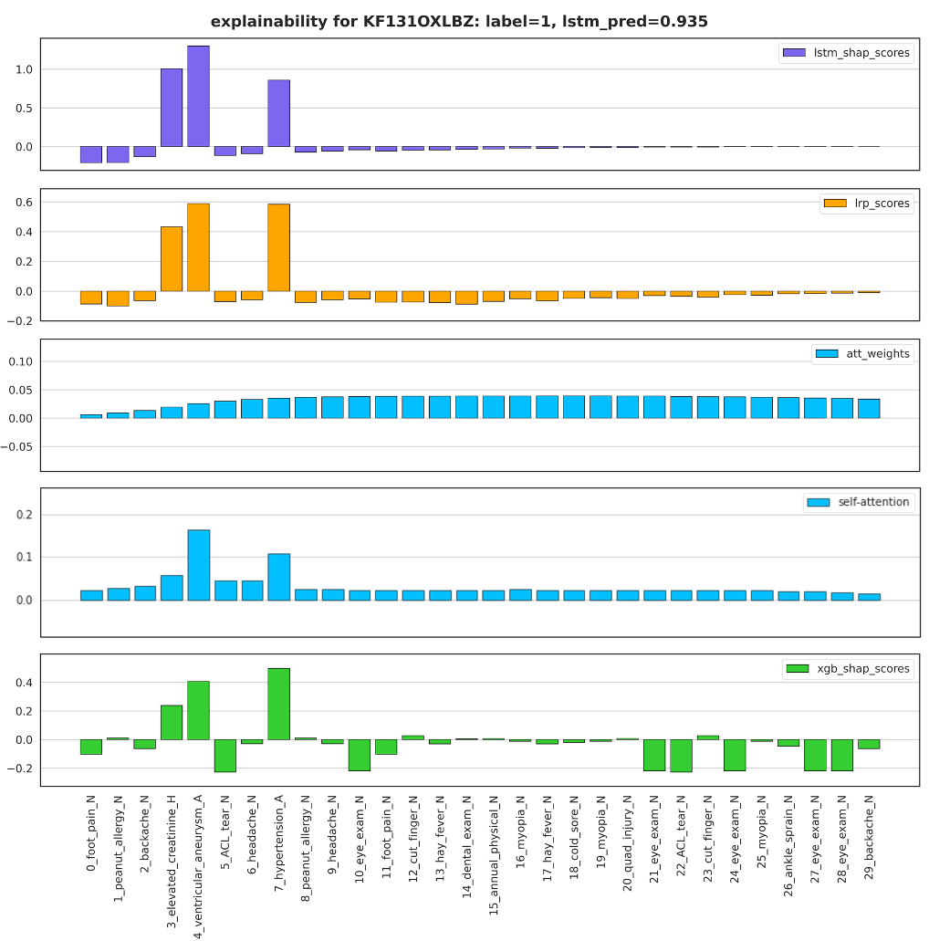
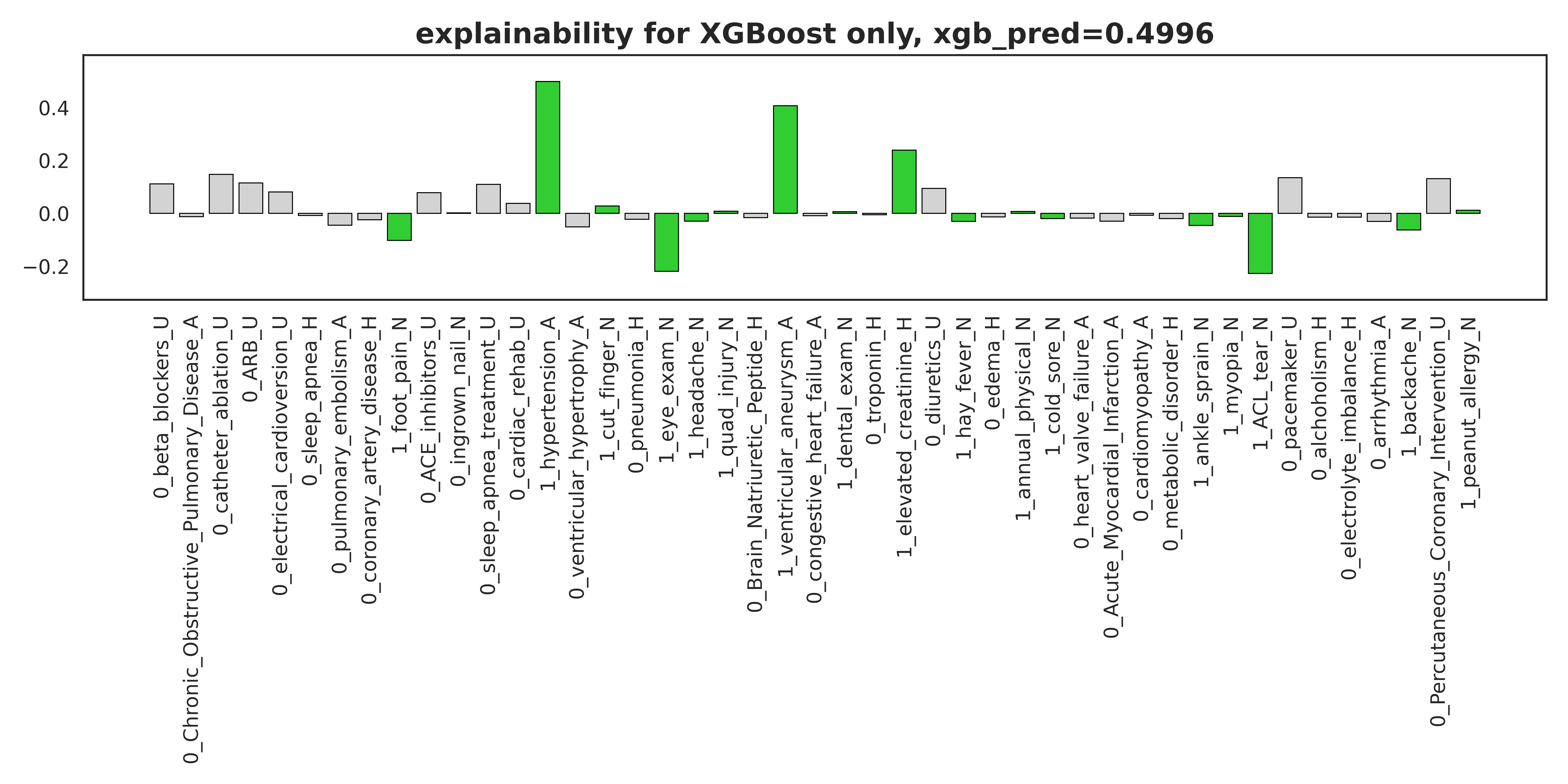
A full example of sequences with local explainability on sequence-driven data is shown in Figure 6. The top five figures correspond to the actual sequence of tokens or events and the relative importance scores assigned by LSTM-SHAP, LSTM-LRP, LSTM-Dot-Attention, LSTM-Self-Attention and XGBoost-SHAP. All the importance tokens were correctly identified. The x-axis denotes the combination of (sequence index, token, category), with 0_foot_pain_N being the first token of event foot_pain from the noise (N) category. The lowest figure denotes the full input feature space into the XGBoost model, which includes absence of tokens and highlights the inherently different input feature space encountered by both models. Positive events in green correspond to the earlier plot, which only displayed events that occurred. Some SHAP values were attributed to the non-occurring tokens, indicating that the sequential-ness of the tokens affect XGBoost’s ability to predict correctly, and noise tokens such as eye_exam were inaccurately attributed.
6.1 Evolution of explainability during model training
For XGBoost model during training on both synthetic datasets, we noticed a trend of improved explainability performance followed by a decrease. For the sequence-driven dataset in Figure 7a, Epoch 11 has the best explainability performance among all epochs with a set similarity of 0.764 on validation set. The highest AUC would be in epoch 19, which provided a reduced set similarity score of 0.723 or roughly 5% reduction in explainability. Visually, the optimal trade-off would be around Epoch 12.

We did not observe similar trends for the LSTM model for the set of model parameters and learning rates used (hidden state dimension = 16, embedding dimension = 8, and slow learning rate = 0.0003) for model training, which is shown in Figure 7b for SHAP explainability and Figure 7d for LRP explainability. These values were arrived using recommendations for model training listed in discussion section for optimal predictive and explainability performance, and we note a high sensitivity of explainability on right-sizing the model, regularization and learning rate. When the model parameter space and learning rates are slightly too large, we do observe similar trends to that displayed by XGBoost. This is shown in Figure 7c, using hidden state dimension = 16, embedding dimension = 16, and learning rate = 0.001 (about 3x compared to ideal learning rate).
Additional reduction in learning rates and increases in regularization did not remove this trend for XGBoost. This serves to emphasize the importance of having some understanding of important tokens or features within the input space, and to incorporate the set similarity overlap between these known features and important model features during model training.
7 Results on Real Data: C.Diff prediction
Prediction Performance Predictive performance is summarized in Table 4.
| Model | Training AUC | Validation AUC | Test AUC |
|---|---|---|---|
| XGBoost | 0.9170 | 0.8772 | 0.9184 |
| LSTM | 0.9292 | 0.8932 | 0.9226 |
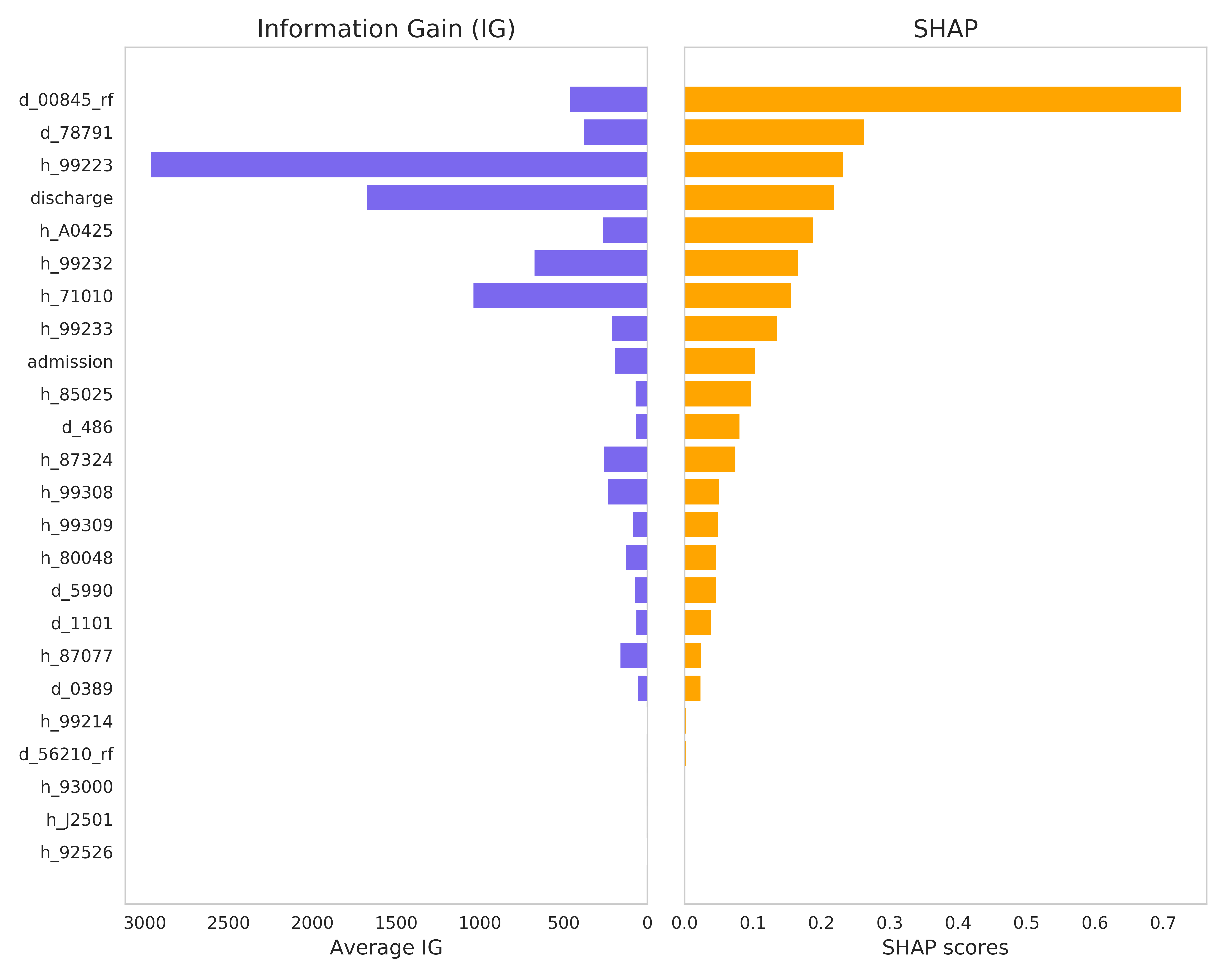
Global Explainability The global feature importance from the LSTM model is shown in Figure 8, using the best model identified over model training on validation data. Tokens that have suffixes of _rf are the identified risk factors from literature and clinicians. We find top 30 important tokens when predicting C.Diff infections by the model to be previously identified risk factors (12/30), gaps between times the patient receives medical care and hospital admission. The global feature importance by XGBoost is shown in Figure 9, and only 2 of the 24 top features were associated with previously known risk factors.
Among those top identified risk factors from the LSTM model, we see the ICD-9 ‘d_00845_rf’ diagnosis token, which refers to previous C.Diff infection. The ICD-9 ‘p_4601_rf’ procedure token refers to ‘Exteriorization of small intestine” and ‘p_4709_rf’ refers to an appendectomy. The HCPCS code ‘h_87324’ was not identified as a risk factor, and is lab result of ‘Infectious agent antigen detection by immunoassay technique’. The combination of these highlighted token paints a global picture that previous infections of C.Diff, along with bowel related procedures and confirmed lab tests were highly predictive of C.Diff diagnosis.

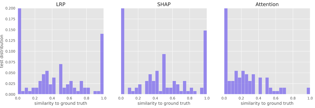
Local Explainability The set similarity metrics from SHAP, LRP and Dot-Attention with LSTM is shown in Figure 10. The patients without any identified risk factors and are excluded from calculations and distributions plots. The average set similarity for LRP, SHAP and Dot-Attention are 0.264, 0.305 and 0.017 and all with ranges of [0.0, 1.0]. Similar trends to synthetic data is observed, where attention scores underperform relative to LSTM-LRP and LSTM-SHAP. The high frequency of zero similarities originate from the fact that a good portion of patients had only one known risk factor and that the top feature identified by the model was not the single risk factor. The set similarity mean and range for XGBoost-SHAP is 0.45 and [0.419, 0.502]. Due to the CMS Data Use Agreements, individual explainabiltiy outputs cannot be shown.
8 Discussion
Strongly prevent over-fitting for explainability It is standard practice to utilize a validation set to determine optimal model parameters, and model with the highest predictive performance is selected for further use. First, we have shown that the model with highest explainability performance may not be the model with the best predictive performance. Thus, an optimal stopping point should be evaluated using both predictive metrics such as AUC and against known important features per epoch.
Secondly, the model tuning for explainability should be performed with care – with continued reduction of parameter dimensions and increase of regularization until noticeable degradation in predictive performance is observed. One can then conclude that the smallest parameter space has been found. This is particularly true for deep learning models, where the number of parameters or weights to be trained are often on the same order of magnitude as the available observations. We obtained similar predictive performances using a just-right model and a too-large model but with very different explainability performances, which may lead to wrong clinical conclusions.
Dot-product attention is not explainability Attention scores do not provide good overall explainability on global & locally, although it does accurately identify information-containing tokens in a small amount of examples and should not be used to provide explainability in a clinical setting.
Time-dependency of dataset An important aspect to model selection is to determine whether temporal dependencies exist with respect to the events driving the class label. When temporality exists or is uncertain, the LSTM model with SHAP or LRP explainability provides robustness in both 1) identification of global key features and 2) local explainability that can be provided to convince clinicians of correct model reasoning.
Separation of key features and noise For identification of global key features, the relatively sharp drop-off (Figure 5) in LSTM-SHAP and LSTM-LRP scores makes it relatively easy to distinguish between important and non-important features using either method. This is slightly less clear with XGBoost-SHAP alone, which captures majority of the overall important features but has trouble distinguishing between noise tokens and helper tokens. This gradual taper of SHAP scores makes it difficult to determine information-containing features as easily as the LSTM-SHAP/LRP combination. We note that if a traditional ML model must be utilized, one can leverage the comparatively sharp cutoff provided IG to distinguish between features containing information about the classification task and those that do not, but the better relative ordering between the tokens by SHAP indicate that the relative importance between features are better represented by SHAP than IG.
Use LSTM-SHAP or LSTM-LRP for local explainability The average set similarity between ground truth labels and model-identified features are highest using LSTM-SHAP or LSTM-LRP. When the temporality of the features is non-existent or weak, XGBoost-SHAP has the added value of explicitly considering the absence of a token as opposed to the implicit approach of LSTMs and may be useful in certain contexts. The choice between SHAP or LRP should be based on required inference time. SHAP scales with the number of background examples applied for each prediction which increases inference time, but there exists libraries for easy use of SHAP. Conversely, LRP back-propagation is custom and specific to each model definition and architecture but only needs to calculate the score back-propagation once per observation. In instances such as urgent care setting or during operative procedures where real-time evaluations are needed, it may be advantageous to invest resources upfront via LRP customization in exchange for low inference time. For other settings, such as classifications of patients for additional follow up care post-discharge, this difference in inference time does not make much difference.
Considerations for Real World Modeling Compared to the synthetic dataset, the real world results showed similar explainability characteristics in that known risk factors were identified by LRP/SHAP and some demarcation between events can be seen. However without a complete ground truth, interpreting the ”correctness” of the explainable outputs remains uncertain. Real world clinical ground truths can vary significantly depending on the clinician and presents challenges in optimizing model training for explainability. Known risk factors may not necessarily manifest depending on the individual and factors previously not considered relevant may later be discovered to be significant. This lack of a complete ground truth presents challenges on how to optimize a real world model for explainability.
Nonetheless, targeting good explainability remains important and we present several strategies to be explored to alleviate the challenges. If significant risk factors are unclear on the medical event level, then grouping risk factors and evaluating explainability on a class level could give directional feedback on its quality. It may also be easier to instead identify known noisy features and look for clear demarcation between the known noisy events and others. Smaller scale ground truth analysis from individual cases could also be validated through set similarity metrics looking at local explainability. Pertaining to the generalizability of LRP and SHAP, these methods can be ensembled, highlighting features universally agreed between different approaches.
Limitations
The input space we explored in the synthetic dataset was limited to 45 to ensure accurate and easy ground-truth comparison. In contrast, thousands of medical codes are currently in active use. Further work should be utilized to understand this in conjunction with the degradation of explainability performance when there are too many model parameters, as large vocabularies lead to learning exceedingly large number of embeddings. This is often addressed by grouping similar codes together using medical concepts.
The classification tasks in this study had relatively high AUC performances (above 0.8). It is unclear how our conclusions will change for lower performing models. We assume that explainability degrades with lower model performance, and further studies into the degree of degradation at different levels of performance are needed. We also focused on understanding the explainability performance of models on sequence-based, medical claims-like datasets. It is unclear how this would be extrapolated to other types of datasets like EHRs. Understanding derived from this work is extendable to simpler, less complex datasets.
This study does not include transformer models, which are best utilized with datasets larger than what was available in the real-world dataset. Existing transformer models are pre-trained on EHR datasets and cannot be leveraged for claims datasets. Finally, the multi-headed attention mechanism native to transformers does not fit the scope of our evaluation as they describe inter-feature relationships rather than feature-prediction relationships.
References
- Bach et al. (2015) Sebastian Bach, Alexander Binder, Grégoire Montavon, Frederick Klauschen, Klaus-Robert Müller, and Wojciech Samek. On pixel-wise explanations for non-linear classifier decisions by layer-wise relevance propagation. PLOS One, 2015. URL https://doi.org/10.1371/journal.pone.0130140.
- Bos et al. (2018) Jacqueline M. Bos, Gerard A. Kalkman, Hans Groenewoud, L. A. van den Bemt, Elsbeth Nagtegaal, and Gert Jan van der Wilt. Prediction of clinically relevant adverse drug events in surgical patients. PLoS One, P13(8): e0201645, 2018. URL 10.1371/journal.pone.0201645.
- (3) Centers for Disease Control and Prevention. What cdc is doing to reduce c. diff infections. URL https://www.cdc.gov/cdiff/reducing.html.
- (4) Centers for Medicare and Medicaid Services. Standard analytical files (medicare claims) - lds. URL https://www.cms.gov/Research-Statistics-Data-and-Systems/Files-for-Order/LimitedDataSets/StandardAnalyticalFiles.
- Farhan et al. (2016) W. Farhan, Z. Wang, Y. Huang, S. Wang, F. Wang, and X. Jiang. A predictive model for medical events based on contextual embedding of temporal sequences. JMIR medical informatics, 4(4), e39, 2016. URL https://doi.org/10.2196/medinform.5977.
- Jain and Wallace (2019) Sarthak Jain and Byron C. Wallace. Attention is not explanation. North American Chapter of the Association for Computational Linguistics, 2019. URL https://arXiv:1902.10186.
- Kaji et al. (2019) Deepak A. Kaji, John R. Zech, Jun S. Kim, Samuel K. Cho, Neha S. Dangayach, Anthony B. Costa, and Eric K. Oermann. An attention based deep learning model of clinical events in the intensive care unit. PLoS One, 2019.
- Lundberg and Lee (2017) Scott Lundberg and Su-In Lee. A unified approach to interpreting model predictions. arXiv preprint arXiv:1705.07874, 2017.
- Lundberg et al. (2018) Scott M Lundberg, Bala Nair, Monica S Vavilala, Mayumi Horibe, Michael J Eisses, Trevor Adams, David E Liston, Daniel King-Wai Low, Shu-Fang Newman, Jerry Kim, and Su-In Lee. Explainable machine-learning predictions for the prevention of hypoxaemia during surgery. Nature Biomedical Engineering, 2018. URL 10.1038/s41551-018-0304-0.
- Lundberg et al. (2019) Scott M Lundberg, Gabriel G. Erion, and Su-In Lee. Consistent individualized feature attribution for tree ensembles. ArXiv, 2019. URL https://arxiv.org/pdf/1802.03888.pdf.
- Meyer et al. (2018) Alexander Meyer, Dina Zverinski, Boris Pfahringer, Jörg Kempfert, Titus Kuehne, Simon H Sündermann, Christof Stamm, Thomas Hofmann, Volkmar Falk, and Carsten Eickhoff. Machine learning for real-time prediction of complications in critical care: a retrospective study. The Lancet Respiratory Medicine, 2018. URL 10.1016/S2213-2600(18)30300-X.
- Norrie (2018) John Norrie. The challenge of implementing ai models in the icu. The Lancet Respiratory Medicine, 2018. URL https://doi.org/10.1016/S2213-2600(18)30412-0.
- Rajkomar et al. (2018) Alvin Rajkomar, Eyal Oren, Kai Chen, Andrew M. Dai, Nissan Hajaj, Michaela Hardt, Peter J. Liu, Xiaobing Liu, Jake Marcus, Mimi Sun, Patrik Sundberg, Hector Yee, Kun Zhang, Yi Zhang, Gerardo Flores, Gavin E. Duggan, Jamie Irvine, Quoc Le, Kurt Litsch, Alexander Mossin, Justin Tansuwan, De Wang, James Wexler, Jimbo Wilson, Dana Ludwig, Samuel L. Volchenboum, Katherine Chou, Michael Pearson, Srinivasan Madabushi, Nigam H. Shah, Atul J. Butte, Michael D. Howell, Claire Cui, Greg S. Corrado, and Jeffrey Dean. Scalable and accurate deep learning with electronic health records. npj digital medicine, 1, 18, 2018. URL https://doi.org/10.1038/s41746-018-0029-1.
- Rasmy et al. (2020) Laila Rasmy, Yang Xiang, Ziqian Xie, Cui Tao, and Degui Zhi. Med-bert: pre-trained contextualized embeddings on large-scale structured electronic health records for disease prediction. ArXiv, 2020. URL https://arxiv.org/abs/2005.12833.
- Ross et al. (2019) Elsie Gyang Ross, Kenneth Jung, Joel T. Dudley, Li Li, Nicholas J. Leeper, and Nigam H. Shah. Predicting future cardiovascular events in patients with peripheral artery disease using electronic health record data. Circulation: Cardiovascular Quality and Outcomes, 12, No. 3, 2019. URL https://doi.org/10.1161/CIRCOUTCOMES.118.004741.
- Rudin (2019) Cynthis Rudin. Stop explaining black box machine learning models for high stakes decisions and use interpretable models instead. Nature Machine Intelligence, 2019. URL https://doi.org/10.1038/s42256-019-0048-x.
- Stiglic et al. (2020) Gregor Stiglic, Primoz Kocbek, Nino Fijacko, Marinka Zitnik, Katrien Verbert, and Leona Cilar. Interpretability of machine learning‐based prediction models in healthcare. WIREs Data Mining and Knowledge Discovery, 2020. URL https://doi.org/10.1002/widm.1379.
- Tonekaboni et al. (2019) Sana Tonekaboni, Shalmali Joshi, Melissa D. McCradden, and Anna GoldenbergAshish. What clinicians want: Contextualizing explainable machine learning for clinical end use. Proceedings of the 4th Machine Learning for Healthcare Conference, PMLR 106:359-380, 2019. URL http://proceedings.mlr.press/v106/tonekaboni19a.html.
- Wiegreffe and Pinter (2019) Sarah Wiegreffe and Yuval Pinter. Attention is not not explanation. Empirical Methods in Natural Language Processing, 2019. URL https://arXiv:1908.04626.
- Yang et al. (2018) Yinchong Yang, Volker Tresp, Marius Wunderle, and Peter A. Fasching. Explaining therapy predictions with layer-wise relevance propagation in neural networks. IEEE International Conference on Healthcare Informatics, 2018.
- Yoo et al. (2020) Tae Keun Yoo, Ik Hee Ryu, Hannuy Choi, Jin Kuk Kim, In Sik Lee, Jung Sub Kim, Geunyoung Lee, and Tyler Hyungtaek Rim. Explainable machine learning approach as a tool to understand factors used to select the refractive surgery technique on the expert level. Translational Vision Science and technology, 2020.
- Zhang et al. (2018) Jinghe Zhang, Kamran Kowsari, James H. Harrison, Jennifer M. Lobo, and Laura E. Barnes. Patient2vec: A personalizedinterpretable deep representation of the longitudinal electronic health record. IEEE Access, 0, 2018. URL https://arxiv.org/pdf/1810.04793.pdf.
- Škrlj et al. (2020) B. Škrlj, S. Džeroski, N. Lavrač, and M. Petkovič. Škrlj, b., džeroski, s., lavrač, n. and petkovič, m. Preprint at arXiv:2002.04464, 2020.