Abstract

Over the past several years, there has been enormous interest in massive neutron stars and white dwarfs due to either their direct or indirect evidence. The recent detection of gravitational wave event GW190814 has confirmed the existence of compact stars with masses as high as $\sim$2.5–2.67$M_{\odot}$ within the so-called mass gap, indicating the existence of highly massive neutron stars. One of the primary goals to invoke massive compact objects was to explain the recent detections of over a dozen Type Ia supernovae, whose peculiarity lies with their unusual light curve, in particular the high luminosity and low ejecta velocity. In a series of recent papers, our group has proposed that highly magnetised white dwarfs with super-Chandrasekhar masses can be promising candidates for the progenitors of these peculiar supernovae. The mass-radius relations of these magnetised stars are significantly different from those of their non-magnetised counterparts, which leads to a revised super-Chandrasekhar mass-limit. These compact stars have wider ranging implications, including those for soft gamma-ray repeaters, anomalous X-ray pulsars, white dwarf pulsars and gravitational radiation. Here we review the development of the subject over the last decade or so, describing the overall state of the art of the subject as it stands now. We mainly touch upon the possible formation channels of these intriguing stars as well as the effectiveness of direct detection methods. These magnetised stars can have many interesting consequences, including reconsideration of them as possible standard candles.

https://doi.org/10.3390/particles5040037 5 4 493-513 Academic Editor: Armen Sedrakian Received: 9 August 2022; Accepted: 30 August 2022; Published: 17 November 2022 yes Formation, Possible Detection and Consequences of Highly Magnetized Compact Stars Banibrata Mukhopadhyay ^1,∗,† and Mukul Bhattacharya ^2,∗,† Correspondence: bm@iisc.ac.in (B.M.); mmb5946@psu.edu (M.B.); Tel.: +91-80-2360-7704 (B.M.); Tel.: +1-512-293-7935 (M.B.); These authors contributed equally to this work. Mukul Bhattacharya and Banibrata Mukhopadhyay

1 Introduction

In the last several years, there has been much interest in massive compact objects. Sometimes the evidence is direct; however, it is indirect on some other occasions. For instance, the detection of gravitational wave (GW) event GW190814 Abbott2020 directly confirms the existence of a compact star with a mass of 2.5–2.67$M_{\odot}$. Thus far, the minimum mass of an astrophysical black hole is understood to be around $3M_{\odot}$ mac ; pooley (also see ozel ) while the maximum mass of a neutron star (NS) is argued to be about $2.5M_{\odot}$ alsing , leading to a so-called mass gap. Therefore, the above observation fills in the gap, arguing the compact object to be a massive NS. Note, however, that some researchers also claim against this mass gap. There indeed can be a depression in mass distribution. Nevertheless, there is other evidence for massive NSs (although not as massive as that inferred from GW190814) based on pulsar observations Cromartie2020 with mass $>2M_{\odot}$. Indeed, the statistics based on observation showed that while the averaged mass of NSs is about $1.4M_{\odot}$, the accreted millisecond pulsars have masses, on average, of $1.6M_{\odot}$ pul ; miller . Hence, there is no surprise with the discovery of more than two solar mass pulsars.

On the other hand, for more than 15 years, at least a dozen objects have been detected as peculiar over-luminous Type Ia Supernovae (SNeIa), whose unusually high luminosity, along with their violation of Khokhlov’s limit khok , argue for progenitor masses that are as high as $2.8M_{\odot}$ Scalzo2010 ; Howell2006 . This is evidence for a significant violation of the Chandrasekhar mass-limit of $\sim$1.4$M_{\odot}$ of white dwarfs (WDs) and a super-Chandrasekhar mass-limit.

An important question to ask is: how do we argue for the existence of such unconventional and massive compact objects? Numerous investigations have been carried out by our group aimed at uncovering this mystery over the last one decade. We have shown that strong magnetic field: its strength and anisotropic effect DM2012 ; DM2013 ; DM2013b ; DM2014 ; DM2015 ; SM2015 ; MB2018 ; MB_euro2018 ; AG2020 ; MB2021 ; MB2022 , modified Einstein’s gravity Ban2017 ; EPL2019 , and matter encountering noncommutative physics at high density in the core of compact stars IJMPD2020 ; IJMPD2021 can each independently lead to highly massive WDs and NSs. After our initiation, several other groups independently started looking at this issue based on other ideas, e.g., the ungravity effect BertM2016 , WDs having net electric charge Liu2014 ; Car2018 , lepton number violation Belyaev2015 and anisotropic pressure HB2013 . Additionally, there appears to be a relation between equation of state (EoS) and compact mass glen .

Magnetic fields in WDs and NSs, in general, degenerate stars, have been explored for a long time (see the review cham from three decades ago). In general, it is not difficult to understand the surface field of WDs and NSs to be $\sim$$10^{9}$ and $10^{15}$ G, respectively cham ; fw2005 , based on their different origins, e.g., fossil effect, dynamo, binary evolution etc. fw2000 ; fwk . Spectropolarimetric observations suggest that the magnetic flux of majority magnetic WDs is similar to that of main-sequence Ap-Bp stars fw2005 . This argues for an evolutionary link of magnetism between the main sequence stars and WDs. A similar argument can be made for isolated NSs if the underlying O-type progenitors have effective dipolar fields $\sim$$10^{3}$ G fw2005 . It has been statistically found that magnetic WDs are, in general, massive, and their number with fields at high as $\sim$$10^{9}$ G could even be $10\%$ of the total population fwk . However, magnetic field evolutions for isolated and accreting WDs are different. This is no surprise because in the outer layers of WDs, the field structure is expected to be modified due to accretion, particularly above a critical accretion rate rate $\approx\text{(1--5)}\times 10^{-10}M_{\odot}{\rm yr}^{-1}$. This results in a shorter Ohmic decay time, leading to an apparent lack of field $\sim$$10^{9}$ G in observed accreting WDs Cumming2002 ; zwf .

Among other consequences of magnetized and modified gravity-induced WDs are WD pulsars. These stars can also behave as soft gamma-ray repeaters (SGRs) and anomalous X-ray pulsars (AXPs) MR2016 ; BM2016 ; BM2019 , generating significant gravitational radiation that can be detected by space-based detectors Kalita2019 ; Kalita2020 ; Kalita2021 . Many of these transients can eventually turn out to be WDs with super-Chandrasekhar masses. Observational data from the Sloan Digital Sky Survey (SDSS) suggest that magnetic WDs can have larger masses compared to their non-magnetic counterparts, although they span the same temperature range Van2005 ; Ferrario2015 . Regardless of the rotation rate, strong magnetic fields have been shown to modify the EoS of electron degenerate matter and yield super-Chandrasekhar WDs with masses up to $\sim$$2.6\,M_{\odot}$ DM2012 ; DM2013 ; DM2013b ; SM2015 .

The effect of strong magnetic fields on the mass-radius relation has been explored previously by our group for both Newtonian DM2012 and general relativistic DM2014 ; SM2015 ; DM2015 ; MB2021 formalisms. These studies were performed for various different field configurations and were in good agreement with the results from independent studies Bos2013 ; FS2015 ; Car2018 . All the above ventures, including the underlying observations, by the aforementioned groups have brought super-Chandrasekhar WDs into the limelight in recent times. Magnetized WDs (B-WDs) have many important implications other than their apparent link to peculiar SNeIa, and, therefore, their other properties should also be explored MR2016 ; BM2016 . Strong magnetic fields can influence the thermal properties of WDs, namely their luminosity, temperature gradient and cooling rate MB2018 ; AG2020 ; MB2021 ; MB2022 . Moreover, the magnetic field of WD has a crucial role in their binary evolution as progenitors of SNeIa or accretion-induced collapse imin1 ; imin2 ; imin3 . Additionally, a possible merger through binary evolution leading to a peculiar SNeIa could be an alternate explanation for super-Chandrasekhar progenitors imin4 .

In this review paper, we discuss the broad implications of these compact stars as well as the current status of observations. We aim at gathering all the underlying results obtained in last decade or so and try to assess the overall state of the art of the subject as it stands now, in particular regarding the effects of magnetic fields in NS and WD. This paper is organised as follows. In Section 2, we discuss the origin and evolution of strong magnetic fields inside WD stars. In Section 3, we simulate the rotating and magnetized B-WDs based on their structural stability for toroidal and poloidal magnetic field geometries. In Section 4, we compute the mass-radius relation for non-rotating B-WDs, assuming a spherical geometry and radially varying field strength. In Section 5, we explore the effect of cooling as well as magnetic field dissipation on the modified mass limit and the suppressed luminosities of B-WDs. In Section 6, we briefly describe the quantisation of energy states of matter in B-WDs and derive their modified mass limit, assuming both constant and varying magnetic fields. In Section 7, we investigate the GW emission originating from WDs with misaligned rotation and magnetic axes, along with their detection prospects. Finally, we discuss the effect of anisotropy of dense matter in the presence of strong magnetic fields on the properties of B-WDs in Section 8 and conclude in Section 9.

2 Origin and Evolution of Magnetic Fields inside White Dwarfs

Here, we discuss the origin of strong fields inside magnetised WDs and their evolution at the end of the main sequence during the asymptotic giant phase. We present both numerical results from the Cambridge stellar evolution code STARS and analytical estimates from virial theorem that provide a relation between various energy components of the WD.

2.1 Origin of Magnetic Field

Magnetic fields in stars exhibit complex behaviour with structure on both small and large scales. The origin of large-scale fields is debated. They can be fossil fields (e.g., DM2013b ; fw2005 ) that can be dated back to the formation of the star or fields generated by a dynamic effect. Additionally, the field can be generated due to WD mergers (e.g., fw2005 ). As large-scale magnetic fields in stars can be unstable, dynamo effects are interesting because they can regenerate these fields. It is well known that purely poloidal or toroidal fields in stars are both structurally unstable MT1973 ; Tayler1973 . However, magnetized stars and B-WDs with a toroidally dominated mixed field configuration, along with a small poloidal component, are among the most plausible cases Wick2013 and also have an approximately spherical shape SM2015 . Unlike the surface magnetic field, which can be observationally inferred, fields in the interior of the WD cannot be directly constrained. However, there is a sufficient evidence that stars exhibit dipolar fields in their outer regions and are expected to have stronger toroidally dominated fields in their interior. Numerical simulations have already shown that the central fields of B-WDs can be several orders of magnitude higher than those at the surface SM2015 ; BM2017 ; QT2018 .

2.1.1 Dynamo-Model Based STARS Simulations

The evolution of magnetic field components along with the angular momentum during stellar evolution has been modelled recently with the Cambridge stellar evolution code STARS QT2018 using advection-diffusion equations coupled to the structural and compositional equations. It has been shown that the magnetic field is likely to be dipolar in nature, decaying as an inverse square law for most of the star. The simulation results also suggest that, at the end of main sequence, stars have toroidally dominated magnetic fields. The authors reported QT2018 the evolution of toroidal field in the interior of the WD as a function of mass coordinate at various times in the end of main sequence after the exhaustion of helium nuclei in the core, i.e. during the asymptotic giant phase, as displayed in Figure 1 for completeness.

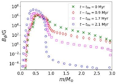
Figure 1: Toroidal field inside the star is shown as a function of the mass coordinate at various times after the helium exhaustion in the core, during the asymptotic giant phase. See QT2018 for details.

Large-scale magnetic fields can be present in the degenerate core of magnetised WDs or B-WDs; even during the late stages of stellar evolution QT2018 very high fields can develop based on the conservation of magnetic flux, as well as from the dynamo mechanism. Therefore, strong fields inside magnetized WDs can also be of fossil origin. While the mass of the WD increases due to accretion, the magnetic field is advected into its interior. Consequently, the gravitational power dominates over the degeneracy pressure, which leads to the contraction of the star. Hence, the initial seed magnetic field is amplified as the total magnetic flux remains conserved.

For magnetic field $B\sim 10^{8}\,{\rm G}$ within a star of size $R\sim 10^{6}\,{\rm km}$, the resultant flux will be $\sim$$10^{20}\,{\rm G\,km^{2}}$. From flux freezing, for a 1000 km size B-WD, the magnetic field can then grow up to $\sim$$10^{14}\,{\rm G}$. Once the field increases, the total outward force further builds up to balance the inward gravitational force, and the whole cycle is repeated multiple times. Therefore, the magnetic fields of B-WDs are likely to be fossil remnants from their main-sequence progenitor stars.

2.1.2 Modified Virial Theorem

Virial theorem relates the integrated gravitational potential, thermal, kinetic and magnetic energies of a physical system to provide insight into its equilibrium configuration. By invoking magnetic flux conservation and based on the variation of the internal magnetic field with the matter density as a power law, the modified virial theorem can be derived using the equation of magnetostatic equilibrium AS2021 . The well-known form of the virial theorem is

$$2T+W+3\Pi+\mu=0,$$ (1)

where $T$, $W$, $\Pi$ and $\mu$ are the kinetic, gravitational, thermal and magnetic energies, respectively. For the case of a static non-rotating WD, we have $T=0$. Assuming that a polytropic EoS is satisfied through the entire star such that $P=K\rho^{\Gamma}$, where $K$ and $\Gamma$ are polytropic constants, and $M=(4\pi/3)R^{3}\rho$ with $\rho$ is the mean density, the scalar virial theorem reduces to

$$-\alpha\frac{GM^{2}}{R}+\beta\frac{M^{\Gamma}}{R^{3(\Gamma-1)}}+\gamma\frac{\Phi_{M}^{2}}{R}=0.$$ (2)

After rearranging the terms, we obtain

$$M=\sqrt{\frac{\gamma\Phi_{M}^{2}}{\alpha G\left(1-\frac{\beta M^{\Gamma-2}}{\alpha GR^{3\Gamma-4}}\right)}}$$ (3)

for any $\Gamma$. For $\Gamma=4/3$, appropriate for extremely relativistic non-magnetic degenerate electrons, we obtain a mass which is independent of radius for a fixed magnetic flux, as expected from Chandrasekhar’s theory. We evaluate the coefficients $\alpha$, $\beta$ and $\gamma$ to establish the modified virial theorem for a high magnetic field.

In the presence of a strong magnetic field, the contribution of the magnetic pressure to the magnetostatic balance cannot be neglected. The new momentum balance condition, neglecting the effect of magnetic tension, is then given by

$$\frac{1}{\rho}\left(\frac{dP}{dr}+\frac{dP_{B}}{dr}\right)=-\frac{Gm(r)}{r^{2}}$$ (4)

at an arbitrary radius $r$ with mass enclosed at that radius $m(r)$, where $\rho$ includes the contribution from magnetic field and $P_{B}$ is the pressure due to the magnetic field of the star. We consider two different approaches to compute the modified virial theorem (see AS2021 ): (i) invoke flux conservation (freezing), which is quite common in stars when conductivity is high, and (ii) assume the magnetic field varies as a power law with respect to density, just as the EoS of thermal pressure, throughout.

For the case (i), the coefficients of the modified virial theorem are obtained as

$$\alpha=\frac{3(\Gamma-1)}{5\Gamma-6},\ \beta=\frac{3^{\Gamma}K}{(4\pi)^{\Gamma-1}},\ \gamma=\frac{2(n-1)}{5\Gamma-6}+\frac{4n-3}{6}.$$ (5)

For $n=1$, the situation simplifies to that of a non-magnetized or weakly magnetized WD or a B-WD with constant magnetic field and hence constant $P_{B}$ throughout. For power-law fields of case (ii), corresponding coefficients are

$$\alpha=\frac{3(\Gamma_{1}-1)}{5\Gamma_{1}-6},\ \beta=\left(1+\frac{\Gamma-\Gamma_{1}}{(5\Gamma_{1}-6)(\Gamma-1)}\right)\frac{3^{\Gamma}K}{(4\pi)^{\Gamma-1}},\ \gamma=\frac{1}{6},$$ (6)

where $\Gamma_{1}$ is the constant from the relation $P_{B}=K_{1}\rho^{\Gamma_{1}}$. It is important to note that $\alpha$ is related to the scaling of $B$ with $\rho$. Therefore, the presence of magnetic pressure allows either a more massive or smaller star. For $\Gamma=\Gamma_{1}$, the result reduces to that of the non-magnetic case with a redefined $K$. Figure 2 shows the variation of radius with indices $n$ and $\Gamma_{1}$ for the conserved flux and power-law field models, respectively, with various $\Gamma$ and total masses.

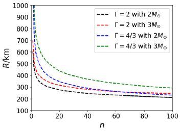
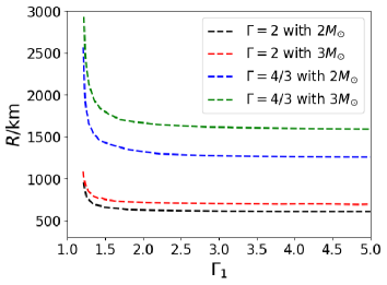
Figure 2: Left panel: Variation of radius with $n$ for the conserved flux model with various $\Gamma$ and total masses. Right panel: Variation of radius with $\Gamma_{1}$ for the power-law field model with various $\Gamma$ and total masses. In each case, $\Gamma=4/3$ corresponds to $\overline{B}=10^{14}\ {\rm G}$, and $\Gamma=2$ corresponds to $\overline{B}=10^{16}\ {\rm G}$, with $\overline{B}$ being the average magnetic field. Parameter sets from top to bottom mentioned in the figures correspond to the lines sequentially from bottom to top in the low $n$ and $\Gamma_{1}$ regimes. See AS2021 .

2.2 Evolution of Magnetic Field

Highly magnetised WDs can possibly result from repeated episodes of accretion and spin-down BM2017 . The entire evolution of the B-WD can be classified in two phases: accretion-powered and rotation-powered. The accretion-powered phase is governed by three conservation laws: linear and angular momenta conservation and conservation of magnetic flux around the stellar surface, given as

$$l\Omega(t)^{2}R(t)=\frac{GM(t)}{R(t)^{2}},\ I(t)\Omega(t)={\rm constant},\ B_{s}(t)R(t)^{2}={\rm constant},$$ (7)

where $l>1$ accounts for the dominance of gravitational force over the centrifugal force, $I$ is the stellar moment of inertia and $\Omega$ is the angular velocity of the star that also includes the contribution acquired due to accretion. Here, we neglect any possible field decay and assume a specific field geometry. Solving the above equations simultaneously gives the time evolutions of the radius, magnetic field and angular velocity during the accretion phase. Accretion discontinues when

$$-\frac{GM}{R^{2}}=\frac{1}{\rho}\frac{d}{dr}\left(\frac{B^{2}}{8\pi}\right)_{r=R}\sim-\frac{B_{s}^{2}}{8\pi R\rho},$$ (8)

where $\rho$ is the density of the inner disk edge.

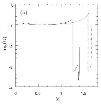
Figure 3: Time evolution of angular velocity (left panel) and magnetic field (right panel) as functions of mass. The solid curves correspond to the case with $n=3$, $m=2.7$, $\rho=0.05\,{\rm g\,cm^{-3}}$, $l=1.5$ and dotted curves correspond to the case with $n=3$, $m=2$, $\rho=0.1\,{\rm g\,cm^{-3}}$, and $l=2.5$. The other parameters are fixed with $k=10^{-14}$, $\dot{M}=10^{-8}\,M_{\odot}{\rm yr}^{-1}$, $\chi=10^{\circ}$ and $R=10^{4}\,{\rm km}$ at $t=0$. See BM2017 .

If the magnetic field is dipolar, $\dot{\Omega}\propto\Omega^{3}$ for a fixed magnetic field. Generalizing it to $\dot{\Omega}=k\Omega^{n}$ with constant $k$ giving for the spin-powered phase, we obtain

$$\Omega = [\Omega_{0}^{1-n}-k(1-n)(t-t_{0})]^{1/1-n},$$ (9)

$${\rm and}\,\,\,B_{s} = \sqrt{\frac{5c^{3}Ik\Omega^{n-m}}{R^{6}{\rm sin}^{2}\chi}}.$$ (10)

Here, $\Omega_{0}$ is the initial angular velocity for the spin-powered phase (once accretion stops) at time $t=t_{0}$, and $\chi$ is the angle between the rotation and magnetic axes. The value of $k$ is fixed such that $B_{s}$ can be constrained at $t=t_{0}$, which is known from the field evolution in the preceding accretion-powered phase. Here, $n=m=3$ corresponds to the dipole field configuration; therefore $m$ represents the deviation from the dipolar field, especially for $n=3$. Figure 3 shows the sample evolutions of angular velocity and magnetic field as functions of stellar mass. The initial angular velocity and particularly the magnetic field are chosen in such a way that they do not affect the stellar structure with respect to when they are zero. In both cases, initially larger $\Omega$ with accretion drops significantly during the spin-powered phase, followed by a phase of its increasing trend. At the end of the evolution, the star can be left either as a super-Chandrasekhar WD and/or an SGR/AXP candidate with a higher spin frequency. Other initial conditions do not produce qualitatively different results.

3 Simulating Magnetized and Rotating White Dwarfs and Their Stability

In nature, WDs are expected to consist of mixed field geometry, including both toroidal and poloidal magnetic field components. However, here we consider toroidally dominated magnetic fields as they ensure the stability of these stars. Note, in fact, that the core of WDs may contain a stronger toroidal field, which contributes to the stellar structure, mostly including mass, with a weaker surface poloidal field. We simulate WDs and B-WDs based on the Einstein equation solver, XNS code Pili2014 . It has been shown that toroidally dominated and purely toroidal fields not only make the star slightly prolate but also increases its equatorial radius KS2004 ; FR2012 ; SM2015 . It is seen that the deformation at the core is more prominent than the outer region. Nevertheless, the rotation of a star makes it oblate, and hence, there is always a competition between these two opposing effects to decide whether the star will be an overall oblate or prolate.

The combined effect of toroidal field and rotation (uniform and differential) was already explored in detail earlier Kalita2019 . It was shown that as the angular frequency is small, it does not affect the star considerably and results in a marginally prolate star due to magnetic effects. However, for high angular velocity, the low density region is affected more due to rotation than the high density central region, resulting in an oblate shaped star. For both the explorations, the magnetic to gravitational energies ratio (ME/GE) as well as kinetic to gravitational energies ratio (KE/GE) are chosen to be $\lesssim 0.1$ to maintain stable equilibrium ChF1953 ; Komatsu1989 ; Braithwaite2009 . The authors found that for the central density $\rho_{c}\sim 2.2\times 10^{10}\,{\rm g\ cm^{-3}}$, the magnetic field at the interior (close to the center) of the WD is $B_{max}\sim 2.7\times 10^{14}\,{\rm G}$. Several WDs are observed with the surface magnetic field $\sim 10^{9}\,{\rm G}$ Heyl2000 ; Van2005 ; Brink2013 ; hence, the central field might be much larger than $10^{9}\,{\rm G}$. In fact, it has already been argued in the literature that the central field could be as large as $10^{14}\text{--}10^{15}\,{\rm G}$ FS2015 ; SS2017 .

For differentially rotating B-WDs SM2015 , the angular velocity profile is specified as Ster2003 ; BDZ2011

$$F(\Omega)=A^{2}(\Omega_{c}-\Omega)=\frac{R^{2}(\Omega-\omega)}{\alpha^{2}-R^{2}(\Omega-\omega)^{2}},$$ (11)

which is implemented in the XNS code used to simulate them, where $A$ is a constant that indicates the extent of differential rotation, $R=\psi^{2}r{\rm sin}\theta$, $\omega=-\beta^{\phi}$, $\Omega_{c}$ is the angular velocity at the center and $\omega$ is the angular velocity at radius $r$. Previous works (e.g. DM2015 ; SM2015 ; Kalita2019 ) reported in detail the density isocontours of differentially rotating B-WDs for toroidal and poloidal fields. It was shown that ‘polar hollow’ structure can form with differential rotation regardless of the specific geometry of the magnetic field.

4 Mass-Limit and Luminosity Suppression in Non-Rotating White Dwarfs

Apart from increasing the limiting mass of WDs, strong magnetic fields can also influence the thermal properties of the star, such as its luminosity, temperature gradient and cooling rate MB2018 ; MB_euro2018 ; AG2020 ; MB2021 ; MB2022 . To model such a WD, the total pressure inside the star is modelled by including the contributions from the degenerate electron gas, ideal gas and magnetic pressures. The interface is at the radius where the contributions from electron degenerate core and outer ideal gas pressures are the same. The presence of strong fields gives rise to additional pressure $P_{B}=B^{2}/8\pi$ and density $\rho_{B}=B^{2}/8\pi c^{2}$ inside the magnetized WDs Sinha2013 when $c$ is the speed of light.

For an approximately spherical B-WD, the model equations for magnetostatic equilibrium, photon diffusion and mass conservation can be written within a Newtonian framework as

$$\frac{{\rm d}}{{\rm d}r}(P_{\rm deg}+P_{\rm ig}+P_{B})=-\frac{Gm(r)}{r^{2}}(\rho+\rho_{B}),$$

$$\frac{{\rm d}T}{{\rm d}r}=-{\rm max}\left[\frac{3}{4ac}\frac{\kappa\rho}{T^{3}}\frac{L_{r}}{4\pi r^{2}},\left(1-\frac{1}{\gamma}\right)\frac{T}{P}\frac{{\rm d}P}{{\rm d}r}\right],\vspace{0.1in}$$ (12)

$$\frac{{\rm d}m}{{\rm d}r}=4\pi r^{2}(\rho+\rho_{B}),$$

where we have ignored the magnetic tension term for radially varying magnetic field strength. In these equations, $P_{\rm deg}$ and $P_{\rm ig}=\rho kT/\mu m_{p}$ are the electron degeneracy pressure and the ideal gas pressure, $\rho$ is the matter density, $T$ is the temperature, $m(r)$ is the mass enclosed within radius $r$, $\kappa$ is the radiative opacity, $L_{r}$ is the luminosity at radius $r$, and $\gamma$ is the adiabatic index of the gas.

The opacity in the surface layers of non-magnetised WD is approximated with Kramers’ formula, $\kappa=\kappa_{0}\rho T^{-3.5}$, where $\kappa_{0}=4.34\times 10^{24}Z(1+X)\ {\rm cm^{2}\ g^{-1}}$, and $X$ and $Z$ are the mass fractions of hydrogen and heavy elements (other than hydrogen and helium) in the stellar interior, respectively. Assuming helium WDs for our study here, we set the helium mass fraction to $Y=0.9$ and $Z=0.1$. The radiative opacity in the surface layers is mainly due to the bound-free and free-free transitions of electrons ST1983 . For the radial variation of the field magnitude within the B-WD, we adopt a profile used extensively to model magnetized NSs and B-WDs Band1997 ; DM2014 , given by

$$B\left(\frac{\rho}{\rho_{0}}\right)=B_{\rm s}+B_{0}\left[1-{\rm exp}\left(-\eta\left(\frac{\rho}{\rho_{0}}\right)^{\gamma}\right)\right],$$ (13)

where $B_{s}$ is the surface magnetic field, $B_{0}$ is a fiducial magnetic field, and $\eta$ and $\gamma$ are dimensionless parameters along with $\rho_{0}=10^{9}\,{\rm g/cm^{3}}$, which determine how the magnetic field decays from the degenerate core to the surface. We set $\eta=0.8$ and $\gamma=0.9$ for all calculations, unless stated otherwise.

Radial luminosity is assumed to be constant, $L_{r}=L$, as there is no hydrogen burning or other nuclear fusion reactions that take place within the WD core. The differential equations are solved by providing the matter density at the surface, total WD mass and surface temperature as the boundary conditions. For strong magnetic fields, the variation of radiative opacity with $B$ can be modelled as $\kappa=\kappa_{B}\approx 5.5\times 10^{31}\rho T^{-1.5}B^{-2}{\rm cm^{2}\ g^{-1}}$ PY2001 ; VP2001 . The field-dependent Potekhin’s opacity is used instead of Kramers’ opacity if $B/10^{12}\ {\rm G}\geq T/10^{6}\ {\rm K}$, which is relevant for the strong fields that we consider.

The left panel of Figure 4 shows the effect of luminosity on the mass-radius relation for non-magnetized WDs compared to Chandrasekhar’s results Ch1935 . Although the increase in $L$ leads to progressively higher masses for larger WDs, Chandrasekhar mass limit is retained irrespective of the luminosity. The right panel of Figure 4 shows the effect of magnetic field on the mass-radius relation for B-WDs with $L=10^{-4}\,L_{\odot}$ and compares them with the non-magnetic Chandrasekhar results. It can be seen that the magnetic field affects the mass-radius relation in a manner analogous to increasing $L$ by shifting the curve towards higher masses for these WDs having larger radii. The mass-radius curves for $B_{0}\lesssim 10^{13}\,{\rm G}$ practically overlap with each other in the smaller radius regime and retain the Chandrasekhar mass limit. However, for strong central fields with $B_{0}\sim 10^{14}\,{\rm G}$, super-Chandrasekhar WDs are obtained, with masses as high as $\sim$$1.9\,M_{\odot}$.

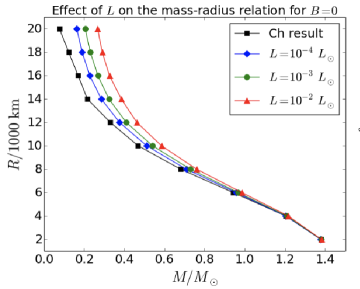
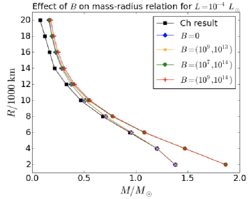
Figure 4: Left panel: The effect of $L$ on the mass–radius relation of non-magnetised WDs is shown for $L=10^{-4}\ L_{\odot}$ (blue diamonds), $L=10^{-3}\ L_{\odot}$ (green circles) and $L=10^{-2}\ L_{\odot}$ (red triangles), along with the Chandrasekhar result (black squares). Right panel: The effect of field strength on the mass–radius relation of B-WDs is shown for $B=(B_{s},B_{0})=(0,0)$ (blue diamonds), $B=(10^{9},10^{13})\ {\rm G}$ (orange crosses), $B=(10^{7},10^{14})\ {\rm G}$ (green circles) and $B=(10^{9},10^{14})\ {\rm G}$ (red pluses), along with the Chandrasekhar result (black squares) for $L=10^{-4}\ L_{\odot}$. See MB2022 .

To ensure structural stability of B-WD, an increase in magnetic energy density has to be compensated by a corresponding decrease in the thermal energy and hence the luminosity. This effect is especially prominent for B-WDs with larger radii where the magnetic, thermal and gravitational energies are comparable with each other. We find that in the presence of stronger field, a slight decrease in the luminosity for $R\gtrsim 12000\,{\rm km}$ WDs leads to masses that are similar to their non-magnetic counterparts. However, the smaller radius B-WDs require a substantial drop in their luminosity (well outside the observable range) and still do not really achieve masses that are similar to the non-magnetized WDs. As a result, for stars with $2000\leq R/{\rm km}\leq$ 10,000, even if the luminosity decreases substantially with $10^{-16}\leq L/L\leq 10^{-12}$, the resulting mass of the B-WD remains larger than its non-magnetic counterpart. This leads to an extended branch in the mass-radius relation.

5 Effect of Magnetic Field Dissipation and Cooling Evolution

Magnetic fields inside WD undergo decay by Ohmic dissipation and Hall drift processes with timescales given by HK1998 ; Cumming2002 , respectively,

$$t_{\rm Ohm}=(7\times 10^{10}\ {\rm yr})\,\rho_{c,6}^{1/3}R_{4}^{1/2}(\rho_{\rm avg}/\rho_{\rm c}),$$ (14)

$$t_{\rm Hall}=(5\times 10^{10}\,{\rm yr})\ l_{8}^{2}B_{0,14}^{-1}T_{\rm c,7}^{2}\rho_{\rm c,10},$$ (15)

where $\rho_{\rm c,n}=\rho_{c}/10^{n}\,{\rm g\,cm^{-3}}$, $R_{4}=R/10^{4}\,{\rm km}$, $T_{c,7}=T_{c}/10^{7}\,{\rm K}$, $B_{0,14}=B_{0}/10^{14}\,{\rm G}$ and $l=l_{8}\times 10^{8}\,{\rm cm}$ is the characteristic length scale of the flux loops through the outer core of WD. Ohmic decay is the dominant field dissipation process for $B\lesssim 10^{12}\ {\rm G}$, while for $10^{12}\leq B/{\rm G}\leq 10^{14}$, the decay occurs via Hall drift, and for $B\gtrsim 10^{14}\ {\rm G}$, the principal decay mechanism is likely to be ambipolar diffusion HK1998 .

The field decay can be solved using

$$\frac{{\rm d}B}{{\rm d}t}=-B\left(\frac{1}{t_{\rm Ohm}}+\frac{1}{t_{\rm Amb}}+\frac{1}{t_{\rm Hall}}\right),$$ (16)

where $t_{\rm Amb}$ denotes the ambipolar diffusion time scale. We consider two separate cases: (a) when only Ohmic dissipation occurs for both the surface and central magnetic fields, and (b) while $B_{s}$ continues to evolve over $t_{\rm Ohm}$, Hall drift determines the $B_{0}$ evolution until the central field drops to about $10^{12}\,{\rm G}$, below which Ohmic dissipation sets in.

The thermal energy is radiated away gradually over time in the observed luminosity from the surface layers as the star evolves. Because most of the electrons occupy the lowest energy states in a degenerate gas, the thermal energy of ions is the only significant energy source that can be radiated. The rate at which thermal energy of ions is transported to surface and radiated depends on the specific heat, given by

$$L=-\frac{d}{dt}\int c_{v}dT=(2\times 10^{6}\ {\rm erg/s)}\,\frac{Am_{\mu}}{M_{\odot}}\left(\frac{T}{K}\right)^{7/2},$$ (17)

where $c_{v}\approx 3k_{B}/2$ is the specific heat at constant volume. Given an initial $L$ and temperature $T_{0}$ at time $t_{0}$, final temperature after cooling is given by $(T/{\rm K})^{-5/2}-(T_{0}/{\rm K})^{-5/2}=2.406\times 10^{-34}\,\tau/{\rm s}$, where $\tau=t-t_{0}$ is the WD age. It is important to note that for simplicity in calculations, we have assumed self-similarity of the cooling process over the entire evolution.

Table 1 lists the luminosities and masses for WDs with radii $2000\lesssim R/{\rm km}\lesssim$ 20,000 and initial $B=(10^{9},10^{14})\,{\rm G}$ at time $t=0$ and $10\,{\rm Gyr}$. The fraction of time when the Hall drift dominates, i.e., $t_{\rm Hall}/\tau$, falls significantly with increasing stellar radius. Therefore, the magnetic field decays considerably more because the faster Ohmic dissipation process turns out to be critical for much of the cooling evolution. The mass-radius relations merge for $R\gtrsim 6000\,{\rm km}$ WDs. The inferred luminosities are also much less suppressed for the intermediate radius WDs with $6000\lesssim R/{\rm km}\lesssim 12000$. However, for low radius B-WDs, field decay affects mass and luminosity significantly. As it is the high magnetic pressure which helps to hold more mass, the field decay significantly sheds off mass in its new equilibrium if the radius is fixed. The limiting mass for small radius B-WDs with a fixed $R\approx 2000\,{\rm km}$ drops to about $1.5\ M_{\odot}$ due to field decay compared to $1.9\ M_{\odot}$ without field evolution. The majority of these small radius B-WDs still remain practically hidden throughout their cooling evolution because of their strong fields and correspondingly low luminosity.

Table 1: The effect of magnetic field on luminosity when the initial field is fixed at $B=(10^{9},10^{14})\ {\rm G}$ for all the radii. The topmost entry for each radius is the initial time, whereas the bottom two entries list corresponding parameters for $t=\tau=10\ {\rm Gyr}$. We evaluate fields assuming Ohmic dissipation is the dominant process for the top entries of $\tau=10\ {\rm Gyr}$, and for the bottom entries, we assume Hall drift is the primary process until the field parameter $B_{0}$ decays to $\sim$$10^{12}\ {\rm G}$, below which Ohmic dissipation dominates.

R/1000 km	$t/{\rm Gyr}$	$t_{\rm Hall}/\tau$	$B_{\rm s}/{\rm G}$	$B_{0}/{\rm G}$	$L/L_{\odot}$	$M_{B=0}/M_{\odot}$	$M/M_{\odot}$
2.0	0		$10^{9}$	$10^{14}$	$10^{-16}$	1.378	1.865
	10	0	$4.58\times 10^{8}$	$4.58\times 10^{13}$	$10^{-16}$	1.377	1.478
		1		$5.83\times 10^{13}$	$10^{-16}$		1.542
8.0	0		$10^{9}$	$10^{14}$	$10^{-12}$	0.709	0.762
	10	0	$9.86\times 10^{7}$	$9.86\times 10^{12}$	$2\times 10^{-6}$	0.699	0.699
		$2.28\times 10^{-2}$		$1.04\times 10^{11}$	$7\times 10^{-6}$		0.699
14.0	0		$10^{9}$	$10^{14}$	$2\times 10^{-6}$	0.286	0.286
	10	0	$3.06\times 10^{7}$	$3.06\times 10^{12}$	$10^{-5}$	0.262	0.262
		$2.22\times 10^{-3}$		$3.08\times 10^{10}$	$10^{-5}$		0.262
20.0	0		$10^{9}$	$10^{14}$	$7\times 10^{-6}$	0.164	0.164
	10	0	$2.97\times 10^{7}$	$2.97\times 10^{12}$	$10^{-5}$	0.138	0.138
		$3.70\times 10^{-4}$		$2.98\times 10^{10}$	$10^{-5}$		0.138

The left panel of Figure 5 shows the effect of B-WD evolution on their mass-radius relations, including both magnetic field decay and thermal cooling effects but neglecting neutrino cooling. The luminosities are varied with field strength such that the B-WD masses can match those obtained for the non-magnetized WDs. For $B=(0,0)\,{\rm G}$, the mass-radius relation is shifted more towards the Chandrasekhar result as a result of cooling, and the mass limit remains unaltered. However, for $B=(10^{9},10^{14})\,{\rm G}$, although the maximum mass $\sim$$1.9\,M_{\odot}$ at a small radius turns out to be much larger than the Chandrasekhar limit, we find that it is lowered considerably to $\sim$$1.5\,M_{\odot}$ primarily as a result of magnetic field decay and also thermal cooling over $t=10\,{\rm Gyr}$. The right panel of Figure 5 shows the radial variation of matter density for the same cases. Matter density at the core is slightly suppressed in the presence of strong field and also as a result of the evolution. As the total stellar energy is conserved, an increase in the magnetic energy has to be compensated by a similar decrease in gravitational energy, and, hence, the central density. Once the field decays and luminosity drops due to cooling, the central density adjusts itself to be slightly lower to balance the loss of magnetic and thermal energies with time.

We also use the STARS stellar evolution code to qualitatively investigate the B-WD mass-radius relationship at different field strengths, with the objective of numerically validating our semi-analytical models. We find that the numerical results are in good agreement with our analytical formalism, and the magnitude of $B_{0}$ dictates the shape of the mass-radius curve. In validation of our analytical approach, we have found that the limiting mass $\sim$$1.8703M_{\odot}$ obtained with the STARS numerical models is in very good agreement with $M\approx 1.87M_{\odot}$, which is inferred from the semi-analytical calculations for B-WDs with strong fields $B=(10^{\text{6--9}},10^{14})\,{\rm G}$ MB2022 for a given magnetic field profile.

We argue that the young super-Chandrasekhar B-WDs only sustain their large masses up to $\sim$$10^{5}\text{--}10^{6}\,{\rm yr}$ since their formation, and this essentially explains their apparent scarcity even without the difficulty of detection owing to their suppressed luminosities. We plan to explore this issue in detail in the future, particularly the timescale of their formation considering simultaneously the growth (e.g., by accretion BM2017 ) and decay of fields. It is important to note that if matter accretes at a higher rate such that the total mass accreted exceeds $\sim$0.1–0.2$M_{\odot}$ before the field diffuses, the field may be restructured zwf , leading to a reduced polar field independent of the initial field. We also plan to rigorously explore the fate of B-WDs once the fields decay, if they actually collapse, in place of keeping the radius fixed.

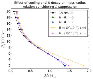
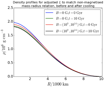
Figure 5: Left panel: Effect of magnetic field on $L$ set to match the non-magnetised mass-radius relation. Results are shown for $B=(0,0)$ at $t=0$ (green circles), $B=(0,0)$ at $t=10\ {\rm Gyr}$ (blue diamonds), $B=(10^{9},10^{14})\,{\rm G}$ at $t=0$ (orange triangles) and $B=(10^{9},10^{14})\,{\rm G}$ at $t=10\ {\rm Gyr}$ (magenta crosses). Right panel: The matter density profiles for the same cases are shown for R = 10,000 km. See MB2022 .

6 Mass Limit Estimate Including Quantum Effects

Several magnetized WDs have been discovered with surface fields as high as $\sim$$10^{5}\text{--}10^{9}\,{\rm G}$. It is likely that stronger fields ($\sim$$10^{12}\text{--}10^{14}\,{\rm G}$) exist at their interiors. Energy states of a free electron in a uniform strong magnetic field are quantized into Landau orbitals, which defines the motion of the electron in a plane perpendicular to the field. The maximum number of Landau levels occupied by cold electrons in a magnetic field is given by $\nu_{m}=\frac{(E_{Fmax}/m_{e}c^{2})^{2}-1}{2B_{D}}$, where $m_{e}$ is the rest mass of the electron, $E_{Fmax}$ is the maximum Fermi energy of the system and $B_{D}=B/B_{c}$, where $B_{c}=4.414\times 10^{13}\,{\rm G}$, is the critical field strength. High magnetic field strength therefore modifies the equation of state (EoS) of degenerate matter by causing Landau quantization of electrons LS1991 . The larger the magnetic field, the smaller is the number of Landau levels occupied DM2013 . This results in a significant modification of the mass-radius relation of the underlying WD, particularly for $B_{D}\gtrsim 100$.

To obtain the revised mass-radius relation for a strongly magnetized WD, the modified EoS has to be combined with the condition of magnetostatic equilibrium. If the B-WD is approximated to be spherical, then its mass is obtained from

$$\frac{1}{\rho+\rho_{B}}\frac{d}{dr}\left(P+\frac{B^{2}}{8\pi}\right)=-\frac{GM}{r^{2}}+\left[\frac{\vec{B}\ .\nabla\vec{B}}{4\pi(\rho+\rho_{B})}\right]_{r},\ \frac{dM}{dr}=4\pi r^{2}(\rho+\rho_{B}).$$ (18)

If the field is uniform or highly fluctuating, the magnetic terms can be neglected in the above equations, and following Lane–Emden formalism ARC2010 , the scalings of mass and radius with central density are obtained as

$$M\propto K_{m}^{3/2}\rho_{c}^{(3-n)/2n},\ R\propto K_{m}^{1/2}\rho_{c}^{(1-n)/2n},\ K_{m}=K\rho_{c}^{-2/3}.$$ (19)

Here, $n=1$ ($\Gamma=2$), which is the case for a high $B_{D}$ as shown in Figure 6, corresponds to central density independent mass, unlike Chandrasekhar’s case when $K_{m}$ is independent of the field strength, and limiting mass corresponds to $n=3$.

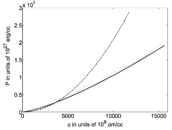
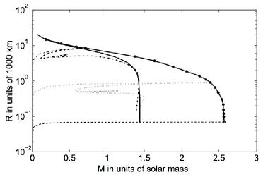
Figure 6: Left panel: EoS for different cases: solid line represents Chandrasekhar’s EoS, and the dotted and dashed lines represent the 5-level (corresponding to very strong $B$) and 1-level (corresponding to ultimate EoS for extreme $B$) systems of Landau quantization, respectively. Right panel: Mass-radius relations: pure solid line represents Chandrasekhar’s result, and the one marked with filled circles represents the evolutionary track of WD with an increase in $B$. The dot-dashed, dotted and dashed lines represent WDs with 50124-level, 200-level and 1-level systems of Landau quantization, respectively (corresponding to increasing $B$). We set $E_{Fmax}=200m_{e}c^{2}$ for both panels. See DM2013 ; DM2013b .

Substituting the proportionality constants appropriately, the limiting mass is obtained as

$$M_{lim}=\left(\frac{hc}{2G}\right)^{3/2}\frac{1}{(\mu_{e}m_{H})^{2}}\approx\frac{10.312}{\mu_{e}^{2}}M_{\odot},$$ (20)

when the limiting radius $R_{lim}\rightarrow 0$. For $\mu_{e}=2$, which is the case for a carbon-oxygen WD, we obtain $M_{lim}=2.58M_{\odot}$. For a finite but high-density and magnetic field, e.g., $\rho_{c}=2\times 10^{10}\,{\rm g\ cm^{-3}}$ and $B=8.8\times 10^{15}\,{\rm G}$ when $E_{Fmax}=20m_{e}c^{2}$, $M_{lim}=2.44M_{\odot}$ and $R\approx 650\,{\rm km}$. It should be noted that these $\rho_{c}$ and $B$ are similar or below their respective upper limits set by the instabilities of pycnonuclear fusion, inverse-$\beta$ decay and general relativistic effects DM2014 . Note, however, that pycnonuclear reaction rates are quite uncertain and not well constrained. Moreover, slightly lower $\rho_{c}$ and $B$ still would lead to B-WD mass well above the Chandrasekhar mass-limit.

The left panel of Figure 6 shows how the EoS of electron degenerate matter is modified as a result of magnetic field. With increasing field, the inward gravitational force is balanced by the outward force due to modified matter pressure, and a quasi-equilibrium state is attained. Consequently, with  decreasing stellar radius due to a higher gravitational field, a very high magnetic field is generated, which prevents the WD from collapsing, thus making its equilibrium configuration more massive. Subsequently, with the continuation of accretion the WD approaches the new mass limit $M_{lim}\sim 2.58M_{\odot}$. This new limiting mass WD plausibly sparks off a violent thermonuclear reaction with further accretion, as is the case with the idea of the $1.4M_{\odot}$ limit of nonmagnetic WDs, thus exploding it and giving rise to an over-luminous type Ia supernova.

The evolution of the mass-radius relationship with the evolution of magnetic field for a super-Chandrasekhar WD of maximum possible mass is shown in the right panel of Figure 6, along with a few typical mass-radius relations for different fixed magnetic field strengths describing possible stars in intermediate equilibrium states. The ultimate WD, corresponding to the maximum mass $M_{lim}\sim 2.58M_{\odot}$, lies on the mass-radius relation for a one-Landau-level system, but the intermediate WDs having weaker magnetic fields correspond to multilevel systems. The said one-Landau-level system corresponds to the hypothetical high central magnetic field $8.8\times 10^{17}\,{\rm G}$. This is in the spirit of a Chandrasekhar mass-limit for a non-magnetic WD, which also corresponds to the hypothetical high (even infinity) central density. However, the mass for $B_{D}\sim 30-100$ still appears to be significantly super-Chandrasekhar. The intermediate systems of 200-level and 50124-level systems correspond to central magnetic fields of $4.4\times 10^{15}\,{\rm G}$ and $1.7\times 10^{13}\,{\rm G}$, respectively.

7 Detectability of Gravitational Waves from Magnetised White Dwarfs

One question that remains to be answered is how can B-WDs be detected directly. Continuous gravitational waves can be among the alternate ways to detect super-Chandrasekhar WD candidates. If B-WDs are rotating with certain angular frequency, then they can efficiently emit gravitational radiation, provided that their magnetic field and rotation axes are not aligned BG1996 , and these gravitational waves can be detected by upcoming instruments. The dimensionless amplitudes of the two polarizations of a gravitational wave (GW) at a time $t$ are given by BG1996 ; ZS1979

$$h_{+}=h_{0}{\rm sin}\,\chi\,\left[\frac{1}{2}{\rm cos}\,i\,{\rm sin}\,i\,{\rm cos}\,\chi\,{\rm cos}\,\Omega t-\frac{1+{\rm cos}^{2}i}{2}{{\rm sin}\,\chi\,}{\rm cos}\,2\Omega t\right],$$

$$h_{\times}=h_{0}{\rm sin}\,\chi\left[\frac{1}{2}{\rm sin}\,i\,{\rm cos}\,\chi\,{\rm sin}\,\Omega t-{\rm cos}\,i\,{\rm sin}\,\chi\,{\rm sin}\,2\Omega t\right],$$ (21)

with $h_{0}=(-6G/c^{4})Q_{z^{\prime}z^{\prime}}(\Omega^{2}/d)$, where $Q_{z^{\prime}z^{\prime}}$ is the quadrupole moment of the distorted star, $\chi$ is the angle between the rotation axis $z^{\prime}$ and the body’s third principal axis $z$, and $i$ is the angle between the rotation axis of the object and our line of sight. The left panel of Figure 7 shows a schematic diagram of a pulsar with $z^{\prime}$ being the rotational axis and $z$ the magnetic field axis, where the angle between these two axes is $\chi$. The GW amplitude is

$$h_{0}=\frac{4G}{c^{4}}\frac{\Omega^{2}\epsilon I_{xx}}{d},$$ (22)

where $\epsilon=(I_{zz}-I_{xx})/I_{xx}$ is the ellipticity of the body, and $I_{xx}$, $I_{yy}$, $I_{zz}$ are the principal moments of inertia. We have used XNS code Pili2014 to simulate the underlying axisymmetric equilibrium configuration of B-WDs in general relativity. Moreover, we assume the distance between the WD and the detector to be 100 pc.

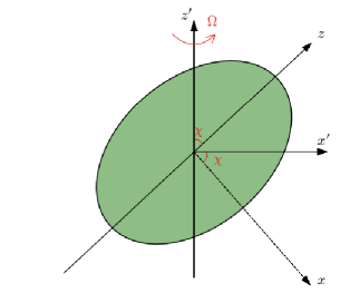
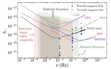
Figure 7: Left panel: Schematic diagram of a B-WD with $z^{\prime}$ being the rotational axis and $z$ as the magnetic axis. Right panel: The dimensionless GW amplitudes for WDs are shown as functions of frequency, along with the sensitivity curves of various detectors. Optimum $i$ is chosen for $\chi$ at $t=0$. See Kalita2020 .

Since a pulsating WD can emit both dipole and GW radiations simultaneously, it is associated with both dipole and quadrupolar luminosities. Dipole luminosity for an axisymmetric WD is Melatos2000

$$L_{D}=\frac{B_{p}^{2}R_{p}^{6}\Omega^{4}}{2c^{3}}{\rm sin}^{2}\,\chi\,F(x_{0}),$$ (23)

where $x_{0}=R_{0}\Omega/c$, $B_{p}$ is the magnetic field strength at the pole, $R_{p}$ is the radius of the pole and $R_{0}$ is the average WD radius. The function $F(x_{0})$ is defined as

$$F(x_{0})=\frac{x_{0}^{4}}{5(x_{0}^{6}-3x_{0}^{4}+36)}+\frac{1}{3(x_{0}^{2}+1)}.$$ (24)

Similarly, the quadrupolar GW luminosity is given by ZS1979

$$L_{GW}=\frac{2G}{5c^{5}}(I_{zz}-I_{xx})^{2}\Omega^{6}{\rm sin}^{2}\,\chi\,(1+15{\rm sin}^{2}\,\chi).$$ (25)

It should be noted that this formula is valid if $\chi$ is very small. The total luminosity is due to both dipole and gravitational radiations. Therefore, $\Omega$ and $\chi$ decay with time due to both $L_{D}$ and $L_{GW}$, given by Melatos2000

$$\frac{d(\Omega I_{z^{\prime}z^{\prime}})}{dt}=-\frac{2G}{5c^{5}}(I_{zz}-I_{xx})^{2}\Omega^{5}{\rm sin}^{2}\,\chi\,(1+15\,{\rm sin}^{2}\,\chi)-\frac{B_{p}^{2}R_{p}^{6}\Omega^{3}}{2c^{3}}{\rm sin}^{2}\,\chi\,F(x_{0}),$$

(26)

$$I_{z^{\prime}z^{\prime}}\frac{d\chi}{dt}=-\frac{12G}{5c^{5}}(I_{zz}-I_{xx})^{2}\Omega^{4}{\rm sin}^{3}\,\chi\,{\rm cos}\,\chi-\frac{B_{p}^{2}R_{p}^{6}\Omega^{2}}{2c^{3}}{\rm sin}\,\chi\,{\rm cos}\,\chi\,F(x_{0}),$$

where $I_{z^{\prime}z^{\prime}}$ is the moment of inertia about the $z^{\prime}$-axis. Equations (26) and (27) need to be solved simultaneously to obtain the timescale over which a WD can radiate.

The right panel of Figure 7 shows the dimensionless GW amplitudes for WDs as functions of their frequencies, along with the sensitivity curves of various detectors. We find that the isolated WDs may not be detected directly by LISA but can be detected after integrating the signal-to-noise ratio (SNR) for 1 year. As WDs are larger in size compared to NS, they cannot rotate as fast as NS and hence ground-based GW detectors such as LIGO, Virgo and KAGRA are not expected to detect the isolated WDs. These isolated WDs are also free from the noise due to the galactic binaries as well as from the extreme mass ratio inspirals (EMRIs).

A pulsar-like object radiates GWs at two frequencies. When we observe such a GW signal whose strength remains unchanged during the observation time $T$, the corresponding detector’s cumulative SNR is given by Jara1998 ; Bennett2010

$${\rm SNR}=\sqrt{S/N_{\Omega}^{2}+S/N_{2\Omega}^{2}}$$ (28)

where

$$\langle S/N_{\Omega}^{2}\rangle=\frac{{\rm sin}^{2}\zeta}{100}\frac{h_{0}^{2}T{\rm sin}^{2}2\chi}{S_{n}(f)},\langle S/N_{2\Omega}^{2}\rangle=\frac{4{\rm sin}^{2}\zeta}{25}\frac{h_{0}^{2}T{\rm sin}^{4}\chi}{S_{n}(2f)}$$ (29)

where $\zeta$ is the angle between the interferometer arms and $S_{n}(f)$ is the detector’s power spectral density (PSD) at the frequency $f$ with $\Omega=2\pi f$. As we mostly deal with space-based interferometers such as LISA, we assume $\zeta=60^{\circ}$. The average is over all possible angles, including $i$, which determine the object’s orientation with respect to the celestial sphere reference frame.

Figure 8 shows the SNR as a function of time for toroidal field-dominated WDs with different field strengths. We assume that these toroidal-dominated WDs have a poloidal surface field which is nearly four orders of magnitude smaller than the maximum toroidal field $B_{\rm max}$ inside the WD. Of course, such a poloidal field cannot change the shape and size of the WD, as does the toroidal field. The surface field strength is relatively very small (as is the dipole luminosity), and so it hardly changes $\Omega$ and $\chi$ within a 1 yr period. The left panel of Figure 8 shows the SNR for a B-WD with $B_{\rm max}=2.6\times 10^{14}\,{\rm G}$ with mass $1.7M_{\odot}$. All the GW detectors except LISA can easily detect such a WD almost immediately, and LISA can detect it in 5 months of integration. In contrast, when the field strength decreases ($B_{\rm max}\approx 10^{14}\,{\rm G}$) the SNR decreases, and LISA and TianQin can no longer detect them, as shown in the right panel. However, they can still be detected by ALIA, BBO and DECIGO within 1 yr of integration time.

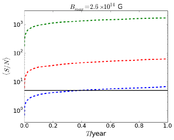
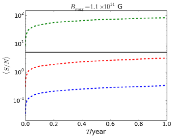
Figure 8: SNR as a function of integration time for a toroidal field-dominated WD with central density $\rho_{c}=2\times 10^{10}\,{\rm g\ cm^{-3}}$, spin period $P=2\,{\rm s}$, $\chi=30^{\circ}$ and $d=100\,{\rm pc}$. The green (top) line represents ALIA, the red (middle) line represents TianQin and blue (bottom) line represents LISA. The solid black line corresponds to $\langle S/N\rangle\approx 5$. See Kalita2021 .

Figure 9 shows the SNR as a function of integration time for XTE J1810-197, assuming $\chi=45^{\circ}$. We choose the maximum radius of this source to be 3000 km instead of 4000 km if it is a WD because its spin is fast and the XNS code does not run for 4000 km with such high rotation frequency. The left panel of Figure 9 shows that BBO and DECIGO would be able to detect it within 20 d and 100 d, respectively, if it is a 3000 km poloidal field-dominated WD. If it is a toroidally dominated WD, BBO and DECIGO could immediately detect it, and ALIA would be able to detect it within 5 months only if it is a 3000 km toroidally dominated WD (see right panel).

There are many other plausible detectabilities, e.g., via their activity in binary systems, which will be explored in the future.

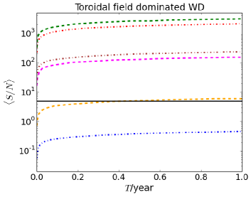
Figure 9: SNR as a function of integration time for XTE J1810-197 assuming $\chi=45^{\circ}$. The first, second and fifth lines from top correspond to a WD with radius 3000 km for BBO, DECIGO and ALIA respectively, while third, fourth and sixth lines from top represent a WD with radius 1000 km for BBO, DECIGO and ALIA respectively. The solid black line corresponds to $\langle S/N\rangle\approx 5$. See Kalita2021 .

8 Matter Anisotropy Effects in Highly Magnetised White Dwarfs

It has been shown that the presence of a strong magnetic field, the anisotropy of dense matter, and the orientation of a magnetic field can significantly influence the properties of neutron and quark stars Deb2021 . The stability of them and B-WDs is not achieved unless one considers the anisotropy of the system arising from the combined effects of Deb2021 ; Deb2022 : (i) anisotropy due to strong magnetic fields and (ii) anisotropy of the system fluid.

The effective contributions from the matter and magnetic field lead to the system density given by

$$\tilde{\rho}=\rho+\frac{B^{2}}{8\pi}.$$ (30)

The system pressure along the direction of magnetic field is represented as parallel pressure and takes the form based on magnetic field orientations as

$$p_{||}=\begin{cases}p_{r}-\frac{B^{2}}{8\pi},{\rm\ for\ radial\ orientation}\\ p_{t}-\frac{B^{2}}{8\pi},{\rm\ for\ transverse\ orientation}.\end{cases}$$ (31)

Similarly, the system pressure that aligns perpendicular to the magnetic fields is defined as transverse pressure and is based on the magnetic field orientations

$$p_{\perp}=\begin{cases}p_{t}+\frac{B^{2}}{8\pi},{\rm\ for\ radial\ orientation}\\ p_{r}+\frac{B^{2}}{8\pi},{\rm\ for\ transverse\ orientation}.\end{cases}$$ (32)

The essential magnetostatic stellar equations which describe static, spherically symmetric B-WDs are

$$\frac{dm}{dr}=4\pi\left(\rho+\frac{B^{2}}{8\pi}\right)r^{2},$$ (33)

and for radial orientation (RO)

$$\frac{dp_{r}}{dr}=\frac{-(\rho+p_{r})\frac{4\pi r^{3}\left(p_{r}-\frac{B^{2}}{8\pi}\right)+m}{r(r-2m)}+\frac{2}{r}\Delta}{\left[1-\frac{d}{d\rho}\left(\frac{B^{2}}{8\pi}\right)\frac{d\rho}{dp_{r}}\right]},$$ (34)

whereas for transverse orientation (TO)

$$\frac{dp_{r}}{dr}=\frac{-\left(\rho+p_{r}+\frac{B^{2}}{4\pi}\right)\frac{4\pi r^{3}\left(p_{r}+\frac{B^{2}}{8\pi}\right)+m}{r(r-2m)}+\frac{2}{r}\Delta}{\left[1+\frac{d}{d\rho}\left(\frac{B^{2}}{8\pi}\right)\frac{d\rho}{dp_{r}}\right]}.$$ (35)

We describe the effective anisotropy of the stars with $\Delta$, which depends on the magnetic field orientations given by $p_{t}-p_{r}+\frac{B^{2}}{4\pi}$ in case of RO and $p_{t}-p_{r}-\frac{B^{2}}{4\pi}$ for TO. We have for RO

$$\Delta=\kappa\frac{(\rho+\rho_{r})\left(\rho+3p_{r}-\frac{B^{2}}{4\pi}\right)}{\left(1-\frac{2m}{r}\right)}r^{2},$$ (36)

and for TO

$$\Delta=\kappa\frac{(\rho+\rho_{r}+\frac{B^{2}}{4\pi})\left(\rho+3p_{r}+\frac{B^{2}}{2\pi}\right)}{\left(1-\frac{2m}{r}\right)}r^{2},$$ (37)

where $\kappa$ is a dimensionless constant that describes the strength of anisotropy within the stellar structure. Note that $\kappa=0$ implies the anisotropy effects that arise due to matter properties and magnetic field both vanish. However, the case of $B=0$ but $\kappa\neq 0$ implies that only the anisotropy due to magnetic field vanishes. We have shown that highly magnetized WD models, which do not account for the combined anisotropic effects of the fluid and field, are eliminated, as they suffer from an instability at the stellar center.

To solve the magneto-hydrostatic stellar structure equations from the stellar center to surface, it is needed to supply an EoS along with a functional form of $\Delta$. Here, we consider the EoS proposed by Chandrasekhar to describe degenrate electrons of WDs as

$$p_{r}=\frac{\pi m_{e}^{4}c^{5}}{3h^{3}}\left[x(2x^{2}-3)\sqrt{x^{2}+1}+3{\rm sinh}^{-1}x\right],\ \rho=\frac{8\pi\mu_{e}m_{H}(m_{e}c)^{3}}{3h^{3}}x^{3},$$ (38)

where $m_{e}$ is the mass of an electron, $m_{H}$ is the mass of a hydrogen atom, $h$ is Planck’s constant, $\mu_{e}$ is the mean molecular weight per electron, and $x=p_{F}/m_{e}c$ with $p_{F}$ is the Fermi momentum. For the carbon-oxygen WDs, $\mu_{e}=2$.

We show the mass-radius relations of B-WDs for different $B_{0}$, $\kappa$ and $\gamma$ in Figure 10. For TO fields with $B_{0}=3.79\times 10^{14}\,{\rm G}$, a maximum mass B-WD of $2.8M_{\odot}$ is obtained, whose radius is 1457.67 km. For an RO field with $B_{0}=1.2\times 10^{14}\,{\rm G}$, the maximum mass drops to $1.62M_{\odot}$, and the radius of the B-WD is 454.67 km. For $B_{0,TO}=3.79\times 10^{14}\,{\rm G}$, the maximum mass and the corresponding radius of B-WDs increase by $\sim 70\%$ and $\sim 57\%$, respectively, compared to the non-magnetized but anisotropic case. For $B_{0,RO}=1.2\times 10^{14}\,{\rm G}$, the maximum mass and the corresponding radius decrease by $\sim 2\%$ and $\sim 52\%$, respectively, compared to the values of non-magnetized but anisotropic WDs. Even without considering the magnetic field and incorporating the effects of local anisotropy due to the fluid, it is possible to push the maximum mass of WDs beyond the Chandrasekhar mass limit. For example, by considering $\kappa=2/3$, we obtain a maximum mass for a non-magnetized but anisotropic WD of $1.81M_{\odot}$. The corresponding radius is 956.08 km. These values are $\sim 29\%$ and $\sim 8\%$, respectively, higher than the respective values of WDs at the Chandrasekhar mass limit. Moreover, with increasing $\eta$ and $\gamma$ for the TO field case, the mass of anisotropic B-WDs changes significantly, as can be seen in the right panel of Figure 10. It shows that the maximum mass of a B-WD with $\gamma=0.9$ and $\eta=0.2$ increases by $\sim 46\%$ compared to $\gamma=0.6$ and $\eta=0.1$.

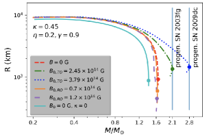
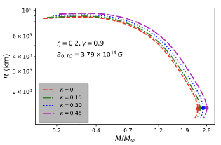
(a)	(b)	(c)

Figure 10: Stellar radius ($R$) as a function of gravitational mass ($M/M_{\odot}$) for different (a) $B_{0}$ (left panel), (b) $\kappa$ (middle panel), and (c) $\eta$ and $\gamma$ (right panel). Solid circles represent the stars with the maximum-possible masses. See Deb2022 .

For RO fields, we can explain sub-, standard- and super-Chandrasekhar B-WDs by making appropriate choices of $B_{0,RO}$ and $\kappa$ (see Figure 11). By changing both $B_{0,RO}$ and $\kappa$, as shown in the left panel of Figure 11, we successfully explain both (i) the sub- and standard-Chandrasekhar progenitor B-WDs and (ii) the standard and super-Chandrasekhar progenitor B-WDs by a single mass-radius curve for the respective cases. On the other hand, through changes of only $B_{0,RO}$ or $\kappa$, sub-, standard- and super-Chandrasekhar B-WDs line up in a series of mass-radius curves; see, e.g., the middle and right panels of Figure 11. This leads to a complete explanation of under-, regular- and over-luminous SNeIa in a single theory.

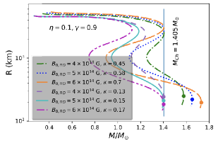
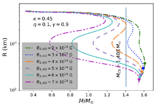
(a)	(b)	(c)

Figure 11: Stellar radius ($R$) as a function of gravitational mass ($M/M_{\odot}$) for varying (a) $B_{0,RO}$ and $\kappa$ (left panel), (b) $B_{0,RO}$ (middle panel), and (c) $\kappa$ (right panel). Solid circles represent the stars with the maximum possible masses. See Deb2022 .

9 Conclusions

Reviewing the work in last decade or so, we have confirmed that, at least theoretically, massive NSs and WDs, heavier than their conventional counterparts as observed/inferred from recent data, are possibly highly magnetized, rotating stable compact stars. They have multiple implications including enigmatic peculiar over-luminous SNeIa. Numerical simulations based on Cambridge stellar evolution code STARS argue B-WDs to be toroidally (centrally) dominated with lower, maybe dipole, surface magnetic fields. The new generic mass-limit of WDs seems to be well above $2M_{\odot}$, around $2.8M_{\odot}$, depending on the magnetic field profile/geometry and rotational frequency.

However, these massive compact objects, particularly WDs, have hardly been observed directly due to their apparently very low luminosity. On the other hand, the presence of magnetic fields and rotation by definition brings in anisotropy in these compact objects, leading them to be triaxial when the magnetic and rotation axes are misaligned. Therefore, they are expected to emit continuous GW. Hence, B-WDs can be detected directly by the missions LISA (in one year integration time), DECIGO/BBO and the magnetised NSs can be detected by aLIGO, aVIRGO, Einstein Telescope.

Nevertheless, the magnetic fields therein start decaying beyond million years, hence these massive compact objects may not survive beyond this time. Moreover, due to their electromagnetic and gravitational radiation, the angular velocity and the misalignment angle between magnetic and rotation axes decrease, leading them to lose their pulsar nature and detection possibility. This is another reason why they are so rare and/or hard to detect unless targeted at an appropriate time. Therefore, appropriate missions in GW astronomy and otherwise, e.g., radio astronomy, should be planned to probe them.

Both the authors share an equal authorship. However, various figures presented in this manuscript are based on previous works by B.M. and his collaborators. The work was conceptualized by B.M.; the methodology was initiated by B.M. and further was carried out by B.M. and M.B.; investigation was initiated by B.M. and was further taken over by M.B.; the first draft was prepared by M.B. and further was revised and edited by B.M. and M.B.

M.B. would like to acknowledge support from the Eberly Research Fellowship at the Pennsylvania State University.

- (1) Abbott, R.; Abbott T.D.; Abraham, S.; Acernese, F.; Ackley, K.; Adams, C.; Adhikari, R.X.; Adya, V.B.; Affeldt, C.; Agathos, M.; et al. GW190814: Gravitational Waves from the Coalescence of a 23 Solar Mass Black Hole with a 2.6 Solar Mass Compact Object. Astrophys. J. Lett. 2020, 896, L44. http://doi.org/10.3847/2041-8213/ab960f.
- (2) MacFadyen, A.I.; Woosley, S.E. Collapsars: Gamma-Ray Bursts and Explosions in “Failed Supernovae”. Astrophys. J. 1999, 524, 262. http://doi.org/10.1086/307790.
- (3) Pooley, D.; Kumar, P.; Wheeler, J.; Grossan, B. GW170817 Most Likely Made a Black Hole. Astrophys. J. Lett. 2018, 859, L23. http://doi.org/10.3847/2041-8213/aac3d6.
- (4) Ozel, F.; Psaltis, D.; Narayan, R.; McClintock, J.E. The Black Hole Mass Distribution in the Galaxy. Astrophys. J. 2010, 725, 1918. http://doi.org/10.1088/0004-637X/725/2/1918.
- (5) Alsing, J.; O’Silva, H.; Berti, E. Evidence for a maximum mass cut-off in the neutron star mass distribution and constraints on the equation of state. Mon. Not. R. Astron. Soc. 2018, 478, 1377. http://doi.org/10.1093/mnras/sty1065.
- (6) Cromartie, H.T.; Fonseca, E.; Ransom, S.M.; Demorest, P.B.; Arzoumanian, Z.; Blumer, H.; Brook, P.R.; DeCesar, M.E.; Dolch, T.; Ellis, J.A.; et al. Relativistic Shapiro delay measurements of an extremely massive millisecond pulsar. Nat. Astron. 2020, 4, 72–76. http://doi.org/10.1038/s41550-019-0880-2.
- (7) Zhang, C.M.; Wang, J.; Zhao, Y.H.; Yin, H.X.; Song, L.M.; Menezes, D.P.; Wickramasinghe, D.T.; Ferrario, L.; Chardonnet, P. Study of measured pulsar masses and their possible conclusions. Astron. Astrophys. 2011, 527, A83. http://doi.org/10.1051/0004-6361/201015532.
- (8) Miller, M.C. Astrophysical Constraints on Dense Matter in Neutron Stars. In Timing Neutron Stars: Pulsations, Oscillations and Explosions; Astrophysics and Space Science Library (ASSL); Springer: Berlin/Heidelberg, Germany, 2021; Volume 461. http://doi.org/10.1007/978-3-662-62110-3_1.
- (9) Khokhlov, A. M. Delayed detonation model for type Ia supernovae. Astron. Astrophys. 1991, 245, 114–128.
- (10) Scalzo, R.A.; Aldering, G.; Antilogus, P.; Aragon, C.; Bailey, S.; Baltay, C.; Bongard, S.; Buton, C.; Childress, M.; Chotard, N.; et al. Nearby Supernova Factory Observations of SN 2007if: First Total Mass Measurement of a Super-Chandrasekhar-Mass Progenitor. Astrophys. J. 2010, 713, 1073–1094. http://doi.org/10.1088/0004-637X/713/2/1073.
- (11) Howell, D.A.; Sullivan, M.; Nugent, P.E.; Ellis, R.S.; Conley, A.J.; Le Borgne, D.; Carlberg, R.G.; Guy, J.; Balam, D.; Basa, S.; et al. Carlberg, R.G.; Guy, J.; Balam, D.; Basa, S.; The type Ia supernova SNLS-03D3bb from a super-Chandrasekhar-mass white dwarf star. Nature 2006, 443, 7109, 308–311. http://doi.org/10.1038/nature05103.
- (12) Das, U.; Mukhopadhyay, B. Strongly magnetized cold degenerate electron gas: Mass-radius relation of the magnetized white dwarf. Phys. Rev. D 2012, 86, 042001. http://doi.org/10.1103/PhysRevD.86.042001.
- (13) Das, U.; Mukhopadhyay, B. New Mass Limit for White Dwarfs: Super-Chandrasekhar Type Ia Supernova as a New Standard Candle. Phys. Rev. Lett. 2013, 110, 071102. http://doi.org/10.1103/PhysRevLett.110.071102.
- (14) Das, U.; Mukhopadhyay, B.; Rao, A. R. A Possible Evolutionary Scenario of Highly Magnetized Super-Chandrasekhar White Dwarfs: Progenitors of Peculiar Type Ia Supernovae Astrophys. J. Lett. 2013, 767, L14. http://doi.org/10.1088/2041-8205/767/1/L14.
- (15) Das, U.; Mukhopadhyay, B. Maximum mass of stable magnetized highly super-Chandrasekhar white dwarfs: Stable solutions with varying magnetic fields. J. Cosmol. Astropart. Phys. 2014, 06, 050. http://doi.org/10.1088/1475-7516/2014/06/050.
- (16) Das, U.; Mukhopadhyay, B. GRMHD formulation of highly super-Chandrasekhar magnetized white dwarfs: Stable configurations of non-spherical white dwarfs. J. Cosmol. Astropart. Phys. 2015, 05, 016. http://doi.org/10.1088/1475-7516/2015/05/016.
- (17) Subramanian, S.; Mukhopadhyay, B. GRMHD formulation of highly super-Chandrasekhar rotating magnetized white dwarfs: Stable configurations of non-spherical white dwarfs. Mon. Not. R. Astron. Soc. 2015, 454, 1, 752–765. http://doi.org/10.1093/mnras/stv1983.
- (18) Bhattacharya, M.; Mukhopadhyay, B.; Mukerjee, S. Luminosity and cooling of highly magnetized white dwarfs: Suppression of luminosity by strong magnetic fields. Mon. Not. R. Astron. Soc. 2018, 477, 2705–2715. http://doi.org/10.1093/mnras/sty776.
- (19) Bhattacharya, M.; Mukhopadhyay, B.; Mukerjee, S. Luminosity and cooling suppression in magnetized white dwarfs. arXiv 2018, arXiv:1810.07836.
- (20) Gupta, A.; Mukhopadhyay, B.; Tout, C.A. Suppression of luminosity and mass-radius relation of highly magnetized white dwarfs. Mon. Not. R. Astron. Soc. 2020, 496, 894–902. http://doi.org/10.1093/mnras/staa1575.
- (21) Mukhopadhyay, B.; Bhattacharya, M.; Hackett, A.J.; Kalita, S.; Karinkuzhi, D.; Tout, C.A. Highly magnetized white dwarfs: Implications and current status. arXiv 2021, arXiv:2110.15374.
- (22) Bhattacharya, M.; Hackett, A.J.; Gupta, A.; Tout, C.A.; Mukhopadhyay, B. Evolution of Highly Magnetic White Dwarfs by Field Decay and Cooling: Theory and Simulations. Astrophys. J. 2022, 925, 133. http://doi.org/10.3847/1538-4357/ac450b.
- (23) Banerjee, S.; Shankar, S.; Singh, T.P. Constraints on modified gravity models from white dwarfs. J. Cosmol. Astropart. Phys. 2017, 2017, 004. http://doi.org/10.1088/1475-7516/2017/10/004.
- (24) Eslam Panah, B.E.; Liu, H. White dwarfs in de Rham-Gabadadze-Tolley like massive gravity. Phys. Rev. D 2019, 99, 104074. http://doi.org/10.1103/PhysRevD.99.10407.
- (25) Kalita, S.; Mukhopadhyay, B.; Govindarajan, T.R. Significantly super-Chandrasekhar mass-limit of white dwarfs in noncommutative geometry. Int. J. Mod. Phys. D 2021, 30, 2150034. http://doi.org/10.1142/S0218271821500346.
- (26) Kalita, S.; Mukhopadhyay, B.; Govindarajan, T.R. Super-Chandrasekhar limiting mass white dwarfs as emergent phenomena of noncommutative squashed fuzzy spheres. Int. J. Mod. Phys. D 2021, 30, 2150101. http://doi.org/10.1142/S0218271821501017.
- (27) Bertolami, O.; Mariji, H. White dwarfs in an ungravity-inspired model. Phys. Rev. D 2016, 93, 104046.http://doi.org/10.1103/PhysRevD.93.104046.
- (28) Liu, H.; Zhang, X.; Wen. D. One possible solution of peculiar type Ia supernovae explosions caused by a charged white dwarf. Phys. Rev. D 2014, 89, 104043. http://doi.org/10.1103/PhysRevD.89.104043.
- (29) Carvalho, G.A.; Arbanil, Jose D.V.; Marinho, R.M.; Malheiro, M. White dwarfs with a surface electrical charge distribution: Equilibrium and stability. Eur. Phys. J. C 2018, 78, 411. http://doi.org/10.1140/epjc/s10052-018-5901-2.
- (30) Belyaev, V.B.; Ricci, P.; Simkovic, F.; Adam, J.; Tater, M.; Truhlik, E. Consequence of total lepton number violation in strongly magnetized iron white dwarfs. Nucl. Phys. A 2015, 937, 17–43. http://doi.org/10.1016/j.nuclphysa.2015.02.002.
- (31) Herrera, L.; Barreto, W. Newtonian polytropes for anisotropic matter: General framework and applications. Phys. Rev. D 2013, 87, 087303. http://doi.org/10.1103/PhysRevD.87.087303.
- (32) Glendenning, N.K. Compact Stars. Nuclear Physics, Particle Physics and General Relativity; Springe: New York, NY, USA, 1996.
- (33) Chanmugam, G. Magnetic fields of degenerate stars. Annu. Rev. Astron. Astrophys. 1992, 30, 143–184. http://doi.org/10.1146/annurev.aa.30.090192.001043.
- (34) Ferrario, L.; Wickramasinghe, D.T. Magnetic fields and rotation in white dwarfs and neutron stars. Mon. Not. R. Astron. Soc. 2005, 356, 615–620, http://doi.org/10.1111/j.1365-2966.2004.08474.x.
- (35) Ferrario, L.; Wickramasinghe, D.T.; Kawka, A. Magnetic fields in isolated and interacting white dwarfs. Adv. Space Res. 2020, 66, 1025–1056. http://doi.org/10.1016/j.asr.2019.11.012.
- (36) Wickramasinghe, D.T.; Ferrario, L. Magnetism in Isolated and Binary White Dwarfs. Publ. Astron. Soc. Pac. 2000, 112, 873–924. http://doi.org/10.1086/316593.
- (37) Cumming, A. Magnetic field evolution in accreting white dwarfs. Mon. Not. R. Astron. Soc. 2002, 333, 589–602. http://doi.org/10.1046/j.1365-8711.2002.05434.x.
- (38) Zhang, C.M.; Wickramasinghe, D.T.; Ferrario, L. Is there evidence for field restructuring or decay in accreting magnetic white dwarfs?. Mon. Not. R. Astron. Soc. 2009, 397, 2208–2215. http://doi.org/10.1111/j.1365-2966.2009.15154.x.
- (39) Mukhopadhyay, B.; Rao, A.R. Soft gamma-ray repeaters and anomalous X-ray pulsars as highly magnetized white dwarfs. J. Cosmol. Astropart. Phys. 2016, 05, 007. http://doi.org/10.1088/1475-7516/2016/05/007.
- (40) Mukhopadhyay, B.; Das, U.; Rao, A.R.; Subramanian, S.; Bhattacharya, M.; Mukerjee, S.; Bhatia, T.S.; Sutradhar, J. Significantly Super-Chandrasekhar Limiting Mass White Dwarfs and their Consequences. arXiv 2016, arXiv:1611.00133.
- (41) Mukhopadhyay, B.; Bhattacharya, M.; Rao, A.R.; Mukerjee, S.; Das, U. Possible formation of lowly luminous highly magnetized white dwarfs by accretion leading to SGRs/AXPs. arXiv 2019, arXiv:1908.10045.
- (42) Kalita, S.; Mukhopadhyay, B. Continuous gravitational wave from magnetized white dwarfs and neutron stars: Possible missions for LISA, DECIGO, BBO, ET detectors. Mon. Not. R. Astron. Soc. 2019, 490, 2692–2705. http://doi.org/10.1093/mnras/stz2734.
- (43) Kalita, S.; Mukhopadhyay, B.; Mondal, T.; Bulik, T. Timescales for Detection of Super-Chandrasekhar White Dwarfs by Gravitational-wave Astronomy. Astrophys. J. 2020, 896, 69. http://doi.org/10.3847/1538-4357/ab8e40.
- (44) Kalita, S.; Mondal, T.; Tout, C. A.; Bulik, T.; Mukhopadhyay, B. Resolving dichotomy in compact objects through continuous gravitational waves observation. Mon. Not. R. Astron. Soc. 2021, 508, 1, 842–851. http://doi.org/10.1093/mnras/stab2625.
- (45) Vanlandingham, K.; Schmidt, G.; Eisenstein, D.; Harris, H.C.; Anderson, S.F.; Hall, P.B.; Liebert, J.; Schneider, D.P.; Silvestri, N.M.; Stinson, G.S.; et al. Magnetic White Dwarfs from the SDSS. II. The Second and Third Data Releases. Astron. J. 2005, 130, 734–741. http://doi.org/10.1086/431580.
- (46) Ferrario, L.; de Martino, D.; Gänsicke, B.T. Magnetic White Dwarfs. Space Sci. Rev. 2015, 191, 111–169. http://doi.org/10.1007/s11214-015-0152-0.
- (47) Boshkayev, K.; Rueda, J.; Ruffini, R.; Siutsou, I. On General Relativistic Uniformly Rotating White Dwarfs. Astrophys. J. 2013, 762, 117. http://doi.org/10.1088/0004-637X/762/2/117.
- (48) Franzon, B.; Schramm, S. Effects of strong magnetic fields and rotation on white dwarf structure. Phys. Rev. D 2015, 92, 083006. http://doi.org/10.1103/PhysRevD.92.083006.
- (49) Ablimit, I.; Maeda, K. Evolution of Magnetized White Dwarf Binaries to Type Ia Supernovae. Astrophys. J. 2019, 871, 31. http://doi.org/10.3847/1538-4357/aaf722.
- (50) Ablimit, I.; Maeda, K. Possible Contribution of Magnetized White Dwarf Binaries to Type Ia Supernova Populations. Astrophys. J. 2019, 885, 99. http://doi.org/10.3847/1538-4357/ab4814.
- (51) Ablimit, I. The magnetized white dwarf + helium star binary evolution with accretion-induced collapse. Mon. Not. R. Astron. Soc. 2022, 509, 6061. http://doi.org/10.1093/mnras/stab3060.
- (52) Ablimit, I. The CO White Dwarf + Intermediate-mass/Massive Star Binary Evolution: Possible Merger Origins for Peculiar Type Ia and II Supernovae. Publ. Astron. Soc. Pac. 2021, 133, 074201. http://doi.org/10.1088/1538-3873/ac025c.
- (53) Markey, P.; Tayler, R.J. The adiabatic stability of stars containing magnetic fields. II. Poloidal fields. Mon. Not. R. Astron. Soc. 1973, 163, 77–91. https://doi.org/10.1093/mnras/163.1.77.
- (54) Tayler, R.J. The adiabatic stability of stars containing magnetic fields. I: Toroidal fields. Mon. Not. R. Astron. Soc. 1973, 161, 365–380. http://doi.org/10.1093/mnras/161.4.365.
- (55) Wickramasinghe, D.T.; Tout, C.A.; Ferrario, L. The most magnetic stars. Mon. Not. R. Astron. Soc. 2014, 437, 675–681. http://doi.org/10.1093/mnras/stt1910.
- (56) Quentin, L.G.; Tout, C.A. Rotation and magnetism in intermediate-mass stars. Mon. Not. R. Astron. Soc. 2018, 477, 2298–2309. http://doi.org/10.1093/mnras/sty770.
- (57) Mukhopadhyay, B.; Rao, A.R.; Bhatia, T.S. AR Sco as a possible seed of highly magnetized white dwarf. Mon. Not. R. Astron. Soc. 2017, 472, 3564–3569. http://doi.org/10.1093/mnras/stx2119.
- (58) Mukhopadhyay, B.; Sarkar, A.; Tout, C.A. Modified virial theorem for highly magnetized white dwarfs. Mon. Not. R. Astron. Soc. 2021, 500, 763–771. http://doi.org/10.1093/mnras/staa3136.
- (59) Pili, A.G.; Bucciantini, N.; Del Zanna, L. Axisymmetric equilibrium models for magnetized neutron stars in General Relativity under the Conformally Flat Condition. Mon. Not. R. Astron. Soc. 2014, 439, 3541–3563. http://doi.org/10.1093/mnras/stu215.
- (60) Ioka, K.; Sasaki, M. Relativistic Stars with Poloidal and Toroidal Magnetic Fields and Meridional Flow. Astrophys. J. 2004, 600, 296–316. http://doi.org/10.1086/379650.
- (61) Frieben, J.; Rezzolla, L. Equilibrium models of relativistic stars with a toroidal magnetic field. Mon. Not. R. Astron. Soc. 2012, 427, 3406–3426. http://doi.org/10.1111/j.1365-2966.2012.22027.x
- (62) Chandrasekhar, S.; Fermi, E. Problems of Gravitational Stability in the Presence of a Magnetic Field. Astrophys. J. 1953, 118, 116. http://doi.org/10.1086/145732.
- (63) Komatsu, H.; Eriguchi, Y.; Hachisu, I. Rapidly rotating general relativistic stars. I - Numerical method and its application to uniformly rotating polytropes. Mon. Not. R. Astron. Soc. 1989, 237, 355–379. http://doi.org/10.1093/mnras/237.2.355.
- (64) Braithwaite, J. Axisymmetric magnetic fields in stars: Relative strengths of poloidal and toroidal components. Mon. Not. R. Astron. Soc. 2009, 397, 763–774. http://doi.org/10.1111/j.1365-2966.2008.14034.x.
- (65) Heyl, J.S. Gravitational radiation from strongly magnetized white dwarfs. Mon. Not. R. Astron. Soc. 2000, 317, 310–314. http://doi.org/10.1046/j.1365-8711.2000.03533.x.
- (66) Brinkworth, C.; Burleigh, M.; Lawrie, K.; Marsh, T.R.; Knigge, C. Measuring the Rotational Periods of Isolated Magnetic White Dwarfs. Astrophys. J. 2013, 773, 47. http://doi.org/10.1088/0004-637X/773/1/47.
- (67) Shah, H.; Sebastian, K. Central Magnetic Field of a Magnetic White Dwarf Star. Astrophys. J. 2017, 843, 131. http://doi.org/10.3847/1538-4357/aa74dd.
- (68) Stergioulas, N. Rotating Stars in Relativity. Living Rev. Relativ. 2003, 6, 3. http://doi.org/10.12942/lrr-2003-3.
- (69) Bucciantini, N.; Del Zanna, L. General relativistic magnetohydrodynamics in axisymmetric dynamical spacetimes: The X-ECHO code. Astron. Astrophys. 2011, 528, A101. http://doi.org/10.1051/0004-6361/201015945.
- (70) Sinha, M.; Mukhopadhyay, B.; Sedrakian, A. Hypernuclear matter in strong magnetic field. Nucl. Phys. A 2013, 898, 43–58. http://doi.org/10.1016/j.nuclphysa.2012.12.076.
- (71) Shapiro, S.; Teukolsky, S. Black Holes, White Dwarfs, and Neutron Stars : The Physics of Compact Objects. Wiley: New York, NY, USA, 1983.
- (72) Bandyopadhyay, D.; Chakrabarty, S.; Pal, S. Quantizing Magnetic Field and Quark-Hadron Phase Transition in a Neutron Star. Phys. Rev. Lett. 1997, 79, 2176–2179. http://doi.org/10.1016/10.1103/PhysRevLett.79.2176.
- (73) Potekhin, A.Y.; Yakovlev, D.G. Thermal structure and cooling of neutron stars with magnetized envelopes. Astron. Astrophys. 2001, 374, 213–226. http://doi.org/10.1051/0004-6361:20010698.
- (74) Ventura, J.; Potekhin, A. Neutron Star Envelopes and Thermal Radiation from the Magnetic Surface. arXiv 2001, arXiv:astro-ph/0104003.
- (75) Chandrasekhar, S. The highly collapsed configurations of a stellar mass. Mon. Not. R. Astron. Soc. 1935, 95, 207–225. http://doi.org/10.1051/10.1093/mnras/95.3.207.
- (76) Heyl, J.S.; Kulkarni, S.R. How Common Are Magnetars? The Consequences of Magnetic Field Decay. Astrophys. J. 1998, 506, L61–L64. http://doi.org/10.1086/311628.
- (77) Lai, D.; Shapiro, S.L. Cold Equation of State in a Strong Magnetic Field: Effects of Inverse beta-Decay. Astrophys. J. 1991, 383, 745. http://doi.org/10.1086/170831.
- (78) Choudhuri, A.R. Astrophysics for Physicists; Cambridge University Press: New York, NY, USA, 2010.
- (79) Bonazzola, S.; Gourgoulhon, E. Gravitational waves from pulsars: Emission by the magnetic-field-induced distortion. Astron. Astrophys. 1996, 312, 675–690, arXiv:astro-ph/9602107.
- (80) Zimmermann, M.; Szedenits, E. Gravitational waves from rotating and precessing rigid bodies: Simple models and applications to pulsars. Phys. Rev. D 1979, 20, 351–355. http://doi.org/10.1103/PhysRevD.20.351.
- (81) Melatos, A. Radiative precession of an isolated neutron star. Mon. Not. R. Astron. Soc. 2000, 313, 217–228.http://doi.org/10.1046/j.1365-8711.2000.03031.x.
- (82) Jaranowski, P.; Krolak, A.; Schutz, B.F. Data analysis of gravitational-wave signals from spinning neutron stars: The signal and its detection. Phys. Rev. D 1998, 58, 063001. http://doi.org/10.1103/PhysRevD.58.063001.
- (83) Bennett, M.F.; van Eysden, C.A.; Melatos, A. Continuous-wave gravitational radiation from pulsar glitch recovery. Mon. Not. R. Astron. Soc. 2010, 409, 1705–1718. http://doi.org/10.1111/j.1365-2966.2010.17416.x.
- (84) Deb, D.; Mukhopadhyay, B.; Weber, F. Effects of Anisotropy on Strongly Magnetized Neutron and Strange Quark Stars in General Relativity. Astrophys. J. 2021, 922, 149. http://doi.org/10.3847/1538-4357/ac222a.
- (85) Deb, D.; Mukhopadhyay, B.; Weber, F. Anisotropic Magnetized White Dwarfs: Unifying Under- and Overluminous Peculiar and Standard Type Ia Supernovae. Astrophys. J. 2022, 926, 66. http://doi.org/10.3847/1538-4357/ac410b.