Chunyu Lichunyuli@preferred.jp1 Taisuke Hashimotohashimotot@preferred.jp1 Eiichi Matsumotomatsumoto@preferred.jp1 Hiroharu Katohkato@preferred.jp1 Preferred Networks, Inc.
3F Otemachi-building,
1-6-1 Otemachi, Chiyoda-Ku,
Tokyo, Japan Multi-View Neural Surface Reconstruction

Supplementary Material to
Multi-View Neural Surface Reconstruction with Structured Light

1 Details on noise reduction

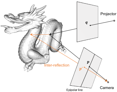
Figure 1: Illustration of pattern misdetection caused by inter-reflection.

As described in Section 2.1 of the main paper, we reduce the misdetection of the structured-light pattern caused by inter-reflection by calculating the epipolar line between the projecter and camera pair. To be specific, as shown in Fig. 1, the light projected from the projector pixel $\bm{q}$ can reach the camera in one of two general ways: (1) by direct surface reflection, captured by a camera pixel $\bm{p}$ on the epipolar line (black path), which is the desirable path of the light for pattern decoding, or (2) by inter-reflection, captured by a camera pixel $\bm{p}^{\prime}$ that is not on the epipolar line (orange path). Therefore, we can determine whether a decoded pixel is affected by inter-reflection using the epipolar line. As the camera poses are unknown in our experiment, we calculate a rough fundamental matrix between the camera and projector from the noisy corresponding points using Ransac algorithm, and estimate the epipolar lines using this fundamental matrix. Then, we eliminate correspondences whose camera pixels are not on the epipolar line. Note that although we can effectively reduce most noise using this strategy, some limitations remain: (1) the estimated epipolar lines may include minor errors owing to the noisy corresponding points, and (2) we cannot eliminate the inter-reflected correspondences whose projector and camera pixels are on corresponding epipolar lines. However, the amount of noise caused by these cases is small, so they can be further reduced by the photometric supervision introduced in Section 2.4 of the main paper. The effectiveness of this noise-reduction strategy is demonstrated by the ablation study (see Section 4.2 in supplementary material).

2 Details on triangulation

In this section we will explain the details on the calculation of $\bm{y}_{a}$ and $\bm{y}_{b}$ in Eq. (5) of the main paper. $\bm{y}_{a}$ and $\bm{y}_{b}$ are the nearest points between the two skew camera rays $R_{a}(\tau)$ and $R_{b}(\tau)$ (see the right column of Fig. 4). We denote $R_{a}(\tau)=\left\{\bm{o}_{a}+t_{a}\bm{v}_{a}\mid t_{a}\geq 0\right\}$ and $R_{b}(\tau)=\left\{\bm{o}_{b}+t_{b}\bm{v}_{b}\mid t_{b}\geq 0\right\}$. The cross product of $\bm{v}_{a}$ and $\bm{v}_{b}$ is perpendicular to the lines:

$$\bm{n}=\bm{v}_{a}\times\bm{v}_{b}.$$ (1)

The plane formed by the translations of $R_{b}(\tau)$ along $\bm{n}$ contains the point $\bm{o}_{b}$ and is perpendicular to $\bm{n}_{1}=\bm{v}_{b}\times\bm{n}$. Therefore, the intersecting point of $R_{a}(\tau)$ with the above-mentioned plane, which is also the point on $R_{b}(\tau)$ that is nearest to $R_{a}(\tau)$, is given by

$$\bm{y}_{a}=\bm{o}_{a}+\frac{(\bm{o}_{b}-\bm{o}_{a})\cdot\bm{n}_{1}}{\bm{v}_{a}\cdot\bm{n}_{1}}\bm{v}_{a}.$$ (2)

Similarly, the point on $R_{b}(\tau)$ nearest to $R_{a}(\tau)$ is given by

$$\bm{y}_{b}=\bm{o}_{b}+\frac{(\bm{o}_{a}-\bm{o}_{b})\cdot\bm{n}_{2}}{\bm{v}_{b}\cdot\bm{n}_{2}}\bm{v}_{b},$$ (3)

where $\bm{n}_{2}=\bm{v}_{a}\times\bm{n}$.

3 Initial camera poses estimation for real-world dataset

In the experiment on real-world scenes, the initial camera poses were measured using 26 AprilTag 16h5 Markers [Andrew et al.(2013)Andrew, Johannes, and Edwin] fixed on the turntable. We assume the intrinsic parameters of the cameras are known. After capturing the multi-view input images, the initial camera poses are estimated following four steps.

Step 1. Marker Detection: Given each image containing AprilTag 16h5 Markers, the detection process has to return a list of detected markers. Each detected marker includes the position of its four corners in the image and the id of the marker. This step is implemented using OpenCV ArUco module [aru()].

Step 2. Camera Pose Initialization: The next thing is to obtain the camera pose from detected markers. First, for each image, the pose of each marker in the camera coordinate system is estimated individually using OpenCV ArUco module [aru()]. Then using one marker as a reference , all camera poses in one coordinate system can be obtained by calculating the 3D transformation from each camera coordinate systems to the reference marker coordinate system.

Step 3. Camera Pose Optimization: The camera poses obtained by Step 2 usually have large error. Next they are optimized using bundle adjustment while simultaneously updating the marker poses. Specifically, our bundle adjustment jointly refining the camera poses and marker poses by minimizing the reprojection error of four corners of each marker.

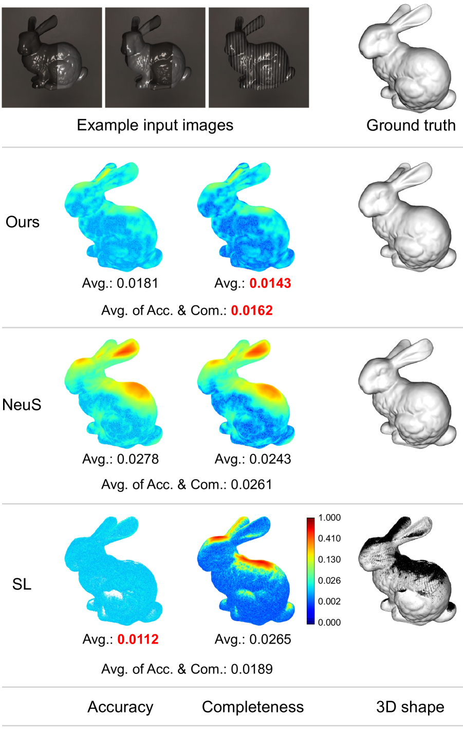
(a) Stanford Bunny (glass)

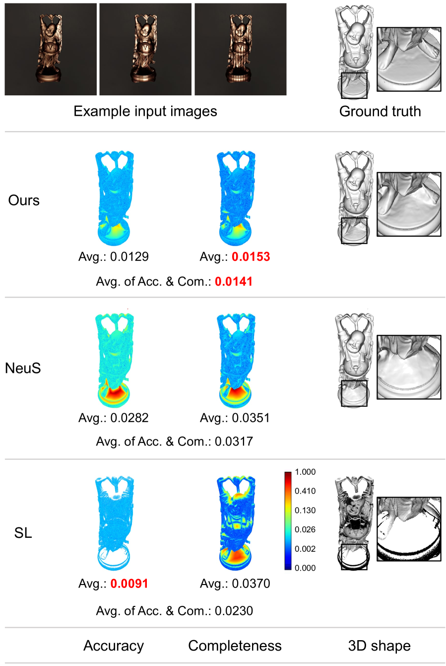
(b) Happy Buddha (metal)

Figure 2: Example input images, 3D reconstruction results, and their completeness and accuracy errors on two additional synthetic scenes with fixed ground truth camera poses.

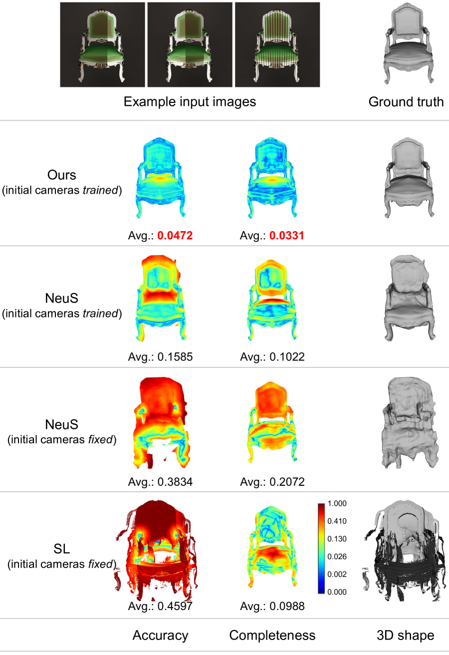
(a) Chair

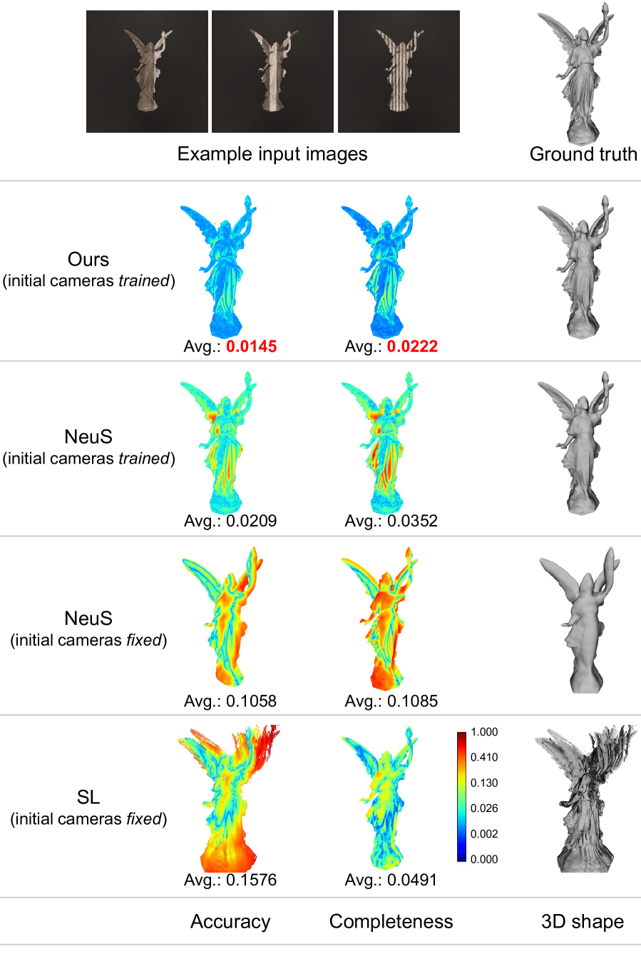
(b) Lucy (marble)

Figure 3: Example input images, 3D reconstruction results, and their completeness and accuracy errors on two additional synthetic scenes with noisy camera poses.

4 Additional experimental results

4.1 Simulation results

In this section, we show additional quantitative simulation results on a Stanford Bunny model (Fig. 2 (a)), Happy Buddha model (Fig. 2 (b)) and a Lucy model (Fig. 3 (b)) obtained from the Stanford 3D Scanning Repository [Greg and Marc()] and a Chair model with thin structure downloaded from the Internet [cha()]. To demonstrate the proposed method on the challenging targets, we rendered the models from the Stanford 3D Scanning Repository with different shiny materials, such as glass (Stanford Bunny), metal (Happy Buddha) and marble (Lucy). For each synthetic scene, the input images are generated using the same setup as described in Section 4.1 of the main paper. We used our method to generate 3D reconstructions in two different setups: (1) fixed ground-truth camera poses and (2) trainable camera poses with noisy initializations obtained using an SfM approach [Schonberger and Frahm(2016)]. Fig. 2 shows the comparisons with baseline methods with fixed ground truth camera poses. Fig. 3 shows the comparisons with baseline methods with noisy camera poses calculated by Colmap. In Table 1 we show a comparison of camera directions (Dire.) and positions (Posi.) between the noisy initial values and optimized values (Opt.). Note the considerable improvement in optimized camera accuracy over initial values.

Table 1: Camera poses accuracy w.r.t the ground truth.

	Chair		Lucy
	Initial	Opt.	Initial	Opt.
Dire.(deg)	2.832	0.177	0.781	0.106
Posi.(m)	0.119	0.037	0.830	0.044

Table 2: Quantitative results of ablation studies.

	Avg. of acc.	Avg. of comp.
(a) w/o $\mathcal{L}_{\rm SR}$	0.0101	0.0157
(b) w/o $\mathcal{L}_{\rm ST}$	0.0114	0.0160
(c) w/o noise reduction	0.0174	0.0183
(d) initial cameras fixed	0.0191	0.0194
(e) full model	0.0094	0.0155

4.2 Ablation studies

We used the glossy marble Dragon model (the same scene in Fig. 6 of the main paper) to conduct the ablation study. First, to confirm the contribution of the individual loss used for structured-light supervision (reprojection loss $\mathcal{L}_{\rm SR}$ and triangulation loss $\mathcal{L}_{\rm ST}$), we test following two cases: (a) w/o $\mathcal{L}_{\rm SR}$ (by setting $\lambda_{\rm SR}=0$), (b) w/o $\mathcal{L}_{\rm ST}$ (by setting $\lambda_{\rm ST}=0$). The quantitative results are shown in Table 2. We can confirm that the (e) full model that uses both of $\mathcal{L}_{\rm SR}$ and $\mathcal{L}_{\rm ST}$ achieves the best result. We also studied the effect of the noise reduction of decoding. The noises caused by inter-reflection leads to a deteriorated reconstruction quality as shown in Table 2 (c) when compared with the (e) full model which reduced the noises. In Table 2 (d) we show the result of training with fixed camera poses set to the inaccurate camera initializations obtain with SfM [Schonberger and Frahm(2016)]. This indicates that the joint optimization of camera poses and 3D geometry is indeed significant.

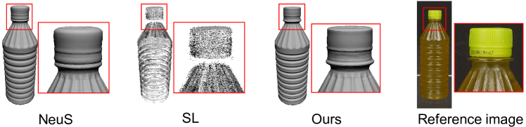
(a) Plastic bottle

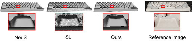
(b) Keyboard

Figure 4: Additional 3D reconstruction results on the real dataset.

4.3 Results for real-world scenes

In Fig. 4 we present additional qualitative results on the real dataset. The data acquisition follows the same setup as described in Section 4.1 of main papaer. We can confirm that proposed method perform better than all baseline methods.

4.4 Limitations

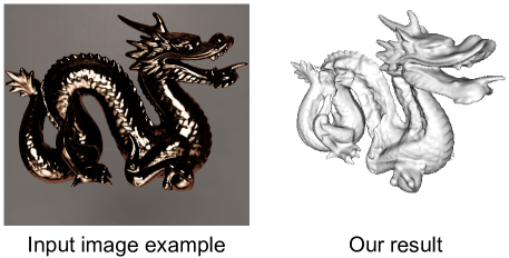
Figure 5: A failure case on a mirror-like object.

Although our method produces satisfactory results in most cases, it has several limitations. First, the projector pattern will not be captured by the cameras, and no correspondences can be obtained if the material of the object is mirror-like. In this case our method only relies on photometric supervision. In Fig. 5 we show a failure case on a synthetic scene with a textureless and mirror-like reflection. Our method fails to reconstruct an accurate surface owing to the lack of structured-light supervision. It should be noted that this material is also challenging for other state-of-the-art methods. Second, although our method can optimize camera poses, it requires a reasonable camera pose initialization using markers or SfM softwares.

References

- [aru()] Detection of ArUco Markers. https://docs.opencv.org/4.x/d5/dae/tutorial_aruco_detection.html.
- [cha()] Blend Swap. https://www.blendswap.com/blend/8261.
- [Andrew et al.(2013)Andrew, Johannes, and Edwin] Richardson Andrew, Strom Johannes, and Olson Edwin. AprilCal: Assisted and repeatable camera calibration. In IROS, 2013.
- [Greg and Marc()] Turk Greg and Levoy Marc. The Stanford 3D Scanning Repository. http://graphics.stanford.edu/data/3Dscanrep/.
- [Schonberger and Frahm(2016)] Johannes L. Schonberger and Jan-Michael Frahm. Structure-from-motion revisited. In CVPR, 2016.