Rarefied Broad-Line Regions in Active Galactic Nuclei:
Anomalous Responses in Reverberation Mapping and Implications for Weak Emission-Line Quasars

Abstract

Reverberation mapping (RM) is a widely-used method for probing the physics of broad-line regions (BLRs) in active galactic nuclei (AGNs). There are increasing preliminary evidences that the RM behaviors of broad emission lines are influenced by BLR densities, however, the influences have not been investigated systematically from theoretical perspective. In the present paper, we adopt locally optimally emitting cloud model and use CLOUDY to obtain the one-dimensional transfer functions of the prominent UV and optical emission lines for different BLR densities. We find that the influences of BLR densities to RM behaviors have mainly three aspects. First, rarefied BLRs (with low gas densities) may show anomalous responses in RM observations. Their emission-line light curves inversely response the variations of continuum light curves, which may have been observed in some UV RM campaigns. Second, the different BLR densities in AGNs may result in correlations between the time lags and equivalent widths of emission lines, and may contribute to the scatters of the radius-luminosity relationships. Third, the variations of BLR densities may explain the changes of time lags in individual objects in different years. Some weak emission-line quasars (WLQs) are probably extreme cases of rarefied BLRs. We predict that their RM observations may show the anomalous responses.

1 Introduction

In the UV and optical spectra of active galactic nuclei (AGNs), strong broad emission lines (BELs) with velocity widths of $10^{3}$ – $10^{4}$ km/s are one of the most prominent features. BELs originate from the photoionization of the gaseous clouds in the broad-line regions (BLRs) driven by the continuum radiation from the accretion disks around the central supermassive black holes (SMBHs). The fluxes or equivalent widths (EWs) of BELs are determined by, e.g., the strength of ionizing radiation, the amount of BLR gas, or the reprocessing coefficients, while their line profiles are controlled by the bulk motions of BLR gas governed by the gravitational potential of SMBHs. Understanding the BELs and the underlying BLR physics is crucial to revealing the origin and evolution of AGNs.

Reverberation mapping (RM) is a classic tool for the investigation of BLR properties in AGNs and the mass measurement of their SMBHs (Bahcall et al., 1972; Blandford & McKee, 1982). It measures the time delays of emission lines (emission-line light curves) relative to the variation of the continuum (continuum light curve), and has been applied to more than a hundred of AGNs in the past three decades (e.g., Peterson et al., 1998; Kaspi et al., 2000, 2021; Bentz et al., 2009; Du et al., 2014, 2018; Grier et al., 2017; Lira et al., 2018; Yu et al., 2021). RM can probe the photoionization properties of the material in BLRs based on the response of emission-line flux with respect to the varying continuum (e.g., Goad et al., 1993; Gilbert & Peterson, 2003; Korista & Goad, 2004; Cackett & Horne, 2006) and diagnose the BLR geometry and kinematics from the response as a function of velocity (e.g., Welsh & Horne, 1991; Bentz et al., 2009; Denney et al., 2010; Grier et al., 2013; Pancoast et al., 2014; Du et al., 2016; U et al., 2022; Villafaña et al., 2022).

The theoretical calculations of RM signals based on photoionization models started in 1990s. For example, Goad et al. (1993) introduced photoionization models into the calculations of the responses for different emission lines for the first time. Bottorff et al. (1997) presented a more sophisticated kinematic model incorporating photoionization calculations for the one- and two-dimensional transfer functions of NGC 5548 (focusing on C iv emission line). Kaspi & Netzer (1999) performed photoionization calculations using a pressure-confined model in order to reproduce the light curves of five emission lines in the RM observations of NGC 5548. Korista & Goad (2000) adopted the locally optimally emitting clouds model (Baldwin et al., 1995) and obtained a better fitting to the UV emission-line light curves of NGC 5548. Negrete et al. (2014) used CLOUDY and the flux ratios of UV lines to derive the BLR radii. Goad & Korista (2014) investigated the influences to the variation amplitudes and time delays of emission lines from light-curve durations, sampling rates, and the time scales of driving continuum variabilities based on photoionization simulations. More recently, Guo et al. (2020) adopted photoionization models to explain the behavior of Mg II emission line in RM. Zhang et al. (2021) compared the BLR sizes measured from RM and spectroastrometry based on photoionization models. However, all of those calculations payed attention only to the BLRs of typical AGNs (with typical emission-line EWs, e.g., NGC 5548).

The EWs of BELs in AGNs have wide distributions, which roughly span more than one order of magnitude for the primary emission lines like H$\beta$, Mg ii, and C iv (e.g., Boroson & Green, 1992; Marziani et al., 2003; Shen et al., 2011). It means that the BLR properties, especially the gas content or ionization state, may be different for different objects. Furthermore, there are non-negligible populations of AGNs in which even weaker or more rarefied BLRs may reside. One population is the so-called “weak emission-line quasars (WLQs)” in high redshifts discovered in the past 20 years (e.g., Fan et al., 1999; Anderson et al., 2001; Collinge et al., 2005; Diamond-Stanic et al., 2009; Plotkin et al., 2010; Wu et al., 2011; Meusinger & Balafkan, 2014; Andika et al., 2020). They are characterized by the significantly weaker Ly$\alpha$ $\lambda 1216$ $+$ N v$\lambda 1240$ and/or C iv$\lambda 1549$ emission lines in the UV spectra (in rest frames) than the main population of quasars (e.g., Diamond-Stanic et al., 2009). They have high accretion rates but very weak BELs. There are also some other AGN populations at low redshifts which have relatively weak BELs, e.g., Seyfert 1.8/1.9 galaxies (e.g., Trippe et al., 2010), “naked” AGNs (e.g., Panessa et al., 2009). From theoretical perspective, the AGNs with relatively weak BELs (hosting rarefied BLRs) may be at the early stage of BLR evolution (Hryniewicz et al., 2010; Wang et al., 2012), which are probably important to understanding the AGN physics. However, the RM behaviors of the AGNs with rarefied BLRs (refer to low BLR gas densities) have not been investigated from theoretical calculation or systematically from observation. Recent RM observations of UV emission lines have revealed some anomalous behaviors (Lira et al., 2018). What’s surprising is that they just appear in the objects with weak emission-line EWs (CT320, CT803, and J224743 in Lira et al., 2018, see its Section 3.3). These UV lines show inverse correlations (negative responses) with the continuum variations (the emission-line flux goes down/up when the continuum flux increases/decreases, see more details in Section 5.1). This phenomenon is different from the “BLR holiday” anomaly in the emission lines of NGC 5548 (Goad et al., 2016; Pei et al., 2017) and Mrk 817 (Kara et al., 2021) found by the first and second AGN Space Telescope & Optical Reverberation Mapping (STORM) programs. During the “BLR holiday” period in AGN STORM, the emission lines decoupled from the continuum variations and showed weak (even no) correlations, which is different from the inverse correlations found in Lira et al. (2018) and can be explained by the obscuration from the disk wind (e.g., Dehghanian et al., 2019). These thoughts and current situations motivate us to investigate the RM behaviors of the emission lines in the AGNs with rarefied BLRs from photoionization calculations.

Furthermore, the scatter of the famous radius-luminosity ($R$-$L$) relationship discovered by RM (e.g., Kaspi et al., 2000; Bentz et al., 2013; Du & Wang, 2019) is also far from fully understood. Recent RM campaigns found that the scatter became larger with more objects (with different properties) been observed. For example, super-Eddington accreting massive black holes project found that the H$\beta$ lags of the AGNs with high accretion rates are shorter than the prediction of the $R$-$L$ relationship by factors of $\sim$3-8 (Du et al., 2015, 2016, 2018). Mg ii (Martínez-Aldama et al., 2020) and C iv (Dalla Bontà et al., 2020) emission lines also show preliminary signs of the similar behaviors. The Sloan Digital Sky Survey RM project discovered that the H$\beta$ lines of some quasars with moderate Eddington ratios also show shortened lags (Grier et al., 2017). The possible explanations for these shortened lags include (1) the self-shadowing effects of slim accretion disks in super-Eddington AGNs (Wang et al., 2014a) and (2) the variation of the spectral energy distribution caused by the spin of BHs (Wang et al., 2014b). However, it’s not yet known whether they are the only drivers for the scatter of the $R$-$L$ relationship. The influence of the BLR densities to the time lags has not been investigated systematically for different emission lines. This is also a main goal of this paper.

More recently, the RM observations of some objects showed a surprising phenomenon that their time lags changed significantly in different years, however the corresponding continuum luminosities were quite similar, e.g., NGC 3227 in Denney et al. (2010), De Rosa et al. (2018), and Brotherton et al. (2020), Mrk 817 in Peterson et al. (1998), Denney et al. (2010), and Lu et al. (2021), Mrk 79 in Lu et al. (2019) and Brotherton et al. (2020), and PG 0947+396 in different years in Bao et al. (2022). Considering that the time lags are mainly determined by the ionizing continuum and the properties of BLR gas, these observations indicate that their BLR might probably change with time because their continuum fluxes kept almost the same. The density of gas is one of the key BLR properties, and is therefore worthy of investigation.

This paper is organized as follows. The photoionization calculation is described in Section 2. A comparison between the EWs obtained from the photoionization models and the observations from large quasar samples or RM samples are provided in Section 3 for different emission lines. Section 4 presents the transfer functions for different BLR density distributions, as well as the correlations between EWs and time lags. In this section, we demonstrate that the AGNs with rarefied BLRs may show anomalous RM behaviors. Some discussions are provided in Section 5 (especially the implications for WLQs). Finally, we briefly summarize in Section 6.

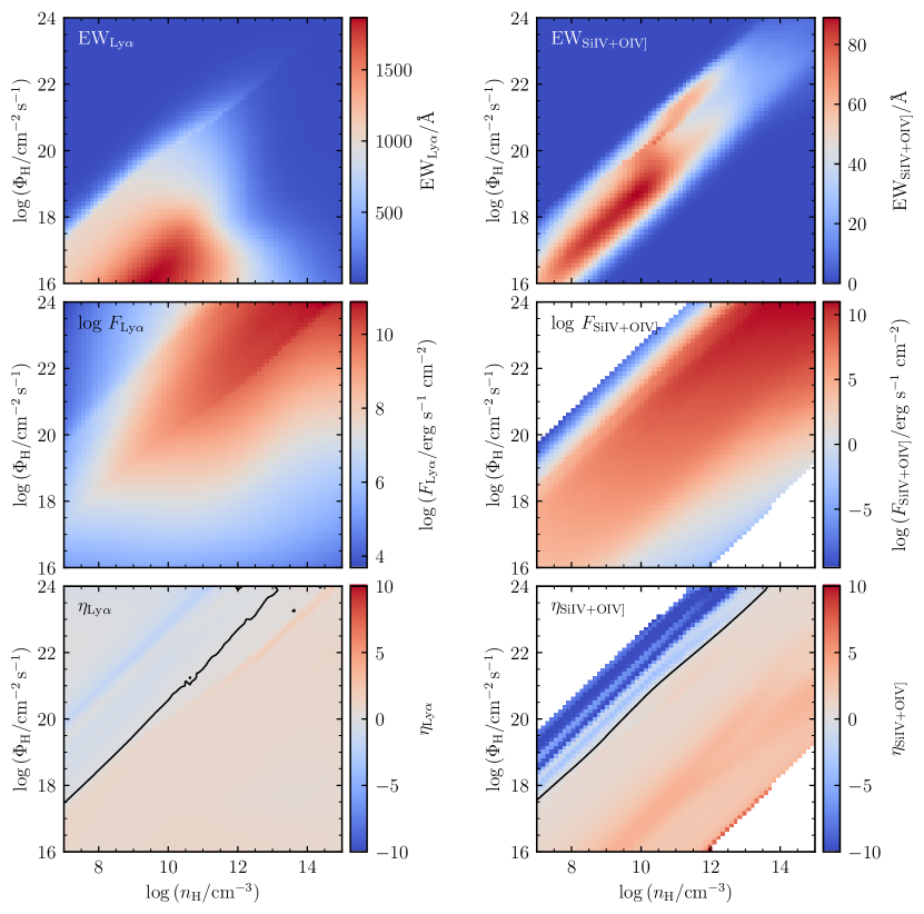
Figure 1: EWs, fluxes, and responsivity of the emission lines for different $n_{\rm H}$ and $\Phi_{\rm H}$. It is obvious that the responsivity tends to be negative if gas density is lower and ionizing continuum is stronger. The solid lines in the lower two panels mark the dividing lines of the positive and negative responsivity.

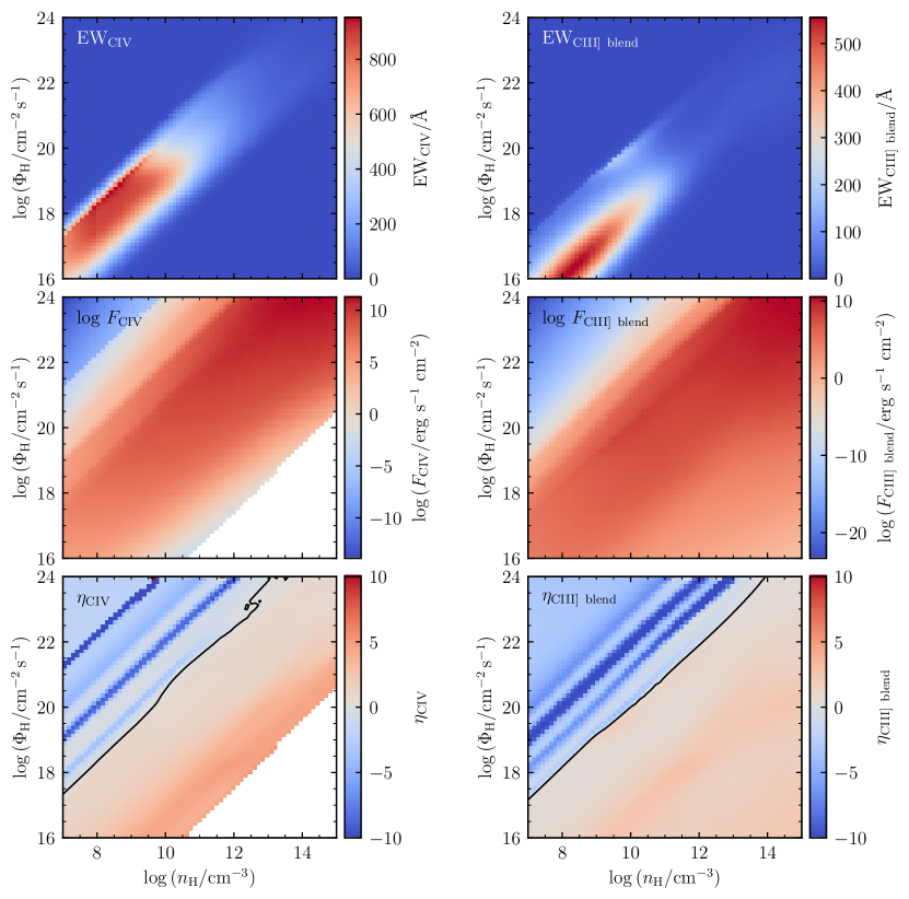
Figure 1: (Continued.)

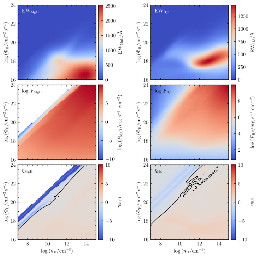
Figure 1: (Continued.)

2 photoionization Calculation

Following the pioneering works of photoionization calculations for the emission-line responses in RM (e.g., Korista & Goad, 2000, 2004), we adopt the locally optimally emitting cloud (LOC, Baldwin et al., 1995) model and perform the calculation using CLOUDY v17.02 (Ferland et al., 2017). We generate a grid of models with gas number density of $7\leqslant\log\ (n_{\rm H}/{\rm cm^{-3}})\leqslant 15$ and surface flux of ionizing photons spanning $16\leqslant\log\ (\Phi_{\rm H}/{\rm cm^{-2}\,s^{-1}})\leqslant 24$. The steps in $n_{\rm H}$ and $\Phi_{\rm H}$ are both 0.125 dex. We assume a simple slab geometry with column density of $10^{23}\ {\rm cm^{-2}}$ (a standard value, see Netzer & Marziani 2010 and references therein) for the line-emitting entities. The typical spectral energy distribution (SED) of Mathews & Ferland (1987) is employed as the ionizing continuum (more discussion is given in Section 5.4). The metallicity is assumed to be solar abundance.

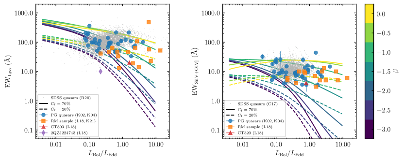
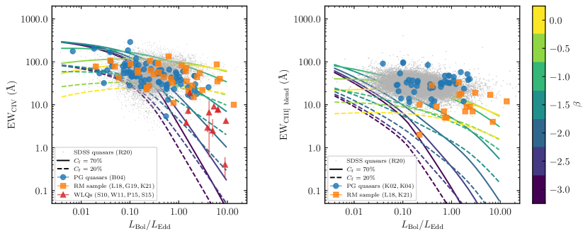
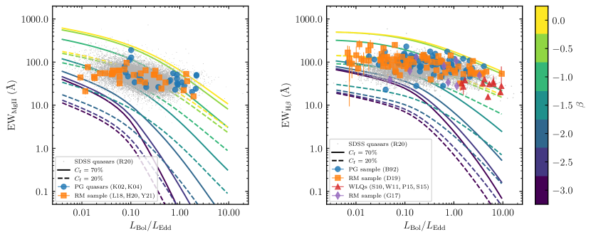
Figure 4: EW vs. Eddington ratio. The lines with different colors are the photoionization models with different $\beta$. The solid and dashed lines are the results for $C_{\rm f}=70\%$ and $20\%$, respectively. The observational points with different symbols in different colors are the samples of RM AGNs, PG quasars, SDSS quasars, and WLQs, which are overlapped for comparison.

We focus on the emission lines that frequently presented in the studies of UV (e.g., Clavel et al., 1991; Grier et al., 2019; Kaspi et al., 2021; Lira et al., 2018; Yu et al., 2021) and optical RM observations (e.g., Peterson et al., 1998; Kaspi et al., 2000; Du et al., 2014; Grier et al., 2017; U et al., 2022). They are Ly$\alpha$ $\lambda 1216$, Si iv$+$O iv] $\lambda 1400$ blend, C iv $\lambda 1549$ doublet, C iii] $\lambda 1909$ blend, Mg ii $\lambda 2798$ doublet, and H$\beta$ $\lambda 4861$ emission lines. There are many other emission lines (Al iii $\lambda\lambda 1855,1863$, Si iii $\lambda\lambda 1883,1892$, and Fe iii $\lambda\lambda 1895,1914,1926$) that are seriously blended with C iii] (see, e.g., Negrete et al., 2012; Temple et al., 2020). They are also added into the flux of C iii] blend.

In order to demonstrate the responses of the BLR clouds to variation of the continuum for different $\Phi_{\rm H}$ and $n_{\rm H}$, we adopt the definition of responsivity ($\eta$) in Korista & Goad (2004). It is defined as

$$\eta=\frac{d\log F_{\ell}}{d\log\Phi_{\rm H}}=\frac{d\log{\rm EW}}{d\log\Phi_{\rm H}}+1.$$ (1)

The responsivities of the BLR clouds with different $n_{\rm H}$ and $\Phi_{\rm H}$ obtained from the photoionization grid, as well as the corresponding EWs and fluxes, are shown in Figure 1. In each panel of the responsivity in Figure 1, a solid line is added as the division of positive and negative values. It is obvious that the responsivity is negative if the gas density is low and the surface flux of the ionizing photons is high (in the upper-left corners of the corresponding panels in Figure 1). This motivates us to consider that the emission-line responses may gradually become negative if the weights of low-density clouds in BLRs increase.

Integrating the line emission over the grid, we can obtain the luminosities of the emission lines. Following Baldwin et al. (1995) and Bottorff et al. (2002), the emission-line luminosity can be obtained by

$$L_{\ell}\propto\int_{n_{\rm min}}^{n_{\rm max}}\!\!\int_{r_{\rm in}}^{r_{\rm out}}r^{2}F_{\ell}(n,r)f(r)g(n)dndr,$$ (2)

where $F_{\ell}(n,r)$ is the line flux of the clouds with gas density $n$ at radius $r$, $f(r)$ is the covering fraction, and $g(n)$ is the gas density distribution. If the ionizing luminosity $L_{\rm ion}$ is given, the radius and the flux of ionizing photons are connected through $\Phi_{\rm H}\propto L_{\rm ion}/4\pi r^{2}$. We assume that both of $f(r)$ and $g(n)$ are simply power laws, namely $f(r)\propto r^{\Gamma}$ and $g(n)\propto n^{\beta}$, where $\Gamma$ and $\beta$ are two indexes. The goal of the present paper is to investigate the potential observational characteristics in RM if the BLR densities change. We fix $\Gamma$ as a constant and keep $\beta$ as a free parameter. As an AGN prototype, the optimal $\Gamma$ in NGC 5548 was suggested to be in the range of $-1.4<\Gamma<-1.0$ (Korista & Goad, 2004). For simplicity, we adopt $\Gamma=-1.0$ in this work.

For typical AGNs, $\beta=-1.0$ is an acceptable assumption (Baldwin et al., 1995; Baldwin, 1997; Korista & Goad, 2004; Guo et al., 2020). Smaller $\beta$ means that most of the BLR clouds have lower gas densities (rarefied BLRs), and larger $\beta$ stands for the BLRs with higher densities (dense BLRs). Here we set $\beta$ from $-3.0$ to $0.0$ to check the influences of gas density to the response behaviors of different emission lines in RM observations. For UV emission lines, we adopt $n_{\rm min}=10^{8}\,{\rm cm^{-3}}$ and $n_{\rm max}=10^{12}\,{\rm cm^{-3}}$ because lower density may lead to some unobserved forbidden lines and higher density makes, e.g., C iv thermalized (Korista & Goad, 2000, 2004). However, hydrogen recombination line can emit efficiently even in much higher density (see Figure 1 and Korista et al. 1997). We loose $n_{\rm max}$ to $10^{15}\,{\rm cm^{-3}}$ for the calculation of the H$\beta$ emission line.

To obtain the emission-line luminosity (Eqn 2), the inner and outer radii ($r_{\rm in}$ and $r_{\rm out}$) of BLRs are required. From Figure 1, the most efficiently emitting clouds are located in relatively a narrow range of $\Phi_{\rm H}$. In the present paper, we pay more attention to the influences of different Eddington ratios than those of the BH masses. For a given BH mass $M_{\bullet}$, we adopt $r_{\rm in}=\sqrt{Q_{0.1}/4\pi\Phi_{\rm H}^{\rm max}}$ and $r_{\rm out}=\sqrt{Q_{0.1}/4\pi\Phi_{\rm H}^{\rm min}}$, where $\Phi_{\rm H}^{\rm min}=10^{18}$ cm^-2 s^-1 and $\Phi_{\rm H}^{\rm max}=10^{22}$ cm^-2 s^-1. $Q_{0.1}$ is the total number of ionizing photons if the Eddington ratio $L_{\rm Bol}/L_{\rm Edd}=0.1$, where $L_{\rm Bol}=\kappa L_{5100}$ is the bolometric luminosity, $\kappa$ is the bolometric correction factor, and $L_{\rm Edd}=1.26\times 10^{38}M_{\bullet}\,{\rm erg\,s^{-1}}$ is the Eddington luminosity. We simply adopt $\kappa=10$ here (e.g., Richards et al., 2006), but caution that $\kappa$ may depend on the accretion rate or SMBH mass (e.g., Jin et al., 2012). The $\Phi_{\rm H}^{\rm min}$ and $\Phi_{\rm H}^{\rm max}$ values we adopted here are just corresponding to $r_{\rm in}=0.1r_{\rm BLR}^{\rm typical}$ and $r_{\rm out}=10r_{\rm BLR}^{\rm typical}$, where $r_{\rm BLR}^{\rm typical}$ is the typical BLR size of the AGNs with $L_{\rm Bol}/L_{\rm Edd}=0.1$ calculated from the classical radius-luminosity (R-L) relationship of $\log(r_{\rm BLR}/{\rm lt\!-\!days})=1.53+0.53\log\ell_{44}$ in Bentz et al. (2013), where $\ell_{44}=L_{5100}/10^{44}\ {\rm erg\ s^{-1}}$ is the monochromatic luminosity at 5100Å. $L_{\rm Bol}/L_{\rm Edd}=0.1$ is roughly the central value of Eddington ratios for nearby Seyfert galaxies and high-redshift quasars ($0.01\lesssim L_{\rm Bol}/L_{\rm Edd}\lesssim 1$, e.g., Boroson & Green 1992; Marziani et al. 2003; Shen et al. 2011; Du & Wang 2019; Wu et al. 2015, and see Figure 4), so the corresponding $r_{\rm BLR}^{\rm typical}$ can be regarded as a typical value. It should be noted that $L_{\rm Bol}/L_{\rm Edd}=0.1$ here is only used for determining a relatively reasonable $r_{\rm in}$ and $r_{\rm out}$. For higher (or lower) ionizing luminosity $L_{\rm ion}$ (or Eddington ratio $L_{\rm Bol}/L_{\rm Edd}$), the most efficiently emitting radius of the line region will spontaneously increases (or decreases) in accordance with $r\propto L_{\rm ion}^{1/2}$. This is known as the physical interpretation for the R-L relationship established from the RM campaigns (e.g., Kaspi et al., 2000; Bentz et al., 2013). Such boundary assumption makes the EW calculation scale-free from BH mass. The dynamic range of radius adopted here is generally large enough for the span of Eddington ratio. We have checked that slightly larger or smaller $r_{\rm in}$ and $r_{\rm out}$ do not influence the general results of the present paper.

3 Equivalent Widths

In Figure 4, we show the dependences of EW on $L_{\rm Bol}/L_{\rm Edd}$ for the emission lines obtained from our photoionization model. The cases with overall covering factors of $C_{\rm f}=20\%$ and $70\%$ are demonstrated. In general, smaller $\beta$ (more rarefied BLR) tends to show weaker EWs. But at the low Eddington-ratio ends of Si iv$+$O iv], C iv, and C iii], large $\beta$ (dense BLR) also produces small EWs.

In order to compare our theoretical calculations with observations and to generally determine the ranges of $\beta$ for different emission lines, we collect the emission-line EWs and $L_{\rm Bol}/L_{\rm Edd}$ from the following samples: (1) the objects from recent RM campaigns or compilations (Grier et al., 2017; Lira et al., 2018; Du & Wang, 2019; Homayouni et al., 2020; Yu et al., 2021; Kaspi et al., 2021), (2) the H$\beta$ (Boroson & Green, 1992) and UV (Kuraszkiewicz et al., 2002, 2004) emission lines of PG quasars, (3) the emission lines of the quasar samples (Calderone et al., 2017; Rakshit et al., 2020) from Sloan Digital Sky Survey (SDSS), and (4) the WLQs from Shemmer et al. (2010), Wu et al. (2011), and Plotkin et al. (2015).

For the RM objects, we can easily calculate their Eddington ratios based on the BH masses obtained from the time lags (Grier et al., 2017; Lira et al., 2018; Du & Wang, 2019; Homayouni et al., 2020; Yu et al., 2021; Kaspi et al., 2021). All of the objects in PG sample have H$\beta$ observations. For the PG quasars without RM measurements, the single-epoch BH masses estimated from their H$\beta$ lines can be used. We employ the simple virial relation to determine their BH masses, namely

$$M_{\bullet}=\frac{fV_{\rm H\beta}^{2}r_{\rm H\beta}}{G},$$ (3)

where $V_{\rm H\beta}$ is the FWHM of H$\beta$ line, $G$ is the gravitational constant, and $f$ is the virial factor. We simply adopt $f=1$ in this paper (e.g., Woo et al., 2015). As aforementioned, the recent works (e.g., Du et al., 2015, 2018; Du & Wang, 2019) discovered that BLR radius (measured from H$\beta$) depends on accretion rate and suggested a new scaling relation for $r_{\rm H\beta}$, which includes the relative strength of Fe ii lines as a new parameter. We calculate the BH masses of the PG objects, which have both H$\beta$ and Fe ii measurements, using the new scaling relation of

$$\log(r_{\rm H\beta}/{\rm lt\!-\!days})=1.65+0.45\log\ell_{44}-0.35R_{\rm Fe}$$ (4)

in Du & Wang (2019), where $R_{\rm Fe}$ is the flux ratio between Fe ii and H$\beta$ lines. For the SDSS quasars with low redshifts which have H$\beta$ observations, the single-epoch BH masses based on the new scaling relation are also used. For the SDSS quasars with high redshifts (with only UV lines), their BH masses and Eddington ratios are based on the classic single-epoch BH mass estimators (see Calderone et al., 2017; Rakshit et al., 2020). It should be noted that the Eddington ratios of the SDSS quasars with high redshifts (for the UV lines) may be underestimated to some extent because their BH masses are obtained based on the classic single-epoch BH mass estimators and the shortening effects of the time lags (e.g., Martínez-Aldama et al., 2020; Dalla Bontà et al., 2020) have not been taken into account. For the WLQs, we only select the objects that have both of C iv and H$\beta$ measurements (Shemmer et al., 2010; Wu et al., 2011; Plotkin et al., 2015). An advantage of selecting these WLQs is that, we can obtain relatively good $M_{\bullet}$ estimates for these objects using the new scaling relation (Du & Wang, 2019), considering that the H$\beta$ emission lines in WLQs are not significantly different from those of normal AGNs (see more details in Section 5.3).

In Figure 4, the emission lines show the Baldwin effects (e.g., Baldwin, 1977) but with different slopes and significances. In general, our photoionization models can cover the distributions of the observational points, which validates the settings of the parameters used in our calculations. Comparing the EW distributions of the current RM samples with those of the other samples, it is obvious that there is still room to improve the completeness of the RM samples. For example, the current RM sample of C iv lacks low-EW objects, especially WLQs, and the H$\beta$ RM sample lines also shows a little bias toward high EWs. On the contrary, more RM observations of Ly$\alpha$, Si iv$+$O iv], and C III] emission lines are needed for high-EW AGNs. Moreover, it is obvious that the objects, which showed anomalous RM behaviors in Lira et al. (2018) (CT320, CT803, and 2QZJ224743), are located at the lower EW ends of the corresponding panels in Figure 4. It implies that their anomalous behaviors may probably connect with weak EWs.

Figure 4 can give a general constraints to the parameter $\beta$ in the context of the photoionization calculations in the present paper. For example, we can determine that the $\beta$ parameter of WLQs roughly ranges from $-2.0$ to $-1.0$ for C iv and from $-0.7$ to $0.0$ for H$\beta$ for the case with $C_{\rm f}=20\%$, and from $-2.5$ to $-1.5$ for C iv and from $-1.2$ to $-0.5$ for H$\beta$ for the case with $C_{\rm f}=70\%$, respectively. It is noted that the observational distributions of the C III] blend in Figure 4 depart slightly from the photoionization calculations. One probable reason is the relatively low abundance (solar abundance) we adopted here (e.g., Snedden & Gaskell 1999, also see Panda et al. 2018, 2019; Śniegowska et al. 2021). We mainly focus on the influence of the BLR densities to the RM behaviors. The influence from abundance will be discussed in a future separate paper (see also Section 5.4 and Appendix A).

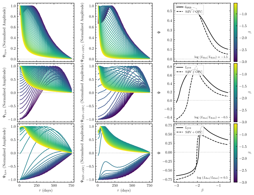
Figure 5: One-dimensional transfer functions $\Psi$ of the emission lines for different $\beta$. The transfer functions are color coded by the $\beta$ parameter. $\bar{\Psi}$ is the average of the transfer function. The cases with $\log(L_{\rm Bol}/L_{\rm Edd})=-1.5$, $-0.5$ and $0.5$ are shown, respectively. The emission lines tend to show negative responses to the varying continuum in RM observations if $\beta$ is smaller.

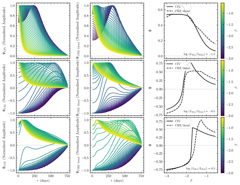
Figure 5: (Continued.)

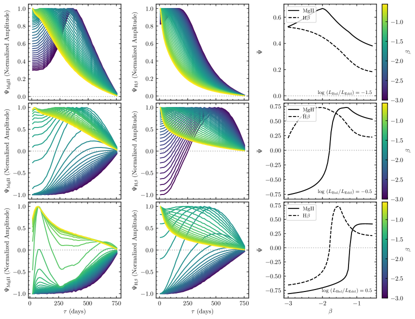
Figure 5: (Continued.)

4 Transfer function

In RM, the delayed response of an emission line to the varying continuum can be characterized by the transfer function (Blandford & McKee, 1982) in the form of

$$\Delta F_{\ell}(t)=\int_{-\infty}^{+\infty}\Delta F_{\rm c}(t^{\prime})\Psi(t-t^{\prime})dt^{\prime},$$ (5)

where $\Delta F_{\rm c}(t)$ and $\Delta F_{\ell}(t)$ are the variations of the continuum and emission-line fluxes, and $\Psi(t)$ is the one-dimensional transfer function. Transfer function $\Psi$ connects the emission-line light curve with the continuum variation (Blandford & McKee, 1982), and can be easily obtained from RM observations by different algorithms and softwares, e.g., the maximum entropy method (e.g., Krolik et al., 1991; Horne et al., 1991), JAVELIN (Zu et al., 2011), MICA (Li et al., 2016), and Pixon (Li et al., 2021). Some examples of the one-dimensional transfer functions reconstructed from RM observations can be found in, e.g., Grier et al. (2013), Williams et al. (2018), and Bao et al. (2022). From the photoionization grid in Section 2, we can calculate the one-dimensional transfer functions by

$$\Psi(\tau)\propto\int_{r_{\rm in}}^{r_{\rm out}}\int_{0}^{\pi}\int_{0}^{2\pi}\eta(r)f(r)F_{\ell}(r)r^{2}\sin\theta\\ \times\delta\left[\tau-\frac{r+\vec{r}\cdot\vec{n}_{\rm obs}}{c}\right]drd\theta d\phi,$$ (6)

where

$$F_{\ell}(r)=\int_{n_{\rm min}}^{n_{\rm max}}F_{\ell}(n,r)g(n)dn,$$ (7)

is the emission-line flux at radius $r$ obtained by integrating $F(n,r)$ over density $n$,

$$\eta(r)=-0.5\frac{d\log F_{\ell}(r)}{d\log r}$$ (8)

is the responsivity function at radius $r$ derived from Eqn (1), $\tau$ is the time, $\vec{n}_{\rm obs}$ is the line of sight, $c$ is the speed of light, and ($\theta$, $\phi$) are the angles of the spherical coordinates. The purpose of this paper is to investigate the influence of BLR densities to the transfer functions. Therefore, for simplicity, we assume that the BLR geometry is spherically symmetric.

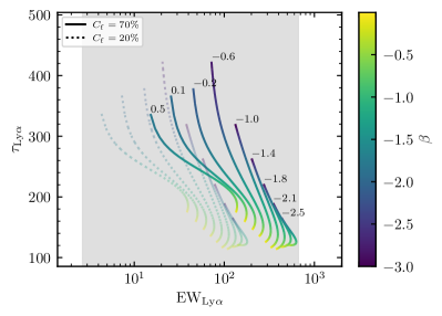
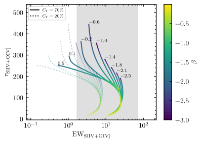
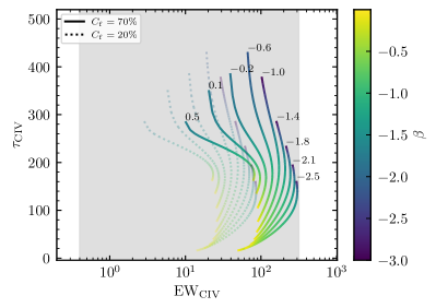
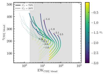
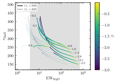
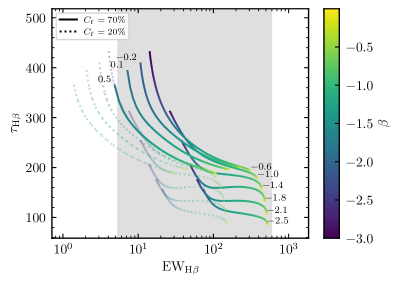
Figure 8: The correlations between EWs and time lags. The solid and dashed lines are the cases of $C_{\rm f}=70\%$ and $C_{\rm f}=20\%$, respectively. Each line has the same luminosity or Eddington ratio, and is color-coded by $\beta$. The Eddington ratio is marked nearby the corresponding line. The observations of the EW ranges of different emission lines (in Figure 4) are also overlapped in grey.

We calculate the transfer functions for different $\beta$ and show the results in Figure 5 for three cases of different Eddington ratios [$\log(L_{\rm Bol}/L_{\rm Edd})=-1.5$, $-0.5$, and $0.5$]. The mass of SMBH is set to be $10^{8}M_{\odot}$. Generally speaking, at low Eddington ratios, the transfer functions are always positive and their peaks (with the strongest responses) move toward longer time lags if $\beta$ decreases (more rarefied BLRs). Along with Eddington ratio increases, the transfer functions with smaller $\beta$ (more rarefied BLRs) still have longer time lags than those with larger $\beta$ (denser ones), however their amplitudes become from positive to negative. Negative transfer functions mean that the emission-line light curves show inverse responses with respect to the variations of the continuum light curves, which are different from the usual cases in RM. To quantify whether or not the response is negative in average, we calculate the average of a transfer function by $\bar{\Psi}=\int\Psi(t)dt/\int dt$. $\bar{\Psi}$ for different $\beta$ are also shown in Figure 5. The transition from positive $\bar{\Psi}$ to negative $\bar{\Psi}$ happens at larger $\beta$ if Eddington ratio increases. More specifically, different lines show different behaviors. At the same Eddington ratio, it is easier for the responses of Mg ii, C iv, and C iii] to become negative than those of Ly$\alpha$, Si iv$+$O iv], and H$\beta$. The transitions of Mg ii, C iv, and C iii] occur at relatively larger $\beta$. For example, Mg ii can become negative at $\log(L_{\rm Bol}/L_{\rm Edd})=-0.5$, however the average responses of H$\beta$ keep positive in the same case.

The $\beta$ parameter controls both of EWs and typical BLR radii (time lags), therefore we can investigate their correlations. We define an average time lag of a transfer function using the formula of

$$\tau=\int t\Psi(t)dt/\int\Psi(t)dt.$$ (9)

Through adjusting $\beta$, we can show the correlations between time lags and EWs in Figure 8. It should be noted that this definition is not appropriate if $\Psi(t)$ is partly negative. Considering that currently only positive transfer functions are thought to be “successful” in RM observations, we plot the cases of purely positive transfer functions here. Therefore, the curves for high Eddington ratios in Figure 8 are cut off at small $\beta$ (see, e.g., the cases of C iv for $\log(L_{\rm Bol}/L_{\rm Edd})=0.1$ and $0.5$ in Figure 8).

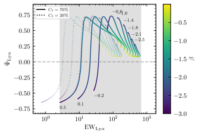
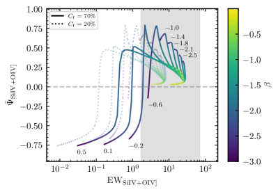
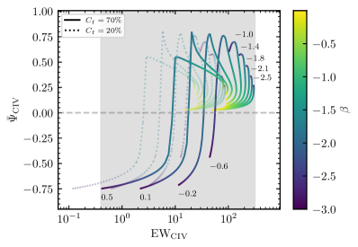
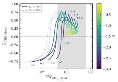
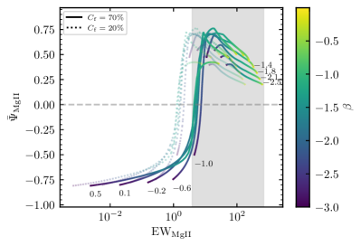
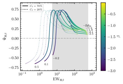
Figure 9: The correlations between EWs and the amplitudes of transfer functions. The solid and dashed lines are the cases of $C_{\rm f}=70\%$ and $C_{\rm f}=20\%$, respectively. Each line has the same luminosity or Eddington ratio, and is color-coded by $\beta$. The Eddington ratio is marked nearby the corresponding line. The observations of the EW ranges of different emission lines (in Figure 4) are also overlapped in grey.

In Figure 8, each line has the same luminosity or Eddington ratio, and is color-coded by the parameter $\beta$. These correlations mean that the diverse density distributions of BLRs can result in variations of EWs (by nearly an order of magnitude) and time lags (by factors of $\sim$2-3) simultaneously even if the luminosities are the same. This may contribute to the scatters ($\sim$0.3dex) of the $R$-$L$ relationships of the emission lines and may also be one of the explanations for the variations of time lags in individual objects in different years. However, the correlations between time lags and EWs are different in different emission lines. Ly$\alpha$, Si iv$+$O iv], C iv, and C iii] show nonmonotonic correlations. In these four emission lines, along with $\beta$ increasing, the time lags continuously become shorter, however the EWs first increase and then decrease after across their maximums. For the other two lines (Mg ii and H$\beta$), both of the time lags and EWs show almost monotonic correlations with $\beta$. $\beta$ shows correlations (and anti-correlations) with their EWs (and time lags). More specifically, for the three primary emission lines in RM - C iv, Mg ii, and H$\beta$, they have the following typical characteristics.

C iv: The EWs and time lags mainly show positive correlations at low Eddington ratios [e.g., $\log(L_{\rm Bol}/L_{\rm Edd})=-2.5$ and $-2.1$] and anti-correlations at high Eddington ratios [e.g., $\log(L_{\rm Bol}/L_{\rm Edd})=0.1$ and $0.5$]. The change of BLR density ($\beta$) causes the variation of time lag but only weakly influence the EWs at moderate Eddington ratios [e.g., $\log(L_{\rm Bol}/L_{\rm Edd})=-0.6$].

Mg ii: The EWs and time lags are mainly anti-correlated. Time lag decreases if EW increases at almost all Eddington ratios. However, the slopes are steeper at low EWs than those at high EWs.

H$\beta$: The behavior of H$\beta$ line is more similar to that of Mg ii line. However, at high EWs (e.g., ${\rm EW}\gtrsim 80$-$100$ for the cases of $C_{\rm f}=70\%$ and ${\rm EW}\gtrsim 30$-$40$ for the cases of $C_{\rm f}=20\%$), the variations of the time lags are very weak along with the change of $\beta$.

Here we do not plot the RM observations in Figure 8 because the exact values of time lags are also significantly controlled by BLR geometry, which is simply assumed to be spherically symmetric in our calculations (may be very different from the actual situations). But we can generally do a simple comparison. Du & Wang (2019) shows the correlation between $\Delta R_{\rm H\beta}=\log\,(R_{\rm H\beta}/R_{\rm H\beta,R-L})$ and ${\rm EW_{H\beta}}$, where $R_{\rm H\beta,R-L}$ is the H$\beta$ lag calculated from the $R$-$L$ relationship. Each line in Figure 8 has the same luminosity. Therefore, we can compare the observed $\Delta R_{\rm H\beta}$-${\rm EW_{H\beta}}$ correlation with our calculations. In Du & Wang (2019), except for those super-Eddington AGNs, the AGNs with normal accretion rates (with $70<{\rm EW_{H\beta}}<300$) do not show any significant $\Delta R_{\rm H\beta}$-${\rm EW_{H\beta}}$ correlation or anti-correlation. This is generally consistent with our calculations that ${\rm EW_{H\beta}}$ and $\tau_{\rm H\beta}$ do not show strong correlation at relatively high EWs. From our calculations, we expect that more high-quality observations of the H$\beta$ with weaker EWs in AGNs with normal accretion rates in future may discover some objects with longer time lags than the $R$-$L$ relationship.

In addition, we simply check the RM samples of C iv lines (Lira et al., 2018; Grier et al., 2019; Kaspi et al., 2021) and obtain a very weakly positive $\Delta R_{\rm CIV}$-${\rm EW_{CIV}}$ correlation with Spearman’s rank correlation coefficient of $\rho=0.32$ and a corresponding $p$-value of $0.09$ based on the C iv $R$-$L$ relationship in Kaspi et al. (2021). Considering that the $\beta$ values of the current C iv RM samples are relatively large (see Figure 4), this may probably be consistent with our calculations, especially the parts with $\tau<200$ days in Figure 8. Similarly, we also perform a test to the Mg ii samples (Lira et al., 2018; Homayouni et al., 2020; Yu et al., 2021) based on the $R$-$L$ relationship in Homayouni et al. (2020). However, no significant correlation is found ($\rho=0.09$ and $p=0.61$). One possible reason is the relatively narrow EW span (0.16dex) of the current Mg ii RM samples (Lira et al., 2018; Homayouni et al., 2020; Yu et al., 2021). As a comparison, the EW span of C iv RM samples (Lira et al., 2018; Grier et al., 2019; Kaspi et al., 2021) is 0.30dex.

Through adjusting $\beta$, we can also plot the correlation between $\bar{\Psi}$ and EW in Figure 9 in order to check the EW at which the transition from averagely positive to negative response happens. From Figure 9, C iv, Ly$\alpha$ are more easier to show negative (anomalous) responses in RM because the grey ranges cover more cases with negative $\bar{\Psi}$. The observations of the other four lines can also cover the negative responses from the photoionization calculations, however only if the EWs are very close to the lower limits.

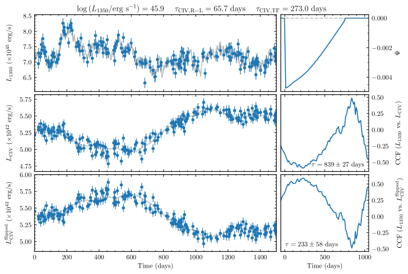
Figure 10: An example of C iv light curve if $\beta=-2.0$. The grey lines are the mock light curves, and the blue points are the mock data by adding some artificial uncertainties ($10\%$) with a sampling cadence of 10 days. The upper-left panel ($L_{1350}$) is the continuum light curve (from simple DRW model) in 1350Å. The middle-left panel ($L_{\rm CIV}$) is the C iv light curve. The lower-left panel ($L_{\rm CIV}^{\rm flipped}$) is the flipped C iv light curve. The upper-right panel shows the transfer function $\Psi$. The middle-right panel is the CCF obtained from $L_{1350}$ vs. $L_{\rm CIV}$, which is the conventional analysis in RM but gives a wrong time lag ($\tau=839\pm 27$ days) with respect to the input value ($\tau_{\rm CF,TF}=273.0$ days). The CCF from $L_{1350}$ vs. $L_{\rm CIV}^{\rm flipped}$ is provided in the lower-right panel and can yield the correct time lag ($\tau=233\pm 58$ days). The input luminosity and the time lag from the transfer function are shown on the top. $\Psi$ is in arbitrary unit.

5 Discussion

5.1 Implication for RM observations

As mentioned in Section 1, there are already several objects showing anomalous behaviors in RM observations (especially CT 320, CT 803, and 2QZ J224743 in Lira et al. 2018). The Si iv line of CT 320 and the Ly$\alpha$ line of CT 803 and 2QZ J224743 show obviously negative responses (see their light curves in Figure 5 of Lira et al. 2018). Their emission-line light curves are inversely correlated with the continuum variations. The corresponding cross correlations (CCFs) in Lira et al. (2018) exhibit strong troughs with minimum cross-correlation coefficients smaller than $-0.5$. Positive peaks with such amplitudes ($0.5$) in CCFs commonly represent significant responses. These anomalous RM responses may probably be explained by their low BLR densities.

In consideration of the possible negative responses of emission lines in rarefied BLRs, it will lead to some troubles if their RM data are analyzed according to traditional experiences. We demonstrate an example of the C iv negative response in Figure 10. It is obvious that the emission-line light curve inversely responses the continuum light curve. In this case, we adopt $\beta=-2.0$ and $\log(L_{\rm Bol}/L_{\rm Edd})=0.5$. For simplicity, the continuum light curve is assumed to be a damped random walk (e.g., Zu et al., 2013), which applies to most of AGNs (e.g., Kasliwal et al., 2015). The monochromatic luminosity is $\log(L_{1350}/{\rm erg\ s^{-1}})=45.9$, and the corresponding time lag is $\tau_{\rm CIV,R-L}=65.7$ days based on the C iv R-L relationship in Kaspi et al. (2021). The transfer function $\Psi$ is totally negative in this case. The mean time lag calculated from transfer function is $\tau_{\rm CIV,TF}=273.0$ days (Eqn 9). To simulate observed light curves, some artificial error bars (10% for both continuum and emission line) are added.

Conventionally, RM measures the time lag between the continuum and emission-line light curves using CCF in order to determine the mass of SMBH. However, in this simple example, we obtain a very different time lag of $\tau=839\pm 27$ days (directly from the strongest positive peak in the CCF) comparing with the above input value ($\tau_{\rm CIV,TF}$) if we perform the time-series analysis directly to the mock light curves using interpolated CCF (Gaskell & Peterson, 1987). The error bar of the time lag is obtained by the “flux randomization/random subset sampling” method (e.g., Peterson et al., 1998, 2004). This time lag is obviously incorrect. The low peak correlation coefficient ($<0.5$) also indicates that the continuum and emission-line light curves are poorly correlated.

If we flip the emission-line light curve, we can get a reliable time lag of $\tau=233\pm 58$ days, which is consistent with the input $\tau_{\rm CIV,TF}$ within $1\sigma$ uncertainties. The peak correlation coefficient between the continuum and the flipped emission-line light curves is much higher (close to 0.7). Therefore, we need to flip the emission-line light curves in the time-series analysis for such rarefied BLRs if we hope to get reliable time lags.

In practice, the maximum and minimum correlation coefficients in CCF can be used as a criterion to identify the rarefied BLRs in real data. If the absolute value of the minimum correlation coefficient is significantly larger than that of the maximum correlation coefficient in an object with very small emission-line EW and high Eddington ratio, it is probably a source with rarefied BLR and should be analyzed by flipping its emission-line light curve.

5.2 Justify Anemic BLR Model from RM Observations

The physics behind WLQs has not been fully understood yet. Several models were proposed to explain the origin of their emission-line weakness, and can generally be divided into two categories. The first category is based on unusual ionizing continuum (the deficit of ionizing photons from accretion disks) due to, e.g., high accretion rates (Leighly et al., 2007a, b), the absorption by some shielding gas (Wu et al., 2011), the shielding by the puffed-up inner region of the slim accretion disks (Luo et al., 2015), or even the very cold accretion disks in hyper-massive black holes (Laor & Davis, 2011). The second category is the anemic BLR model in which the BLRs themselves are lack of gas (e.g., Shemmer et al., 2010). The BLRs are probably in the very early stage of formation (Hryniewicz et al., 2010; Wang et al., 2012; Andika et al., 2020). A question which arises is how can we further reveal what happens in WLQs?

From the above photoionization calculations, we predict that the anemic BLR may lead to negative response of C iv lines with respect to the continuum variation in RM observations. We propose that RM can be used to verify the anemic BLR model in WLQs. From Figure 4, we can obtain a general constraints to the $\beta$ parameters in WLQs. The $\beta$ parameters of C iv and H$\beta$ emission lines in WLQs have been constrained to be within the ranges of [$-2.0$, $-1.0$] and [$-0.7$, $0.0$] for the case with $C_{\rm f}=20\%$, and [$-2.5$, $-1.5$] and [$-1.2$, $-0.5$] for the case with $C_{\rm f}=70\%$, respectively. The response behaviors of these two lines are different. The C iv lines in WLQs can have negative $\bar{\Psi}$ (especially for those with $-2.5<\beta<-1.75$). However, from the photoionization calculations and the range of $\beta$, the H$\beta$ emission lines in WLQs do not have similar behaviors. The H$\beta$ lines of WLQs (at least the current WLQ samples) only positively response to the variations of the continuum radiation.

Therefore, from the negative response of C iv emission line to the variation of the continuum, it is possible to validate the anemic BLR model of the WLQs. If some WLQs are found to show negative C iv response in RM observations, it implicates that the anemic BLR model works (at least in some WLQs). On the contrary, if none of the C iv in WLQs exhibits any negative response, the anemic model doesn’t work and the model based on unusual ionizing continuum may play a key role in WLQs.

Because of the weakness of the emission lines in WLQs, high-fidelity RM observations with highly-accurate flux calibration from large-aperture telescopes are required (e.g., Gemini 8.1 m, Magellan 6.5 m telescopes). Considering that the typical EWs of C iv in WLQs are lower than their normal counterparts by roughly factors of 5$\sim$10, the accuracy of flux calibration should be as good as $0.5\%\sim 1\%$ (given that the typical error bars of the current C iv RM observations are $4\sim 5\%$, see, e.g., Lira et al. 2018; Kaspi et al. 2021). There is no any narrow emission lines in the UV spectra of WLQs in their rest frames, the traditional narrow-line-based calibration method in RM (e.g., Peterson et al., 1998; Bentz et al., 2009; Grier et al., 2017) cannot be performed in WLQs. Instead, the comparison-star-based calibration (Kaspi et al., 2000, 2021; Du et al., 2014) should be adopted. This method can in principle provide good calibration accuracy ($\sim 1\%$) in relatively good weather condition.

Using the latest R-L relation (e.g., Lira et al., 2018; Hoormann et al., 2019; Grier et al., 2019; Kaspi et al., 2021), the time lags of C iv can be estimated if the monochromatic luminosities are given. However, the phenomenon of shortened time lags in high accretion rate AGNs found in H$\beta$ emission lines (e.g., Du et al., 2015, 2016, 2018) may also play roles in C iv lines (Dalla Bontà et al., 2020). WLQs have relatively high accretion rates (Leighly et al., 2007a, b; Luo et al., 2015, see also Figure 4). Therefore, the sampling cadences for WLQs need to be higher than the expected from the C iv R-L relation.

It should be noted that the shielding gas model of WLQs may also lead to anomaly in the emission-line responses, similar to the cases of “BLR holiday” in NGC 5548 (Goad et al., 2016; Pei et al., 2017) and Mrk 817 (Kara et al., 2021) that the continuum and emission-line light curves are decoupled. The changes of the properties (density, covering factor, etc.) of the shielding gas (or disk wind, Wu et al., 2011; Luo et al., 2015; Jin et al., 2022) can mainly influence the emission line but do not significantly affect the continuum if the shielding gas is not in the line of sight. In this case, the continuum and emission-line light curves may probably show weak (or even no) correlations. This kind of anomaly is different from the negative responses discussed in the present paper.

5.3 Possible Explanation for Weak C iv and Normal H$\beta$: Radiation Pressure

A puzzle in WLQs is why high ionization lines (e.g., C iv) show relatively weak EWs however low ionization lines (like H$\beta$) do not. One possibility is that the ionizing continuum for the BLRs in WLQs is unusually soft due to super-Eddington accretion (Leighly et al., 2007a, b), shielding gas (Wu et al., 2011), the central puffed-up inner regions of slim disks (Luo et al., 2015), or the code accretion disks in hyper-massive AGNs (Laor & Davis, 2011). The other possibility is that the gas clouds of high- and low-ionization lines have different physical properties in “anemic” model (Plotkin et al., 2015). In the context of our photoionization calculation, the observations of C iv and H$\beta$ EWs indicate that only C iv emitting clouds suffer “anemia” however the H$\beta$ clouds tend to be more “normal”. Only $\beta_{\rm CIV}$ becomes significantly smaller than $-1$ in WLQs, but $\beta_{\rm H\beta}$ is still close to $-1$ (see Figure 4 and Section 5.2).

It has been known for many years that the C iv lines in AGNs tend to show blueshifted profiles which are usually interpreted by outflow kinematics (e.g., Marziani et al., 1996; Baskin & Laor, 2005; Richards et al., 2011). A clear demonstration of the C iv outflow came from the RM observation of NGC 5548 in UV band (Bottorff et al., 1997). On the contrary, the outflow kinematics is relatively rare in the H$\beta$ emitting region. The velocity-resolved RM reveals that the H$\beta$ kinematics of most AGNs are dominated by virialized motion or inflow (e.g., Bentz et al., 2010; Grier et al., 2013; De Rosa et al., 2018; Bao et al., 2022, or see Figure 14 in U et al. 2022). The high-quality two-dimensional transfer function of H$\beta$ in NGC 5548 shows that its H$\beta$ region is a Keplerian rotating disk (Xiao et al., 2018; Horne et al., 2021).

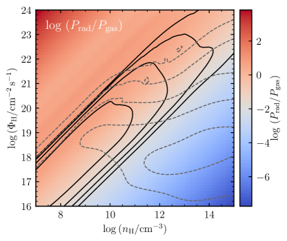
Figure 11: Ratio between radiation pressure ($P_{\rm rad}$) and gas pressure ($P_{\rm gas}$). The EW contours of C iv (solid lines) and H$\beta$ (dashed lines) are overlayed. It is obvious that the radiation pressure on the C iv-emitting clouds are much stronger than the H$\beta$-emitting clouds.

We check the radiation pressure $P_{\rm rad}$ (due to the attenuation of the incident continuum) and gas pressure $P_{\rm gas}$ of the photoionization grid in Section 2. The ratio $P_{\rm rad}/P_{\rm gas}$ overlayed with the contours of the C iv and H$\beta$ EWs is shown in Figure 11. It is obvious that the radiation pressure acting on the clouds is generally larger than the gas pressure in the C iv emitting region, but smaller in the H$\beta$ region. This may probably explain, at least in the framework of anemic BLR model, why only C iv lines become much weaker in WLQs. The large radiation pressure on C iv clouds may drive strong outflow and push the medium away. This process undoubtedly reduces the gas content (gas density). WLQs have generally higher Eddington ratios than normal quasars and hence stronger radiation pressures (stronger C iv outflow). The radiation pressure on H$\beta$ clouds is much weaker, therefore the gas is still bounded by the gravitational potential of the central SMBH. This speculation is also consistent with the vertical geometry of BLRs in Kollatschny & Zetzl (2013) that C iv clouds are relatively far away from the mid-plane (blown away by radiation pressure) but H$\beta$ is emitted in a more flattened geometry.

The other UV lines aforementioned also have similar behaviors as C iv. Si iv$+$O iv] and C iii] emitting clouds may suffer stronger radiation pressure. The radiation pressure may be slightly weaker on Ly$\alpha$ clouds, and much weaker on Mg ii clouds. Therefore, the WLQ phenomena and anomalous responses on Si iv$+$O iv], C iii], and Ly$\alpha$ may probably stronger than Mg ii.

5.4 Other Factors: SED, metallicity, $\Gamma$, and Covering Factor?

We adopted the SED from Mathews & Ferland (1987) in our photoionization calculation. However, SED depends on BH masses and Eddington ratios of AGNs (e.g., Jin et al., 2012; Ferland et al., 2020, and references therein). In addition, the BLR metallicity is probably higher in the AGNs with high accretion rates (e.g., Panda et al., 2019; Śniegowska et al., 2021). Considering that WLQs have high accretion rates (e.g., Shemmer et al., 2010; Wu et al., 2011; Plotkin et al., 2015, see also Figure 4), we adopt a different input configuration (with the SED for the highest Eddington ratio in Ferland et al. (2020) and higher metallicity) and run the calculation again as a test (see more details in Appendix A). A smaller $\Gamma$ is also adopted here. We find that the general conclusions in the present paper (e.g., EW vs. $\bar{\Psi}$ and negative response of C iv) do not change significantly (see Appendix A). More realistic calculations are still needed in future.

Actually, the other possibility of the anemic BLR model is that WLQs have very anomalous covering factor of their BLR clouds but similar gas densities as their normal counterparts. If this is the case, their C iv will not show negative responses to the varying continuum.

Note that here we assume the BLR geometry is spherically symmetric, which could be too simple. The true BLRs may be thick disks or even more complex geometry or kinematics (inflow or outflow, e.g., see Pancoast et al. 2014; Williams et al. 2018; Villafaña et al. 2022). Comparing with the spherically symmetric cases in the present paper, the major difference of thick BLR disks is that they have fewer gas clouds and/or lower gas density at the regions in the polar directions and relatively far away from the central ionizing sources. Therefore, it is expected that the transfer functions in thick BLR disks will be narrower than the cases shown in the present paper, and/or the responses may become negative at relatively larger $\beta$. However, the general tendency, that rarefied BLRs (small $\beta$) show negative responses, will remain the same. We will perform more sophisticated calculation for practical BLR geometry and kinematics in future.

6 Summary

In this paper, we present photoionization calculations (LOC models) for the one-dimensional transfer functions of Ly$\alpha$ $\lambda 1216$, Si iv$+$O iv] $\lambda 1400$ blend, C iv $\lambda 1549$ doublet, C iii] $\lambda 1909$ blend, Mg ii $\lambda 2798$ doublet, and H$\beta$ $\lambda 4861$ emission lines in order to investigate the roles of BLR densities in their RM observations. Based on the calculations and the comparison with observations, we have the following predictions and conclusions:

• The AGNs with rarefied BLRs (small $\beta$) are predicted to show negative responses (anomalous responses) in RM observations. The emission lines of such objects may have relatively low EWs. The observed anomalous behaviors in the UV emission lines of some objects in the past RM campaigns (e.g., CT 320, CT 803, and 2QZ J224743 in Lira et al. 2018) may be explained by the rarefied BLRs. In this case, the emission-line light curves may need to be flipped before the time-series analysis if we want to get accurate BLR radii.

• The different BLR densities in AGNs may contribute to the scatter of the $R$-$L$ relationship. The wide distributions of the BLR densities can result in changes of time lags by factors of 2-3. Preliminarily, the observed scatter of the C iv $R$-$L$ relationship is probably consistent with the calculations in the present paper. For the other emission lines (Mg ii and H$\beta$), more RM observations for the AGNs with wider EW spans are needed.

• The variation of time lags in individual objects without significant changes of continuum luminosities may be explained by the changes of BLR densities with time.

• We propose that the existence of negative responses in C iv RM observations can be used to justify if the anemic BLR model works or not in WLQs. If negative responses are found in WLQs, their emission-line weakness can be attributed to the deficit of BLR gas.

Appendix A A Test for Input Configuration

The input configuration (SED, BLR metallicity, and $\Gamma$) adopted in our photoionization calculation of the main text is appropriate for typical quasars. However, WLQs tend to have higher accretion rates (e.g., Shemmer et al., 2010; Wu et al., 2011; Plotkin et al., 2015, see also Figure 4), thus this configuration may be not ideal for WLQs. Here we change the configuration and run the calculation again for comparison. We adopt the SED for the highest Eddington ratio in Ferland et al. (2020) and a metallicity of $5Z_{\odot}$, where $Z_{\odot}$ is the solar abundance (the metallicity of high-accretion-rate quasars are higher, see, e.g., Panda et al. 2019; Śniegowska et al. 2021). The BLR sizes of the AGNs with high accretion rates measured from RM are smaller than the predictions of the $R$-$L$ relation (e.g., Du et al., 2015, 2018), which may possibly imply that their BLR clouds are more concentrated in the central regions (corresponding to smaller $\Gamma$). We thus adopt $\Gamma=-1.5$. The other parameters are kept the same as the main text. We call this configuration “Configuration B” (The input for the photoionization calculation in the main text is called “Configuration A”). The results of Configuration B are shown in Figures 12-20.

We find the general results do not change significantly. For example, if $\beta$ decreases, the transfer function tend to become negative, especially for the cases with high Eddington ratios. The correlations between EWs and time lags may contribute to the scatters of the $R$-$L$ relations. These are almost the same as the results of Configuration A. But there are still some small differences that we noticed. (1) The responsivities of Ly$\alpha$ and H$\beta$ in Figure 12 have small positive zones in the high $\Phi_{\rm H}$ and low $n_{\rm H}$ regions. (2) With the same Eddington ratio, the transfer functions of Configuration B can become negative at larger $\beta$ (see Figure 5 and 16). (3) The correlations between EWs and time lags for Si iv$+$O iv, C iv, and C iii blend are more monotonic (see Figure 19), which are a little different from the nonmonotonic correlations in Figure 8.

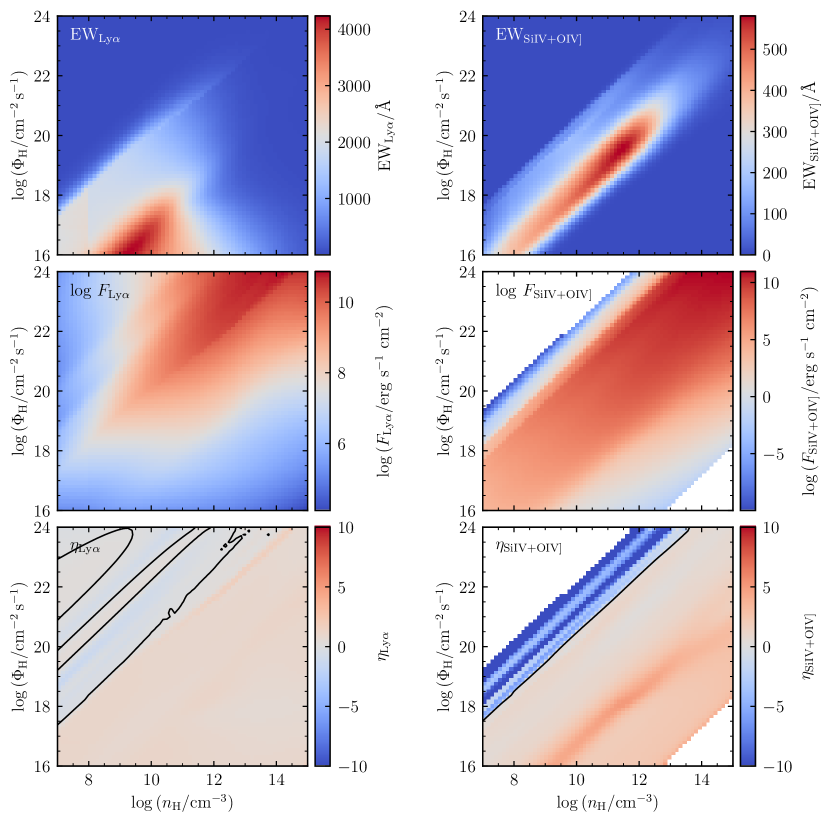
Figure 12: EWs, fluxes, and responsivity of the emission lines for different $n_{\rm H}$ and $\Phi_{\rm H}$ (Configuration B). The meanings of the panels, colors, and lines are the same as Figure 1.

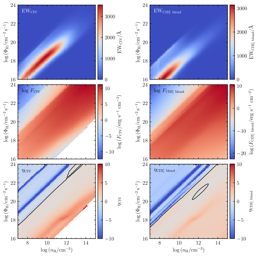
Figure 12: (Continued.)

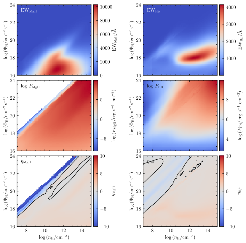
Figure 12: (Continued.)

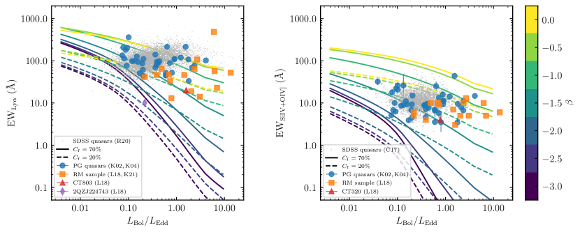
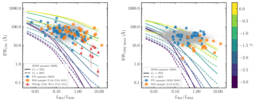
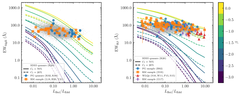
Figure 15: EW vs. Eddington ratio (Configuration B). The meanings of the panels, colors, lines, and symbols are the same as Figure 4.

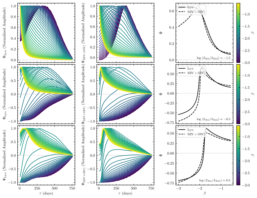
Figure 16: One-dimensional transfer functions $\Psi$ of the emission lines for different $\beta$ (Configuration B). The meanings of the panels, colors, and lines are the same as Figure 5.

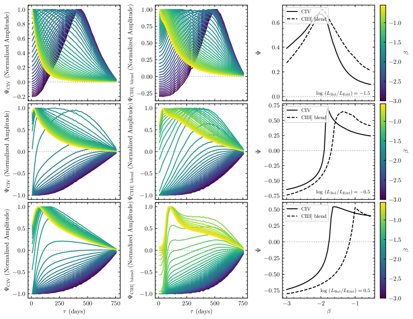
Figure 16: (Continued.)

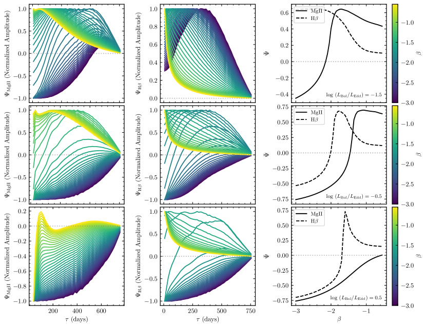
Figure 16: (Continued.)

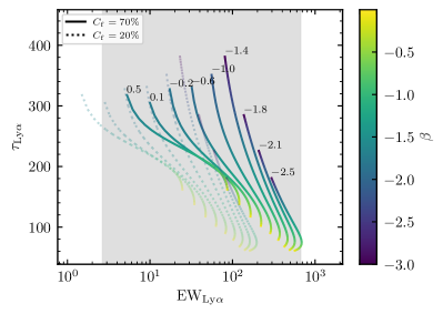
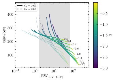
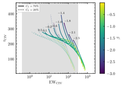
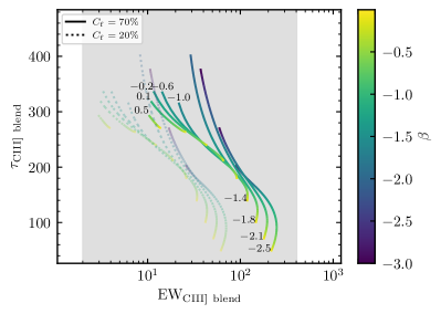
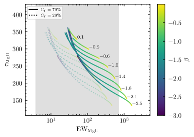
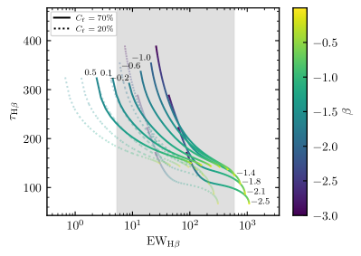
Figure 19: The correlations between EWs and time lags (Configuration B). The meanings of the panels, colors, and lines are the same as Figure 8.

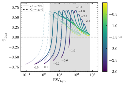
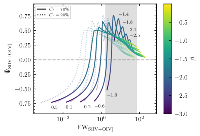
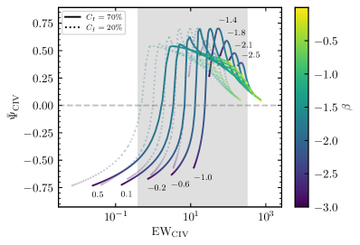
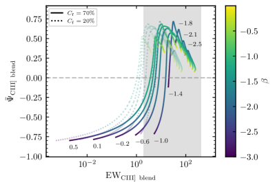
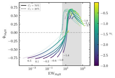
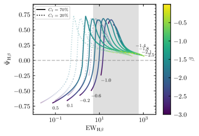
Figure 20: The correlations between EWs and the amplitudes of transfer functions (Configuration B). The meanings of the panels, colors, and lines are the same as Figure 9.

References

- Anderson et al. (2001) Anderson, S. F., Fan, X., Richards, G. T., et al. 2001, AJ, 122, 503. doi:10.1086/321168
- Andika et al. (2020) Andika, I. T., Jahnke, K., Onoue, M., et al. 2020, ApJ, 903, 34. doi:10.3847/1538-4357/abb9a6
- Bahcall et al. (1972) Bahcall, J. N., Kozlovsky, B.-Z., & Salpeter, E. E. 1972, ApJ, 171, 467. doi:10.1086/151300
- Baldwin (1977) Baldwin, J. A. 1977, ApJ, 214, 679. doi:10.1086/155294
- Baldwin et al. (1995) Baldwin, J., Ferland, G., Korista, K., et al. 1995, ApJ, 455, L119. doi:10.1086/309827
- Bao et al. (2022) Bao, D.-W., Brotherton, M. S., Du, P., et al. 2022, arXiv:2207.00297
- Baldwin (1997) Baldwin, J. A. 1997, IAU Colloq. 159: Emission Lines in Active Galaxies: New Methods and Techniques, 113, 80
- Baskin & Laor (2005) Baskin, A. & Laor, A. 2005, MNRAS, 356, 1029. doi:10.1111/j.1365-2966.2004.08525.x
- Bentz et al. (2009) Bentz, M. C., Walsh, J. L., Barth, A. J., et al. 2009, ApJ, 705, 199. doi:10.1088/0004-637X/705/1/199
- Bentz et al. (2010) Bentz, M. C., Walsh, J. L., Barth, A. J., et al. 2010, ApJ, 716, 993. doi:10.1088/0004-637X/716/2/993
- Bentz et al. (2013) Bentz, M. C., Denney, K. D., Grier, C. J., et al. 2013, ApJ, 767, 149. doi:10.1088/0004-637X/767/2/149
- Blandford & McKee (1982) Blandford, R. D. & McKee, C. F. 1982, ApJ, 255, 419. doi:10.1086/159843
- Boroson & Green (1992) Boroson, T. A. & Green, R. F. 1992, ApJS, 80, 109. doi:10.1086/191661
- Bottorff et al. (1997) Bottorff, M., Korista, K. T., Shlosman, I., et al. 1997, ApJ, 479, 200. doi:10.1086/303867
- Bottorff et al. (2002) Bottorff, M. C., Baldwin, J. A., Ferland, G. J., et al. 2002, ApJ, 581, 932. doi:10.1086/344408
- Brotherton et al. (2020) Brotherton, M. S., Du, P., Xiao, M., et al. 2020, ApJ, 905, 77. doi:10.3847/1538-4357/abc2d2
- Cackett & Horne (2006) Cackett, E. M. & Horne, K. 2006, MNRAS, 365, 1180. doi:10.1111/j.1365-2966.2005.09795.x
- Calderone et al. (2017) Calderone, G., Nicastro, L., Ghisellini, G., et al. 2017, MNRAS, 472, 4051. doi:10.1093/mnras/stx2239
- Clavel et al. (1991) Clavel, J., Reichert, G. A., Alloin, D., et al. 1991, ApJ, 366, 64. doi:10.1086/169540
- Collinge et al. (2005) Collinge, M. J., Strauss, M. A., Hall, P. B., et al. 2005, AJ, 129, 2542. doi:10.1086/430216
- Dalla Bontà et al. (2020) Dalla Bontà, E., Peterson, B. M., Bentz, M. C., et al. 2020, ApJ, 903, 112. doi:10.3847/1538-4357/abbc1c
- Dehghanian et al. (2019) Dehghanian, M., Ferland, G. J., Peterson, B. M., et al. 2019, ApJ, 882, L30. doi:10.3847/2041-8213/ab3d41
- Denney et al. (2010) Denney, K. D., Peterson, B. M., Pogge, R. W., et al. 2010, ApJ, 721, 715. doi:10.1088/0004-637X/721/1/715
- De Rosa et al. (2018) De Rosa, G., Fausnaugh, M. M., Grier, C. J., et al. 2018, ApJ, 866, 133. doi:10.3847/1538-4357/aadd11
- Diamond-Stanic et al. (2009) Diamond-Stanic, A. M., Fan, X., Brandt, W. N., et al. 2009, ApJ, 699, 782. doi:10.1088/0004-637X/699/1/782
- Du et al. (2014) Du, P., Hu, C., Lu, K.-X., et al. 2014, ApJ, 782, 45. doi:10.1088/0004-637X/782/1/45
- Du et al. (2015) Du, P., Hu, C., Lu, K.-X., et al. 2015, ApJ, 806, 22. doi:10.1088/0004-637X/806/1/22
- Du et al. (2016) Du, P., Lu, K.-X., Zhang, Z.-X., et al. 2016, ApJ, 825, 126. doi:10.3847/0004-637X/825/2/126
- Du et al. (2016) Du, P., Lu, K.-X., Hu, C., et al. 2016, ApJ, 820, 27. doi:10.3847/0004-637X/820/1/27
- Du et al. (2018) Du, P., Zhang, Z.-X., Wang, K., et al. 2018, ApJ, 856, 6. doi:10.3847/1538-4357/aaae6b
- Du & Wang (2019) Du, P. & Wang, J.-M. 2019, ApJ, 886, 42. doi:10.3847/1538-4357/ab4908
- Fan et al. (1999) Fan, X., Strauss, M. A., Gunn, J. E., et al. 1999, ApJ, 526, L57. doi:10.1086/312382
- Ferland et al. (2017) Ferland, G. J., Chatzikos, M., Guzmán, F., et al. 2017, Rev. Mexicana Astron. Astrofis., 53, 385
- Ferland et al. (2020) Ferland, G. J., Done, C., Jin, C., et al. 2020, MNRAS, 494, 5917. doi:10.1093/mnras/staa1207
- Goad et al. (1993) Goad, M. R., O’Brien, P. T., & Gondhalekar, P. M. 1993, MNRAS, 263, 149. doi:10.1093/mnras/263.1.149
- Goad & Korista (2014) Goad, M. R. & Korista, K. T. 2014, MNRAS, 444, 43. doi:10.1093/mnras/stu1456
- Goad et al. (2016) Goad, M. R., Korista, K. T., De Rosa, G., et al. 2016, ApJ, 824, 11. doi:10.3847/0004-637X/824/1/11
- Gaskell & Peterson (1987) Gaskell, C. M. & Peterson, B. M. 1987, ApJS, 65, 1. doi:10.1086/191216
- Gilbert & Peterson (2003) Gilbert, K. M. & Peterson, B. M. 2003, ApJ, 587, 123. doi:10.1086/368112
- Grier et al. (2017) Grier, C. J., Trump, J. R., Shen, Y., et al. 2017, ApJ, 851, 21. doi:10.3847/1538-4357/aa98dc
- Grier et al. (2013) Grier, C. J., Peterson, B. M., Horne, K., et al. 2013, ApJ, 764, 47. doi:10.1088/0004-637X/764/1/47
- Grier et al. (2019) Grier, C. J., Shen, Y., Horne, K., et al. 2019, ApJ, 887, 38. doi:10.3847/1538-4357/ab4ea5
- Guo et al. (2020) Guo, H., Shen, Y., He, Z., et al. 2020, ApJ, 888, 58. doi:10.3847/1538-4357/ab5db0
- Homayouni et al. (2020) Homayouni, Y., Trump, J. R., Grier, C. J., et al. 2020, ApJ, 901, 55. doi:10.3847/1538-4357/ababa9
- Hoormann et al. (2019) Hoormann, J. K., Martini, P., Davis, T. M., et al. 2019, MNRAS, 487, 3650. doi:10.1093/mnras/stz1539
- Horne et al. (1991) Horne, K., Welsh, W. F., & Peterson, B. M. 1991, ApJ, 367, L5. doi:10.1086/185919
- Horne et al. (2021) Horne, K., De Rosa, G., Peterson, B. M., et al. 2021, ApJ, 907, 76. doi:10.3847/1538-4357/abce60
- Hryniewicz et al. (2010) Hryniewicz, K., Czerny, B., Nikołajuk, M., et al. 2010, MNRAS, 404, 2028. doi:10.1111/j.1365-2966.2010.16418.x
- Jin et al. (2012) Jin, C., Ward, M., & Done, C. 2012, MNRAS, 425, 907. doi:10.1111/j.1365-2966.2012.21272.x
- Jin et al. (2022) Jin, C., Done, C., Ward, M., et al. 2022, arXiv:2208.06581
- Kara et al. (2021) Kara, E., Mehdipour, M., Kriss, G. A., et al. 2021, ApJ, 922, 151. doi:10.3847/1538-4357/ac2159
- Kasliwal et al. (2015) Kasliwal, V. P., Vogeley, M. S., & Richards, G. T. 2015, MNRAS, 451, 4328. doi:10.1093/mnras/stv1230
- Kaspi & Netzer (1999) Kaspi, S. & Netzer, H. 1999, ApJ, 524, 71. doi:10.1086/307804
- Kaspi et al. (2000) Kaspi, S., Smith, P. S., Netzer, H., et al. 2000, ApJ, 533, 631. doi:10.1086/308704
- Kaspi et al. (2021) Kaspi, S., Brandt, W. N., Maoz, D., et al. 2021, ApJ, 915, 129. doi:10.3847/1538-4357/ac00aa
- Kollatschny & Zetzl (2013) Kollatschny, W. & Zetzl, M. 2013, A&A, 558, A26. doi:10.1051/0004-6361/201321685
- Korista et al. (1997) Korista, K., Baldwin, J., Ferland, G., et al. 1997, ApJS, 108, 401. doi:10.1086/312966
- Korista & Goad (2000) Korista, K. T. & Goad, M. R. 2000, ApJ, 536, 284. doi:10.1086/308930
- Korista & Goad (2004) Korista, K. T. & Goad, M. R. 2004, ApJ, 606, 749. doi:10.1086/383193
- Kuraszkiewicz et al. (2002) Kuraszkiewicz, J. K., Green, P. J., Forster, K., et al. 2002, ApJS, 143, 257. doi:10.1086/342789
- Kuraszkiewicz et al. (2004) Kuraszkiewicz, J. K., Green, P. J., Crenshaw, D. M., et al. 2004, ApJS, 150, 165. doi:10.1086/379809
- Krolik et al. (1991) Krolik, J. H., Horne, K., Kallman, T. R., et al. 1991, ApJ, 371, 541. doi:10.1086/169918
- Laor & Davis (2011) Laor, A. & Davis, S. W. 2011, MNRAS, 417, 681. doi:10.1111/j.1365-2966.2011.19310.x
- Leighly et al. (2007a) Leighly, K. M., Halpern, J. P., Jenkins, E. B., et al. 2007a, ApJ, 663, 103. doi:10.1086/518017
- Leighly et al. (2007b) Leighly, K. M., Halpern, J. P., Jenkins, E. B., et al. 2007b, ApJS, 173, 1. doi:10.1086/519768
- Li et al. (2016) Li, Y.-R., Wang, J.-M., & Bai, J.-M. 2016, ApJ, 831, 206. doi:10.3847/0004-637X/831/2/206
- Li et al. (2021) Li, Y.-R., Xiao, M., & Wang, J.-M. 2021, ApJ, 921, 151. doi:10.3847/1538-4357/ac1c71
- Lira et al. (2018) Lira, P., Kaspi, S., Netzer, H., et al. 2018, ApJ, 865, 56. doi:10.3847/1538-4357/aada45
- Lu et al. (2019) Lu, K.-X., Bai, J.-M., Zhang, Z.-X., et al. 2019, ApJ, 887, 135. doi:10.3847/1538-4357/ab5790
- Lu et al. (2021) Lu, K.-X., Wang, J.-G., Zhang, Z.-X., et al. 2021, ApJ, 918, 50. doi:10.3847/1538-4357/ac0c78
- Luo et al. (2015) Luo, B., Brandt, W. N., Hall, P. B., et al. 2015, ApJ, 805, 122. doi:10.1088/0004-637X/805/2/122
- Mathews & Ferland (1987) Mathews, W. G. & Ferland, G. J. 1987, ApJ, 323, 456. doi:10.1086/165843
- Temple et al. (2020) Temple, M. J., Ferland, G. J., Rankine, A. L., et al. 2020, MNRAS, 496, 2565. doi:10.1093/mnras/staa1717
- Marziani et al. (1996) Marziani, P., Sulentic, J. W., Dultzin-Hacyan, D., et al. 1996, ApJS, 104, 37. doi:10.1086/192291
- Marziani et al. (2003) Marziani, P., Sulentic, J. W., Zamanov, R., et al. 2003, ApJS, 145, 199. doi:10.1086/346025
- Martínez-Aldama et al. (2020) Martínez-Aldama, M. L., Zajaček, M., Czerny, B., et al. 2020, ApJ, 903, 86. doi:10.3847/1538-4357/abb6f8
- Meusinger & Balafkan (2014) Meusinger, H. & Balafkan, N. 2014, A&A, 568, A114. doi:10.1051/0004-6361/201423810
- Negrete et al. (2012) Negrete, C. A., Dultzin, D., Marziani, P., et al. 2012, ApJ, 757, 62. doi:10.1088/0004-637X/757/1/62
- Negrete et al. (2014) Negrete, C. A., Dultzin, D., Marziani, P., et al. 2014, ApJ, 794, 95. doi:10.1088/0004-637X/794/1/95
- Netzer & Marziani (2010) Netzer, H. & Marziani, P. 2010, ApJ, 724, 318. doi:10.1088/0004-637X/724/1/318
- Panda et al. (2018) Panda, S., Czerny, B., Adhikari, T. P., et al. 2018, ApJ, 866, 115. doi:10.3847/1538-4357/aae209
- Panda et al. (2019) Panda, S., Marziani, P., & Czerny, B. 2019, ApJ, 882, 79. doi:10.3847/1538-4357/ab3292
- Panessa et al. (2009) Panessa, F., Carrera, F. J., Bianchi, S., et al. 2009, MNRAS, 398, 1951. doi:10.1111/j.1365-2966.2009.15225.x
- Pancoast et al. (2014) Pancoast, A., Brewer, B. J., Treu, T., et al. 2014, MNRAS, 445, 3073. doi:10.1093/mnras/stu1419
- Pei et al. (2017) Pei, L., Fausnaugh, M. M., Barth, A. J., et al. 2017, ApJ, 837, 131. doi:10.3847/1538-4357/aa5eb1
- Peterson et al. (1998) Peterson, B. M., Wanders, I., Bertram, R., et al. 1998, ApJ, 501, 82. doi:10.1086/305813
- Peterson et al. (2004) Peterson, B. M., Ferrarese, L., Gilbert, K. M., et al. 2004, ApJ, 613, 682. doi:10.1086/423269
- Plotkin et al. (2010) Plotkin, R. M., Anderson, S. F., Brandt, W. N., et al. 2010, AJ, 139, 390. doi:10.1088/0004-6256/139/2/390
- Plotkin et al. (2015) Plotkin, R. M., Shemmer, O., Trakhtenbrot, B., et al. 2015, ApJ, 805, 123. doi:10.1088/0004-637X/805/2/123
- Rakshit et al. (2020) Rakshit, S., Stalin, C. S., & Kotilainen, J. 2020, ApJS, 249, 17. doi:10.3847/1538-4365/ab99c5
- Richards et al. (2006) Richards, G. T., Lacy, M., Storrie-Lombardi, L. J., et al. 2006, ApJS, 166, 470. doi:10.1086/506525
- Richards et al. (2011) Richards, G. T., Kruczek, N. E., Gallagher, S. C., et al. 2011, AJ, 141, 167. doi:10.1088/0004-6256/141/5/167
- Shemmer et al. (2010) Shemmer, O., Trakhtenbrot, B., Anderson, S. F., et al. 2010, ApJ, 722, L152. doi:10.1088/2041-8205/722/2/L152
- Shemmer & Lieber (2015) Shemmer, O. & Lieber, S. 2015, ApJ, 805, 124. doi:10.1088/0004-637X/805/2/124
- Shen et al. (2011) Shen, Y., Richards, G. T., Strauss, M. A., et al. 2011, ApJS, 194, 45. doi:10.1088/0067-0049/194/2/45
- Snedden & Gaskell (1999) Snedden, S. A. & Gaskell, C. M. 1999, ApJ, 521, L91. doi:10.1086/312188
- Śniegowska et al. (2021) Śniegowska, M., Marziani, P., Czerny, B., et al. 2021, ApJ, 910, 115. doi:10.3847/1538-4357/abe1c8
- Trippe et al. (2010) Trippe, M. L., Crenshaw, D. M., Deo, R. P., et al. 2010, ApJ, 725, 1749. doi:10.1088/0004-637X/725/2/1749
- U et al. (2022) U, V., Barth, A. J., Vogler, H. A., et al. 2022, ApJ, 925, 52. doi:10.3847/1538-4357/ac3d26
- Wang et al. (2012) Wang, J.-M., Du, P., Baldwin, J. A., et al. 2012, ApJ, 746, 137. doi:10.1088/0004-637X/746/2/137
- Wang et al. (2014a) Wang, J.-M., Qiu, J., Du, P., et al. 2014, ApJ, 797, 65. doi:10.1088/0004-637X/797/1/65
- Wang et al. (2014b) Wang, J.-M., Du, P., Li, Y.-R., et al. 2014, ApJ, 792, L13. doi:10.1088/2041-8205/792/1/L13
- Welsh & Horne (1991) Welsh, W. F. & Horne, K. 1991, ApJ, 379, 586. doi:10.1086/170530
- Williams et al. (2018) Williams, P. R., Pancoast, A., Treu, T., et al. 2018, ApJ, 866, 75. doi:10.3847/1538-4357/aae086
- Woo et al. (2015) Woo, J.-H., Yoon, Y., Park, S., et al. 2015, ApJ, 801, 38. doi:10.1088/0004-637X/801/1/38
- Wu et al. (2011) Wu, J., Brandt, W. N., Hall, P. B., et al. 2011, ApJ, 736, 28. doi:10.1088/0004-637X/736/1/28
- Wu et al. (2015) Wu, X.-B., Wang, F., Fan, X., et al. 2015, Nature, 518, 512. doi:10.1038/nature14241
- Villafaña et al. (2022) Villafaña, L., Williams, P. R., Treu, T., et al. 2022, arXiv:2203.15000
- Xiao et al. (2018) Xiao, M., Du, P., Lu, K.-K., et al. 2018, ApJ, 865, L8. doi:10.3847/2041-8213/aadf8f
- Yu et al. (2021) Yu, Z., Martini, P., Penton, A., et al. 2021, MNRAS, 507, 3771. doi:10.1093/mnras/stab2244
- Zhang et al. (2021) Zhang, X., He, Z., Wang, T., et al. 2021, ApJ, 914, 143. doi:10.3847/1538-4357/abfb6b
- Zu et al. (2011) Zu, Y., Kochanek, C. S., & Peterson, B. M. 2011, ApJ, 735, 80. doi:10.1088/0004-637X/735/2/80
- Zu et al. (2013) Zu, Y., Kochanek, C. S., Kozłowski, S., et al. 2013, ApJ, 765, 106. doi:10.1088/0004-637X/765/2/106