Robust Faber–Schauder approximation
based on discrete observations of an antiderivative

Abstract

We study the problem of reconstructing the Faber–Schauder coefficients of a continuous function $f$ from discrete observations of its antiderivative $F$. Our approach starts with formulating this problem through piecewise quadratic spline interpolation. We then provide a closed-form solution and an in-depth error analysis. These results lead to some surprising observations, which also throw new light on the classical topic of quadratic spline interpolation itself: They show that the well-known instabilities of this method can be located exclusively within the final generation of estimated Faber–Schauder coefficients, which suffer from non-locality and strong dependence on the initial value and the given data. By contrast, all other Faber–Schauder coefficients depend only locally on the data, are independent of the initial value, and admit uniform error bounds. We thus conclude that a robust and well-behaved estimator for our problem can be obtained by simply dropping the final-generation coefficients from the estimated Faber–Schauder coefficients.

Keywords: Wavelet expansion, quadratic spline interpolation, robust approximation, inverse problem, error analysis, volatility estimation

MSC 2020: 41A15, 41A05, 91G60, 15A06, 15A42, 15A45

1 Introduction

Suppose we have discrete observations $\{F(t):t\in\mathbb{T}_{n+1}\}$ of an unknown function $F\in C^{1}[0,1]$ for $\mathbb{T}_{n+1}:=\{k2^{-n-1}:k=0,\dots,2^{n+1}\}$ and some $n\in\mathbb{N}$. We are interested in a robust reconstruction of the derivative $f=F^{\prime}$ from these observations. This question arises whenever a cumulative effect is observed at certain time points, and we are interested in its rate of change. Problems of this type appear in a vast number of applications in science, engineering, statistics, economics, and finance. Concrete examples include the estimation of the density $f$ of a random variable from its empirical cumulative distribution function [3, 10] or peak detection in signal processing [15].

Here, we are specifically interested in reconstructing the Faber–Schauder coefficients of the derivative $f$. This problem was originally motivated by the task of estimating the “roughness” of the realized volatility of a financial asset. But we believe that this problem is of independent interest and has a large of possible applications. In volatility estimation, $f$ would be the square of the realized volatility, but only an antiderivative of $f$ is observable in the form of the realized quadratic variation of the asset. The quadratic variation is itself only observed at discrete, but typically equidistant, observation times. Based on the seminal paper [4], this problem has recently received substantial interest in the literature, with some authors [2] challenging the findings in [4]. Here, we continue the approach from [6], where it was shown that a robust estimator for the so-called roughness exponent of $f$ can be obtained as follows through the Faber–Schauder coefficients $\theta_{m,k}$ of $f$,

$$\widehat{R}^{\ast}_{n}=1-\frac{1}{n}\log_{2}\sqrt{\sum_{k=0}^{2^{n}-1}\theta_{n,k}^{2}}.$$ (1.1)

For the more refined estimators discussed in [6], one basically needs knowledge of the full vector $(\theta_{0,0},\theta_{1,0},\dots,\theta_{n,2^{n}-1})$ and not just of its $\ell_{2}$-norm as in (1.1). For this reason, we study here robust methods for estimating the Faber–Schauder coefficients of $f$ directly from the observations $\{F(t):t\in\mathbb{T}_{n+1}\}$.

Suppose we know the initial value $f(0)$ of $f$. Then estimating all Faber–Schauder coefficients of $f$ up to and including generation $n$ (i.e., all $\theta_{m,k}$ for $m=0,\dots,n$ and $k=0,\dots,2^{m}-1$) is equivalent to determining a continuous approximation $\hat{f}_{n}$ of $f$ that is piecewise linear with supporting grid $\mathbb{T}_{n+1}$. It gives in turn rise to a piecewise quadratic antiderivative $\hat{F}_{n}$ and vice versa. This is the starting point for our analysis: we take a quadratic spline interpolation $\hat{F}_{n}$ of $F$ with given initial value $\hat{f}_{0}=\hat{F}_{n}^{\prime}(0)$ and supporting grid $\mathbb{T}_{n+1}$, let $\hat{f}_{n}:=\hat{F}_{n}^{\prime}$, and then compute its Faber–Schauder coefficients $\vartheta_{m,k}^{(n)}$ for $m\leq n$. Our first result, Theorem 2.1, provides explicit formulas for all $\vartheta_{m,k}$ in terms of the observed values of $F$. From these formulas and our subsequent error analysis, we can make three surprising observations.

First, only the coefficients in the final generation, i.e., the numbers $\vartheta^{(n)}_{n,0},\dots,\vartheta^{(n)}_{n,2^{n}-1}$, depend on the initial value $\hat{f}_{0}$. Moreover, their sensitivity with respect to $\hat{f}_{0}$ grows by the factor $2^{n/2+2}$. All other Faber–Schauder coefficients are independent of $\hat{f}_{0}$. Thus, the infamous instability of the quadratic spline interpolation with respect to the initial value $\hat{f}_{0}$ arises exclusively from the coefficients in the final generation.

Second, each Faber–Schauder coefficient $\vartheta^{(n)}_{n,k}$ in the final generation depends in a highly non-local manner on all observations in the interval $[0,(k+1)2^{-n}]$. By contrast, all other coefficients depend only on observations in a local neighborhood.

The third observation is a consequence of our analysis of the approximation error between the estimated Faber–Schauder coefficients of $\hat{f}_{n}$ and the true Faber–Schauder coefficients of $f$. Our main results provide sharp upper and lower bounds of that error. These results imply in particular that $F$ can always be chosen in such a way that the error in generation $n$ exceeds the error up to generation $n-1$ by a factor of size $\mathcal{O}(2^{n})$ for the $\ell_{2}$- and $\ell_{1}$-norms and by a factor of size $\mathcal{O}(2^{n/2})$ for the $\ell_{\infty}$-norm.

These observations throw new light on the classical topic of quadratic spline interpolation, as they locate the cause for the well-known instability of this method exclusively within the final generation of the Faber–Schauder coefficients. They also allow us to construct a robust estimator for the Faber–Schauder coefficients of $f$ by simply dropping the final generation of coefficients. This truncated estimator is independent of the initial value $\hat{f}_{0}$ and avoids the counterintuitive non-local dependence explained above. Moreover, our error analysis yields robust bounds on the approximation error between the estimated and true Faber–Schauder coefficients.

This paper is organized as follows. In Section 2.1, we introduce our problem and state an explicit solution. In Section 2.2, we state our bounds on the approximation error between the estimated and the true Faber–Schauder coefficients. These bounds can be translated into error estimates between the estimated functions $\hat{f}_{n}$ and $\hat{F}_{n}$ and the true functions $f$ and $F$. These results are stated in Section 2.3. The proofs of our main results rely on an analysis of the approximation problem for $F$ in terms of the wavelets formed by the integrated Faber–Schauder functions. The corresponding analysis is presented in Section 3. Most proofs for the results stated in Section 2 are deferred to Section 4.

2 Statement of main results

2.1 Problem formulation and an explicit formula

Recall that the Faber–Schauder functions are defined as

$$e_{-1,0}(t)=t,\quad e_{0,0}(t)=\left(\min\{t,1-t\}\right)^{+},\quad\text{and}\quad e_{m,k}(t):=2^{-m/2}e_{0,0}(2^{m}t-k),$$

for $t\in\mathbb{R}$, $m\in\mathbb{N}$ and $k\in\mathbb{Z}$. It is well known that the restriction of the Faber-Schauder functions to [0,1] forms a Schauder basis of $C[0,1]$. Indeed, for a given function $f\in C[0,1]$, the function

$$f_{n}:=f(0)+\theta_{-1,0}e_{-1,0}+\sum_{m=0}^{n}\sum_{k=0}^{2^{m}-1}\theta_{m,k}e_{m,k},$$ (2.1)

with coefficients $\theta_{-1,0}=f(1)-f(0)$ and

$$\theta_{m,k}=2^{m/2}\left(2f\Big{(}\frac{2k+1}{2^{m+1}}\Big{)}-f\Big{(}\frac{k}{2^{m}}\Big{)}-f\Big{(}\frac{k+1}{2^{m}}\Big{)}\right)\quad\text{for}\quad 0\leq m\leq n\quad\text{and}\quad 0\leq k\leq 2^{m}-1,$$ (2.2)

is just the piecewise linear interpolation of $f$ with supporting grid $\mathbb{T}_{n+1}:=\{k2^{-(n+1)}:k=0,\dots,2^{n+1}\}$. In this paper, we study the question of finding a robust approximation to the Faber–Schauder coefficients of $f$, if only the values $\{F(t):t\in\mathbb{T}_{n+1}\}$ of an antiderivative, $F$, of $f$ are observed.

Our starting point to this question is the following interpolation problem. Based on the given data $\{F(t):t\in\mathbb{T}_{n+1}\}$, estimate Faber–Schauder coefficients $\vartheta^{(n)}_{m,k}$ and an initial value $\hat{f}_{0}$ such that

$$\begin{split}\hat{F}_{n}(t)&=F(t)\quad\text{for all $t\in\mathbb{T}_{n+1}$, where $\displaystyle\hat{F}_{n}(t)=F(0)+\int_{0}^{t}\hat{f}_{n}(s)\,ds$ for}\\ \hat{f}_{n}&=\hat{f}_{0}+\vartheta^{(n)}_{-1,0}e_{-1,0}+\sum_{m=0}^{n}\sum_{k=0}^{2^{m}-1}\vartheta^{(n)}_{m,k}e_{m,k}.\end{split}$$ (2.3)

Since the function $\hat{f}_{n}$ is continuous and linear on each interval $[k2^{-n-1},(k+1)2^{-n-1}]$, its antiderivative, $\hat{F}_{n}$, must be a piecewise quadratic $C^{1}$-interpolation of $F$ with supporting grid $\mathbb{T}_{n+1}$. The properties of such a quadratic spline interpolation of $F$ have been studied before; see, e.g., [9, 14]. But it is also known that the quadratic spline interpolation suffers from two issues,

1. the initial value $\hat{f}_{0}$ needs to be given so that the coefficients $\vartheta^{(n)}_{m,k}$ are uniquely determined from the data $\{F(t):t\in\mathbb{T}_{n+1}\}$;

2. the interpolating function is notoriously unstable; see Figure 1 for an illustration.

In this paper, we will revisit the classical problem (2.3) within the context of the Faber–Schauder coefficients of $\hat{f}_{n}$, and we will show that, surprisingly, the source for both issues, (a) and (b), can be identified. It is located in the final generation of the Faber–Schauder coefficients of $\hat{f}_{n}$, i.e., in the numbers $\vartheta^{(n)}_{n,0},\dots,\vartheta^{(n)}_{n,2^{n}-1}$. Some first clues to this observation can be seen from the following theorem, which provides a closed-form solution to the problem (2.3).

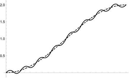
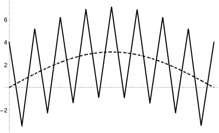
Figure 1: Graphical illustration of the instability of the solution to problem (2.3) with $F(t)=1-\cos\pi t$ and $n=3$. While $F$ and $\hat{F}_{n}$ (left, dotted and dashed respectively) and $f$ and $\hat{f}_{n}$ (right, dotted and dashed respectively) are basically indistinguishable when taking $\hat{f}_{0}=0$, the value $\hat{f}_{0}=4$ yields wildly oscillating functions $\hat{F}_{n}$ and $\hat{f}_{n}$ (solid lines).

Theorem 2.1.

For given $\hat{f}_{0}$, the coefficients $\{\vartheta^{(n)}_{m,k}\}$ solving problem (2.3) are given as follows. For $m=-1$, we have

$$\vartheta^{(n)}_{-1,0}=2^{n+2}\sum_{j=1}^{2^{n+1}}(-1)^{j}\left(F\Big{(}\frac{j}{2^{n+1}}\Big{)}-F\Big{(}\frac{j-1}{2^{n+1}}\Big{)}\right).$$

For $0\leq m\leq n-1$ and $0\leq k\leq 2^{m}-1$, we have

Finally, for $m=n$ and $0\leq k\leq 2^{n}-1$, we have

$$\begin{split}\vartheta^{(n)}_{n,k}&=-2^{n/2+2}\hat{f}_{0}-2^{3n/2+4}\sum_{j=1}^{2k}(-1)^{j}\left(F\Big{(}\frac{j}{2^{n+1}}\Big{)}-F\Big{(}\frac{j-1}{2^{n+1}}\Big{)}\right)\\ &+3\cdot 2^{3n/2+2}\left(F\Big{(}\frac{2k+1}{2^{n+1}}\Big{)}-F\Big{(}\frac{2k}{2^{n+1}}\Big{)}\right)-2^{3n/2+2}\left(F\Big{(}\frac{2k+2}{2^{n+1}}\Big{)}-F\Big{(}\frac{2k+1}{2^{n+1}}\Big{)}\right).\end{split}$$

The first observation we can make from Theorem 2.1 is that only the coefficients of the final generation, i.e., the numbers $\vartheta^{(n)}_{n,0},\dots,\vartheta^{(n)}_{n,2^{n}-1}$, depend on the initial value $\hat{f}_{0}$. Moreover, the formula for the final-generation coefficients $\vartheta^{(n)}_{n,0},\dots,\vartheta^{(n)}_{n,2^{n}-1}$ contains the additive term $-2^{n/2+2}\hat{f}_{0}$, which implies that any error made in estimating $\hat{f}_{0}$ translates into an additional $2^{n/2+2}$-fold error for each final-generation coefficient. In particular, the approximation errors $|\vartheta^{(n)}_{n,k}-\theta_{n,k}|$ can be made arbitrarily large by varying the initial condition $\hat{f}_{0}$. By contrast, all other Faber–Schauder coefficients, i.e., $\vartheta^{(n)}_{m,k}$ with $m\leq n-1$, are independent of $\hat{f}_{0}$. Thus, the instability with respect to $\hat{f}_{0}$ observed in Figure 1 arises exclusively from the coefficients $\vartheta^{(n)}_{n,0},\dots,\vartheta^{(n)}_{n,2^{n}-1}$ of the final generation.

Our second observation is the following counterintuitive phenomenon, which arises independently of the initial value $\hat{f}_{0}$. On the one hand, each estimated coefficient $\vartheta^{(n)}_{m,k}$ with $m\leq n-1$ is a linear combination of the values of $F$ over the grid $\mathbb{T}_{n+1}$ within the interval $[2^{-m\vee 0}k,2^{-m\vee 0}(k+1)]$, where $a\vee b$ is shorthand for $\max\{a,b\}$. This interval coincides with the support of the corresponding wavelet function $e_{m,k}$. By contrast, for $m=n$, the estimated coefficient $\vartheta^{(n)}_{n,k}$ involves all observations of $F$ within the interval $[0,2^{-n}(k+1)]$. This means that when approximating the derivative $f$ by the piecewise linear function $\hat{f}_{n}$, its behavior within $[2^{-n}k,2^{-n}(k+1)]$ is affected by values of $F$ potentially far away from that region. A graphical illustration of this phenomenon is presented in Figure 2, and a concrete computation will be given in Example 2.3. This nonlocal dependence of the coefficients $\vartheta^{(n)}_{n,k}$ on the observed data is counterintuitive and another cause for the instability of the quadratic spline interpolation.

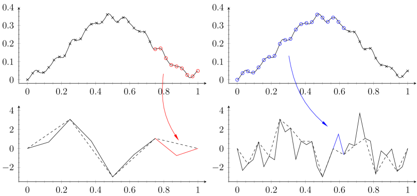
Figure 2: Graphical illustrations of the data dependence of the coefficients $\vartheta^{(n)}_{m,k}$. In the bottom-left graph, we plot the approximating functions $\hat{f}_{4,1}$ and $\hat{f}_{4,2}$ in dotted and solid lines respectively, and the contribution $\vartheta^{(4)}_{2,3}e_{2,3}$ is highlighted in red. In the bottom-right graph, we plot the approximating functions $\hat{f}_{4,3}$ and $\hat{f}_{4,4}$ in dotted and solid lines respectively, and the contribution $\vartheta^{(4)}_{4,9}e_{4,9}$ is highlighted in blue. Respective data points of the function $F$ that contribute to the estimation of $\vartheta^{(4)}_{2,3}$ and $\vartheta^{(4)}_{4,9}$ are highlighted by circles in the corresponding upper graphs. All data points that do not contribute to the computation of the coefficients in question are represented by cross marks.

In the following section, we will discover yet another issue with the final-generation Faber–Schauder coefficients of $\hat{f}_{n}$, which arises even if the true initial value $f(0)=F^{\prime}(0)$ is known, and $\hat{f}_{0}$ is set to that value. In this context, we will derive sharp upper and lower bounds on the approximation errors for the estimated Faber–Schauder coefficients up to generation $n-1$ and at generation $n$. That is, we will be looking at the Euclidean $\ell_{p}$-distances between the Faber–Schauder coefficients of $\hat{f}_{n}$ and the true Faber–Schauder coefficients of $f$ for $p\in\{1,2,\infty\}$ and under the assumption that $f(0)=F^{\prime}(0)$ is known. On the one hand, we will discover robust upper error bounds for the estimated Faber–Schauder coefficients up to generation $n-1$, which hold universally for each function $F\in C^{1}[0,1]$. On the other hand, we will see that $F\in C^{1}[0,1]$ can always be chosen in such a way that the error in generation $n$ exceeds the error up to generation $n-1$ by a factor of size $\mathcal{O}(2^{n})$ for the $\ell_{2}$- and $\ell_{1}$-norms and by a factor of size $\mathcal{O}(2^{n/2})$ for the $\ell_{\infty}$-norm. In Example 2.3, we will encounter an extreme case in which the approximation errors up to and including generation $n-1$ are all zero, while the error in generation $n$ can go to infinity even if the correct initial value $f(0)$ is known.

Conclusion. Our findings can informally be summarized as follows.

1. The estimated coefficients $\vartheta^{(n)}_{m,k}$ for $m\leq n-1$ are independent of the estimated initial value $\hat{f}_{0}$, and they admit robust error bounds for their convergence to the corresponding true Faber–Schauder coefficients of $f=F^{\prime}$.

2. By contrast, the final-generation coefficients $\vartheta^{(n)}_{n,0},\dots,\vartheta^{(n)}_{n,2^{n}-1}$ are strongly dependent on the estimated initial value $\hat{f}_{0}$. Even if the true initial value is known, they depend on $F$ in a nonlocal manner. Furthermore, the errors for their convergence to the corresponding true Faber–Schauder coefficients of $f=F^{\prime}$ are highly sensitive with respect to the function $F$.

Remark 2.2.

As mentioned in the introduction, the original motivation for this research stems from the problem of estimating the “roughness” of the function $f$. It was shown in [6, Theorem 2.4 and Proposition 4.1] that under mild assumptions on $f$,

$$\widehat{R}^{\ast}_{n}:=1-\frac{1}{n}\log_{2}\sqrt{\sum_{k=0}^{2^{n}-1}\theta^{2}_{n,k}}$$

is a strongly consistent statistical estimator for the so-called roughness exponent of $f$, provided that the true Faber–Schauder coefficients $\theta_{m,k}$ of $f$ are known. Thus, if, as in the case of volatility estimation [4], the function $f$ itself is unknown and only the values of its antiderivative $F$ are observed on the discrete grid $\mathbb{T}_{n+2}$, then our findings suggest to replace $\widehat{R}^{\ast}_{n}$ with the estimator

$$\widehat{\mathscr{R}}_{n}:=1-\frac{1}{n}\log_{2}\sqrt{\sum_{k=0}^{2^{n}-1}(\vartheta^{(n+1)}_{n,k}})^{2},$$

where the final-generation coefficients $\vartheta^{(n+1)}_{n+1,0},\dots,\vartheta^{(n+1)}_{n+1,2^{n+1}-1}$ are explicitly excluded from the computation. The statistical properties of $\widehat{\mathscr{R}}_{n}$ will be discussed in our follow-up paper [7].

We conclude this section with the following, computationally explicit example, in which the formulas from Theorem 2.1 recover the exact Faber–Schauder coefficients of $f$ up to and including generation $n-1$. In generation $n$, however, the estimated Faber–Schauder coefficients will differ from the true ones to the extent that their approximation errors may go to infinity even if the correct initial value $f(0)$ is known.

Example 2.3.

Consider the Takagi class, which was introduced by Hata and Yamaguti [8] and motivated by the celebrated, continuous but nowhere differentiable Takagi function. It consists of all functions of the following form:

$$f(t):=\sum_{m=0}^{\infty}c_{m}\phi(2^{m}t)=\sum_{m=0}^{\infty}2^{m/2}c_{m}\sum_{k=0}^{2^{m}-1}e_{m,k}(t),\quad\text{for}\quad t\in[0,1],$$ (2.5)

where $\{c_{m}\}_{m\in\mathbb{N}}$ is an absolutely summable sequence and $\phi(t):=\min_{z\in\mathbb{Z}}|t-z|$ denotes the tent map. The Takagi class has been studied intensively over the past decades; see, e.g., the surveys [1, 11]. Letting $F(t):=\int_{0}^{t}f(s)\,ds$ and $\hat{f}_{0}:=f(0)=0$, the coefficients solving (2.3) are given as follows,

$$\vartheta^{(n)}_{m,k}=\begin{cases}2^{m/2}c_{m}\quad&\text{for}\quad 0\leq m\leq n-1\quad\text{and}\quad 0\leq k\leq 2^{m}-1,\\ 2^{n/2}\sum_{m=n}^{\infty}c_{m}\quad&\text{for}\quad m=n\quad\text{and}\quad 0\leq k\leq 2^{n}-1.\end{cases}$$

The proof for these formulas is deferred to Section 4. It follows that up to and including generation $n-1$ the approximation error between all true and estimated Faber–Schauder coefficients is zero. For generation $n$, however, we have $|\vartheta^{(n)}_{n,k}-\theta_{n,k}|=2^{n/2}|\sum_{m=n+1}^{\infty}c_{m}|$. In particular, if the decay of $|\sum_{m=n+1}^{\infty}c_{m}|$ is slower than $O(2^{-n/2})$, then the approximation errors $|\vartheta^{(n)}_{n,k}-\theta_{n,k}|$ go to infinity as $n\uparrow\infty$.

2.2 Error analysis for the Faber–Schauder coefficients

In this section, we consider again functions $F\in C^{1}[0,1]$ with derivative $F^{\prime}=f$ and we suppose that $f(0)$ is known, so that we can set $\hat{f}_{0}:=f(0)$ in our problem (2.3). As a matter of fact, we may assume without loss of generality that $f(0)=\hat{f}_{0}=0$ and $F(0)=0$; otherwise we consider the function $F(t)-F(0)-f(0)t$, whose derivative has the same Faber–Schauder coefficients as $f$. We refer to [9] for a method for estimating $f(0)$ from the data $\{F(t):t\in\mathbb{T}_{n+1}\}$.

For studying the Euclidean $\ell_{p}$-norms of the approximation errors, it will be convenient to denote the Faber–Schauder coefficients of $f$ at or up to generation $m\geq-1$ by the respective column vectors $\bar{\bm{\theta}}_{m}$ and $\bm{\theta}_{m}$, i.e.,

$$\bar{\bm{\theta}}_{m}=\big{(}\theta_{m,0},\theta_{m,1}\cdots,\theta_{m,2^{m\vee 0}-1}\big{)}^{\top}\in\mathbb{R}^{2^{m\vee 0}}\quad\text{and}\quad\bm{\theta}_{m}=(\bar{\bm{\theta}}^{\top}_{-1},\bar{\bm{\theta}}^{\top}_{0},\cdots,\bar{\bm{\theta}}^{\top}_{m})^{\top}\in\mathbb{R}^{2^{m+1}}.$$ (2.6)

An analogous notation will be used for the coefficients in Theorem 2.1 solving (2.3). That is, for $-1\leq m\leq n$, we set

$$\bar{\bm{\vartheta}}^{(n)}_{m}=\big{(}\vartheta^{(n)}_{m,0},\vartheta^{(n)}_{m,1}\cdots,\vartheta^{(n)}_{m,2^{m\vee 0}-1}\big{)}^{\top}\in\mathbb{R}^{2^{m\vee 0}}\quad\text{and}\quad\bm{\vartheta}^{(n)}_{m}=((\bar{\bm{\vartheta}}^{(n)}_{-1})^{\top},(\bar{\bm{\vartheta}}^{(n)}_{0})^{\top},\cdots,(\bar{\bm{\vartheta}}^{(n)}_{m})^{\top})^{\top}\in\mathbb{R}^{2^{m+1}}.$$

Note that in particular $\bm{\vartheta}^{(n)}_{n}=\bm{\vartheta}^{(n)}$, and both notions will be used interchangeably in this paper. In this section, we study the approximation errors $\bm{\theta}_{m}-\bm{\vartheta}^{(n)}_{m}$ and $\bar{\bm{\theta}}_{m}-\bar{\bm{\vartheta}}^{(n)}_{m}$ by giving upper and lower bounds on their Euclidean $\ell_{p}$-norms for $p\in\{1,2,\infty\}$. These bounds will be given in terms of the $\ell_{p}$-norms of the $2^{n+1}$-dimensional column vector $\bm{z}_{n+1}:=(z^{(n+1)}_{1},\dots,z^{(n+1)}_{2^{n+1}})^{\top}$, where

$$z^{(n+1)}_{i}=2^{3(n+1)/2}\sum_{m=n+1}^{\infty}2^{-3m/2}\sum_{k=2^{m-n-1}(i-1)}^{2^{m-n-1}i-1}\theta_{m,k}\quad\text{for}\quad 1\leq i\leq 2^{n+1}.$$ (2.7)

The following criterion guarantees that the $\ell_{p}$-norm of $\bm{z}_{n+1}$ converges to zero as $n\uparrow\infty$. Combined with our subsequent error bounds, this proposition will yield a sufficient criterion for the convergence of the estimated Faber–Schauder coefficients to their true values.

Proposition 2.4.

Suppose that $f$ is continuously differentiable and that its derivative is Hölder continuous with exponent $\alpha\in(0,1]$. Then

$$\lVert{\bm{z}_{n+1}}\rVert_{\ell_{p}}=\begin{cases}\mathcal{O}(2^{-(n+1)(\alpha-\frac{1}{2})})&\quad\text{for}\quad p=1,\\ \mathcal{O}(2^{-(n+1)\alpha})&\quad\text{for}\quad p=2,\\ \mathcal{O}(2^{-(n+1)(\alpha+\frac{1}{2})})&\quad\text{for}\quad p=\infty.\\ \end{cases}$$ (2.8)

The following theorem gives sharp upper and lower bounds for the the $\ell_{2}$-norm of the approximation error $\bm{\vartheta}^{(n)}_{n-1}-\bm{\theta}_{n-1}$ of the estimated Faber–Schauder coefficients up to and including generation $n-1$.

Theorem 2.5.

The following assertions hold.

1. For arbitrary choice of $F$, we have

   $$\big{\lVert}{\bm{\vartheta}^{(n)}_{n-1}-\bm{\theta}_{n-1}}\big{\rVert}_{\ell_{2}}\leq\frac{1}{2}\lVert{\bm{z}_{n+1}}\rVert_{\ell_{2}}.$$ (2.9)

2. For each $\varepsilon>0$ and $-1\leq m\leq n-1$, the function $F$ can be chosen in such a way that

   $$\big{\lVert}{\bm{\vartheta}^{(n)}_{n-1}-\bm{\theta}_{n-1}}\big{\rVert}_{\ell_{2}}\geq\big{\lVert}{\bar{\bm{\vartheta}}^{(n)}_{m}-\bar{\bm{\theta}}_{m}}\big{\rVert}_{\ell_{2}}\geq(1-\varepsilon)\frac{1}{2}\lVert{\bm{z}_{n+1}}\rVert_{\ell_{2}}.$$

Our next results looks specifically at the error term $\|\bar{\bm{\vartheta}}^{(n)}_{n}-\bar{\bm{\theta}}_{n}\|_{\ell_{2}}$ for the Faber–Schauder coefficients of the $n^{\text{th}}$ generation.

Theorem 2.6.

For $n\geq 2$, the following assertions hold:

1. For arbitrary choice of $F$, we have

   $$\big{\lVert}{\bar{\bm{\vartheta}}^{(n)}_{n}-\bar{\bm{\theta}}_{n}}\big{\rVert}_{\ell_{2}}\leq\sqrt{2\left(1-\cos\frac{\pi}{2^{n+1}}\right)^{-1}+\frac{3}{4}}\cdot\lVert{\bm{z}_{n+1}}\rVert_{\ell_{2}}.$$ (2.10)

2. For each $\varepsilon>0$, the function $F$ can be chosen in such a way that

   $$\big{\lVert}{\bar{\bm{\vartheta}}^{(n)}_{n}-\bar{\bm{\theta}}_{n}}\big{\rVert}_{\ell_{2}}\geq(1-\varepsilon)\sqrt{2\left(1-\cos\frac{\pi}{2^{n+1}}\right)^{-1}-\frac{3}{4}}\cdot\lVert{\bm{z}_{n+1}}\rVert_{\ell_{2}}.$$ (2.11)

Since $1-\cos x\sim x^{2}/2$ as $x\downarrow 0$, the coefficients in (2.10) and (2.11) behave asymptotically as

$$\sqrt{2\left(1-\cos\frac{\pi}{2^{n+1}}\right)^{-1}\pm\frac{3}{4}}\sim\frac{2^{n+1}}{\pi}\quad\text{for}\quad n\uparrow\infty.$$ (2.12)

As a matter of fact, by combining the elementary inequality $1-\cos x\leq x^{2}/2$ with Theorem 2.5 (a) and Theorem 2.6 (b), we obtain the following corollary. As announced above, it states that the $\ell_{2}$-norm of the error in the final generation of the Faber–Schauder coefficients can be substantially larger than a factor of size $\mathcal{O}(2^{n})$ times the $\ell_{2}$-norm of the error of all previous generations combined. Moreover, it is worthwhile to point out that both vectors $\bar{\bm{\vartheta}}^{(n)}_{n}-\bar{\bm{\theta}}_{n}$ and $\bm{\vartheta}^{(n)}_{n-1}-\bm{\theta}_{n-1}$ are of length $2^{n}$.

Corollary 2.7.

For all $n\geq 2$ and $\varepsilon>0$, the function $F$ can be chosen in such a way that

$$\big{\lVert}{\bar{\bm{\vartheta}}^{(n)}_{n}-\bar{\bm{\theta}}_{n}}\big{\rVert}_{\ell_{2}}\geq 2(1-\varepsilon)\sqrt{\frac{2^{2n+2}}{\pi^{2}}-\frac{3}{4}}\big{\lVert}{\bm{\vartheta}^{(n)}_{n-1}-\bm{\theta}_{n-1}}\big{\rVert}_{\ell_{2}}.$$

Our bounds for the $\ell_{1}$- and $\ell_{\infty}$-norms, as stated in the following theorem, are even stronger than (2.10) and (2.11), because the constants for the upper and lower bounds are the same.

Theorem 2.8.

We fix $n\geq 2$ and let for $m=-1,0,\dots,n-1$ and $p\in\{1,\infty\}$,

$$\bar{c}_{p,m}:=\begin{cases}2^{\frac{m\vee 0-n-3}{2}}&\text{if $p=1$},\\ 2^{\frac{n-m\vee 0-1}{2}}&\text{if $p=\infty$},\end{cases}\qquad c_{p,m}:=\begin{cases}2^{-\frac{n+3}{2}}\big{(}\frac{2^{\frac{m+1}{2}}-1}{2^{1/2}-1}{\mathbbmss{1}}_{{}_{\scriptstyle\{m\geq 0\}}}+1\big{)}&\text{if $p=1$},\\ 2^{\frac{n-1}{2}}&\text{if $p=\infty$},\end{cases}$$

$$\bar{c}_{p,n}:=\begin{cases}2^{n+\frac{1}{2}}-2^{-3/2}&\text{if $p=1$},\\ 2^{n+\frac{3}{2}}-\sqrt{2}&\text{if $p=\infty$}.\end{cases}$$

Then the following assertions hold for $m=-1,0,\dots,n-1$ and $p\in\{1,.\infty\}$.

1. For arbitrary choice of $F$, we have $\|\bar{\bm{\vartheta}}^{(n)}_{m}-\bar{\bm{\theta}}_{m}\|_{\ell_{p}}\leq\bar{c}_{p,m}\lVert{\bm{z}_{n+1}}\rVert_{\ell_{p}}$, and for any given $\varepsilon>0$, the function $F$ can be chosen in such a way that $\|\bar{\bm{\vartheta}}^{(n)}_{m}-\bar{\bm{\theta}}_{m}\|_{\ell_{p}}>(1-\varepsilon)\bar{c}_{p,m}\lVert{\bm{z}_{n+1}}\rVert_{\ell_{p}}$.

2. For arbitrary choice of $F$, we have $\|{\bm{\vartheta}}^{(n)}_{m}-{\bm{\theta}}_{m}\|_{\ell_{p}}\leq c_{p,m}\lVert{\bm{z}_{n+1}}\rVert_{\ell_{p}}$, and for any given $\varepsilon>0$, the function $F$ can be chosen in such a way that $\|{\bm{\vartheta}}^{(n)}_{m}-{\bm{\theta}}_{m}\|_{\ell_{p}}>(1-\varepsilon)c_{p,m}\lVert{\bm{z}_{n+1}}\rVert_{\ell_{p}}$.

3. For arbitrary choice of $F$, we have $\|\bar{\bm{\vartheta}}^{(n)}_{n}-\bar{\bm{\theta}}_{n}\|_{\ell_{p}}\leq\bar{c}_{p,n}\cdot\lVert{\bm{z}_{n+1}}\rVert_{\ell_{p}}$, and for any given $\varepsilon>0$, the function $F$ can be chosen in such a way that $\|\bar{\bm{\vartheta}}^{(n)}_{n}-\bar{\bm{\theta}}_{n}\|_{\ell_{p}}>(1-\varepsilon)\bar{c}_{p,n}\lVert{\bm{z}_{n+1}}\rVert_{\ell_{p}}$.

4. For all $n\geq 2$ and $\varepsilon>0$, the function $F$ can be chosen in such a way that $\|\bar{\bm{\vartheta}}^{(n)}_{n}-\bar{\bm{\theta}}_{n}\|_{\ell_{p}}\geq(1-\varepsilon)\bar{c}_{p,n}c_{p,n-1}^{-1}\|{\bm{\vartheta}}^{(n)}_{n-1}-{\bm{\theta}}_{n-1}\|_{\ell_{p}}.$

Note that part (d) in the preceding theorem plays the role of Corollary 2.7 for the $\ell_{1}$- and $\ell_{\infty}$-norms and that the coefficients in that part satisfy

$$\frac{\bar{c}_{1,n}}{c_{1,n-1}}=\frac{\big{(}2^{n+\frac{1}{2}}-2^{-3/2}\big{)}}{2^{-\frac{n+3}{2}}\left(\frac{2^{n/2}-1}{2^{1/2}-1}+1\right)}\sim\big{(}\sqrt{2}-1\big{)}2^{n+2}\qquad\text{and}\qquad\frac{\bar{c}_{\infty,n}}{c_{\infty,n-1}}=\frac{2^{n+\frac{3}{2}}-\sqrt{2}}{2^{\frac{n-1}{2}}}\sim 2^{\frac{n}{2}+2}\qquad\text{as}\quad n\uparrow\infty.$$

Thus, for all $p\in\{1,2,\infty\}$, the ratio between $\|\bar{\bm{\vartheta}}^{(n)}_{n}-\bar{\bm{\theta}}_{n}\|_{\ell_{p}}$ and $\|{\bm{\vartheta}}^{(n)}_{n-1}-{\bm{\theta}}_{n-1}\|_{\ell_{p}}$ can become arbitrarily large as $n$ goes to infinity. This underscores our thesis that ${\bm{\vartheta}}^{(n)}_{n-1}$ is a more robust estimate for the true Faber–Schauder coefficients of $f$ than ${\bm{\vartheta}}^{(n)}_{n}$.

Theorems 2.5, 2.6, and 2.8 are actually corollaries to our results stated in Section 3. More specifically, they follow immediately from the equations (3.8) and (3.9) and Theorem 3.3.

2.3 Error analysis for the approximating functions

As discussed above, our analysis of the estimated Faber–Schauder coefficients suggests that dropping the final generation $\bar{\bm{\vartheta}}^{(n)}_{n}=(\vartheta^{(n)}_{n,0},\dots,\vartheta^{(n)}_{n,2^{n}-1})^{\top}$ of coefficients leads to a more robust estimate $\bm{\vartheta}^{(n)}_{n-1}$ of the true Faber–Schauder coefficients of $f$. A Faber–Schauder expansion based on these remaining coefficients should in turn lead to more robust approximations for the unknown functions $f$ and $F$. There is, however, a price to be paid for this robustness: the new approximating functions will no longer be interpolations of $f$ and $F$. That is, they may no longer coincide with $f$ and $F$ on the observation grid $\mathbb{T}_{n+1}$.

To analyze these induced approximating functions, we let again $F\in C^{1}[0,1]$ with $f=F^{\prime}$ and assume as in Section 2.2 that $F(0)=f(0)=0$. For $m=-1,0,\dots,n$, we then define

$$\hat{f}_{n,m}=\sum_{i=-1}^{m}\sum_{k=0}^{2^{i\vee 0}-1}\vartheta^{(n)}_{i,k}e_{i,k}\quad\text{and}\quad\hat{F}_{n,m}=\sum_{i=-1}^{m}\sum_{k=0}^{2^{i\vee 0}-1}\vartheta^{(n)}_{i,k}\psi_{i,k},$$ (2.13)

where the coefficients $\vartheta^{(n)}_{i,k}$ are as above. Then both $\hat{f}_{n,m}$ and the function $f_{m}$ defined in (2.1) will be piecewise linear with supporting grid $\mathbb{T}_{m+1}$.

Error analysis for quadratic spline interpolation has been well studied in the existing literature. Typically, results such as those in [14] are based on the mean-value theorem and provide error bounds for the $L_{\infty}[0,1]$-norm in terms of the first-order modulus of continuity of $f$. By contrast, our results presented here are based on the theorems in Section 2.2. They provide error bounds with respect to the $L_{p}[0,1]$-norms for $p\in\{1,2,\infty\}$ and in terms of the second-order modulus of continuity of $f$,

$$\omega_{2}(f,t):=\sup_{\begin{subarray}{c}\tau_{1},\tau_{2}\in[0,1]\\ |\tau_{1}-\tau_{2}|\leq t\end{subarray}}\left\{\left|f(\tau_{1})+f(\tau_{2})-2f\Big{(}\frac{\tau_{1}+\tau_{2}}{2}\Big{)}\right|\right\}.$$

Our results will involve the following constants, which we define for fixed $n\geq 2$,

$$\begin{split}A_{p}&:=\begin{cases}2^{-(n+3)/2}&\text{for $p=1$,}\\ 1/\sqrt{3}&\text{for $p=2$,}\\ 2^{(n+1)/2}&\text{for $p=\infty$,}\\ \end{cases}\qquad B_{p}:=\begin{cases}2^{n}&\text{for $p=1$,}\\ 2^{n+1}/\sqrt{3}&\text{for $p=2$,}\\ 2^{n+1}&\text{for $p=\infty$,}\\ \end{cases}\\ C_{p}&:=\begin{cases}2^{-(n+1)/2}&\text{for $p=1$,}\\ \gamma_{2}&\text{for $p=2$,}\\ 2^{(n+3)/2}&\text{for $p=\infty$,}\\ \end{cases}\qquad D_{p}:=\begin{cases}2^{n+1}&\text{for $p=1$,}\\ 2^{n+1}\gamma_{2}&\text{for $p=2$,}\\ 2^{n+2}&\text{for $p=\infty$,}\\ \end{cases}\end{split}$$ (2.14)

where

$$\gamma_{2}:=\frac{1}{\sqrt{3}}\bigg{(}1+2^{-n-1}\sqrt{2\Big{(}1-\cos\frac{\pi}{2^{n+1}}\Big{)}^{-1}+\frac{3}{4}}\bigg{)}.$$

Theorem 2.9.

The following inequalities hold for fixed $n\geq 2$, $0\leq m\leq n-1$, and $p\in\{1,2,\infty\}$,

$$\big{\lVert}{f_{m}-\hat{f}_{n,m}}\big{\rVert}_{L_{p}[0,1]} \leq A_{p}\lVert{\bm{z}_{n+1}}\rVert_{\ell_{p}}\leq B_{p}\sum_{k=n+1}^{\infty}\omega_{2}(f,2^{-k}),$$

$$\big{\lVert}{f_{n}-\hat{f}_{n,n}}\big{\rVert}_{L_{p}[0,1]} \leq C_{p}\lVert{\bm{z}_{n+1}}\rVert_{\ell_{p}}\leq D_{p}\sum_{k=n+1}^{\infty}\omega_{2}(f,2^{-k})$$

Remark 2.10.

Recall from (2.4) that $\lVert{\bm{z}_{n+1}}\rVert_{\ell_{p}}\to 0$ as $n\uparrow\infty$ if $f$ is continuously differentiable with Hölder continuous derivative. Thus, in this case, Theorem 2.9 yields that $\big{\lVert}{f_{m_{n}}-\hat{f}_{n,m_{n}}}\big{\rVert}_{L_{p}[0,1]}\to 0$ if $(m_{n})$ is any sequence with $m_{n}\leq n$.

Remark 2.11.

Theorem 2.9 gives error bounds between the truncated function $f_{m}$ and the approximation $\hat{f}_{n,m}$. Error bounds for $\lVert{f-\hat{f}_{n,m}}\rVert_{L_{p}[0,1]}$ can be obtained as follows. For instance, for $p=1$, we observe that $\lVert{e_{m,k}}\rVert_{L_{1}[0,1]}=2^{-3m/2-2}$ and $|\theta_{m,k}|\leq 2^{m/2}\omega_{2}(f,2^{-m})$. From here, it is easy to show that

$$\big{\lVert}{f-f_{m}}\big{\rVert}_{L_{1}[0,1]}\leq\frac{1}{4}\sum_{k=m+1}^{\infty}\omega_{2}(f,2^{-k}).$$

The desired error bound for $\lVert{f-\hat{f}_{n,m}}\rVert_{L_{1}[0,1]}$ can now be obtained in a straightforward manner from the triangle inequality and Theorem 2.9. Similar arguments also work in the cases of the $L_{2}$- and $L_{\infty}$-norms, where we can use that $\lVert{e_{m,k}}\rVert_{L_{2}[0,1]}=2^{-m-1}/{\sqrt{3}}$ and $\lVert{e_{m,k}}\rVert_{L_{\infty}[0,1]}=2^{-m/2-1}$. In the $L^{\infty}$-case, one can alternatively use the fact that $\lVert{f-f_{m}}\rVert_{L_{\infty}[0,1]}\leq 4\omega_{2}(f,2^{-m-1})$, which was established in [13, Theorem 1].

By combining the bounds explained in the preceding remark with the next theorem, one obtains bounds for the respective error $|F-\hat{F}_{n,n}|$ in various $L_{p}$-norms.

Theorem 2.12.

For $n\geq 2$, and $p\in\{1,2,\infty\}$, we have

$$\big{\lVert}{F-\hat{F}_{n,n}}\big{\rVert}_{L_{p}[0,1]}\leq a_{p}\big{\lVert}{f-\hat{f}_{n,n}}\big{\rVert}_{L_{p}[0,1]},$$

where $a_{1}=2^{-n-1}$, $a_{2}=2^{-n}/\pi$, and $a_{\infty}=2^{-n-2}$.

3 Matrix analysis of problem (2.3)

In this section, we present our approach to the proofs of the main results in this paper. It consists of a formulation of the problem (2.3) by means of linear algebra. To this end, consider the following wavelet system. We define $\psi_{-1,0}(t)=t^{2}/2$,

$$\psi_{0,0}(t)=\begin{cases}0&\quad t\in(-\infty,0),\\ \frac{1}{2}t^{2}&\quad t\in[0,\frac{1}{2}),\\ \frac{1}{4}-\frac{1}{2}(1-t)^{2}&\quad t\in[\frac{1}{2},1),\\ \frac{1}{4}&\quad t\in[1,\infty),\\ \end{cases}\quad\text{and}\quad\psi_{m,k}(t)=2^{-3m/2}\psi_{0,0}(2^{m}t-k)$$ (3.1)

for $m\in\mathbb{N}$ and $0\leq k\leq 2^{m}-1$.

Remark 3.1.

One easily verifies that $\int_{0}^{t}e_{m,k}(s)\,ds=\psi_{m,k}(t)$ for $m\geq-1$, $0\leq k\leq(2^{m}-1)\vee 0$, and $t\in\mathbb{R}$. Therefore, the fact that the Faber–Schauder functions are a Schauder basis of $C[0,1]$ implies that the collection of all functions $\psi_{m,k}$ augmented with $\{1,t\}$ forms a Schauder basis for the Banach space $C^{1}[0,1]$.

Using the functions $\{\psi_{m,k}\}$, we can transform the problem (2.3) into a standard linear equation. To this end, we assume again that $f(0)=0$ is known, that $\hat{f}_{0}=0$, and that $F(0)=0$; see the beginning of Section 2.2. We denote for $m\geq-1$ and ${k}\in\mathbb{N}$,

$$Q_{(m,k)}:=\left[\begin{array}[]{c c c c}\psi_{m,0}\Big{(}\frac{1}{2^{k}}\Big{)}&\psi_{m,1}\Big{(}\frac{1}{2^{k}}\Big{)}&\cdots&\psi_{m,2^{m\vee 0}-1}\Big{(}\frac{1}{2^{k}}\Big{)}\\ \psi_{m,0}\Big{(}\frac{2}{2^{k}}\Big{)}&\psi_{m,1}\Big{(}\frac{2}{2^{k}}\Big{)}&\cdots&\psi_{m,2^{m\vee 0}-1}\Big{(}\frac{2}{2^{k}}\Big{)}\\ \vdots&\vdots&\vdots&\vdots\\ \psi_{m,0}(1)&\psi_{m,1}(1)&\cdots&\psi_{m,2^{m\vee 0}-1}(1)\end{array}\\ \right]\in\mathbb{R}^{2^{k}\times 2^{m\vee 0}}.$$ (3.2)

Next, for $m,{k}\in\mathbb{N}$, we write

$$\Psi_{(m,{k})}=\Big{[}Q_{(-1,{k})},\cdots,Q_{(m,{k})}\Big{]}\in\mathbb{R}^{2^{{k}}\times 2^{m+1}}.$$ (3.3)

Remark 3.1 implies that $\Psi_{(m,{k})}$ has full rank. In particular, $\Psi_{n+1}:=\Psi_{(n,n+1)}\in\mathbb{R}^{2^{n+1}\times 2^{n+1}}$ is an invertible square matrix. We also use the shorthand notation

$$\bm{y}_{n+1}:=\left(F\Big{(}\frac{1}{2^{n+1}}\Big{)},F\Big{(}\frac{2}{2^{n+1}}\Big{)},\cdots,F(1)\right)^{\top}\in\mathbb{R}^{2^{n+1}}$$

for the values of $F$ over $\mathbb{T}_{n+1}$, our given data points. Using our assumptions $F(0)=0$ and $\hat{f}_{0}=0$, the problem (2.3) then becomes equivalent to the $2^{n+1}$-dimensional linear equation

$$\bm{\vartheta}^{(n)}=\Psi_{n+1}\bm{y}_{n+1},$$ (3.4)

in which the solution $\bm{\vartheta}^{(n)}$ describes the Faber–Schauder coefficients of $\hat{f}_{n}$ or, equivalently, the coefficients in the expansion of $\hat{F}_{n}$ in terms of the basis functions $\psi_{m,k}$.

It is a natural guess that the linear system (3.4) can be solved by a simple numerical inversion of the corresponding matrix $\Psi_{n+1}$. In practice, however, the numerical inversion of the matrix $\Psi_{n}$ becomes extremely unstable as the number of observation points increases; see Table 1. The main reason for this instability is the fact that matrix columns corresponding to neighboring wavelet functions become asymptotically co-linear. Fortunately, it is possible to algebraically invert the matrix $\Psi_{n}$. This inversion formula gives rise to an explicit solution of (3.4), which was stated in Theorem 2.1. The insight gained into the structure of $\Psi_{n}$ by deriving our inversion formula also forms the basis for our analysis of the approximation error. Our first lemma relates the two vectors $\bm{\vartheta}^{(n)}-\bm{\theta}_{n}$ and $\bm{z}_{n+1}$, where $\bm{z}_{n+1}$ was defined in (2.7), and $\bm{\theta}_{n}$ denotes as before the true Faber–Schauder coefficients of $f$ up to and including generation $n$.

Numerical values for $\log_{10}\det(\Psi_{n})$ for several values of $n$
$n$	2	3	4	5	6
$\log_{10}\det(\Psi_{n})$	-4.97	-13.4	-33.9	-82.03	-192.81

Table 1: Numerical values for $\log_{10}\det(\Psi_{n})$ for several values of $n$. Already for small values of $n$, the determinant of $\Psi_{n}$ is extremely small, which makes the problem (2.3) ill-posed from a numerical point of view.

Lemma 3.2.

For $n\in\mathbb{N}$, we set $P_{n}:=\Psi_{n+1}^{-1}Q_{(n+1,n+1)}$. Then $\bm{\vartheta}^{(n)}-\bm{\theta}_{n}=P_{n}\bm{z}_{n+1}$.

Proof. Remark 3.1 implies that $\bm{y}_{n+1}=\lim_{m\uparrow\infty}\Psi_{(m,n+1)}\bm{\theta}_{m}$. Thus, we have

$$\begin{split}\bm{\vartheta}^{(n)}&=\Psi^{-1}_{(n,n+1)}\bm{y}_{n+1}=\Psi^{-1}_{(n,n+1)}\lim_{m\uparrow\infty}\Psi_{(m,n+1)}\bm{\theta}_{m}\\ &=\lim_{m\uparrow\infty}\Psi_{(n,n+1)}^{-1}\Big{[}\Psi_{(n,n+1)},\,Q_{(n+1,n+1)},\,\cdots,\,Q_{(m,n+1)}\Big{]}\cdot\Big{[}\bm{\theta}^{\top}_{n},\bar{\bm{\theta}}^{\top}_{n+1},\cdots,\bar{\bm{\theta}}^{\top}_{m}\Big{]}^{\top}\\ &=\bm{\theta}_{n}+\Psi_{(n,n+1)}^{-1}\sum_{m=n+1}^{\infty}Q_{(m,n+1)}\bar{\bm{\theta}}_{m},\end{split}$$ (3.5)

where the third equality follows from (3.3). For $n\in\mathbb{N}$ and $m\geq n+1$, we define the $2^{n+1}\times 2^{m}$ dimensional matrix

$$U_{(m,n+1)}:=2^{(3n+3-3m)/2}\cdot\left[\begin{array}[]{c c c c }1\,1\,\cdots\,1&0\,0\,\cdots\,0&\cdots\cdots&0\,0\,\cdots\,0\\ 0\,0\,\cdots\,0&1\,1\,\cdots\,1&\cdots\cdots&0\,0\,\cdots\,0\\ \vdots&\vdots&\vdots&\vdots\\ \underbrace{0\,0\,\cdots\,0}_{2^{m-n-1}\text{ times}}&\underbrace{0\,0\,\cdots\,0}_{2^{m-n-1}\text{ times}}&\cdots\cdots&\underbrace{1\,1\,\cdots\,1}_{2^{m-n-1}\text{ times}}\\ \end{array}\right],$$

and by a simple matrix calculation, one can easily verify that

$$\bm{z}_{n+1}=\sum_{m=n+1}^{\infty}U_{(m,n+1)}\bar{\bm{\theta}}_{m}.$$ (3.6)

Moreover, for $m\geq n+1$, we have $\psi_{m,k}(2^{-(n+1)}j)=2^{-3m/2}\psi_{0,0}(2^{m-n-1}j-k)=0$ for $k\leq 2^{m-n-1}j$ and otherwise $2^{-3m/2-2}$. Thus, for $m\geq n+1$, the matrix $Q_{(m,n+1)}$ is of the following form:

$$Q_{(m,n+1)}=2^{-3m/2-2}\cdot\left[\begin{array}[]{c c c c }1\,1\,\cdots\,1&0\,0\,\cdots\,0&\cdots\cdots&0\,0\,\cdots\,0\\ 1\,1\,\cdots\,1&1\,1\,\cdots\,1&\cdots\cdots&0\,0\,\cdots\,0\\ \vdots&\vdots&\vdots&\vdots\\ \underbrace{1\,1\,\cdots\,1}_{2^{m-n-1}\text{ times}}&\underbrace{1\,1\,\cdots\,1}_{2^{m-n-1}\text{ times}}&\cdots\cdots&\underbrace{1\,1\,\cdots\,1}_{2^{m-n-1}\text{ times}}\\ \end{array}\right].$$ (3.7)

In particular, the matrix $Q_{(n+1,n+1)}$ is a lower triangular matrix that every non-zero entries are equal to one after proper scaling. Therefore, we get $Q_{(m,n+1)}=Q_{(n+1,n+1)}\cdot U_{(m,n+1)}$, this is because $Q_{(n+1,n+1)}$ can be regarded as a row operation acting on the matrix $U_{(m,n+1)}$ as a partial sum of rows. Applying this identity and (3.6) to (3.5) gives

$$\bm{\vartheta}^{(n)}-\bm{\theta}_{n}=\Psi_{(n,n+1)}^{-1}\sum_{m=n+1}^{\infty}Q_{(m,n+1)}\bar{\bm{\theta}}_{m}=P_{n}\sum_{m=n+1}^{\infty}U_{(m,n+1)}\bar{\bm{\theta}}_{m}=P_{n}\bm{z}_{n+1}.$$ ∎

Next, for any $-1\leq m\leq n$, the vectors $\bm{\vartheta}^{(n)}_{m}$ and $\bar{\bm{\vartheta}}^{(n)}_{m}$ are subvectors of $\bm{\vartheta}^{(n)}$, and we can represent them via simple linear transformations of $\bm{\vartheta}^{(n)}$. To this end, we denote for $-1\leq m\leq n$,

$$R^{(n)}_{m}:=\left[\bm{I}_{2^{m+1}\times 2^{m+1}},\bm{0}_{(2^{n+1}-2^{m+1})\times 2^{m+1}}\right]\quad\text{and}\quad\bar{R}^{(n)}_{m}:=\left[\bm{0}_{(2^{n+1}-2^{m\vee 0})\times 2^{m\vee 0}},\bm{I}_{2^{m\vee 0}\times 2^{m\vee 0}},\bm{0}_{(2^{n+1}-2^{m+1})\times 2^{m\vee 0}}\right],$$

where $\bm{I}_{m\times m}$ denotes the $m\times m$ dimensional identity matrix, and $\bm{0}_{m\times k}$ denotes the $m\times k$ dimensional zero matrix. Thus, $R^{(n)}_{m}$ is a $2^{m+1}\times 2^{n+1}$ dimensional matrix, and $R^{(n)}_{m}$ is a $2^{m\vee 0}\times 2^{n+1}$ dimensional matrix. Furthermore, one sees by means of a simple matrix manipulation that

$$\bm{\vartheta}^{(n)}_{m}-\bm{\theta}_{m}=R^{(n)}_{m}P_{n}\bm{z}_{n+1}\quad\text{and}\quad\bar{\bm{\vartheta}}^{(n)}_{m}-\bar{\bm{\theta}}_{m}=\bar{R}^{(n)}_{m}P_{n}\bm{z}_{n+1}.$$

It follows that for $p\in[1,\infty]$,

$$\big{\lVert}{\bm{\vartheta}^{(n)}_{m}-\bm{\theta}_{m}}\big{\rVert}_{\ell_{p}}\leq\lVert{R^{(n)}_{m}P_{n}}\rVert_{p}\lVert{\bm{z}_{n+1}}\rVert_{\ell_{p}},$$ (3.8)

where $\lVert{\cdot}\rVert_{p}$ denotes the $\ell_{p}$-induced operator norm for a matrix. Moreover, and for any $\varepsilon>0$, we can choose a vector $\bm{z}_{n+1}\in\mathbb{R}^{2^{n+1}}$ such that

$$\big{\lVert}{\bm{\vartheta}^{(n)}_{m}-\bm{\theta}_{m}}\big{\rVert}_{\ell_{p}}\geq(1-\varepsilon)\lVert{R^{(n)}_{m}P_{n}}\rVert_{p}\lVert{\bm{z}_{n+1}}\rVert_{\ell_{p}}.$$ (3.9)

Indeed, for any given vector $\bm{z}_{n+1}$, one can find Faber–Schauder coefficients $\theta_{m,k}$ that yield back $\bm{z}_{n+1}$ via (2.7); for instance we can take $\theta_{m,k}$ arbitrary for $m\leq n$, $\theta_{m,k}=0$ for $m\geq n+2$, and $\theta_{{n+1},k}=z^{(n+1)}_{k+1}$ for $k=0,\dots,2^{n+1}-1$. Thus, the Theorems 2.5 through 2.8 will follow immediately from corresponding bounds on the operator norm $\lVert{R^{(n)}_{m}P_{n}}\rVert_{p}$.

For the cases $p=1$ and $p=\infty$, the following result states exact expressions for this operator norm. For $p=2$, we have in part upper and lower bounds that are slightly different from each other.

Theorem 3.3.

For $n\in\mathbb{N}$, $-1\leq m\leq n$, and $p\in\{1,\infty\}$, $\lVert{\bar{R}^{(n)}_{m}P_{n}}\rVert_{p}=\bar{c}_{p,m}$ and $\lVert{R^{(n)}_{m}P_{n}}\rVert_{p}=c_{p,m}$, where the constants $\bar{c}_{p,m}$ and $c_{p,m}$ are as in Theorem 2.8. For $p=2$, we have $\lVert{\bar{R}^{(n)}_{m}P_{n}}\rVert_{2}=\lVert{R^{(n)}_{m}P_{n}}\rVert_{1}=\frac{1}{2}$ if $-1\leq m\leq n-1$, and for $m=n$ we have

$$\sqrt{2\left(1-\cos\frac{\pi}{2^{n+1}}\right)^{-1}-\frac{3}{4}}\leq\big{\lVert}{\bar{R}^{(n)}_{n}P_{n}}\big{\rVert}_{2}\leq\sqrt{2\left(1-\cos\frac{\pi}{2^{n+1}}\right)^{-1}+\frac{3}{4}}.$$

To prove results in Theorem 2.5, we first need an explicit representation of the matrix $P_{n}$. This is the content of the next lemma, whose proof will in turn require another lemma. Before stating it, though, we need to introduce some notation. For $m\geq 0$, we denote the column Rademacher vectors $\bm{r}^{+}_{m},\bm{r}^{-}_{m}\in\mathbb{R}^{2^{m}}$ by

$$\bm{r}^{+}_{m}=(\underbrace{-1,+1,-1,+1,\cdots,-1,+1}_{2^{m}\,\,\text{times}})^{\top}\quad\text{and}\quad\bm{r}^{-}_{m}=(\underbrace{+1,-1,+1,-1,\cdots,+1,-1}_{2^{m}\,\,\text{times}})^{\top}.$$ (3.10)

For given $n\in\mathbb{N}$ and $0\leq m\leq n-1$, we define the row vectors

$${\bm{\eta}}_{i,j}^{(m)}=\begin{cases}2^{\frac{m-n-3}{2}}\left((\bm{r}^{+}_{n-m})^{\top},\,(\bm{r}^{-}_{n-m})^{\top}\right)&\quad\text{for}\quad 1\leq i=j\leq 2^{m},\\ \bm{0}_{1\times 2^{n+1-m}}&\quad\text{for}\quad 1\leq i\neq j\leq 2^{m}.\end{cases}$$

We also define the column vectors $\bm{v}=(\frac{3}{2\sqrt{2}},\frac{-1}{2\sqrt{2}})$ and $\bm{u}=(\sqrt{2},-\sqrt{2})$. Then we define ${\mathscr{C}}_{-1},{\mathscr{C}}_{0},\dots,{\mathscr{C}}_{n}$ as follows. For $0\leq m\leq n-1$, we let

$${\mathscr{C}}_{m}:=\left[\begin{array}[]{c c c c c}{\bm{\eta}}^{(m)}_{1,1}&{\bm{\eta}}^{(m)}_{1,2}&\cdots&{\bm{\eta}}^{(m)}_{1,2^{m}-1}&{\bm{\eta}}^{(m)}_{1,2^{m}}\\ {\bm{\eta}}^{(m)}_{2,1}&{\bm{\eta}}^{(m)}_{2,2}&\cdots&{\bm{\eta}}^{(m)}_{2,2^{m}-1}&{\bm{\eta}}^{(m)}_{2,2^{m}}\\ \vdots&\vdots&\ddots&\vdots&\vdots\\ {\bm{\eta}}^{(m)}_{2^{m},1}&{\bm{\eta}}^{(m)}_{2^{m},2}&\cdots&{\bm{\eta}}^{(m)}_{2^{m},2^{m}-1}&{\bm{\eta}}^{(m)}_{2^{m},2^{m}}\\ \end{array}\right].$$ (3.11)

For $m=-1$ and $m=n$, we let

$${\mathscr{C}}_{-1}=2^{-\frac{n+3}{2}}(\bm{r}^{+}_{n+1})^{\top}\qquad\text{and}\qquad{\mathscr{C}}_{n}=\underbrace{\left[\begin{array}[]{c c c c c}\bm{v}&\bm{0}_{1\times 2}&\cdots&\bm{0}_{1\times 2}&\bm{0}_{1\times 2}\\ \bm{u}&\bm{v}&\cdots&\bm{0}_{1\times 2}&\bm{0}_{1\times 2}\\ \vdots&\vdots&\ddots&\vdots&\vdots\\ \bm{u}&\bm{u}&\cdots&\bm{v}&\bm{0}_{1\times 2}\\ \bm{u}&\bm{u}&\cdots&\bm{u}&\bm{v}\\ \end{array}\right]}_{2^{n}\text{ times}},$$

so that ${\mathscr{C}}_{m}\in\mathbb{R}^{2^{m\vee 0}\times 2^{n+1}}$ for $m=-1,\dots,n$.

Lemma 3.4.

The matrix $P_{n}$ is of the following form,

$$P_{n}=\left(({\mathscr{C}}_{-1})^{\top},({\mathscr{C}}_{0})^{\top},\cdots,({\mathscr{C}}_{n})^{\top}\right)^{\top}.$$ (3.12)

To prove Lemma 3.4, the following lemma is needed. For $n\in\mathbb{N}$ and $-1\leq m\leq n-1$, we define the column vector $\bm{w}^{+}_{(m,n)}\in\mathbb{R}^{2^{n-m}}$ and its reverse vector $\bm{w}^{-}_{(m,n)}\in\mathbb{R}^{2^{n-m}}$,

$$\bm{w}^{+}_{(m,n)}=\left(\frac{2k-1}{2^{(n-1-m\vee 0)/2}}\right)_{k=1,2,\cdots,2^{n-m}}\quad\text{and}\quad\bm{w}^{-}_{(m,n)}=\left(\frac{2k-1}{2^{(n-1-m\vee 0)/2}}\right)_{k=2^{n-m},\cdots,2,1}.$$ (3.13)

Lemma 3.5.

For given $n\in\mathbb{N}$ and $0\leq m\leq n$, we define the column vectors

$$\bm{\alpha}^{(m)}_{i,j}=\begin{cases}\big{(}(\bm{w}^{+}_{(m,n)})^{\top},(\bm{w}^{-}_{(m,n)})^{\top}\big{)}^{\top}&\quad\text{for}\quad 1\leq i=j\leq 2^{m},\\ \bm{0}_{2^{n-m+1}\times 1}&\quad\text{for}\quad 1\leq i\neq j\leq 2^{m}.\end{cases}$$

Then we define ${\mathscr{A}}_{-1},{\mathscr{A}}_{0},\cdots,{\mathscr{A}}_{n}$ as follows: For $0\leq m\leq n$, we let

$${\mathscr{A}}_{m}:=\left[\begin{array}[]{c c c c c}{\bm{\alpha}}^{(m)}_{1,1}&{\bm{\alpha}}^{(m)}_{1,2}&\cdots&{\bm{\alpha}}^{(m)}_{1,2^{m}-1}&{\bm{\alpha}}^{(m)}_{1,2^{m}}\\ {\bm{\alpha}}^{(m)}_{2,1}&{\bm{\alpha}}^{(m)}_{2,2}&\cdots&{\bm{\alpha}}^{(m)}_{2,2^{m}-1}&{\bm{\alpha}}^{(m)}_{2,2^{m}}\\ \vdots&\vdots&\ddots&\vdots&\vdots\\ {\bm{\alpha}}^{(m)}_{2^{m},1}&{\bm{\alpha}}^{(m)}_{2^{m},2}&\cdots&{\bm{\alpha}}^{(m)}_{2^{m},2^{m}-1}&{\bm{\alpha}}^{(m)}_{2^{m},2^{m}}\\ \end{array}\right]\in\mathbb{R}^{2^{n+1}\times 2^{m}}.$$ (3.14)

For $m=-1$, we set ${\mathscr{A}}_{-1}=\bm{\omega}^{+}_{(-1,n)}$, so that ${\mathscr{A}}_{m}\in\mathbb{R}^{2^{m\vee 0}\times 2^{n+1}}$ for $m=-1,\dots,n$. Then the matrix $A_{n}:=Q^{-1}_{(n+1,n+1)}\cdot\Psi_{n+1}$ is well-defined and of the following form

$$A_{n}=\big{(}{\mathscr{A}}_{-1},{\mathscr{A}}_{0},\cdots,{\mathscr{A}}_{n}\big{)}.$$

Proof.

The proof has two steps. First, we claim and show that $Q_{(n+1,n+1)}$ is invertible and

$$Q^{-1}_{(n+1,n+1)}=2^{\frac{3(n+1)}{2}+2}\left[\begin{array}[]{c c c c c }1&0&\cdots&0&0\\ -1&1&\cdots&0&0\\ 0&-1&\cdots&0&0\\ \vdots&\vdots&\ddots&\vdots&\vdots\\ 0&0&\cdots&-1&1\\ \end{array}\right].$$ (3.15)

Taking $m=n+1$ in (3.7) implies that $Q_{(n+1,n+1)}$ is of the form

$$Q_{(n+1,n+1)}=2^{-\frac{3(n+1)}{2}-2}\left[\begin{array}[]{c c c c c }1&0&\cdots&0&0\\ 1&1&\cdots&0&0\\ \vdots&\vdots&\ddots&\vdots&\vdots\\ 1&1&\cdots&1&0\\ 1&1&\cdots&1&1\\ \end{array}\right],$$

and thus, we only need to show that

$$\left[\begin{array}[]{c c c c c }1&0&\cdots&0&0\\ -1&1&\cdots&0&0\\ 0&-1&\cdots&0&0\\ \vdots&\vdots&\ddots&\vdots&\vdots\\ 0&0&\cdots&-1&1\\ \end{array}\right]\left[\begin{array}[]{c c c c c }1&0&\cdots&0&0\\ 1&1&\cdots&0&0\\ \vdots&\vdots&\ddots&\vdots&\vdots\\ 1&1&\cdots&1&0\\ 1&1&\cdots&1&1\\ \end{array}\right]=\bm{I}_{2^{n+1}\times 2^{n+1}},$$

The above identity indeed holds for the following reason: The first matrix can be regarded as a row operation acting on the subsequent lower triangular matrix by subtracting preceding rows. To be more specific, for $n\in\mathbb{N}$, the $n^{\text{th}}$ row of the second matrix consists of ones at its first $n$ positions and zeros at the remaining position. The difference of the $n^{\text{th}}$ and the $(n-1)^{\text{th}}$ row then only has a one at the $n^{\text{th}}$ position and zeros elsewhere. This then leads to

$$A_{n}=Q^{-1}_{(n+1,n+1)}\Psi_{(n,n+1)}=\Big{(}Q^{-1}_{(n+1,n+1)}Q_{(-1,n+1)},Q^{-1}_{(n+1,n+1)}Q_{(0,n+1)}\cdots,Q^{-1}_{(n+1,n+1)}Q_{(n,n+1)}\Big{)}.$$

Again, the matrix $Q^{-1}_{(n+1,n+1)}$ acts on each matrix $Q_{(m,n+1)}$ by subtracting preceding rows after proper scaling. For instance, the first column of the matrix $Q^{-1}_{(n+1,n+1)}Q_{(m,n+1)}$ becomes

$$2^{3(n+1)/2+2}\left(\psi_{m,0}\Big{(}\frac{1}{2^{n+1}}\Big{)},\psi_{m,0}\Big{(}\frac{2}{2^{n+1}}\Big{)}-\psi_{m,0}\Big{(}\frac{1}{2^{n+1}}\Big{)},\cdots,\psi_{m,0}(1)-\psi_{m,0}\Big{(}\frac{2^{n+1}-1}{2^{n+1}}\Big{)}\right)^{\top}.$$ (3.16)

Note that

$$\begin{split}\psi_{m,0}\Big{(}\frac{k}{2^{n+1}}\Big{)}&-\psi_{m,0}\Big{(}\frac{k-1}{2^{n+1}}\Big{)}=2^{-3m/2}\left(\psi_{0,0}\Big{(}\frac{k}{2^{n-m+1}}\Big{)}-\psi_{0,0}\Big{(}\frac{k-1}{2^{n-m+1}}\Big{)}\right)\\ &=\begin{cases}2^{m/2-2n-3}(2k-1)&\quad\text{for $1\leq k\leq 2^{n-m}$,}\\ 2^{m/2-2n-3}\left(2^{n-m+2}-(2k-1)\right)&\quad\text{for $2^{n-m}+1\leq k\leq 2^{n-m+1}$,}\\ 0&\quad\text{otherwise.}\end{cases}\end{split}$$ (3.17)

Hence, (3.16) and (3.17) demonstrate that the first column fits into the form (3.14). Furthermore, by translation, this assertion carries over to all columns of the matrix $Q^{-1}_{(n+1,n+1)}Q_{(m,n+1)}$ for $m\geq 0$. For the case $m=-1$, we have

$$Q^{-1}_{(n+1,n+1)}Q_{(-1,n+1)}=2^{3(n+1)/2+1}\left(\Big{(}\frac{1}{2^{n+1}}\Big{)},\Big{(}\frac{2}{2^{n+1}}\Big{)}^{2}-\Big{(}\frac{1}{2^{n+1}}\Big{)}^{2},\cdots,1-\Big{(}\frac{2^{n+1}-1}{2^{n+1}}\Big{)}^{2}\right)^{\top}.$$

Since for any $1\leq k\leq 2^{n+1}$, we have

$$2^{3(n+1)/2+1}\left(\frac{(k-1)^{2}}{2^{2n+2}}-\frac{k^{2}}{2^{2n+2}}\right)=2^{-n/2+1/2}(2k-1),$$

thus, $Q^{-1}_{(n+1,n+1)}Q_{(-1,n+1)}=\bm{\omega}^{+}_{(-1,n)}$. This completes the proof. ∎

Now we can proceed to proving Lemma 3.4.

Proof of Lemma 3.4.

For $n\in\mathbb{N}$, let $A_{n}$ be defined as in (3.14). Since $A_{n}$ is of full-rank, it suffices to show that $L_{n}:=P_{n}A_{n}$ is equal to $\bm{I}_{2^{n+1}\times 2^{n+1}}$. We have

$$\begin{split}L_{n}&=\left[\begin{array}[]{c c c c}{\mathscr{C}}_{-1}{\mathscr{A}}_{-1}&{\mathscr{C}}_{-1}{\mathscr{A}}_{0}&\cdots&{\mathscr{C}}_{-1}{\mathscr{A}}_{n}\\ {\mathscr{C}}_{0}{\mathscr{A}}_{-1}&{\mathscr{C}}_{0}{\mathscr{A}}_{0}&\cdots&{\mathscr{C}}_{0}{\mathscr{A}}_{n}\\ \vdots&\vdots&\ddots&\vdots\\ {\mathscr{C}}_{n}{\mathscr{A}}_{-1}&{\mathscr{C}}_{n}{\mathscr{A}}_{0}&\cdots&{\mathscr{C}}_{n}{\mathscr{A}}_{n}\\ \end{array}\right]=:\left[\begin{array}[]{c c c c }{\mathscr{L}}_{(-1,-1)}&{\mathscr{L}}_{(-1,0)}&\cdots&{\mathscr{L}}_{(-1,n)}\\ {\mathscr{L}}_{(0,-1)}&{\mathscr{L}}_{(0,0)}&\cdots&{\mathscr{L}}_{(0,n)}\\ \vdots&\vdots&\ddots&\vdots\\ {\mathscr{L}}_{(n,-1)}&{\mathscr{L}}_{(n,0)}&\cdots&{\mathscr{L}}_{(n,n)}\\ \end{array}\right],\end{split}$$

where ${\mathscr{L}}_{(m,k)}:={\mathscr{C}}_{m}{\mathscr{A}}_{k}\in\mathbb{R}^{2^{m\vee 0}\times 2^{k\vee 0}}$ for $-1\leq m,k\leq n$. Now, we only need to show that ${\mathscr{L}}_{(m,k)}=\bm{0}_{2^{m\vee 0}\times 2^{k\vee 0}}$ and ${\mathscr{L}}_{(m,m)}=\bm{I}_{2^{m\vee 0}\times 2^{m\vee 0}}$ for $-1\leq m\neq k\leq n$.

First, we show that that ${\mathscr{L}}_{(m,m)}=\bm{I}_{2^{m}\times 2^{m}}$ for $0\leq m\leq n-1$. To this end,

$$\begin{split}{\mathscr{L}}_{(m,m)}&=\left[\begin{array}[]{c c c c}{\bm{\eta}}^{(m)}_{1,1}&{\bm{\eta}}^{(m)}_{1,2}&\cdots&{\bm{\eta}}^{(m)}_{1,2^{m}}\\ {\bm{\eta}}^{(m)}_{2,1}&{\bm{\eta}}^{(m)}_{2,2}&\cdots&{\bm{\eta}}^{(m)}_{2,2^{m}}\\ \vdots&\vdots&\ddots&\vdots\\ {\bm{\eta}}^{(m)}_{2^{m},1}&{\bm{\eta}}^{(m)}_{2^{m},2}&\cdots&{\bm{\eta}}^{(m)}_{2^{m},2^{m}}\\ \end{array}\right]\left[\begin{array}[]{c c c c }{\bm{\alpha}}^{(m)}_{1,1}&{\bm{\alpha}}^{(m)}_{1,2}&\cdots&{\bm{\alpha}}^{(m)}_{1,2^{m}}\\ {\bm{\alpha}}^{(m)}_{2,1}&{\bm{\alpha}}^{(m)}_{2,2}&\cdots&{\bm{\alpha}}^{(m)}_{2,2^{m}}\\ \vdots&\vdots&\ddots&\vdots\\ {\bm{\alpha}}^{(m)}_{2^{m},1}&{\bm{\alpha}}^{(m)}_{2^{m},2}&\cdots&{\bm{\alpha}}^{(m)}_{2^{m},2^{m}}\\ \end{array}\right]=:\left[\begin{array}[]{c c c c}\ell^{(m)}_{1,1}&\ell^{(m)}_{1,2}&\cdots&\ell^{(m)}_{1,2^{m}}\\ \ell^{(m)}_{2,1}&\ell^{(m)}_{2,2}&\cdots&\ell^{(m)}_{2,2^{m}}\\ \vdots&\vdots&\ddots&\vdots\\ \ell^{(m)}_{2^{m},1}&\ell^{(m)}_{2^{m},2}&\cdots&\ell^{(m)}_{2^{m},2^{m}}\\ \end{array}\right],\end{split}$$

where $\ell^{(m)}_{i,j}=\sum_{k=1}^{2^{m}}{\bm{\eta}}^{(m)}_{i,k}{\bm{\alpha}}^{(m)}_{k,j}$. Since ${\bm{\eta}}^{(m)}_{i,j}=\bm{0}_{1\times 2^{n+1-m}}$ and ${\bm{\alpha}}^{(m)}_{i,j}=\bm{0}_{2^{n+1-m}\times 1}$ for $i\neq j$, therefore $\ell^{(m)}_{i,j}=0$ for $i\neq j$. Moreover, we get in the same way that

$$\begin{split}\ell^{(m)}_{i,i}&={\bm{\eta}}^{(m)}_{i,i}{\bm{\alpha}}^{(m)}_{i,i}=2^{(m-n-3)/2}\left((\bm{r}^{+}_{n-m})^{\top}\bm{w}^{+}_{(m,n)}+(\bm{r}^{-}_{n-m})^{\top}\bm{w}^{-}_{(m,n)}\right)\\ &=2^{m-n-1}\left(\sum_{k=1}^{2^{n-m}}(-1)^{k}(2k-1)+\sum_{k=2^{n-m+1}}^{2^{n-m+1}}(-1)^{k+1}\left(2^{n-m+2}-(2k-1)\right)\right)\\ &=2^{m-n}\sum_{k=1}^{2^{n-m}}(-1)^{k}(2k-1)=2^{m-n}\sum_{k=1}^{2^{n-m-1}}2=1.\end{split}$$

Next, for the case $m=-1$, we prove analogously that

$${\mathscr{C}}_{-1}{\mathscr{A}}_{-1}=2^{-\frac{n+3}{2}}(\bm{r}^{+}_{n+1})^{\top}\bm{w}^{+}_{(-1,n)}=2^{-n-1}\left(\sum_{k=1}^{2^{n+1}}(-1)^{k}(2k-1)\right)=1.$$

Last, it follows that

$${\mathscr{C}}_{n}{\mathscr{A}}_{n}=2^{1/2}\left[\begin{array}[]{ccccccc}\frac{3}{2\sqrt{2}}&-\frac{1}{2\sqrt{2}}&0&0&\cdots&0&0\\ \sqrt{2}&-\sqrt{2}&\frac{3}{2\sqrt{2}}&-\frac{1}{2\sqrt{2}}&\cdots&0&0\\ \vdots&\vdots&\vdots&\vdots&\ddots&\vdots&\vdots\\ \sqrt{2}&-\sqrt{2}&\sqrt{2}&-\sqrt{2}&\cdots&\frac{3}{2\sqrt{2}}&-\frac{1}{2\sqrt{2}}\\ \end{array}\right]\left[\begin{array}[]{cccc}1&0&\cdots&0\\ 1&0&\cdots&0\\ 0&1&\cdots&0\\ 0&1&\cdots&0\\ \vdots&\vdots&\vdots&\vdots\\ 0&0&\cdots&1\\ 0&0&\cdots&1\\ \end{array}\right]=\bm{I}_{2^{n}\times 2^{n}}.$$

The above identity holds, because the second matrix can be regarded as a column operation acting on the first matrix by adding subsequent columns. To be more specific, for $1\leq m\leq 2^{n}$, the $m^{\text{th}}$ column of the matrix ${\mathscr{L}}_{(n,n)}$ equals the sum of the $(2m-1)^{\text{th}}$ and the $(2m)^{\text{th}}$ columns of ${\mathscr{C}}_{n}$. Prior to the $m^{\text{th}}$ entry, each entry of the $(2m-1)^{\text{th}}$ and the $(2m)^{\text{th}}$ column of ${\mathscr{C}}_{n}$ equals zero and all entries are equal to $\pm\sqrt{2}$ afterwards respectively. Thus, it is clear that ${\mathscr{C}}_{n}{\mathscr{A}}_{n}=\bm{I}_{2^{n}\times 2^{n}}$.

Next, we are going to show that ${\mathscr{L}}_{(m,k)}=\bm{0}_{2^{m}\times 2^{k}}$ for $0\leq m\neq k\leq n-1$, and we first show this holds with $m<k$. Under this assumption, we have

$$\begin{split}{\mathscr{C}}_{m}{\mathscr{A}}_{k}&=\left[\begin{array}[]{c c c c}{\bm{\eta}}^{(m)}_{1,1}&\bm{0}_{1\times 2^{n+1-m}}&\cdots&\bm{0}_{1\times 2^{n+1-m}}\\ \bm{0}_{1\times 2^{n+1-m}}&{\bm{\eta}}^{(m)}_{2,2}&\cdots&\bm{0}_{1\times 2^{n+1-m}}\\ \vdots&\vdots&\ddots&\vdots\\ \bm{0}_{1\times 2^{n+1-m}}&\bm{0}_{1\times 2^{n+1-m}}&\cdots&{\bm{\eta}}^{(m)}_{2^{m},2^{m}}\\ \end{array}\right]\left[\begin{array}[]{c c c c}{\bm{\alpha}}^{(k)}_{1,1}&\bm{0}_{2^{n+1-k}\times 1}&\cdots&\bm{0}_{2^{n+1-k}\times 1}\\ \bm{0}_{2^{n+1-k}\times 1}&{\bm{\alpha}}^{(k)}_{2,2}&\cdots&\bm{0}_{2^{n+1-k}\times 1}\\ \vdots&\vdots&\ddots&\vdots\\ \bm{0}_{2^{n+1-k}\times 1}&\bm{0}_{2^{n+1-k}\times 1}&\cdots&{\bm{\alpha}}^{(k)}_{2^{k},2^{k}}\\ \end{array}\right]\\ &=\left[\begin{array}[]{c c c c}{\bm{\eta}}^{(m)}_{1,1}{\bm{\alpha}}^{(m,k)}_{1,1}&\bm{0}_{1\times 2^{k-m}}&\cdots&\bm{0}_{1\times 2^{k-m}}\\ \bm{0}_{1\times 2^{k-m}}&{\bm{\eta}}^{(m)}_{2,2}{\bm{\alpha}}^{(m,k)}_{2,2}&\cdots&\bm{0}_{1\times 2^{k-m}}\\ \vdots&\vdots&\ddots&\vdots\\ \bm{0}_{1\times 2^{k-m}}&\bm{0}_{1\times 2^{k-m}}&\cdots&{\bm{\eta}}^{(m)}_{2^{m},2^{m}}{\bm{\alpha}}^{(m,k)}_{2^{m},2^{m}}\\ \end{array}\right],\end{split}$$

where the $2^{n+m-1}\times 2^{k-m}$ dimensional matrix ${\bm{\alpha}}^{(m,k)}_{i,i}$ is defined as

$${\bm{\alpha}}^{(m,k)}_{i,i}:=\left[\begin{array}[]{c c c c}{\bm{\alpha}}^{(k)}_{1,1}&\bm{0}_{2^{n+1-k}\times 1}&\cdots&\bm{0}_{2^{n+1-k}\times 1}\\ \bm{0}_{2^{n+1-k}\times 1}&{\bm{\alpha}}^{(k)}_{2,2}&\cdots&\bm{0}_{2^{n+1-k}\times 1}\\ \vdots&\vdots&\ddots&\vdots\\ \bm{0}_{2^{n+1-k}\times 1}&\bm{0}_{2^{n+1-k}\times 1}&\cdots&{\bm{\alpha}}^{(k)}_{2^{k-m},2^{k-m}}\\ \end{array}\right],$$

for any $1\leq i\leq 2^{m}$. Further calculation yields that for each $1\leq i\leq 2^{m}$,

$$\begin{split}&{\bm{\eta}}^{(m)}_{i,i}{\bm{\alpha}}^{(m,k)}_{i,i}=2^{(m-n-3)/2}\left((\bm{r}^{+}_{n-m})^{\top},(\bm{r}^{-}_{n-m})^{\top}\right)\left[\begin{array}[]{c c c c}{\bm{\alpha}}^{(k)}_{1,1}&\bm{0}_{2^{n-k+1}\times 1}&\cdots&\bm{0}_{2^{n-k+1}\times 1}\\ \bm{0}_{2^{n-k+1}\times 1}&{\bm{\alpha}}^{(k)}_{2,2}&\cdots&\bm{0}_{2^{n-k+1}\times 1}\\ \vdots&\vdots&\vdots&\vdots\\ \bm{0}_{2^{n-k+1}\times 1}&\bm{0}_{2^{n-k+1}\times 1}&\cdots&{\bm{\alpha}}^{(k)}_{2^{k-m},2^{k-m}}\\ \end{array}\right]\\ &=2^{(m-n-3)/2}\big{(}\underbrace{(\bm{r}_{n-k}^{+})^{\top},\cdots,(\bm{r}_{n-k}^{+})^{\top}}_{2^{k-m}\text{ times}},\,\,\underbrace{(\bm{r}_{n-k}^{-})^{\top},\cdots,(\bm{r}_{n-k}^{-})^{\top}}_{2^{k-m}\text{ times}}\big{)}\left[\begin{array}[]{c c c c}\bm{w}^{+}_{(k,n)}&\bm{0}_{2^{n-k}\times 1}&\cdots&\bm{0}_{2^{n-k}\times 1}\\ \bm{w}^{-}_{(k,n)}&\bm{0}_{2^{n-k}\times 1}&\cdots&\bm{0}_{2^{n-k}\times 1}\\ \bm{0}_{2^{n-k}\times 1}&\bm{w}^{+}_{(k,n)}&\cdots&\bm{0}_{2^{n-k}\times 1}\\ \bm{0}_{2^{n-k}\times 1}&\bm{w}^{-}_{(k,n)}&\cdots&\bm{0}_{2^{n-k}\times 1}\\ \vdots&\vdots&\vdots&\vdots\\ \bm{0}_{2^{n-k}\times 1}&\bm{0}_{2^{n-k}\times 1}&\cdots&\bm{w}^{+}_{(k,n)}\\ \bm{0}_{2^{n-k}\times 1}&\bm{0}_{2^{n-k}\times 1}&\cdots&\bm{w}^{-}_{(k,n)}\\ \end{array}\right]\\ &=2^{(m-n-3)/2}\big{(}\underbrace{(\bm{r}_{n-k}^{+})^{\top}(\bm{w}^{+}_{(k,n)}+\bm{w}^{-}_{(k,n)}),\cdots}_{2^{k-m-1}\text{ times}},\,\,\underbrace{(\bm{r}_{n-k}^{-})^{\top}(\bm{w}^{+}_{(k,n)}+\bm{w}^{-}_{(k,n)}),\cdots}_{2^{k-m-1}\text{ times}}\big{)}.\end{split}$$

Since $\bm{w}^{+}_{(k,n)}+\bm{w}^{-}_{(k,n)}=2^{\frac{m-n+1}{2}}\big{(}(2^{n-m+1}-1)+1\big{)}\cdot\bm{1}_{2^{n-k}\times 1}=2^{\frac{n-m+3}{2}}\cdot\bm{1}_{2^{n-k}\times 1}$, it follows that

$$(\bm{r}_{n-k}^{+})^{\top}(\bm{w}^{+}_{(k,n)}+\bm{w}^{-}_{(k,n)})=(\bm{r}_{n-k}^{-})^{\top}(\bm{w}^{+}_{(k,n)}+\bm{w}^{-}_{(k,n)})=0.$$ (3.18)

Thus, we have ${\bm{\eta}}^{(m)}_{i,i}{\bm{\alpha}}^{(m,k)}_{i,i}=\bm{0}_{1\times 2^{k-m}}$, and hence, ${\mathscr{L}}_{(m,k)}=\bm{0}_{2^{m}\times 2^{k}}$. Since the matrices $A_{n}$ and $P_{n}$ are symmetric by construction, we have ${\mathscr{L}}_{(m,k)}={\mathscr{L}}_{(k,m)}^{\top}=\bm{0}_{2^{k}\times 2^{m}}$ for $m>k$. This now proves our claim ${\mathscr{L}}_{(m,k)}=\bm{0}_{2^{m}\times 2^{k}}$ for $0\leq m\neq k\leq n-1$.

For the case $m=-1$, we get in the same manner that for $-1\leq k\leq n-1$,

$${\mathscr{C}}_{-1}{\mathscr{A}}_{k}=2^{-\frac{n+3}{2}}\big{(}\underbrace{(\bm{r}_{n-k}^{+})^{\top}(\bm{w}^{+}_{(k,n)}+\bm{w}^{-}_{(k,n)}),\cdots,(\bm{r}_{n-k}^{+})^{\top}(\bm{w}^{+}_{(k,n)}+\bm{w}^{-}_{(k,n)}}_{2^{k}\text{ times}}\big{)}=\bm{0}_{1\times 2^{k}}.$$

Finally, for $-1\leq m\leq n-1$, recall that we denote the $(i,j)$-entry of ${\mathscr{L}}_{(n,m)}$ by $\ell^{(n,m)}_{i,j}$. A simple matrix calculation implies that

$$\ell^{(n,m)}_{i,j}=(\underbrace{\bm{u},\cdots,\bm{u}}_{i\,\,\text{times}},\,\bm{v},\,\underbrace{\bm{0}_{1\times 2},\,\cdots,\,\bm{0}_{1\times 2}}_{2^{n}-i-1\,\,\text{times}})\big{(}\underbrace{\bm{0}_{1\times 2^{n-m}},\cdots}_{2j\,\,\text{times}},(\bm{w}^{+}_{(m,n)})^{\top},(\bm{w}^{-}_{(m,n)})^{\top},\cdots,\underbrace{\bm{0}_{1\times 2^{n-m}},\cdots}_{2^{m+1}-2j-2\,\,\text{times}}\big{)}^{\top}.$$

The fact that

$$\underbrace{(\bm{u},\cdots,\bm{u})}_{2^{n-m-1}\,\,\text{times}}\bm{w}^{\pm}_{(m,n)}=\sqrt{2}\cdot(\bm{r}^{+}_{n-m})^{\top}\bm{w}^{\pm}_{(m,n)}=0.$$

directly yields that $\ell^{(n,m)}_{i,j}=0$ for $i\geq 2^{n-m}(j+1)$. Otherwise, for $i\leq 2^{n-m}j-1$, we clearly have $\ell_{i,j}^{(n,m)}=0$, as every non-zero vector must by multiplied by a zero vector. For $2^{n-m}j\leq i\leq 2^{n-m-1}(2j+1)-1$, we denote $\tau=i-2^{n-m}j$. Then a matrix calculation gives

$$\begin{split}\ell^{(n,m)}_{i,j}&=\frac{\sqrt{2}}{2^{(n+3-m)/2}}\left(\sum_{k=1}^{\tau}(-1)^{k}(2k-1)+\frac{3}{4}(2\tau+1)-\frac{1}{4}(2\tau+3)\right)\\ &=\frac{\sqrt{2}}{2^{2n-m/2-1}}(\tau-\frac{3}{4}(2\tau+1)-\frac{1}{4}(2\tau+3))=0.\end{split}$$

The case $2^{n-m-1}(2j+1)\leq i\leq 2^{n-m}(j+1)-1$ can be proved analogously using the symmetry property of $\bm{w}^{\pm}_{(m,n)}$ for $m\geq 0$. For the case $m=-1$, one can easily apply the same method to obtain ${\mathscr{L}}_{(n,-1)}=\bm{0}_{2^{n+1}\times 1}$. This completes the proof. ∎

Next, we shall apply Lemma 3.4 to obtain the matrix norms of $\bar{R}^{(n)}_{m}P_{n}$ and $R^{(n)}_{m}P_{n}$ as stated in Theorem 3.3. We give separate proofs for the cases $p=\infty$, $p=1$, and $p=2$. Recall that for an $m\times n$ matrix $A=(a_{ij})$, we have $\lVert{A}\rVert_{1}=\max_{1\leq j\leq m}\sum_{i=1}^{n}|a_{ij}|$, which is simply the maximum absolute column sum of the matrix, and $\lVert{A}\rVert_{\infty}=\max_{1\leq i\leq n}\sum_{j=1}^{m}|a_{ij}|$ is the maximum absolute row sum of the matrix. For the special case $p=2$, $\lVert{A}\rVert_{2}=\sigma_{\max}(A)$ is the largest singular value of the matrix.

Proof of Theorem 3.3 for $p=\infty$.

We start with computing the norm $\lVert{\bar{R}_{m}^{(n)}P_{n}}\rVert_{\infty}$ for $-1\leq m\leq n-1$. Note that $\bar{R}^{(n)}_{m}P_{n}={\mathscr{C}}_{m}$, and since ${\bm{\eta}}^{(m)}_{i,j}$ is a zero vector for $i\neq j$, then

$$\begin{split}\lVert{{\mathscr{C}}_{m}}\rVert_{\infty}&=\max_{1\leq i\leq 2^{m}}\Big{\lVert}{\big{(}{\bm{\eta}}^{(m)}_{i,1},{\bm{\eta}}^{(m)}_{i,2},\cdots,{\bm{\eta}}^{(m)}_{i,2^{m}-1},{\bm{\eta}}^{(m)}_{i,2^{m}}\big{)}}\Big{\rVert}_{\infty}\\ &=\max_{1\leq i\leq 2^{m}}\Big{\lVert}{\big{(}{\bm{\eta}}^{(m)}_{i,1},{\bm{\eta}}^{(m)}_{i,2},\cdots,{\bm{\eta}}^{(m)}_{i,2^{m}-1},{\bm{\eta}}^{(m)}_{i,2^{m}}\big{)}^{\top}}\Big{\rVert}_{\ell_{1}}=\big{\lVert}{\big{(}{\bm{\eta}}^{(m)}_{i,i}\big{)}^{\top}}\big{\rVert}_{\ell_{1}}\\ &=\begin{cases}2^{\frac{m-n-3}{2}}\lVert{(\bm{r}_{n-m}^{+},\bm{r}_{n-m}^{-})}\rVert_{\ell_{1}}&\quad\text{for}\quad m\geq 0\\ 2^{\frac{-n-3}{2}}\lVert{\bm{r}^{+}_{n+1}}\rVert_{\ell_{1}}&\quad\text{for}\quad m=-1\end{cases}\\ &=2^{\frac{m\vee 0-n-3}{2}}\cdot 2^{n+1-m\vee 0}=2^{\frac{n-1-m\vee 0}{2}}.\end{split}$$

Furthermore, for $-1\leq m\leq n-1$, we get

$$\lVert{R^{(n)}_{m}P_{n}}\rVert_{\infty}=\big{\lVert}{\big{(}{\mathscr{C}}^{\top}_{-1},{\mathscr{C}}^{\top}_{0},\cdots,{\mathscr{C}}^{\top}_{m}\big{)}^{\top}}\big{\rVert}_{\infty}=\max_{-1\leq i\leq m}\lVert{{\mathscr{C}}_{i}}\rVert_{\infty}=2^{\frac{n-1}{2}}.$$

Last, for $m=n$, we have

$$\begin{split}\lVert{\bar{R}_{n}^{(n)}P_{n}}\rVert_{\infty}&=\left(2^{n}-1\right)\lVert{\bm{u}}\rVert_{\infty}+\lVert{\bm{v}}\rVert_{\infty}=\left(2^{n}-1\right)\lVert{\bm{u}}\rVert_{\ell_{1}}+\lVert{\bm{v}}\rVert_{\ell_{1}}\\ &=\left(2^{n}-1\right)\cdot 2\sqrt{2}+\frac{1}{2\sqrt{2}}+\frac{3}{2\sqrt{2}}=2^{n+\frac{3}{2}}-\sqrt{2}.\end{split}$$

This concludes the proof of Theorem 3.3 for $p=\infty$. ∎

Proof of Theorem 3.3 for $p=1$.

By utilizing the identity $\bar{R}^{(n)}_{m}P_{n}={\mathscr{C}}_{m}$, we get

$$\lVert{{\mathscr{C}}_{m}}\rVert_{1}=\max_{1\leq i\leq m}\Big{\lVert}{\left(\big{(}{\bm{\eta}}^{(m)}_{1,i}\big{)}^{\top},\big{(}{\bm{\eta}}^{(m)}_{2,i}\big{)}^{\top},\cdots,\big{(}{\bm{\eta}}^{(m)}_{2^{m}-1,i}\big{)}^{\top},\big{(}{\bm{\eta}}^{(m)}_{2^{m},i}\big{)}^{\top}\right)^{\top}}\Big{\rVert}_{1}=\max_{1\leq i\leq m}\lVert{\bm{\eta}^{(m)}_{i,i}}\rVert_{1}.$$

Since, for every $1\leq i\leq 2^{m}$, the entries of the vector $\bm{\eta}^{(m)}_{i,i}$ are either $2^{(m\vee 0-n-3)/2}$ or $-2^{(m\vee 0-n-3)/2}$, the vector $\bm{\eta}^{(m)}_{i,i}$, regarded as a linear functional, has the $\ell_{1}$-induced norm $\lVert{\bm{\eta}^{(m)}_{i,i}}\rVert_{1}=2^{(m\vee 0-n-3)/2}$. Next, we have

$$\begin{split}\lVert{R^{(n)}_{m}P_{n}}\rVert_{1}&=\big{\lVert}{\left({\mathscr{C}}^{\top}_{-1},{\mathscr{C}}^{\top}_{0},\cdots,{\mathscr{C}}^{\top}_{m}\right)^{\top}}\big{\rVert}_{1}=\sum_{i=-1}^{m}\lVert{{\mathscr{C}}_{i}}\rVert_{1}\\ &=\sum_{i=-1}^{m}2^{(i\vee 0-n-3)/2}=\begin{cases}2^{-\frac{n+3}{2}}&\quad\text{for}\quad m=-1,\\ 2^{-\frac{n+3}{2}}\left(\frac{2^{\frac{m+1}{2}}-1}{\sqrt{2}-1}+1\right)&\quad\text{for}\quad 0\leq m\leq n-1,\end{cases}\\ &=2^{-\frac{n+3}{2}}\left(1+\frac{2^{\frac{m+1}{2}}-1}{\sqrt{2}-1}\mathbbm{1}_{\{m\geq 0\}}\right).\end{split}$$

Last, for the case $m=n$, it follows that

$$\lVert{\bar{R}_{n}^{(n)}P_{n}}\rVert_{1}=\left(2^{n}-1\right)\lVert{\bm{u}}\rVert_{1}+\lVert{\bm{v}}\rVert_{1}=\left(2^{n}-1\right)\sqrt{2}+\frac{3}{2\sqrt{2}}=2^{n+\frac{1}{2}}-\frac{\sqrt{2}}{4}.$$

This completes the proof. ∎

The proof of Theorem 3.3 for $p=2$ is more complicated than the ones for $p=1$ and $p=\infty$ and requires additional preparation. We start with a lemma concerning the exact form of product ${\mathscr{C}}_{m}{\mathscr{C}}^{\top}_{k}$ for $-1\leq m,k\leq n-1$.

Lemma 3.6.

For $-1\leq m\leq n$, let ${\mathscr{C}}_{m}$ be as in the context of Lemma 3.4. Then,

$${\mathscr{C}}_{m}{\mathscr{C}}^{\top}_{k}=\begin{cases}\frac{1}{4}\bm{I}_{2^{m\vee 0}\times 2^{m\vee 0}}&\quad\text{for}\quad 1\leq m=k\leq n-1,\\ \bm{0}_{2^{m\vee 0}\times 2^{k\vee 0}}&\quad\text{for}\quad 1\leq m\neq k\leq n-1.\end{cases}$$

Proof.

Let us denote $\Phi_{(m,k)}=(\phi^{(m,k)}_{i,j}):={\mathscr{C}}_{m}{\mathscr{C}}_{k}^{\top}$ and prove the case for $m=k$. Since

$$\Phi_{(m,m)}=\left[\begin{array}[]{c c c c}{\bm{\eta}}^{(m)}_{1,1}&{\bm{\eta}}^{(m)}_{1,2}&\cdots&{\bm{\eta}}^{(m)}_{1,2^{m}}\\ {\bm{\eta}}^{(m)}_{2,1}&{\bm{\eta}}^{(m)}_{2,2}&\cdots&{\bm{\eta}}^{(m)}_{2,2^{m}}\\ \vdots&\vdots&\ddots&\vdots\\ {\bm{\eta}}^{(m)}_{2^{m},1}&{\bm{\eta}}^{(m)}_{2^{m},2}&\cdots&{\bm{\eta}}^{(m)}_{2^{m},2^{m}}\\ \end{array}\right]\left[\begin{array}[]{c c c c}\big{(}{\bm{\eta}}^{(m)}_{1,1}\big{)}^{\top}&\big{(}{\bm{\eta}}^{(m)}_{2,1}\big{)}^{\top}&\cdots&\big{(}{\bm{\eta}}^{(m)}_{2^{m},1}\big{)}^{\top}\\ \big{(}{\bm{\eta}}^{(m)}_{1,2}\big{)}^{\top}&\big{(}{\bm{\eta}}^{(m)}_{2,2}\big{)}^{\top}&\cdots&\big{(}{\bm{\eta}}^{(m)}_{2^{m},2}\big{)}^{\top}\\ \vdots&\vdots&\ddots&\vdots\\ \big{(}{\bm{\eta}}^{(m)}_{1,2^{m}}\big{)}^{\top}&\big{(}{\bm{\eta}}^{(m)}_{2,2^{m}}\big{)}^{\top}&\cdots&\big{(}{\bm{\eta}}^{(m)}_{2^{m},2^{m}}\big{)}^{\top}\\ \end{array}\right],$$

then $\phi^{(m,m)}_{i,j}=\sum_{k=1}^{2^{m}}{\bm{\eta}}^{(m)}_{i,k}\big{(}{\bm{\eta}}^{(m)}_{j,k}\big{)}^{\top}$. As $\bm{\eta}^{(m)}_{i,k}=\bm{0}_{1\times 2^{n-m+1}}$ for $i\neq k$, then $\phi^{(m,m)}_{i,j}=0$ for all $i\neq j$. Furthermore, it again follows from Lemma 3.4 that for $1\leq i\leq 2^{m}$,

$$\phi^{(m,m)}_{i,i}={\bm{\eta}}^{(m)}_{i,i}\big{(}{\bm{\eta}}^{(m)}_{i,i}\big{)}^{\top}=2^{m\vee 0-n-3}\left(\lVert{\bm{r}^{+}_{n-m}}\rVert^{2}_{\ell_{2}}+\lVert{\bm{r}^{-}_{n-m}}\rVert^{2}_{\ell_{2}}\right)=2^{m\vee 0-n-3}\cdot 2^{n+1-m\vee 0}=\frac{1}{4}.$$

This shows that $\Phi_{(m,m)}=\frac{1}{4}\bm{I}_{2^{m\vee 0}\times 2^{m\vee 0}}$. Next, for $0\leq m<k\leq n-1$, we have

$$\begin{split}{\mathscr{C}}_{m}{\mathscr{C}}^{\top}_{k}&=\left[\begin{array}[]{c c c c}{\bm{\eta}}^{(m)}_{1,1}&\bm{0}_{1\times 2^{n+1-m}}&\cdots&\bm{0}_{1\times 2^{n+1-m}}\\ \bm{0}_{1\times 2^{n+1-m}}&{\bm{\eta}}^{(m)}_{2,2}&\cdots&\bm{0}_{1\times 2^{n+1-m}}\\ \vdots&\vdots&\ddots&\vdots\\ \bm{0}_{1\times 2^{n+1-m}}&\bm{0}_{1\times 2^{n+1-m}}&\cdots&{\bm{\eta}}^{(m)}_{2^{m},2^{m}}\\ \end{array}\right]\left[\begin{array}[]{c c c c}\big{(}{\bm{\eta}}^{(k)}_{1,1}\big{)}^{\top}&\bm{0}_{2^{n+1-k}\times 1}&\cdots&\bm{0}_{2^{n+1-k}\times 1}\\ \bm{0}_{2^{n+1-k}\times 1}&\big{(}{\bm{\eta}}^{(k)}_{2,2}\big{)}^{\top}&\cdots&\bm{0}_{2^{n+1-k}\times 1}\\ \vdots&\vdots&\ddots&\vdots\\ \bm{0}_{2^{n+1-k}\times 1}&\bm{0}_{2^{n+1-k}\times 1}&\cdots&\big{(}{\bm{\eta}}^{(k)}_{2^{k},2^{k}}\big{)}^{\top}\\ \end{array}\right]\\ &=\left[\begin{array}[]{c c c c}{\bm{\eta}}^{(m)}_{1,1}{\bm{\eta}}^{(m,k)}_{1,1}&\bm{0}_{1\times 2^{k-m}}&\cdots&\bm{0}_{1\times 2^{k-m}}\\ \bm{0}_{1\times 2^{k-m}}&{\bm{\eta}}^{(m)}_{2,2}{\bm{\eta}}^{(m,k)}_{2,2}&\cdots&\bm{0}_{1\times 2^{k-m}}\\ \vdots&\vdots&\ddots&\vdots\\ \bm{0}_{1\times 2^{k-m}}&\bm{0}_{1\times 2^{k-m}}&\cdots&{\bm{\eta}}^{(m)}_{2^{m},2^{m}}{\bm{\eta}}^{(m,k)}_{2^{m},2^{m}}\\ \end{array}\right],\end{split}$$

where

$${\bm{\eta}}^{(m,k)}_{i,i}:=\left[\begin{array}[]{c c c c}\big{(}{\bm{\eta}}^{(k)}_{1,1}\big{)}^{\top}&\bm{0}_{2^{n+1-k}\times 1}&\cdots&\bm{0}_{2^{n+1-k}\times 1}\\ \bm{0}_{2^{n+1-k}\times 1}&\big{(}{\bm{\eta}}^{(k)}_{2,2}\big{)}^{\top}&\cdots&\bm{0}_{2^{n+1-k}\times 1}\\ \vdots&\vdots&\ddots&\vdots\\ \bm{0}_{2^{n+1-k}\times 1}&\bm{0}_{2^{n+1-k}\times 1}&\cdots&\big{(}{\bm{\eta}}^{(k)}_{2^{k-m},2^{k-m}}\big{)}^{\top}\\ \end{array}\right],$$

for any $1\leq i\leq 2^{m}$. Note that for $0\leq m\leq n-1$ and $1\leq i\leq 2^{m}$,

$$\begin{split}&{\bm{\eta}}^{(m)}_{i,i}{\bm{\eta}}^{(m,k)}_{i,i}=2^{(m-n-3)/2}\left((\bm{r}^{+}_{n-m})^{\top},(\bm{r}^{-}_{n-m})^{\top}\right)\left[\begin{array}[]{c c c c}\big{(}{\bm{\eta}}^{(k)}_{1,1}\big{)}^{\top}&\bm{0}_{2^{n+1-k}\times 1}&\cdots&\bm{0}_{2^{n+1-k}\times 1}\\ \bm{0}_{2^{n+1-k}\times 1}&\big{(}{\bm{\eta}}^{(k)}_{2,2}\big{)}^{\top}&\cdots&\bm{0}_{2^{n+1-k}\times 1}\\ \vdots&\vdots&\ddots&\vdots\\ \bm{0}_{2^{n+1-k}\times 1}&\bm{0}_{2^{n+1-k}\times 1}&\cdots&\big{(}{\bm{\eta}}^{(k)}_{2^{k-m},2^{k-m}}\big{)}^{\top}\\ \end{array}\right]\\ &=2^{m-n-3}\big{(}\underbrace{(\bm{r}_{n-k}^{+})^{\top},\cdots,(\bm{r}_{n-k}^{+})^{\top}}_{2^{k-m}\text{ times}},\,\,\underbrace{(\bm{r}_{n-k}^{-})^{\top},\cdots,(\bm{r}_{n-k}^{-})^{\top}}_{2^{k-m}\text{ times}}\big{)}\left[\begin{array}[]{c c c c}\bm{r}^{+}_{n-k}&\bm{0}_{2^{n-k}\times 1}&\cdots&\bm{0}_{2^{n-k}\times 1}\\ \bm{r}^{-}_{n-k}&\bm{0}_{2^{n-k}\times 1}&\cdots&\bm{0}_{2^{n-k}\times 1}\\ \bm{0}_{2^{n-k}\times 1}&\bm{r}^{+}_{n-k}&\cdots&\bm{0}_{2^{n-k}\times 1}\\ \bm{0}_{2^{n-k}\times 1}&\bm{r}^{-}_{n-k}&\cdots&\bm{0}_{2^{n-k}\times 1}\\ \vdots&\vdots&\vdots&\vdots\\ \bm{0}_{2^{n-k}\times 1}&\bm{0}_{2^{n-k}\times 1}&\cdots&\bm{r}^{+}_{n-k}\\ \bm{0}_{2^{n-k}\times 1}&\bm{0}_{2^{n-k}\times 1}&\cdots&\bm{r}^{-}_{n-k}\\ \end{array}\right]\\ &=2^{m-n-3}\big{(}\underbrace{(\bm{r}_{n-k}^{+})^{\top}(\bm{r}_{n-k}^{+}+\bm{r}_{n-k}^{-}),\cdots}_{2^{k-m-1}\text{ times}},\,\,\underbrace{(\bm{r}_{n-k}^{-})^{\top}(\bm{r}_{n-k}^{+}+\bm{r}_{n-k}^{-}),\cdots}_{2^{k-m-1}\text{ times}}\big{)}=\bm{0}_{1\times 2^{k-m}}.\end{split}$$

Hence, ${\mathscr{C}}_{m}{\mathscr{C}}^{\top}_{k}=\bm{0}_{2^{m}\times 2^{k}}$ for $0\leq m<k\leq n-1$, and for $0\leq k<m\leq n-1$, one has ${\mathscr{C}}_{m}{\mathscr{C}}^{\top}_{k}=\big{(}{\mathscr{C}}_{k}{\mathscr{C}}^{\top}_{m}\big{)}^{\top}=\bm{0}^{\top}_{2^{k}\times 2^{m}}=\bm{0}_{2^{m}\times 2^{k}}$. Therefore, for $0\leq m\neq k\leq n-1$, we have ${\mathscr{C}}_{m}{\mathscr{C}}^{\top}_{k}=\bm{0}_{2^{m}\times 2^{k}}$. Last, for the special case $m=-1$ and $0\leq k\leq n-1$, we have

$${\mathscr{C}}_{-1}{\mathscr{C}}_{k}=2^{-n-3+k/2}\big{(}\underbrace{(\bm{r}_{n-k}^{+})^{\top}(\bm{r}_{n-k}^{+}+\bm{r}_{n-k}^{-}),\cdots,(\bm{r}_{n-k}^{+})^{\top}(\bm{r}_{n-k}^{+}+\bm{r}_{n-k}^{-})}_{2^{k}\text{ times}}\big{)}=\bm{0}_{1\times 2^{k}},$$

and by a similar argument as above, we get ${\mathscr{C}}_{k}{\mathscr{C}}_{-1}=\bm{0}_{2^{k}\times 1}$. This completes the proof. ∎

Let us next consider the following $n\times n$ dimensional matrix $D_{n}$, where the $(i,j)^{\text{th}}$-entry $d_{i,j}=i\vee j-1/2$ for $1\leq i,j\leq n$. The next lemma computes the $\ell_{2}$-induced norm of $D_{n}$.

Lemma 3.7.

For $n\geq 3$, we have $\lVert{D_{n}}\rVert_{2}=\frac{1}{2}(1-\cos\frac{\pi}{2n})^{-1}.$

Proof.

In the first step, we first derive the inverse of $D_{n}$ and then obtain $\lVert{D_{n}}\rVert_{2}$. To this end, let us consider the $n\times n$ dimensional tridiagonal matrix $E_{n}$ which is defined as

$$E_{n}:=\left[\begin{array}[]{ccccc}3&-1&0&0&0\\ -1&2&-1&0&\ddots\\ 0&-1&2&\ddots&0\\ 0&0&\ddots&\ddots&-1\\ 0&\ddots&0&-1&1\\ \end{array}\right],$$

and we are about to demonstrate $E_{n}=D^{-1}_{n}$ for $n\geq 3$. Since $D_{n}$ and $E_{n}$ are symmetric, it suffices to show that the product matrix $F_{n}:=E_{n}D_{n}=\bm{I}_{n\times n}$. Denote the $i^{\text{th}}$ row of the matrix $D_{n}$ by $\bm{d}_{i}$ for $1\leq i\leq n$, and $D_{n}=(\bm{d}_{1}^{\top},\bm{d}_{2}^{\top},\cdots,\bm{d}_{n}^{\top})^{\top}$. Writing the $i^{\text{th}}$ row of the matrix $F_{n}$ by $\bm{f}_{i}$ and regarding matrix as an row operation acting on the matrix $D_{n}$ leads to

$$F_{n}=\left(\begin{array}[]{c}\bm{f}_{1}\\ \bm{f}_{2}\\ \vdots\\ \bm{f}_{n-1}\\ \bm{f}_{n}\end{array}\right)=E_{n}\left(\begin{array}[]{c}\bm{d}_{1}\\ \bm{d}_{2}\\ \vdots\\ \bm{d}_{n-1}\\ \bm{d}_{n}\end{array}\right)=\left(\begin{array}[]{c}3\bm{d}_{1}-\bm{d}_{2}\\ 2\bm{d}_{2}-\bm{d}_{1}-\bm{d}_{3}\\ \vdots\\ 2\bm{d}_{n-1}-\bm{d}_{n-2}-\bm{d}_{n}\\ \bm{d}_{n}-\bm{d}_{n-1}.\end{array}\right)$$

It remains to verify the form of $\bm{f}_{i}$ term by term. First, we have

$$\bm{f}_{1}=3\bm{d}_{1}-\bm{d}_{2}=3\cdot\left(\frac{1}{2},\frac{1}{2},\cdots,\frac{1}{2}\right)-\left(\frac{1}{2},\frac{3}{2},\cdots,\frac{3}{2}\right)=(1,0,\cdots,0).$$

Next, for $2\leq i\leq n-1$ and $1\leq j\leq n$, we have

$$t_{i,j}=2(i\vee j)-(i-1)\vee j-(i+1)\vee j=\begin{cases}1\quad\text{for}\quad i=j,\\ 0\quad\text{otherwise}.\end{cases}$$

Thus, for $2\leq i\leq n-1$, we have

$$\bm{f}_{i}=2\bm{d}_{i}-\bm{d}_{i-1}-\bm{d}_{i+1}=\big{(}\underbrace{0,\cdots,0}_{i-1\,\text{times}},1,\underbrace{0,\cdots,0}_{n-1\,\text{times}}\big{)}.$$

Last, we have

$$\bm{f}_{n}=\bm{d}_{n}-\bm{d}_{n-1}=\Big{(}\frac{1}{2},\frac{3}{2},\frac{5}{2},\cdots,\frac{2n-3}{2},\frac{2n-1}{2}\Big{)}-\Big{(}\frac{1}{2},\frac{3}{2},\frac{5}{2},\cdots,\frac{2n-3}{2},\frac{2n-3}{2}\Big{)}=\big{(}0,0,\cdots,0,1\big{)}.$$

Hence, the above calculation establishes that $E_{n}=D^{-1}_{n}$.

For the second step of the proof, it follows from [12, Theorem 4] that the determinant of $E_{n}-\lambda\bm{I}_{n\times n}$ admits the following representation:

$$\det(E_{n}-\lambda\bm{I}_{n\times n})=\prod_{j=0}^{n-1}\left(2-\lambda-2\cos\frac{(j+1)\pi}{2n}\right),$$

and this leads to $\lambda_{\min}(E_{n})=2-2\cos\frac{\pi}{2n}$. Thus, we have

$$\lVert{D_{n}}\rVert_{2}=\lambda_{\max}(D_{n})=\frac{1}{\lambda_{\min}(E_{n})}=\frac{1}{2}\left(1-\cos\frac{\pi}{2n}\right)^{-1},$$

and this completes the proof. ∎

We are now ready to complete the proof of Theorem 3.3.

Proof of Theorem 3.3 for $p=2$.

Let us denote the largest singular value of a matrix $M$ by $\sigma_{\max}(M)$. By the definition of the spectral norm, we get

$$\lVert{\bar{R}^{(n)}_{m}P_{n}}\rVert_{2}=\sqrt{\sigma_{\max}\big{(}\bar{R}^{(n)}_{m}P_{n}P_{n}^{\top}\big{(}\bar{R}^{(n)}_{m}\big{)}^{\top}\big{)}}=\sqrt{\sigma_{\max}\big{(}{\mathscr{C}}_{m}{\mathscr{C}}_{m}^{\top}\big{)}}=\frac{1}{2}\sqrt{\sigma_{\max}\big{(}\bm{I}_{2^{m}\times 2^{m}}\big{)}}=\frac{1}{2},$$ (3.19)

where the second last identity follows from Lemma 3.6. To derive the $\ell_{2}$-induced norm of matrices $R^{(n)}_{m}P_{n}$, note that

$$R^{(n)}_{m}P_{n}P_{n}^{\top}\big{(}R^{(n)}_{m}\big{)}^{\top}=\left[\begin{array}[]{c c c c}{\mathscr{C}}_{-1}{\mathscr{C}}^{\top}_{-1}&{\mathscr{C}}_{-1}{\mathscr{C}}^{\top}_{0}&\cdots&{\mathscr{C}}_{-1}{\mathscr{C}}^{\top}_{m}\\ {\mathscr{C}}_{0}{\mathscr{C}}^{\top}_{-1}&{\mathscr{C}}_{0}{\mathscr{C}}^{\top}_{0}&\cdots&{\mathscr{C}}_{0}{\mathscr{C}}^{\top}_{m}\\ \vdots&\vdots&\ddots&\vdots\\ {\mathscr{C}}_{m}{\mathscr{C}}^{\top}_{-1}&{\mathscr{C}}_{m}{\mathscr{C}}^{\top}_{0}&\cdots&{\mathscr{C}}_{m}{\mathscr{C}}^{\top}_{m}\\ \end{array}\right]=\frac{\bm{I}_{2^{m+1}\times 2^{m+1}}}{4}.$$

An analogous argument as in (3.19) yields that $\lVert{\bar{R}^{(n)}_{m}P_{n}}\rVert_{2}=\frac{1}{2}$. Last, it remains to obtain the spectral norm of $\bar{R}^{(n)}_{n}P_{n}$, or equivalently, the largest singular value of ${\mathscr{C}}_{n}{\mathscr{C}}_{n}^{\top}$. To this end, let us first of derive that exact form of the matrix $G_{n}=(g^{(n)}_{i,j})={\mathscr{C}}_{n}{\mathscr{C}}_{n}^{\top}$. Next, we shall claim and show that

$$g^{(n)}_{i,j}=\begin{cases}4i-\frac{11}{4}&\qquad\text{for}\quad 1\leq i=j\leq 2^{n},\\ 4(i\wedge j)-2&\qquad\text{for}\quad 1\leq i\neq j\leq 2^{n}.\end{cases}$$ (3.20)

First, one has

$$g^{(n)}_{i,i}=\lVert{\big{(}\underbrace{\bm{u},\cdots,\bm{u}}_{i-1\,\text{times}},\bm{v},\underbrace{\bm{0}_{1\times 2},\cdots,\bm{0}_{1\times 2}}_{2^{n}-i\,\text{times}}\big{)}}\rVert^{2}_{\ell_{2}}=4(i-1)+\left(\Big{(}\frac{3}{2\sqrt{2}}\Big{)}^{2}+\Big{(}\frac{1}{2\sqrt{2}}\Big{)}^{2}\right)=\frac{5}{4}+4(i-1)=4i-\frac{11}{4}.$$

On the other hand, we assume that $i\leq j-1$ with loss of generality, then

$$\begin{split}g^{(n)}_{i,j}&=\big{(}\underbrace{\bm{u},\cdots,\bm{u}}_{i-1\,\text{times}},\bm{v},\underbrace{\bm{0}_{1\times 2},\cdots,\bm{0}_{1\times 2}}_{2^{n}-i\,\text{times}}\big{)}\big{(}\underbrace{\bm{u}^{\top},\cdots,\bm{u}^{\top}}_{j-1\,\text{times}},\bm{v}^{\top},\underbrace{\bm{0}_{2\times 1},\cdots,\bm{0}_{2\times 1}}_{2^{n}-j\,\text{times}}\big{)}^{\top}\\ &=4(i-1)+\sqrt{2}\left(\frac{3}{2\sqrt{2}}+\frac{1}{2\sqrt{2}}\right)=4i-2.\end{split}$$

This demonstrates the exact form of the matrix $G_{n}$ as shown in (3.20). Since $G_{n}=4D_{2^{n}}-\frac{3}{4}\bm{I}_{2^{n}\times 2^{n}}$, thus

$$\lVert{G_{n}}\rVert_{2}=\Big{\lVert}{4D_{2^{n}}-\frac{3}{4}\bm{I}_{2^{n}\times 2^{n}}}\Big{\rVert}_{2}\leq 4\lVert{D_{2^{n}}}\rVert_{2}+\frac{3}{4}\leq 2\left(1-\cos\frac{\pi}{2^{n+1}}\right)^{-1}+\frac{3}{4},$$

where the last inequality follows from Lemma 3.7. Similarly, we have

$$\lVert{G_{n}}\rVert_{2}=\Big{\lVert}{4D_{2^{n}}-\frac{3}{4}\bm{I}_{2^{n}\times 2^{n}}}\Big{\rVert}_{2}\geq\left|4\lVert{D_{2^{n}}}\rVert_{2}-\frac{3}{4}\right|=2\left(1-\cos\frac{\pi}{2^{n+1}}\right)^{-1}-\frac{3}{4}.$$

This completes the proof. ∎

4 Proofs for the results in Section 2

Proof of Theorem 2.1.

We consider first the case in which $\hat{f}_{0}=0$. Let us consider the $2^{n+1}$ dimensional column vector $\bm{\omega}_{n+1}=(\omega^{(n+1)}_{i})_{i=1}^{2^{n+1}}$, where $\omega^{(n+1)}_{i}=F(i{2^{-n-1}})-F((i-1){2^{-n-1}}).$ Recall the explicit form of $Q^{-1}_{(n+1,n+1)}$ in (3.15), which can be regarded as a row operation acting on a vector by subtracting preceding rows after properly scaling. Therefore, we have $Q^{-1}_{(n+1,n+1)}\bm{y}_{n+1}=2^{3(n+1)/2+2}\bm{\omega}_{n+1}$. Thus,

$$\bm{\vartheta}^{(n)}_{n-1}=R^{(n)}_{n-1}P_{n}Q^{-1}_{(n+1,n+1)}\bm{y}_{n+1}=2^{3(n+1)/2+2}R^{(n)}_{n-1}P_{n}\bm{\omega}_{n+1}.$$

Analogously, for $0\leq m\leq n-1$, we partition $\bm{\omega}_{n+1}$ as follows,

$$\bm{\omega}_{n+1}=\left((\bm{\omega}^{(m,n+1)}_{1})^{\top},(\bm{\omega}^{(m,n+1)}_{2})^{\top},\cdots,(\bm{\omega}^{(m,n+1)}_{2^{m}})^{\top}\right)^{\top},$$

where each vector $\bm{\omega}^{(m,n+1)}_{k}$ is a $2^{n+1-m}$ dimensional column vector. Then, for a similar reason, we have

$$\begin{split}\vartheta^{(n)}_{m,k}&=2^{3(n+1)/2+2}\left({\bm{\eta}}^{(m)}_{k+1,1},{\bm{\eta}}^{(m)}_{k+1,2},\cdots,{\bm{\eta}}^{(m)}_{k+1,2^{m}}\right)\cdot\bm{\omega}_{n+1}=2^{3(n+1)/2+2}\bm{\eta}^{(m)}_{k+1,k+1}\bm{\omega}^{(m,n+1)}_{k+1}\\ &=2^{3(n+1)/2+(m-n-3)/2+2}\left((\bm{r}^{+}_{n-m})^{\top},(\bm{r}^{-}_{n-m})^{\top}\right)\left((\bm{\omega}^{(m+1,n+1)}_{2k+1})^{\top},(\bm{\omega}^{(m+1,n+1)}_{2k+2})^{\top}\right)^{\top}\\ &=2^{n+m/2+2}\left((\bm{r}^{+}_{n-m})^{\top}\bm{\omega}^{(m+1,n+1)}_{2k+1}+(\bm{r}^{-}_{n-m})^{\top}\bm{\omega}^{(m+1,n+1)}_{2k+2}\right).\end{split}$$ (4.1)

A routine calculation gives that

$$(\bm{r}^{+}_{n-m})^{\top}\bm{\omega}^{(m+1,n+1)}_{2k+1}=\sum_{j=1}^{2^{n-m}}(-1)^{j}\omega_{2^{n-m+1}k+j}^{(n+1)}=\sum_{j=1}^{2^{n-m}}(-1)^{j}\left(F\Big{(}\frac{k}{2^{m}}+\frac{j}{2^{n+1}}\Big{)}-F\Big{(}\frac{k}{2^{m}}+\frac{j-1}{2^{n+1}}\Big{)}\right),$$

and we similarly have

$$\begin{split}&(\bm{r}^{-}_{n-m})^{\top}\bm{\omega}^{(m+1,n+1)}_{2k+2}=\sum_{j=1}^{2^{n-m}}(-1)^{j+1}\omega_{2^{n-m}(2k+1)+j}^{(n+1)}=\sum_{j=0}^{2^{n-m}-1}(-1)^{j+1}\omega_{2^{n-m+1}(k+1)-j}^{(n+1)}\\ &=\sum_{j=1}^{2^{n-m}}(-1)^{j}\omega_{2^{n-m+1}(k+1)-(j-1)}^{(n+1)}=\sum_{j=1}^{2^{n-m}}(-1)^{j}\left(F\Big{(}\frac{k+1}{2^{m}}-\frac{j-1}{2^{n+1}}\Big{)}-F\Big{(}\frac{k+1}{2^{m}}-\frac{j}{2^{n+1}}\Big{)}\right).\end{split}$$

Plugging the above two identities back to (4.1) gives (2.4). Last, for $m=-1$, we have

$$\begin{split}\vartheta^{(n)}_{-1,0}&=2^{3(n+1)/2+2}{\mathscr{C}}_{-1}\bm{\omega}_{n+1}=2^{n+2}\bm{r}^{+}_{n+1}\bm{\omega}_{n+1}=2^{n+2}\sum_{j=1}^{2^{n+1}}(-1)^{j}\omega^{(n+1)}_{j}\\ &=2^{n+2}\sum_{j=1}^{2^{n+1}}(-1)^{j}\left(F\Big{(}\frac{j}{2^{n+1}}\Big{)}-F\Big{(}\frac{j-1}{2^{n+1}}\Big{)}\right).\end{split}$$

Last, note that $\bar{\bm{\vartheta}}^{(n)}_{n}=2^{3(n+1)/2+2}\bar{R}^{(n)}_{n}P_{n}\bm{\omega}_{n+1}=2^{3(n+1)/2+2}{\mathscr{C}}_{n}\bm{\omega}_{n+1}$, and therefore,

$$\begin{split}\vartheta^{(n)}_{n,k}&=2^{3(n+1)/2+2}\big{(}\underbrace{\bm{u},\cdots,\bm{u}}_{k\,\,\text{times}},\,\bm{v},\,\underbrace{\bm{0}_{1\times 2},\,\cdots,\,\bm{0}_{1\times 2}}_{2^{n}-k-1\,\,\text{times}}\big{)}\bm{\omega}_{n+1}\\ &=2^{3(n+1)/2+2}\big{(}\underbrace{\bm{u},\cdots,\bm{u}}_{k\,\,\text{times}},\,\bm{v},\,\underbrace{\bm{0}_{1\times 2},\,\cdots,\,\bm{0}_{1\times 2}}_{2^{n}-k-1\,\,\text{times}}\big{)}\left((\bm{\omega}^{(n,n+1)}_{1})^{\top},(\bm{\omega}^{(n,n+1)}_{2})^{\top},\cdots,(\bm{\omega}^{(n,n+1)}_{2^{n}})^{\top}\right)^{\top}\\ &=2^{3(n+1)/2+2}\left(\sum_{j=1}^{k}\bm{u}\cdot\bm{\omega}^{(n,n+1)}_{j}+\bm{v}\cdot\bm{\omega}^{(n,n+1)}_{k+1}\right)\\ &=2^{3(n+1)/2+2}\left(\sqrt{2}\sum_{j=1}^{k}(\omega^{(n+1)}_{2j-1}-\omega^{(n+1)}_{2j})+\frac{3}{2\sqrt{2}}\omega^{(n+1)}_{2k+1}-\frac{1}{2\sqrt{2}}\omega^{(n+1)}_{2k+2}\right)\\ &=2^{3(n+1)/2+5/2}\sum_{j=1}^{k}\left(2F\left(\frac{2j-1}{2^{n+1}}\right)-F\left(\frac{2j-2}{2^{n+1}}\right)-F\left(\frac{2j}{2^{n+1}}\right)\right)\\ &+3\cdot 2^{3(n+1)/2+1}\left(F\left(\frac{2k+1}{2^{n+1}}\right)-F\left(\frac{2k}{2^{n+1}}\right)\right)-2^{3(n+1)/2+1}\left(F\left(\frac{2k+2}{2^{n+1}}\right)-F\left(\frac{2k+1}{2^{n+1}}\right)\right).\end{split}$$

This completes the proof for the case $\hat{f}_{0}=0$.

For $\hat{f}_{0}\neq 0$, we let $\widetilde{\vartheta}^{(n)}_{m,k}$ be the estimated Faber–Schauder coefficients for $\hat{f}_{0}=0$, as in the first part of this proof. Then the functions

$$\widetilde{f}_{n}:=\widetilde{\vartheta}^{(n)}_{-1,0}e_{-1,0}+\sum_{m=0}^{n}\sum_{k=0}^{2^{m}-1}\widetilde{\vartheta}^{(n)}_{m,k}e_{m,k}\quad\text{and}\quad\widetilde{F}(t):=F(0)+\int_{0}^{t}\widetilde{f}_{n}(s)\,ds$$

are such that $\widetilde{F}(t)=F(t)$ for all $t\in\mathbb{T}_{n+1}$. Now we define $\vartheta^{(n)}_{m,k}:=\widetilde{\vartheta}^{(n)}_{m,k}$ for $m<n$ and $\vartheta^{(n)}_{n,k}:=\widetilde{\vartheta}^{(n)}_{n,k}-2^{-n/2+2}\hat{f}_{0}$. Then we let

$$\hat{f}_{n}:=\hat{f}_{0}+\vartheta^{(n)}_{-1,0}e_{-1,0}+\sum_{m=0}^{n}\sum_{k=0}^{2^{m}-1}\vartheta^{(n)}_{m,k}e_{m,k},\quad\text{and}\quad\hat{F}_{n}(t):=F(0)+\int_{0}^{t}\hat{f}_{n}(s)\,ds.$$

With these definition, we have that

$$\hat{F}_{n}(t)=\widetilde{F}(t)+\hat{f}_{0}\cdot t-2^{-n/2+2}\hat{f}_{0}\int_{0}^{t}\sum_{k=0}^{2^{n}-1}e_{n,k}(s)\,ds=\widetilde{F}(t)+\hat{f}_{0}\cdot t-2^{-n/2+2}\hat{f}_{0}\sum_{k=0}^{2^{n}-1}\psi_{n,k}(t).$$

By using (3.1) and considering separately the case $t\in\mathbb{T}_{n}$ and $t\in\mathbb{T}_{n+1}\setminus\mathbb{T}_{n}$, one easily checks that $2^{-n/2+2}\sum_{k=0}^{2^{n}-1}\psi_{n,k}(t)=t$ for $t\in\mathbb{T}_{n+1}$. Hence, $\hat{F}(t)=\widetilde{F}(t)=F(t)$ for all $t\in\mathbb{T}_{n+1}$, and so the coefficients $\vartheta^{(n)}_{m,k}$ are as desired. To show uniqueness, one argues in a similar way, transforming any solution to (2.3) back to the case $\hat{f}_{0}=0$ and using the already established uniqueness there. ∎

Proof of the formulas in Example 2.3.

Consider the following partition of $\bm{z}_{n+1}$,

$$\bm{z}_{n+1}=\left((\bm{z}^{(m,n+1)}_{1})^{\top},(\bm{z}^{(m,n+1)}_{2})^{\top},\cdots,(\bm{z}^{(m,n+1)}_{2^{m}})^{\top}\right)^{\top},$$

where each vector $\bm{z}^{(m,n+1)}_{k}$ is a $2^{n+1-m}$ dimensional column vector for $0\leq m\leq n+1$ and $1\leq k\leq 2^{n+1-m}$. Moreover, for each $1\leq i\leq 2^{n+1}$, we have

$$\begin{split}z^{(n+1)}_{i}&=2^{3(n+1)/2}\sum_{m=n+1}^{\infty}2^{-3m/2}\sum_{k=2^{m-n-1}(i-1)}^{2^{m-n-1}i-1}\theta_{m,k}=2^{3(n+1)/2}\sum_{m=n+1}^{\infty}2^{-3m/2}\sum_{k=2^{m-n-1}(i-1)}^{2^{m-n-1}i-1}2^{m/2}c_{m}\\ &=2^{3(n+1)/2}\sum_{m=n+1}^{\infty}2^{-3m/2+m-n-1+m/2}c_{m}=2^{(n+1)/2}\sum_{m=n+1}^{\infty}c_{m}=:\kappa_{n+1}<\infty,\end{split}$$ (4.2)

where the finiteness of $\kappa_{n+1}$ follows from the absolute summability of the sequence $(c_{m})$. Therefore, for every $1\leq k\leq 2^{m}$, we have

$$\bm{z}^{(m,n+1)}_{k}=(\underbrace{\kappa_{n+1},\kappa_{n+1},\cdots,\kappa_{n+1}}_{2^{n+1-m}\text{ times}}).$$

Furthermore, it follows from Lemma 3.4 that ${\bm{\eta}}^{(m)}_{i,j}=\bm{0}_{1\times 2^{n-m+1}}$ for $i\neq j$, then for $0\leq m\leq n-1$ and $0\leq k\leq 2^{m}-1$

$$\begin{split}\vartheta^{(n)}_{m,k}-\theta_{m,k}&=\left({\bm{\eta}}^{(m)}_{k+1,1},{\bm{\eta}}^{(m)}_{k+1,2},\cdots,{\bm{\eta}}^{(m)}_{k+1,2^{m}}\right)\bm{z}_{n+1}=\bm{\eta}^{(m)}_{k+1,k+1}\bm{z}^{(m,n+1)}_{k+1}\\ &=2^{\frac{m-n-3}{2}}\left((\bm{r}^{+}_{n-m})^{\top},(\bm{r}^{-}_{n-m})^{\top}\right)\left((\bm{z}^{(m,n)}_{1})^{\top},(\bm{z}^{(m,n)}_{1})^{\top}\right)^{\top}\\ &=2^{\frac{m-n-3}{2}}\left(\bm{r}^{+}_{n-m}+\bm{r}^{-}_{n-m}\right)^{\top}\bm{z}^{(m,n)}_{1}=0.\end{split}$$

The proof for the case $m=-1$ is analogous and we next prove the case $m=n$. Let us use the shorthand notation $\bm{\kappa}_{n+1}=(\kappa_{n+1},\kappa_{n+1})$, and an analogous calculation yields that

$$\begin{split}\vartheta^{(n)}_{n,k}-\theta_{n,k}&=\big{(}\underbrace{\bm{u},\cdots,\bm{u}}_{k\,\,\text{times}},\,\bm{v},\,\underbrace{\bm{0}_{1\times 2},\,\cdots,\,\bm{0}_{1\times 2}}_{2^{n}-k-1\,\,\text{times}}\big{)}\bm{z}_{n+1}\\ &=\big{(}\underbrace{\bm{u},\cdots,\bm{u}}_{k\,\,\text{times}},\,\bm{v},\,\underbrace{\bm{0}_{1\times 2},\,\cdots,\,\bm{0}_{1\times 2}}_{2^{n}-k-1\,\,\text{times}}\big{)}\big{(}\underbrace{\bm{\kappa}_{n+1},\bm{\kappa}_{n+1},\cdots,\bm{\kappa}_{n+1}}_{2^{n}\,\text{times}}\big{)}^{\top}\\ &=k\big{(}\bm{u}\cdot\bm{\kappa}^{\top}_{n+1}\big{)}+\bm{v}\cdot\bm{\kappa}^{\top}_{n+1}=\Big{(}\frac{3}{2\sqrt{2}},-\frac{1}{2\sqrt{2}}\Big{)}\cdot(\kappa_{n+1},\kappa_{n+1})^{\top}=\frac{\sqrt{2}}{2}\kappa_{n+1}=2^{n/2}\sum_{m=n+1}^{\infty}c_{m}.\end{split}$$

Thus, we have

$$\vartheta^{(n)}_{n,k}=2^{n/2}c_{n}+2^{n/2}\sum_{m=n+1}^{\infty}c_{m}=2^{n/2}\sum_{m=n}^{\infty}c_{m}.$$

This completes the proof. ∎

Proof of Proposition 2.4.

By assumption, there exists $c\in[0,1]$ such that

$$\begin{split}\omega_{2}(f,t)&=\sup_{\begin{subarray}{c}\tau_{1},\tau_{2}\in[0,1]\\ |\tau_{1}-\tau_{2}|\leq t\end{subarray}}\left\{\left|f(\tau_{1})+f(\tau_{2})-2f\Big{(}\frac{\tau_{1}+\tau_{2}}{2}\Big{)}\right|\right\}\\ &\leq|\tau_{1}-\tau_{2}|\sup_{\begin{subarray}{c}\tau_{1},\tau_{2}\in[0,1]\\ |\tau_{1}-\tau_{2}|\leq t\end{subarray}}\left(\sup_{u_{1},u_{2}\in[\tau_{1},\tau_{2}]}|f^{\prime}(u_{1})-f^{\prime}(u_{2})|\right)\leq c|\tau_{1}-\tau_{2}|^{1+\alpha}\leq c\cdot t^{1+\alpha}.\end{split}$$ (4.3)

Note next that (2.2) implies $|\theta_{m,k}|\leq 2^{m/2}\omega_{2}(f,2^{-m})$. Thus,

$$\begin{split}|z^{(n+1)}_{i}|&=\sum_{m=n+1}^{\infty}2^{-3(m-n-1)/2}\sum_{k=2^{m-n-1}(i-1)}^{2^{m-n-1}i-1}|\theta_{m,k}|\leq\sum_{m=n+1}^{\infty}2^{-3(m-n-1)/2}\cdot\Big{(}2^{3m/2-n-1}\omega_{2}(f,2^{-m})\Big{)}\\ &=2^{(n+1)/2}\sum_{m=n+1}^{\infty}\omega_{2}(f,2^{-m})\leq c\cdot 2^{(n+1)/2}\sum_{m=n+1}^{\infty}2^{-m(1+\alpha)}\leq\frac{c\cdot 2^{-(n+1)(\alpha+\frac{1}{2})}}{1-2^{-\alpha-1}}.\end{split}$$ (4.4)

From here, the assertion follows easily. ∎

Proof of Theorem 2.9 We start with the case $p=1$. .

For $m<n$, Theorem 2.8 and the fact that $\lVert{e_{m,k}}\rVert_{L_{1}[0,1]}=2^{-3m/2-2}$ yield that

$$\begin{split}\big{\lVert}{f_{m}-\hat{f}_{n,m}}\big{\rVert}_{L_{1}[0,1]}&\leq\bigg{\lVert}{\sum_{i=-1}^{m}\sum_{k=0}^{2^{i\vee 0}-1}(\vartheta_{i,k}-\theta_{i,k})e_{i,k}}\bigg{\rVert}_{L_{1}[0,1]}\leq\sum_{i=-1}^{m}\bigg{\lVert}{\sum_{k=0}^{2^{i\vee 0}-1}(\vartheta_{i,k}-\theta_{i,k})e_{i,k}}\bigg{\rVert}_{L_{1}[0,1]}\\ &=\sum_{i=0}^{m}2^{-3i/2-2}\big{\lVert}{\bar{\bm{\vartheta}}^{(n)}_{i}-\bar{\bm{\theta}}_{i}}\big{\rVert}_{\ell_{1}}+\frac{1}{2}\big{\lVert}{\bar{\bm{\vartheta}}^{(n)}_{-1}-\bar{\bm{\theta}}_{-1}}\big{\rVert}_{\ell_{1}}\\ &\leq\sum_{i=0}^{m}2^{-i-2-(n+3)/2}\lVert{\bm{z}_{n+1}}\rVert_{\ell_{1}}+2^{-(n+5)/2}\lVert{\bm{z}_{n+1}}\rVert_{\ell_{1}}=2^{-(n+3)/2}\lVert{\bm{z}_{n+1}}\rVert_{\ell_{1}}.\end{split}$$ (4.5)

For the case $m=n$, we get in the same manner $\big{\lVert}{f_{n}-\hat{f}_{n,n}}\big{\rVert}_{L_{1}[0,1]}\leq 2^{-(n+1)/2}\lVert{\bm{z}_{n+1}}\rVert_{\ell_{1}}$. To relate these two inequalities with the second-order modulus of continuity, we recall from (4.4) that $|z^{(n+1)}_{i}|\leq 2^{(n+1)/2}\sum_{m=n+1}^{\infty}\omega_{2}(f,2^{-m})$. From here, the proof of the case $p=1$ is easily completed.

For $p=2$, we have $\lVert{e_{m,k}}\rVert_{L_{2}[0,1]}=2^{-m-1}/{\sqrt{3}}$ and $e_{m,k}\cdot e_{m,\ell}=0$ for $k\neq\ell$. Thus,

$$\begin{split}\big{\lVert}{f_{m}-\hat{f}_{n,m}}\big{\rVert}_{L_{2}[0,1]}&\leq\bigg{\lVert}{\sum_{i=-1}^{m}\sum_{k=0}^{2^{i\vee 0}-1}(\vartheta_{i,k}-\theta_{i,k})e_{i,k}}\bigg{\rVert}_{L_{2}[0,1]}\leq\sum_{i=-1}^{m}\bigg{\lVert}{\sum_{k=0}^{2^{i\vee 0}-1}(\vartheta_{i,k}-\theta_{i,k})e_{i,k}}\bigg{\rVert}_{L_{2}[0,1]}\\ &=\frac{1}{\sqrt{3}}\sum_{i=-1}^{m}2^{-i-1}\big{\lVert}{\bar{\bm{\vartheta}}^{(n)}_{i}-\bar{\bm{\theta}}_{i}}\big{\rVert}_{\ell_{2}}\leq\frac{1}{\sqrt{3}}\sum_{i=-1}^{m}2^{-i-2}\lVert{\bm{z}_{n+1}}\rVert_{\ell_{2}}\leq\frac{\lVert{\bm{z}_{n+1}}\rVert_{\ell_{2}}}{\sqrt{3}}.\end{split}$$ (4.6)

Next, we can argue as in the proof for $p=1$ to get $\lVert{\bm{z}_{n+1}}\rVert_{\ell_{2}}\leq 2^{n+1}\sum_{m=n+1}^{\infty}\omega_{2}(f,2^{-m})$, which gives the first inequality. The proof of the second one is analogous.

For $p=\infty$, we have $\lVert{e_{-1,0}}\rVert_{L_{\infty}[0,1]}=1$ and $\lVert{e_{m,k}}\rVert_{L_{\infty}[0,1]}=2^{-m/2-1}$ for $m\in\mathbb{N}$ and $0\leq k\leq 2^{m}-1$. The triangle inequality then yields that for $0\leq m\leq n-1$

$$\begin{split}\big{\lVert}{f_{m}-\hat{f}_{n,m}}\big{\rVert}_{L_{\infty}[0,1]}&\leq\bigg{\lVert}{\sum_{i=-1}^{m}\sum_{k=0}^{2^{i\vee 0}-1}(\vartheta_{i,k}-\theta_{i,k})e_{i,k}}\bigg{\rVert}_{L_{\infty}[0,1]}\leq\sum_{i=-1}^{m}\bigg{\lVert}{\sum_{k=0}^{2^{i\vee 0}-1}(\vartheta_{i,k}-\theta_{i,k})e_{i,k}}\bigg{\rVert}_{L_{\infty}[0,1]}\\ &=\sum_{i=0}^{m}2^{-i/2-1}\big{\lVert}{\bar{\bm{\vartheta}}^{(n)}_{i}-\bar{\bm{\theta}}_{i}}\big{\rVert}_{\ell_{\infty}}+\big{\lVert}{\bar{\bm{\vartheta}}^{(n)}_{-1}-\bar{\bm{\theta}}_{-1}}\big{\rVert}_{\ell_{\infty}}\\ &\leq\sum_{i=0}^{m}2^{-i/2-1+(n-i-1)/2}\lVert{\bm{z}_{n+1}}\rVert_{\ell_{\infty}}+2^{(n-1)/2}\lVert{\bm{z}_{n+1}}\rVert_{\ell_{\infty}}\\ &=\left(2^{(n-3)/2}\sum_{i=0}^{m}2^{-i}+2^{(n-1)/2}\right)\lVert{\bm{z}_{n+1}}\rVert_{\ell_{\infty}}\leq 2^{(n+1)/2}\lVert{\bm{z}_{n+1}}\rVert_{\ell_{\infty}},\end{split}$$ (4.7)

where we have used Theorem 2.8 in the fourth step. For the case $m=n$, an analogous decomposition leads to

$$\begin{split}\big{\lVert}{f_{n}-\hat{f}_{n,n}}\big{\rVert}_{L_{\infty}[0,1]}&\leq\bigg{\lVert}{\big{(}f_{n-1}-\hat{f}_{n,n-1}\big{)}+\sum_{k=0}^{2^{n}-1}\big{(}\theta_{n,k}-\vartheta^{(n)}_{n,k}\big{)}e_{n,k}}\bigg{\rVert}_{L_{\infty}[0,1]}\\ &\leq\big{\lVert}{f_{n-1}-\hat{f}_{n,n-1}}\big{\rVert}_{L_{\infty}[0,1]}+2^{-n/2-1}\big{\lVert}{\bar{\bm{\vartheta}}^{(n)}_{n}-\bar{\bm{\theta}}_{n}}\big{\rVert}_{\ell_{\infty}}\\ &\leq 2^{(n+1)/2}\lVert{\bm{z}_{n+1}}\rVert_{\ell_{\infty}}+\big{(}\frac{2^{n+\frac{3}{2}}-\sqrt{2}}{2^{n/2+1}}\big{)}\lVert{\bm{z}_{n+1}}\rVert_{\ell_{\infty}}\leq 2^{(n+3)/2}\lVert{\bm{z}_{n+1}}\rVert_{\ell_{\infty}}.\end{split}$$ (4.8)

It follows from (4.4) that

$$\lVert{\bm{z}_{n+1}}\rVert_{\ell_{\infty}}\leq 2^{(n+1)/2}\sum_{k=n+1}^{\infty}\omega_{2}(f,2^{-k}),$$ (4.9)

and plugging this inequality back into (4.7) and (4.8) completes the proof. ∎

The proof of Theorem 2.12 will follow immediately from the next lemma. Indeed, the quadratic spline interpolation $\hat{F}_{n,n}$ coincides with $F$ on the dyadic partition $\mathbb{T}_{n+1}$, and so $\hat{F}_{n,n}-F$ belongs to the linear space ${\mathscr{X}}_{n+1}$ introduced in (4.10) below.

Lemma 4.1.

Let us consider a vector space ${\mathscr{X}}_{n}$ of functions, such that

$${\mathscr{X}}_{n}:=\left\{F\in C^{1}[0,1]\bigg{|}F\left(\frac{k}{2^{n}}\right)=0\quad\text{for}\quad 0\leq k\leq 2^{n}\right\}\quad\text{for}\quad n\in\mathbb{N}.$$ (4.10)

Moreover, we also consider the vector space ${\mathscr{Y}}_{n}$, where

$${\mathscr{Y}}_{n}:=\left\{f\in C[0,1]\bigg{|}\int_{0}^{\bm{\cdot}}f(s)\,ds\in{\mathscr{X}}_{n}\right\}\quad\text{for}\quad n\in\mathbb{N}.$$

Furthermore, by ${\mathscr{X}}_{n}^{1}$, ${\mathscr{X}}_{n}^{2}$ and ${\mathscr{X}}_{n}^{\infty}$, we denote the normed linear space ${\mathscr{X}}_{n}$ equipped with the $L_{1}[0,1]$, $L_{2}[0,1]$ and $L_{\infty}[0,1]$ norms respectively, as well as, the analogously defined normed spaces ${\mathscr{Y}}_{n}^{1}$, ${\mathscr{Y}}_{n}^{2}$ and ${\mathscr{Y}}_{n}^{\infty}$. Let $T:{\mathscr{Y}}_{n}\rightarrow{\mathscr{X}}_{n}$ denote the integral operator, i.e., $Tf=\int_{0}^{\bm{\cdot}}f(s)\,ds$. Then, its operator norms are given by $\lVert{T}\rVert_{{\mathscr{Y}}^{p}_{n}\rightarrow{\mathscr{X}}^{p}_{n}}=2a_{p}$, where $a_{p}$ is as in Theorem 2.12.

Proof.

First, we consider the case $p=\infty$. Since $F(2^{-n}k)=0$ for all $k$,

$$\begin{split}\lVert{F}\rVert_{L_{\infty}[0,1]}&=\max_{1\leq k\leq 2^{n}}\max_{\frac{k-1}{2^{n}}\leq t\leq\frac{k}{2^{n}}}|F(t)|\leq\max_{1\leq k\leq 2^{n}}\max_{\frac{k-1}{2^{n}}\leq t\leq\frac{k}{2^{n}}}\int_{\frac{k-1}{2^{n}}}^{t}|f(s)|\,ds\leq 2^{-n-1}\lVert{f}\rVert_{L_{\infty}[0,1]}.\end{split}$$ (4.11)

This shows that $\lVert{T}\rVert_{{\mathscr{Y}}^{\infty}_{n}\rightarrow{\mathscr{X}}^{\infty}_{n}}\leq 2^{-n-1}$. To get the converse inequality, we take $\varepsilon\in(0,2^{-n-3})$ and consider the function $f_{\varepsilon}$ that is equal to 1 on intervals of the form $[\frac{k}{2^{n}}+\varepsilon,\frac{2k+1}{2^{n+1}}-\varepsilon]$, equal to zero on intervals of the form $[\frac{2k+1}{2^{n+1}}+\varepsilon,\frac{k+1}{2^{n+1}}-\varepsilon]$ and linearly interpolated everywhere else. Then $f_{\varepsilon}\in{\mathscr{X}}_{n}$ and we have $\lVert{f_{\varepsilon}}\rVert_{L_{\infty}[0,1]}=1$ and $\lVert{Tf_{\varepsilon}}\rVert_{L_{\infty}[0,1]}=2^{-n-1}-2\varepsilon$, and the proof for $p=\infty$ is complete.

For the $L_{2}[0,1]$ norm, let us take any $f\in{\mathscr{Y}}_{n}$ with the corresponding $F:=Tf\in{\mathscr{X}}_{n}$ and define $F_{k}(t)=F(2^{-n}(t+k))$ for $t\in[0,1]$. Then

$$\lVert{F}\rVert^{2}_{L_{2}[0,1]}=\sum_{k=0}^{2^{n}-1}\int_{2^{-n}k}^{2^{-n}(k+1)}F^{2}(t)\,dt=2^{-n}\sum_{k=0}^{2^{n}-1}\int_{0}^{1}F^{2}_{k}(t)\,dt=2^{-n}\sum_{k=0}^{2^{n}-1}\lVert{F_{k}}\rVert^{2}_{L_{2}[0,1]}.$$ (4.12)

Furthermore, let us denote $f_{k}(t):=F^{\prime}_{k}(t)$. Then $f_{k}(t)=2^{-n}f(2^{-n}(t+k))$ and so

$$\sum_{k=0}^{2^{n}-1}\lVert{f_{k}}\rVert^{2}_{L_{2}[0,1]}=\sum_{k=0}^{2^{n}-1}\int_{0}^{1}f_{k}^{2}(t)\,dt=2^{-2n}\sum_{k=0}^{2^{n}-1}\int_{0}^{1}f^{2}(2^{-n}(t+k))\,dt=2^{-n}\int_{0}^{1}f^{2}(t)\,dt=2^{-n}\lVert{f}\rVert^{2}_{L_{2}[0,1]}.$$

Next, for $0\leq k\leq 2^{n}-1$, in the spirit of [5, Problem 188], the Hölder inequality yields that

$$\begin{split}\lVert{F_{k}}\rVert^{2}_{L_{2}[0,1]}&=\int_{0}^{1}F^{2}_{k}(t)\,dt=\int_{0}^{1}\left(\int_{0}^{t}f_{k}(s)\,ds\right)^{2}\,dt=\int_{0}^{1}\left(\int_{0}^{t}\sqrt{\cos\frac{\pi s}{2}}\frac{f_{k}(s)}{\sqrt{\cos\frac{\pi s}{2}}}ds\right)^{2}\,dt\\ &\leq\int_{0}^{1}\left(\int_{0}^{t}\cos\frac{\pi s}{2}\,ds\int_{0}^{t}\frac{f_{k}^{2}(s)}{\cos\frac{\pi s}{2}}\,ds\right)\,dt=\frac{2}{\pi}\int_{0}^{1}\sin\frac{\pi t}{2}\int_{0}^{t}\frac{f_{k}^{2}(s)}{\cos\frac{\pi s}{2}}\,dsdt\\ &=\frac{2}{\pi}\int_{0}^{1}\frac{f_{k}^{2}(s)}{\cos\frac{\pi s}{2}}\int_{s}^{1}\sin\frac{\pi t}{2}\,dtds=\frac{4}{\pi^{2}}\int_{0}^{1}\frac{f_{k}^{2}(s)}{\cos\frac{\pi s}{2}}(-\cos\frac{\pi}{2}+\cos\frac{\pi s}{2})\,ds=\frac{4}{\pi^{2}}\lVert{f_{k}}\rVert^{2}_{L_{2}[0,1]}.\end{split}$$ (4.13)

Thus, $\lVert{Tf}\rVert_{L_{2}[0,1]}\leq\frac{2^{-n+1}}{\pi}\lVert{f}\rVert_{L_{2}[0,1]}$.

To prove the converse inequality, note that the inequality (4.13) becomes an identity for $f_{k}(t):=\cos\frac{\pi t}{2}$. To see why, note first that $F_{k}(t):=Tf_{k}(t)=\frac{2}{\pi}\sin\frac{\pi t}{2}$ satisfies $\lVert{F_{k}}\rVert^{2}_{L_{2}[0,1]}=\frac{4}{\pi^{2}}\int_{0}^{1}(\sin\frac{\pi t}{2})^{2}\,dt=\frac{2}{\pi^{2}}$ and $\lVert{f_{k}}\rVert^{2}_{L_{2}[0,1]}=\int_{0}^{1}(\cos\frac{\pi t}{2})^{2}\,dt=\frac{1}{2}$. In such a way, one sees that the function $f(t)=\cos 2^{n-1}\pi t$ belongs to ${\mathscr{Y}}_{n}$, and $\lVert{Tf}\rVert_{L_{2}[0,1]}=\frac{2^{-n+1}}{\pi}\lVert{f}\rVert_{L_{2}[0,1]}$. This completes the proof for $p=2$.

Finally, the case for $p=1$ is similar to the case for $p=2$. We get as in (4.12) that $\lVert{F}\rVert_{L_{1}[0,1]}=2^{-n}\sum_{k=0}^{2^{n}-1}\lVert{F_{k}}\rVert_{L_{1}[0,1]}$, where $F_{k}$ and $f_{k}=F_{k}^{\prime}$ are as above. In the same way, we get $\sum_{k=0}^{2^{n}-1}\lVert{f_{k}}\rVert_{L_{1}[0,1]}=\lVert{f}\rVert_{L_{1}[0,1]}$. Moreover, for each $0\leq k\leq 2^{n}-1$,

$$\lVert{F_{k}}\rVert_{L_{1}[0,1]}=\int_{0}^{1}|F_{k}(t)|\,dt\leq\int_{0}^{1}\int_{0}^{t}|f_{k}(s)|\,dt\leq\lVert{f_{k}}\rVert_{L_{1}[0,1]}.$$

Plugging this inequality back to the above formulae shows that $\lVert{T}\rVert_{{\mathscr{Y}}^{1}_{n}\rightarrow{\mathscr{X}}^{1}_{n}}\leq 2^{-n}$. To show the reverse inequality, we take $\varepsilon<\frac{1}{2}$ and $m\geq 1$ and define the function $g_{m,\varepsilon}\in C[0,1]$ as follows,

$$g_{m,\varepsilon}=\frac{mt}{\varepsilon^{2}}{\mathbbmss{1}}_{{}_{\scriptstyle[0,\frac{\varepsilon}{m}]}}+\frac{1}{\varepsilon}{\mathbbmss{1}}_{{}_{\scriptstyle(\frac{\varepsilon}{m},\varepsilon]}}-\frac{m}{\varepsilon^{2}}\Big{(}t-\frac{(m+1)\varepsilon}{m}\Big{)}{\mathbbmss{1}}_{{}_{\scriptstyle(\varepsilon,\frac{(m+1)\varepsilon}{m}]}},$$

where ${\mathbbmss{1}}_{{}_{\scriptstyle A}}$ denotes the indicator function of a set $A$. In other words, the function $g_{m,\varepsilon}$ defines an isosceles Trapezoid with height ${1}/{\varepsilon}$. Thus, $\lVert{g_{m,\varepsilon}}\rVert_{L_{1}[0,1]}=1$ for any $\varepsilon<{1}/{2}$ and $m\geq 1$. Clearly, $G_{m,\varepsilon}:=Tg_{m,\varepsilon}$ is given by

$$G_{m,\varepsilon}(t)=\frac{mt^{2}}{2\varepsilon^{2}}{\mathbbmss{1}}_{{}_{\scriptstyle[0,\frac{\varepsilon}{m}]}}+\bigg{(}\frac{1}{\varepsilon}\Big{(}t-\frac{\varepsilon}{m}\Big{)}+\frac{1}{2m}\bigg{)}{\mathbbmss{1}}_{{}_{\scriptstyle(\frac{\varepsilon}{m},\varepsilon]}}+\bigg{(}\frac{2m-1}{2m}-\frac{m}{2\varepsilon^{2}}\big{(}t-\frac{(m+1)\varepsilon}{m}\big{)}^{2}\bigg{)}{\mathbbmss{1}}_{{}_{\scriptstyle(\varepsilon,\frac{(m+1)\varepsilon}{m}]}}+{\mathbbmss{1}}_{{}_{\scriptstyle(\frac{(m+1)\varepsilon}{m},1]}}.$$

Thus, we have $\lVert{G_{m,\varepsilon}}\rVert_{L_{1}[0,1]}\geq 1-\frac{(m+1)\varepsilon}{m}$. Note that for any pair of $m$ and $\varepsilon$, we have $g_{m,\varepsilon}(0)=g_{m,\varepsilon}(1)=0$. Thus, can define a function $f\in C[0,1]$ by $f(t):=2^{n}g_{m,\varepsilon}(2^{n}t–k)$ for $t\in[2^{-n}k,2^{-n}(k+1)]$ so that $f_{k}=g_{m,\varepsilon}$ for all $k$. Furthermore, we have

$$\lVert{F}\rVert_{L_{1}[0,1]}=2^{-n}\sum_{k=0}^{2^{n}-1}\lVert{F_{k}}\rVert_{L_{1}[0,1]}\geq 2^{-n}\left(1-\frac{(m+1)\varepsilon}{m}\right)=2^{-n}\Big{(}1-\frac{(m+1)\varepsilon}{m}\Big{)}\lVert{f}\rVert_{L_{1}[0,1]}.$$

Simultaneously taking $m\uparrow\infty$ and $\varepsilon\downarrow 0$ shows that $\lVert{T}\rVert_{{\mathscr{Y}}^{1}_{n}\rightarrow{\mathscr{X}}^{1}_{n}}=2^{-n}$. This completes the proof. ∎

Acknowledgement. We thank Professor Carlos Martins da Fonseca for the critical comments on Lemma 3.7.

References

[1]
Pieter C. Allaart and Kiko Kawamura.
The Takagi function: a survey.
Real Analysis Exchange, 37(1):1–54, 2011.
[2]
Rama Cont and Purba Das.
Rough volatility: fact or artefact?
arXiv preprint arXiv:2203.13820, 2022.
[3]
Luc Devroye.
A course in density estimation.
Birkhauser Boston Inc., 1987.
[4]
Jim Gatheral, Thibault Jaisson, and Mathieu Rosenbaum.
Volatility is rough.
Quantitative Finance, 18(6):933–949, 2018.
[5]
Paul Richard Halmos.
A Hilbert space problem book, volume 19.
Springer Science & Business Media, 2012.
[6]
Xiyue Han and Alexander Schied.
The roughness exponent and its model-free estimation.
arXiv preprint arXiv:2111.10301, 2021.
[7]
Xiyue Han and Alexander Schied.
Estimating the roughness exponent of stochastic volatility from
discrete observations of the realized variance.
arXiv preprint arXiv:2307.02582, 2023.
[8]
Masayoshi Hata and Masaya Yamaguti.
The Takagi function and its generalization.
Japan Journal of Applied Mathematics, 1(1):183–199, 1984.
[9]
Jennie Ingtem.
Minimal-norm-derivative spline function in interpolation and
approximation.
Moscow University Computational Mathematics and Cybernetics,
32(4):201–213, 2008.
[10]
Alan Julian Izenman.
Review papers: Recent developments in nonparametric density
estimation.
Journal of the American Statistical Association,
86(413):205–224, 1991.
[11]
Jeffrey C. Lagarias.
The Takagi function and its properties.
In Functions in number theory and their probabilistic aspects,
RIMS Kôkyûroku Bessatsu, B34, pages 153–189. Res. Inst. Math. Sci.
(RIMS), Kyoto, 2012.
[12]
Laszlo Losonczi.
Eigenvalues and eigenvectors of some tridiagonal matrices.
Acta Mathematica Hungarica, 60(3-4):309–322, 1992.
[13]
Viktor Anatolievich Matveev.
Series in a Schauder system.
Matematicheskie Zametki, 2(3):267–278, 1967.
[14]
Holger Mettke, Eckehard Pfeifer, and Edward Neuman.
Quadratic spline interpolation with coinciding interpolation and
spline grids.
Journal of Computational and Applied Mathematics, 8(1):57–62,
1982.
[15]
Girish Palshikar et al.
Simple algorithms for peak detection in time-series.
In Proc. 1st Int. Conf. Advanced Data Analysis, Business
Analytics and Intelligence, volume 122, 2009.