A new twist on the Majorana surface code: Bosonic and fermionic defects for fault-tolerant quantum computation

Abstract

Majorana zero modes (MZMs) are promising candidates for topologically-protected quantum computing hardware, however their large-scale use will likely require quantum error correction. Majorana surface codes (MSCs) have been proposed to achieve this. However, many MSC properties remain unexplored. We present a unified framework for MSC “twist defects” – anyon-like objects encoding quantum information. We show that twist defects in MSCs can encode twice the amount of topologically protected information as in qubit-based codes or other MSC encoding schemes. This is due to twists encoding both logical qubits and “logical MZMs,” with the latter enhancing the protection microscopic MZMs can offer. We explain how to perform universal computation with logical qubits and logical MZMs while using far fewer resources than in other MSC schemes. All Clifford gates can be implemented on logical qubits by braiding twist defects. We introduce lattice-surgery-based techniques for computing with logical MZMs and logical qubits, achieving the effect of Clifford gates with zero time overhead. We also show that logical MZMs result in an improved scaling of spatial overheads with respect to code distance for all steps of the computation. Finally, we introduce a novel MSC analogue of transversal gates that achieves encoded Clifford gates in small codes by braiding microscopic MZMs. MSC twist defects thus open new paths towards fault-tolerant quantum computation.

I Introduction

Quantum computers promise considerable advantages over their classical counterparts, such as the ability to efficiently simulate large quantum systems [nielsen_chuang]. In order to achieve these advantages, one requires quantum systems that are well-shielded from environmental noise, and on which one can perform operations fault-tolerantly.

Majorana zero modes (MZMs) in topological superconductors [Volovik_Vortex, Kitaev_chain2001, MjFerms_Surface_TIs, von_Oppen_Majorana_Nanowires2010, Das_Sarma_Majorana_Nanowire_2010, Alicea_Review_2012] have been the focus of intense experimental efforts recently [Nature_Maj_Experiment2012, Science_Maj_Experiment_2012, Albrecht-et-al-exponential-2016, Maj_Experiment_2_2017, Non-Locality_Experiment_2018, Maj_Experiment_3, vaitiekenas2021zero, Lutchyn_Review_2018, Nanowire_Review_2021]. MZMs promise many advantages for quantum computing, including topological protection of quantum information [Kitaev_chain2001, MZM_TQC_Review2015] and fault-tolerant generation of Clifford gates [Gottesman_thesis] by braiding operations [MZMs_in_pwave_superconds2001, Kitaev_Anyons2006, Coulomb_assisted_braiding2012, MZM_TQC_Review2015, Karzig_Majorana2017, Optimizing_Clifford_Gates_2020]. While braiding is not sufficient for universal quantum computation, techniques exist for implementing high-fidelity non-Clifford gates in MZM qubits [Karzig_geom_magic_2016, Karzig_geom_magic_meas2019]. Despite these advantages, the ultimately limited coherence times [MZM_Coherence_Times2018], the large timescales for braids [Diabatic_errors2016, Time_scales_for_braiding2016] and the effects of quasi-particle poisoning [Karzig_QPP_Maj_Qubits_2021] likely mean that MZMs must be combined with quantum error correction to achieve fault-tolerant quantum computation.

Surface codes [Kitaev_toric_code, Bravyi_Kitaev_Codes_with_Bdry, Top_quant_memory, Surface_Codes_Fowler_2012, Bombin_Color_Codes] are quantum error-correcting codes with many promising features. They are naturally suited to physical implementation due to the locality of their stabilizers (operators to be measured for error correction), and their high error thresholds (the maximum tolerable single-qubit error rate) [High_Thresh_Raussendorf_2007, Terhal_QEC_Review]. They also support various schemes for fault-tolerant state preparation [Top_quant_memory, Surface_Code_Lattice_Surg] and logic gate implementation [High_Thresh_Raussendorf_2007, Transversal_gates_folded_surface_codes_2016, Holes_Twists_SurfaceCode, Lattice_Surg_with_Twist, Brown_Non-Clifford_Gate_2020, Twist-Free_Lattice_Surgery_2022, Twist-Based_Lattice_Surgery_2022]. A leading paradigm stores encoded qubits in surface code patches with holes [Punctures_Raussendorf_2006, High_Thresh_Raussendorf_2007, Bombin_Code_Deformation] and/or extrinsic defects called twists [Bombin_Twists, Bombin_twists_code_deformation, Twists_genons, Dua_Twists_Majorana_stats]. These twists and holes can be braided to fault-tolerantly enact gates on encoded qubits [Bombin_twists_code_deformation, Holes_Twists_SurfaceCode], and can reduce error-correction overheads [Reduced_ST_Costs, Yoder_Surface_code_twist, BBrown_Twists_CC]. Recent experimental advances include proof-of-principle demonstrations of error correction [krinner2022realizing, Google_SC] and twist braiding [Google_braid] in surface codes.

Surface codes also have a fermionic counterpart, built from MZMs rather than qubits [Maj_Ferm_Codes, MjFerm_Surface_Code, Maj_Triangle_Code2018, Realistic_MSC, Roadmap_to_MSCs, QC_with_MFCs]. These Majorana surface codes (MSCs) utilize the topological protection of MZMs and also enjoy partial protection of quantum information by fermion parity conservation [Maj_Ferm_Codes, Maj_Triangle_Code2018]. In certain physical setups, stabilizer measurements can also be performed in a single shot [MjFerm_Surface_Code, FPBC]; this is in contrast to qubit-based surface codes where this requires multiple gates and ancillas. Setups with large charging energies require fewer stabilizer measurements [Karzig_Majorana2017, QC_with_MFCs]. Additionally, MSCs have favourable error thresholds [Maj_Triangle_Code2018, Ferm_Error_Corr_2019], and can be used for fault-tolerant fermionic computation [Maj_Triangle_Code2018] that allows considerable resource savings on fermionic simulation tasks [Bravyi_Kitaev_Fermionic_QC2002, Maj_Based_FQC2018].

The full range of MSC features are yet to be explored. Analogously to the bosonic (i.e., qubit-based) surface code, storing logical qubits in holes can achieve a logical CNOT gate by braiding the holes [Surface_Codes_Fowler_2012, MjFerm_Surface_Code, Roadmap_to_MSCs]. But other Clifford gates require measuring high-weight operators, or distilling ancilla states and implementing gadget circuits [MjFerm_Surface_Code, Roadmap_to_MSCs]. While braiding holes alone cannot achieve all Clifford gates, the study of twist defects may expand the gate set: In the bosonic surface code, braiding twists and holes can achieve all Clifford gates [Holes_Twists_SurfaceCode], and in the bosonic Color Code [Bombin_Color_Codes] (closely related to the MSC [Maj_Ferm_Codes]), braiding twists alone can achieve the same [Bombin_twists_code_deformation]. This suggests that twists in MSCs are features worthy of exploration.

Motivated by this, in this work we establish the fundamental features and classification of twist defects in the MSC, and show how to use them for quantum computation. Besides highlighting features analogous to bosonic codes, we show that MSC twists can include “logical MZMs” [Maj_Ferm_Codes, Maj_Triangle_Code2018]: fermion-parity-odd objects that can enhance the protection from “microscopic” MZMs and enable fault-tolerant fermionic quantum computation. (Objects related to logical MZMs appeared also in other contexts [Akhmerov2010, Goldstein2012, Behrends2020, FPBC].) The presence of both bosonic and fermionic twist features opens up two modes of fault-tolerant quantum computation that could be profitably combined. Our study of MSC twists also complements results on the classification and use of topological defects in the context of topological order [Defects_Abelian_states, Twist_Liquid, Twists_genons, Barkeshli_defects_gauging2019].

The rest of this work is structured as follows. We start, in Section II, with the main ingredients of MSCs, including their anyons, and fault-tolerant quantum computation. We also establish here the types of boundaries supported by MSCs. In Section III, we classify MSC twists and detail their properties, including their logical Hilbert space dimensions (i.e., their “quantum dimensions”). As in bosonic codes, twists are classified via the symmetries of the MSC’s anyons. But logical MZMs are inherently fermionic and hence have no counterparts in bosonic codes. We find that a phase transition along the domain wall connecting two twists can result in logical MZMs emerging at the twists. This expands on how one-dimensional physics can enrich the classification of twist defects [Defects_Abelian_states], by showing how this may lead to nonlocal logical MZMs. While mentioned in the MSC literature [Maj_Ferm_Codes, Maj_Triangle_Code2018], the range of scenarios in which one expects to find logical MZMs and their link to twists have not yet been explored.

In Section IV, we discuss how universal fault-tolerant quantum computation can be performed with twists in the MSC, simultaneously utilizing both logical qubits and logical MZMs. This allows for roughly twice the information to be stored and manipulated per twist as would be possible in bosonic approaches. The twists we discuss provide independent ways to protect information from fermion-parity-violating errors (so-called quasi-particle poisoning or QPP events [MZM_TQC_Review2015]) and fermion-parity-conserving (FPC) errors. As we will show, these twists promise a particularly resource-efficient route to quantum computation when QPP errors are suitably rare.

In Section V we show that computing with logical MZMs can considerably reduce overheads in terms of the number of constituent MZMs required to perform various operations at a given code distance (a measure for error resilience [Terhal_QEC_Review]). We also consider various methods for implementing “Pauli-based computation” (PBC) [Bravyi_PBC2016, Mithuna_Magic_State_PBC2019, FPBC] fault-tolerantly with the MSC. PBC is a measurement-based model of quantum computation that optimizes the use of quantum resources, at the cost of additional, but efficient, classical computing. We show that computing with logical MZMs can reduce the quantum resources required at each stage of the computation.

Finally, in Section VI, we present a new method to implement fault-tolerant gates in MSCs. This is a fermionic analogue of transversal gates in bosonic codes. It implements encoded Clifford gates by braiding the MSC’s constituent MZMs. This technique is particularly suitable for small codes, and hence could be utilized in early-generation Majorana devices. In Section LABEL:sec:Conclusion we conclude and discuss avenues for future work.

II Basic MSC ingredients

In this section, we briefly review the basics of Majorana fermion codes [Maj_Ferm_Codes], fault-tolerant quantum computing [nielsen_chuang], and the construction of MSCs and their anyons [MjFerm_Surface_Code, Roadmap_to_MSCs, QC_with_MFCs]. We also establish the types of boundaries MSCs can support and describe their lattice realization.

Majorana fermion codes, and as such the MSC, are based on Majorana operators $\gamma_{i}$ satisfying

$$\gamma_{j}^{\dagger}=\gamma_{j},\quad\{\gamma_{i},\gamma_{j}\}=2\delta_{i,j},$$ (1)

where $\{\,,\}$ is the anti-commutator. MZMs in topological superconductors realize this algebra. In addition, they commute with and are absent from the Hamiltonian, hence the term zero mode. In the MSC, the latter property will not hold for constituent MZMs, thus we will sometimes call them simply Majoranas. Logical MZMs however, as we will see, enjoy both the Majorana [Equation (1)] and the zero mode properties.

II.1 Majorana Fermion Codes

Let Maj$(2n)$ denote the group of Majorana strings generated by Majorana operators $\gamma_{1},\ldots,\gamma_{2n}$ and the phase factor $i$. For index subsets $A$ and $B$, take $\Gamma_{A}$ and $\Gamma_{B}$ to be $\Gamma_{A\,(B)}=\prod_{j\in A\,(B)}\gamma_{j}$. Equation (1) implies

$$\Gamma_{A}\Gamma_{B}=(-1)^{|A|\cdot|B|+|A\cap B|}\Gamma_{B}\Gamma_{A},$$ (2)

where $|A|$ is the weight of $\Gamma_{A}$, i.e., the cardinality of $A$.

From the $2n$ Majorana operators we can construct $n$ fermionic creation operators $c_{j}^{\dagger}=(\gamma_{2j-1}-i\gamma_{2j})/2$. The $2n$ Majorana operators thus act on a $2^{n}$-dimensional space, with basis states labelled by $c_{j}^{\dagger}c_{j}$. Let $\Gamma=(-1)^{\sum_{j}c_{j}^{\dagger}c_{j}}=i^{n}\prod_{j=1}^{2n}\gamma_{j}$ denote the total fermion parity operator. Half of the states will have even fermion parity, $\Gamma\ket{\psi}=\ket{\psi}$, and the other half will have odd fermion parity.

A Majorana fermion code is specified by its stabilizer group $\mathcal{S}$, an Abelian subgroup of $\text{Maj}(2n)$ [Gottesman_thesis, Maj_Ferm_Codes]. The stabilizer group satisfies $-I\notin\mathcal{S}$ and all $s\in\mathcal{S}$ have even weight, hence $[\Gamma,s]=0$. (Henceforth we assume $\Gamma\in\mathcal{S}$.) Logical (or code) states $\ket{\psi}$ span the code space. They satisfy $s\ket{\psi}=\ket{\psi}\;\forall s\in\mathcal{S}$. Since $\Gamma\in\mathcal{S}$, code states have definite (namely even) parity, hence they can be superposed [Bravyi_Kitaev_Fermionic_QC2002, Maj_Ferm_Codes]. Suppose that $\mathcal{S}$ has $m$ independent generators. This leaves a $2^{n-m}$-dimensional code space. Hence $k=n-m$ is the number of logical qubits.

The code’s logical operators are even-weight elements of Maj$(2n)$ that commute with all $s\in\mathcal{S}$ but are not themselves in $\mathcal{S}$. We define logical operators $\bar{X}_{j}$ and $\bar{Z}_{j}$ such that they act as Pauli operators on logical qubit $j$. Note that a logical operator $L$ and $Ls$ act equivalently on code states for any $s\in\mathcal{S}$. Hence we define the equivalence class of logical operator $L$ to be $[L]=\{Ls|s\in\mathcal{S}\}$. Some Majorana fermion codes also have parity-non-preserving (odd-weight) operators that commute with all members of $\mathcal{S}$ apart from $\Gamma$. We refer to these operators as logical MZMs, for reasons mentioned above (see also Section III).

Suppose the code is defined on a $D$-dimensional lattice with one Majorana operator per site. Suppose also that $\mathcal{S}$ has generators $\mathcal{O}_{p}$ whose support (i.e., sites where $\mathcal{O}_{p}$ differs from identity) is local. While logical operators in $[L]$ act the same way on code states, they can have different weights. The distance of the code is defined as the smallest among the weights of logical operators, $\min_{L,s}|Ls|$. To further characterize codes, we define the diameter $\text{diam}(\Gamma_{A})$ of an operator $\Gamma_{A}$ as the geometrical diameter of its support. Similarly to the distance, the code diameter is defined as $\min_{L,s}\text{diam}(Ls)$. As noted in Ref. Maj_Ferm_Codes, and as we explain in Section III.3, a code with logical MZMs can have large diameter but small distance.

Error correction is performed in the same way in Majorana fermion codes and bosonic stabilizer codes [Gottesman_thesis, Maj_Ferm_Codes]. First, one measures the generators of $\mathcal{S}$; the returned outcomes form the “syndrome”. If no error has occurred, then all of these outcomes are $+1$; if some of them are $-1$, then an error has occurred (assuming for now perfect measurements). Then one can use classical algorithms, called decoders, to diagnose the syndrome, and determine the correction operation to map the post-measurement state back to the original code space. Methods also exist for performing stabilizer measurements in a way that is resilient to measurement errors, and hence error correction can be performed fault-tolerantly [Top_quant_memory, nielsen_chuang, Terhal_QEC_Review]. Error correction results in a logical error rate approaching zero with increasing code distance when the error probability (both for storage and measurements) is below the error threshold [Top_quant_memory, Terhal_QEC_Review].

II.2 Universal Fault-Tolerant Quantum Computation

Beyond just storing quantum information we also require methods for performing gates on encoded qubits in ways resilient to faults or pre-existing errors in the system. A universal set of logic gates allows one to enact an arbitrary quantum circuit [nielsen_chuang]. One such universal gate set is given by the Clifford gates combined with the $T$ gate. Suppose we have $k$ qubits. Let $\mathcal{P}_{k}$ be the $k$-qubit Pauli group and $\mathcal{C}_{k}$ be the $k$-qubit Clifford group. The group $\mathcal{C}_{k}$ consists of Clifford gates: those unitary operations that preserve $\mathcal{P}_{k}$ under conjugation. That is, for all $P\in\mathcal{P}_{k}$ and $U\in\mathcal{C}_{k}$, $UPU^{\dagger}\in\mathcal{P}_{k}$. $\mathcal{C}_{k}$ is generated by the single-qubit Hadamard and phase gates and the two-qubit CNOT gate. The Hadamard gate $H_{i}=H_{i}^{\dagger}$ acting on qubit $i$ maps the Pauli operator $X_{i}$ (also acting on qubit $i$) to $H_{i}X_{i}H_{i}^{\dagger}=Z_{i}$. The phase gate $S_{i}$ obeys $S_{i}X_{i}S_{i}^{\dagger}=Y_{i}$ and $S_{i}Y_{i}S_{i}^{\dagger}=-X_{i}$. The CNOT gate, controlled on qubit $i$ and targeted on qubit $j$ sends $X_{i}\mapsto X_{i}X_{j}$ and $Z_{j}\mapsto Z_{i}Z_{j}$ (while preserving $Z_{i}$ and $X_{j}$) under conjugation. The single-qubit $T$ gate is a non-Clifford gate which acts as diag$(1,e^{i\pi/4})$ in the computational basis.

We now describe a universal set of gates for fermionic quantum computation with Majorana operators, in which $n$ qubits are “densely” encoded [MZM_TQC_Review2015] using $2n+2$ Majorana operators into a fixed total fermion parity sector (either even or odd). This model of computation is ultimately equivalent to qubit-based computation, but it conveys advantages for tasks such as simulating other fermionic systems, as it avoids the overheads associated with non-local fermion-qubit mappings (e.g. Jordan-Wigner transformations) [Bravyi_Kitaev_Fermionic_QC2002, Maj_Based_FQC2018, OptimalFQmap].

Braid operations generate some of the gates required for quantum computation [Bravyi_Kitaev_Fermionic_QC2002, MZM_TQC_Review2015]. These are unitary transformations of the form $\exp{(\frac{\pi}{4}\gamma_{a}\gamma_{b})}$ for $a,b\in\{1,\ldots,2n+2\}$, sending $\gamma_{a}\mapsto-\gamma_{b}$ and $\gamma_{b}\mapsto\gamma_{a}$ under conjugation. They can be performed in a (e.g., two-dimensional) physical system by braiding (physically or via measurements) two MZMs in a clockwise direction. Braids are naturally fault-tolerant, since the unitary transformation depends only on the topology of the path along which the state is taken, rather than the details of this path. However, braids alone do not generate a universal gate set.

A universal gate set with $2n+2$ Majorana operators ($n\geq 1$) is given by two types of operators, denoted $B_{4}$ and $T_{2}$ [Bravyi_Kitaev_Fermionic_QC2002]. $B_{4}$ operators are fermionic variants of Clifford gates [FPBC], and they have the form $B_{4,abcd}=\exp{(i\frac{\pi}{4}\gamma_{a}\gamma_{b}\gamma_{c}\gamma_{d})}$ for distinct indices $a,b,c,d\in\{1,\ldots,2n+2\}$. We call these operators “logical braids” since they have the same form as a braid operator, but between Majorana $\gamma_{a}$ and the logical Majorana operator $\Upsilon_{bcd}=i\gamma_{b}\gamma_{c}\gamma_{d}$. (This logical Majorana is not necessarily a logical MZM for it may not commute with all stabilizer operators; when all the $\gamma_{a}$ are used for computation, the stabilizer group is $\{\mathds{1},\Gamma\}$). If multiple logical Majorana operators $\Upsilon_{j}$ (with multi-index $j$) are defined on non-overlapping sites, they obey the same relations as Majorana operators [cf. Equation (1)]: $\Upsilon_{j}^{\dagger}=\Upsilon_{j}$ and $\{\Upsilon_{j},\Upsilon_{k}\}=2\delta_{j,k}$ for all $j,k$. $T_{2}$ operators are non-Clifford gates, with the form $T_{2,ab}=\exp{(\frac{\pi}{8}\gamma_{a}\gamma_{b})}$ for indices $a,b\in\{1,\ldots,2n+2\}$. $B_{4}$ gates can be implemented fault-tolerantly via a combination of ancilla preparation, braids and fermion parity measurement [Bravyi_Kitaev_Fermionic_QC2002], whereas the fault-tolerant implementation of $T_{2}$ gates requires magic state distillation (see below).

There are many proposed methods for performing logic gates fault-tolerantly on information stored in quantum codes. For MSCs, previous proposals have suggested replacing Clifford gates with measurements, which can be performed fault-tolerantly via “lattice surgery” [QC_with_MFCs, Surface_Code_Lattice_Surg, Maj_Triangle_Code2018]. These involve fault-tolerantly measuring extra stabilizer operators, which results in the fusion of two or more patches of code. In the bosonic surface code, Clifford gates can be performed via the introduction of holes or twist defects (see Section III) in the lattice. Using “code deformation”, one can braid these lattice features, thereby achieving gates on the logical qubits [Bombin_Code_Deformation, Bombin_twists_code_deformation, Holes_Twists_SurfaceCode]. Holes can also be introduced to the MSC and braided to achieve CNOT gates [MjFerm_Surface_Code]. The Hadamard gate can also be applied to these qubits, but this involves measuring a high-weight Majorana operator, which may be challenging in physical setups [MjFerm_Surface_Code, Roadmap_to_MSCs]. The $S$ gate can be implemented by preparing an ancilla logical qubit in a high-fidelity Pauli-$Y$ eigenstate, and then performing $H$ and CNOT gates to the ancilla and target qubits [MjFerm_Surface_Code, Roadmap_to_MSCs]. Thus, all Clifford generators can be enacted in MSCs with holes.

$T$ gates may be enacted by preparing an ancilla logical qubit in a “magic state” such as $\frac{1}{\sqrt{2}}(\ket{0}+e^{i\pi/4}\ket{1})$. By performing Clifford gates and measurements on the ancilla and target qubits, one can generate a $T$ gate acting on the target [nielsen_chuang]. To prepare these magic states fault-tolerantly, we can prepare many (noisy) copies in our quantum code, and distill a single purified copy, again via Clifford gates and measurements (this procedure is called magic state distillation) [Bravyi5p2_2006, Magic_State_Dist, MSD_Low_Overhead2012, MSD_Low_Overhead2013, MSD_Low_Overhead2017, MSD_Not_Costly2019]. Magic states can also be used to enact $T_{2}$ gates (or other non-Clifford gates) on Majorana-based qubits [Maj_Based_FQC2018, FPBC].

In addition to logic gates, we require the ability to fault-tolerantly prepare logical qubits in some state (e.g. the state $\ket{0}^{\otimes N}$ for $N$ logical qubits) and measure the logical qubits in the computational basis. In bosonic codes, these processes involve performing single-qubit Pauli measurements and stabilizer measurements [Terhal_QEC_Review]. We will discuss how they are performed in the MSC below.

II.3 Majorana Surface Code

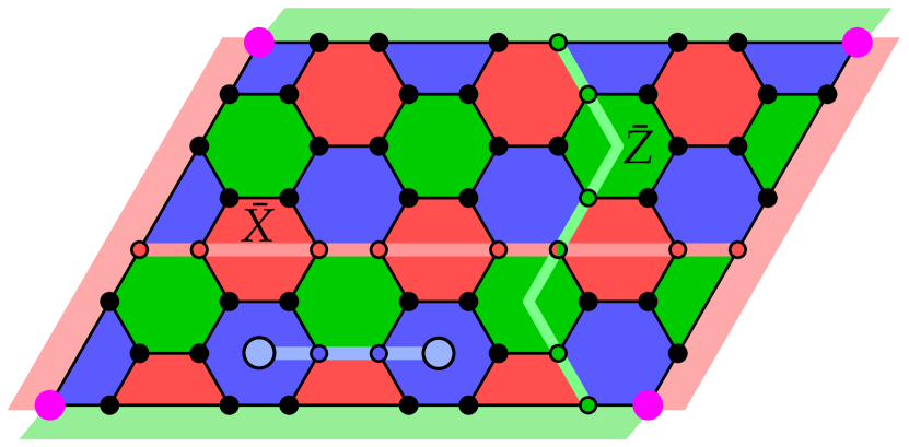
Figure 1: MSC patch encoding a single logical qubit. Plaquettes are colored red, green or blue. An example of a blue bond operator is highlighted. This operator creates two anyons (blue dots) on the blue plaquettes at its endpoints. The boundaries of the patch are red or green as shown; they are assigned the colors not featured in boundary plaquettes. Logical operators $\bar{X}$ and $\bar{Z}$ correspond to red and green string operators respectively, which terminate on same-colored, opposite boundaries. The termination of such strings signals the absorption of anyons at the boundaries; the boundary colors thus match the color of anyon species (red, green or blue) they can “condense”. Twist defects or, equivalently, corners between boundaries of different types are indicated by pink dots.

We define the MSC on a trivalent, three-colorable lattice [MjFerm_Surface_Code] (i.e., a lattice whose plaquettes can each be assigned one of three colors, such that no two adjacent plaquettes have the same color). In general, the plane has several trivalent, three-colorable tilings [Bombin_Color_Codes]. Among these, we focus on the honeycomb lattice, a patch of which is shown in Figure 1. Majorana operators $\gamma_{i}$ are assigned to sites of the lattice. Plaquettes are assigned one of three colors, red, green or blue, as shown in Figure 1. Each plaquette $p$ has an associated plaquette operator $\mathcal{O}_{p}=i^{|\partial p|/2}\prod_{j\in\partial p}\gamma_{j}$, where $\partial p$ is $p$’s boundary and where we choose an arbitrary (but definite) ordering of the product. The stabilizer group $\mathcal{S}$ is then generated by the complete set of $\mathcal{O}_{p}$ in the system. In Figure 1, there are $n=30$ Majoranas and $m=29$ independent stabilizer generators. Hence there is $k=1$ logical qubit encoded in the patch.

Bonds are also assigned a color, namely that of the plaquettes at their ends. A bond operator associated with bond $e$, connecting Majoranas $\gamma_{j}$ and $\gamma_{k}$, is defined as $\mathcal{O}_{e}=i\gamma_{j}\gamma_{k}$. A string $S$ is a set of bonds that all have the same color. String operators are then given by the product of all associated bond operators: $\mathcal{O}_{S}=\prod_{e\in S}\mathcal{O}_{e}$. Logical operators of the MSC are string operators that commute with all plaquette operators. For the patch in Figure 1, these correspond to strings running between opposite boundaries. In general, boundary conditions determine the number of logical qubits in the code. The patch in Figure 1 contains one logical qubit, which has logical operators given by the string operators $\bar{X}$ and $\bar{Z}$ shown. To see that $\bar{X}$ and $\bar{Z}$ anticommute note that their strings intersect an odd number of times; this renders $|A\cap B|$ odd in Equation (2). As noted earlier, logical operators can be deformed by stabilizers ($L\mapsto Ls$ for $s\in\mathcal{S}$) while still acting in the same manner on logical qubits. In the MSC, these deformations map between different string operators running between the same boundaries. Thus, in Figure 1, the equivalence class $[\bar{X}]$ contains all string operators terminating on horizontally opposite boundaries and similarly, $[\bar{Z}]$ contains all string operators terminating on vertically opposite boundaries.

II.4 Anyons in the MSC

Anyons are quasi-particle excitations of two-dimensional, topologically ordered systems [Anyon_Stats_Wilczek1984, Wen_FQH_GS_Degen, Bravyi_Kitaev_Codes_with_Bdry, Kitaev_Anyons2006, Non-Abelian_TQC_Review]. In topological quantum codes, we can define a stabilizer Hamiltonian according to which errors in the code correspond to anyons [Kitaev_toric_code, Kitaev_Anyons2006]. The MSC, owing to its fermionic nature, has an anyon content that differs significantly from bosonic codes [MjFerm_Surface_Code]. We review the MSC’s anyon model here.

One can assign a stabilizer Hamiltonian to the MSC by $H=-\frac{u}{2}\sum_{p}\mathcal{O}_{p}$, where $u>0$ and the sum runs over all plaquettes in the lattice. Thus the ground states of the Hamiltonian are code states of the MSC. Excited states are created by applying string operators to one of the ground states $\ket{\psi}$. If string operator $\mathcal{O}_{S}$ anti-commutes with plaquette operators $\mathcal{O}_{p_{1}},\ldots,\mathcal{O}_{p_{k}}$, then $\mathcal{O}_{S}\ket{\psi}$ has energy $ku$ above the ground state energy. We interpret plaquettes $p_{1},\ldots,p_{k}$ as hosting anyons and $\mathcal{O}_{S}$ as creating these anyons (or annihilating anyons already located at those sites, if $\mathcal{O}_{S}$ acts on an excited state). An anyon is labelled with the same color as the plaquette that hosts it: $\mathsf{R}$, $\mathsf{G}$ or $\mathsf{B}$ for those hosted on red, green or blue plaquettes respectively. The simplest string operator is a bond operator; this creates a pair of anyons at its endpoints, such as those indicated by blue dots in Figure 1. If we consider two blue bonds $e_{1}$ and $e_{2}$ that have endpoint plaquettes $p,q$ and $q,r$ respectively, applying $\mathcal{O}_{e_{1}}$ to $\ket{\psi}$ is interpreted as creating anyons on $p$ and $q$. Then subsequently applying $\mathcal{O}_{e_{2}}$ is interpreted as annihilating the anyon on $q$ and creating one on $r$. Alternatively, it can be thought of as moving the anyon from $q$ to $r$. Thus applying string operators to an excited state can move the anyons to any other plaquette of the same color as the anyon.

There also exist parity-non-conserving processes that create anyons in triplets, rather than pairs. For example, applying a Majorana operator $\gamma_{j}$ to a ground state creates three anyons located on the plaquettes surrounding $\gamma_{j}$. Due to the 3-colorability of the lattice, these anyons will all be colored differently.

Along with the three anyons mentioned, we also interpret the vacuum (no anyons present) as a quasi-particle, labelled $\mathbf{1}$. This will allow us to formalize fusion: the process of bringing two anyons close together and viewing the result as a separate anyon. For example, the fusion of $\mathsf{R}$ and $\mathsf{B}$ can be viewed as the anyon $\mathsf{BR}$. A triplet of anyons created by a single Majorana operator is also considered as a distinct anyon, $\mathsf{RGB}$. Note that creating a single $\mathsf{RGB}$ from $\mathbf{1}$ is not a fermion parity conserving process. To highlight this, we break the anyon content of the model into two sets, $\{\mathbf{1},\mathsf{R},\mathsf{G},\mathsf{RG}\}$ and $\{\mathsf{RGB},\mathsf{GB},\mathsf{BR},\mathsf{B}\}$ [MjFerm_Surface_Code], where the second set is obtained from the first by fusion with $\mathsf{RGB}$. We have the following (commutative and associative) fusion rules, dictating how anyons can be combined or split:

$$\mathbf{1}\times\mathsf{A}=\mathsf{A},\;\mathsf{A}\times\mathsf{A}=\mathbf{1}\quad(\text{for all anyons }\mathsf{A})$$

$$\mathsf{A}\times\mathsf{C}=\mathsf{AC}\quad(\text{for all anyons }\mathsf{A}\neq\mathsf{C}).$$ (3)

The fusion rules imply that anyons can be created (via splitting from an initial set) only in color-neutral combinations. All anyons in the system must be able to annihilate back to the initial set of anyons. There are two initial sets, $\mathbf{1}$ and $\mathsf{RGB}$, which are inequivalent because $\mathsf{RGB}$ cannot transform to $\mathbf{1}$ under any fermion parity conserving process. These anyons and fusion rules thus describe a system with a $\mathbb{Z}_{2}$ fermion parity grading [MjFerm_Surface_Code]. We discuss the braiding statistics of these anyons in Appendix LABEL:app:Anyon_Statistics.

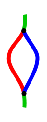
(a)

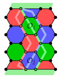
(b)

Figure 2: An example of string operator fusion. (a) Schematic illustration of a green string splitting into blue and red strings away from its endpoints. Black dots indicate single Majorana operators, at which points strings of three colors fuse. (b) A lattice-based illustration of the same phenomenon. The blue and red strings arise from the green string via multiplication by stabilizers $\mathcal{O}_{1}$ and $\mathcal{O}_{2}$.

Similarly to anyons, string operators also obey fusion rules. Viewing $\mathsf{C}$ as the endpoint of string operator of color $\mathsf{C}\in\{\mathsf{R},\mathsf{G},\mathsf{B}\}$ and $\mathbf{1}$ as the identity operator, we can apply Equations (II.4) to string operators even away from their endpoints. (We equate $\mathsf{RGB}$ with $\mathbf{1}$ in this context because an $\mathsf{RGB}$ pair can be created by a Majorana pair without string operators.) Fusion and splitting of string operators is implemented by multiplication with stabilizers. For example, the green string operator $\bar{Z}$ in Figure 1 can be split, by multiplication with green stabilizers, into blue and red strings (i.e. products of blue and red bond operators) along its length. This is shown in Figure 2. Hence the non-trivial rules from Equations (II.4) for string operators become $\mathsf{R}=\mathsf{G}\times\mathsf{B}$ and all cyclic permutations of this.

II.5 Boundaries in the MSC

Topological systems sometimes admit gapped boundaries, with a classification that is possible purely by considering the model’s anyon content (see Appendix LABEL:app:Lagrangian_subgroups for details). A system is gapped if the gap in energy between ground and lowest-energy excited states is bounded from below by a constant independent of the system size. Gapped boundaries of topological models are not only important from a condensed matter perspective [Kitaev_Kong, Protected_Edge_Modes], but also play an important role in quantum computation [Bravyi_Kitaev_Codes_with_Bdry, BBrown_Twists_CC, QC_with_Gapped_Boundaries2017].

In the MSC there exist three topologically-distinct types of gapped boundary, which can be colored red, green and blue respectively. They are distinguished from one another by the color of string operator that can terminate on that boundary. (Equivalently by the plaquette color not appearing on the boundary.) For example, in Figure 1, the top and bottom boundaries are green, since the green string operator $\bar{Z}$ terminates on both of them. Equivalently, any green anyons present in the system may be brought into proximity of a green boundary, where local, fermion-parity-preserving processes (e.g. the application of a green bond operator) can result in the anyon being absorbed by the boundary: we say that the anyon “condenses” at that boundary. $\mathsf{C}$-boundaries (for $\mathsf{C}=\mathsf{R},\mathsf{G},\mathsf{B}$) can condense only $\mathsf{C}$-anyons. Beyond this classification, fermionic systems have an extra $Z_{2}$ fermion parity grading along their one-dimensional boundaries. We will explore this further in the next section.

III Twist Defects of the Majorana Surface Code

If $\varphi$ is a permutation of the anyon labels, we say that $\varphi$ is a symmetry if it preserves the fusion rules and statistics (see Appendix LABEL:app:Anyon_Statistics) of the anyons [Barkeshli_defects_gauging2019]. In two-dimensional topologically ordered systems, (transparent) domain walls are one-dimensional defects that are associated with symmetries of the anyon labels [Kitaev_Kong, Twist_Symmetry_Review_Teo_2016, Barkeshli_defects_gauging2019]. An anyon $a$ crossing the wall (in a given direction) is transformed into $\varphi(a)$ where $\varphi$ is the symmetry associated with the domain wall. If $a$ crosses the wall in the opposite direction, it is transformed into $\varphi^{-1}(a)$.

Domain walls can terminate at point-like twist defects (“twists” for short) [Kitaev_Kong, Twist_Symmetry_Review_Teo_2016, Barkeshli_defects_gauging2019, Wen_Twists2013, Barkeshli_Nematic_States2012, Defects_Abelian_states, Twists_genons, Twist_Liquid]. It has been shown that these twist defects are closely related to non-Abelian anyons [Bombin_Twists, TEE_with_twist, Defects_Abelian_states, Dua_Twists_Majorana_stats], and can be used for topological quantum computation in surface codes [Holes_Twists_SurfaceCode, Bombin_Twists, Bombin_twists_code_deformation, Twists_genons, Webster_Bartlett_Defects2020]. Twists can be classified by the permutation that is enacted on an anyon encircling the twist in a clockwise direction. If a domain wall associated with symmetry permutation $\varphi$ terminates at two twists, one will be a $\varphi$ twist, and the other will be a $\varphi^{-1}$ twist.

We now introduce the twist defects appearing in the MSC. While some examples of MSC twists have previously appeared in the literature [Maj_Ferm_Codes, QC_with_MFCs], we establish here their fundamental features and provide their exhaustive categorization [Twist_note]. In this model we have three non-vacuum anyon labels (either $\{\textsf{R},\textsf{G},\textsf{B}\}$ or $\{\textsf{RG},\textsf{GB},\textsf{BR}\}$) that can be permuted in any way while still preserving the anyonic data, and hence the anyons possess an $S_{3}$ symmetry. Any non-identity element of the permutation group $S_{3}$ either swaps a pair of labels, generating a cyclic group $Z_{2}$, or it is a length-3 cycle, generating the subgroup $Z_{3}$. Thus domain walls and twists in the MSC are either of type $Z_{2}$ or $Z_{3}$.

Beyond this classification, we can further identify sub-types. There are three types of $Z_{2}$ twists, which we label $T_{\textsf{R}}$, $T_{\textsf{B}}$ and $T_{\textsf{G}}$, according to the color of the anyon that is preserved when wound completely around the twist. There are two types of $Z_{3}$ twists, labelled $T_{\mathsf{RGB}}$ and $T_{\mathsf{RGB}}^{-1}$. The former enacts the cycle $\mathsf{R}\rightarrow\mathsf{G}\rightarrow\mathsf{B}\rightarrow\mathsf{R}$ on anyons wound clockwise around the twist, and the latter enacts the inverse cycle. We provide lattice-based realizations of $Z_{2}$ and $Z_{3}$ twists in Figure 3. Discussion of these sub-types is convenient, but note that we can inter-convert twists between sub-types by relabelling the plaquettes. Indeed, a relabeling of an area $A$ of code in this way amounts to having introduced a closed loop of domain wall at its boundary $\partial A$. Similarly, by relabeling an area adjacent to the domain wall, we can, effectively, move the path of the wall. This shows that domain walls – but not the locations of their endpoints – are gauge dependent. Furthermore, if the loop of domain wall encircles a twist, it can change a $Z_{2}$ twist’s sub-type to any other within the $Z_{2}$ class ($T_{\mathsf{B}}$, $T_{\mathsf{G}}$ or $T_{\mathsf{R}}$) and, similarly, can map between the two $Z_{3}$ twist sub-types ($T_{\mathsf{RGB}}$ and $T_{\mathsf{RGB}}^{-1}$). See Appendix LABEL:app:Gauge_Dependence for further details of such gauge dependencies.

             

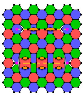
(a)

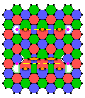
(b)

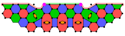
(c)

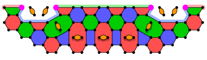
(d)

Figure 3: Lattice realizations of twists and logical MZMs in the MSC. In (a) and (b), twists and domain walls are indicated by pink dots and yellow dashed lines respectively. The Majoranas around the boundary of floating orange, pill-shape faces belong to the original honeycomb lattice but, after the introduction of twists, are not included in any plaquette operators. We introduce additional stabilizers, represented by the orange faces, to remove the degeneracy from these Majorana operators. In (a) we display an example of bosonic $Z_{2}$ twists, specifically of type $T_{\mathsf{B}}$ (top), and of $Z_{3}$ twists (bottom) and the domain walls connecting them. In (b) we display the fermionic counterparts of each of these twists and the resulting change to the orange stabilizers. In (c), a fermionic stretch of boundary is displayed, with pink dots indicating corners. Unpaired MZMs exist at the ends of the green boundary. Local changes to the stabilizer group result in the lattice in (d), which expands the unpaired MZMs into logical MZMs hosted on the odd-length blue boundaries.

Twists in the MSC differ from those in bosonic models in an important way: they can be further subdivided into “bosonic” and “fermionic” types of twist. These differ by a single MZM. However, rather than an extra MZM simply furnishing the twists, as might be expected, in Figure 3 we show that in fact the result can be a logical MZM located at the twist (cf. Section II.1). In Figure 3a we provide a lattice realization of bosonic $Z_{2}$ and $Z_{3}$ twists and the domain walls connecting them, while in Figure 3b we show $Z_{2}$ and $Z_{3}$ fermionic twists. In the latter, the lattice contains pentagonal holes. The (Hermitian) product of all Majorana operators around the boundary of this hole is a fermion-parity-odd operator that, by Equation (2), commutes with all plaquette operators. These operators cannot be included in the stabilizer group, owing to their odd fermion parity. Instead they are logical MZMs. They generalize the key features of MZMs, including their commutation with the Hamiltonian. We discuss these logical MZMs appearing at fermionic twists below, in Section III.3.

A domain wall lying along a boundary can change the color of that boundary, since it alters the color of anyons condensing there. Thus, there is an association between twists and corners, or interfaces between boundaries of different types (see Appendix LABEL:app:Twists_Corners) [BBrown_Twists_CC]. In Figure 1, we have indicated the corners between R and $\mathsf{G}$ boundaries in the MSC using pink dots. When such corners are fermionic, they host an MZM (see Figure  3c).

Twists can also be fused or split. For example, a $Z_{3}$ twist can be split into two $Z_{2}$ twists of different sub-types; this follows from $S_{3}$ being generated by transpositions (i.e., $Z_{2}$ operations) [rotman2000first]. However, the splitting or fusion of twists must preserve their overall fermionic or bosonic character: it cannot change the number of logical MZMs (mod 2). When a fermionic corner is split, logical MZMs appear, associated with boundaries of odd-length (see Figure  3d). Appendix LABEL:app:Twists_fusion has further twist fusion details and examples.

When the MSC is defined on the honeycomb lattice, some Majoranas along domain walls are not included in any plaquettes. In Figure 3a and 3b, we draw orange, pill-shape faces between pairs of Majoranas left out of the lattice in this way. These Majorana operators furnish extraneous fermion modes (cf. Section II.1), so we introduce additional bilinear stabilizers ($i\gamma_{a}\gamma_{b}$, for left-out operators $\gamma_{a}$, $\gamma_{b}$), represented by the orange faces in Figure 3, to remove the ground-state degeneracy associated with these modes, i.e., to remove these states from our code space. Those Majorana operators included in orange stabilizers are not included in any other stabilizer of the code. These extraneous Majorana operators, along with the logical MZMs at the twists, form a system similar to the Kitaev chain [Kitaev_chain2001]: a one-dimensional string of adjacent, nearest-neighbor Majorana bilinears. Considering this chain, we can also show how a transition between fermionic and bosonic twists can take place: it requires the chain to go through a topological phase transition. This corresponds to a change of the chain Hamiltonian (i.e., domain wall stabilizer set) along its entire length, so that the bilinears change from one assignment of adjacent nearest neighbors to the other. These two sets can be seen in Figures 3a and 3b. The transition results in the appearance or disappearance of “unpaired” logical MZMs (analogous to the unpaired MZMs at the ends of a regular Kitaev chain) at the twist defects. The existence of these two types of twists thus corresponds to the existence of a topologically non-trivial phase for one-dimensional fermionic systems, as modeled by the Kitaev chain [Turner_Fermion_Phases_1D2011, Kitaev_Fermion_Phases_1D2011, Defects_Abelian_states]. The fermionic or bosonic nature of a twist is as robust as this topological phase; it is immutable under local, fermion-parity-conserving processes.

III.1 Quantum Dimensions of Twists

The ground state degeneracy of a code with twist defects (or equivalently the dimension of the code space) is governed by the quantum dimension of those twists. Given a code with $N$ twists of quantum dimension $d$, the dimension of the code’s ground space grows as $d^{N}$ for large $N$. The quantum dimensions of twists in the MSC differ between bosonic and fermionic types, due to fermionic twists also contributing to the degeneracy via their logical MZMs.

We can calculate these quantum dimensions by counting the number of anyons that can “localize” at a given twist. An anyon is localized at a twist if it is brought close to that twist and absorbed through local processes. For example, if anyon $a$ obeys $a=b\times c$ and twist $\varphi$ is such that $\varphi(b)=\bar{c}$ (the anti-particle of $c$, such that $c\times\bar{c}=\mathbf{1}$), then anyon $a$ can be dragged to the vicinity of a twist, then split into anyons $b$ and $c$. $b$ is then wound clockwise around the twist and thus transformed to $\bar{c}$ which can then annihilate with $c$. This process results in anyon $a$ being localized at the twist. The quantum dimension of a twist $d_{\varphi}$ is given by $d_{\varphi}^{2}=\sum_{a\in\mathcal{A}}N_{a,\varphi}$, where $\mathcal{A}$ is the collection of anyons the system permits, and $N_{a,\varphi}$ is $1$ if anyon $a$ can be localized at $\varphi$, and $0$ otherwise [BBrown_Twists_CC].

Let us now count the anyons that can localize at each type of twist. Some of these localization processes are shown in Figure 4. Trivially, all twists localize the vacuum particle $\mathbf{1}$. Additionally, for bosonic $Z_{2}$ twists, anyon $\mathsf{RG}$ can localize at $T_{\mathsf{B}}$, $\mathsf{GB}$ at $T_{\mathsf{R}}$ and $\mathsf{BR}$ at $T_{\mathsf{G}}$. We do not count $\mathsf{B}$ as localizing at $T_{\mathsf{B}}$, nor similarly for the other twists, because in order to split $\mathsf{B}$ to $\mathsf{R}\times\mathsf{G}$, we need to introduce an $\mathsf{RGB}$ anyon to the system, and hence the twist is localizing $\mathsf{RGB}\times\mathsf{B}=\mathsf{RG}$, rather than just the $\mathsf{B}$ anyon. However we can localize $\mathsf{B}$ at a fermionic $T_{\mathsf{B}}$ twist, because a blue string operator can directly terminate at the odd-length, blue boundary associated with this twist (see Figure 3b), and thereby commute with all stabilizer generators in the vicinity of the twist. Fermionic twists also localize $\mathsf{RGB}$ anyons since, for example, $\mathsf{RGB}=\mathsf{B}\times\mathsf{RG}$, so one can split $\mathsf{RGB}$ into these two anyons. Then both $\mathsf{B}$ and $\mathsf{RG}$ can localize at $T_{\mathsf{B}}$. Thus bosonic $Z_{2}$ twists localize two types of anyons (including $\mathbf{1}$), while fermionic $Z_{2}$ twists localize four.

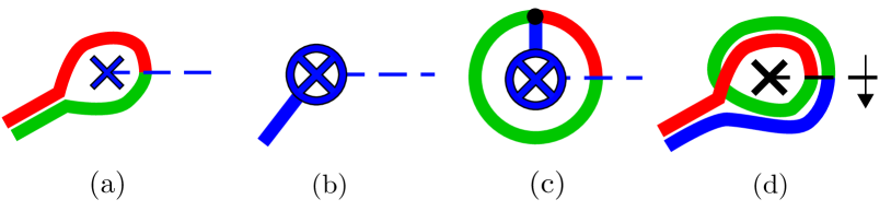
Figure 4: Schematic illustration of examples of anyon localization. Bosonic twists are indicated by crosses, and fermionic twists by circles containing crosses. Domain walls are indicated by dashed lines. Solid blue/red/green lines are string operators. (a) $\mathsf{RG}$ anyon localized at a bosonic $T_{\mathsf{B}}$ twist indicated in blue. (b) $\mathsf{B}$ anyon localized at a fermionic $T_{\mathsf{B}}$ twist indicated in blue. (c) $\mathsf{RGB}$ particle localized at a fermionic $T_{\mathsf{B}}$ twist. String operators of three different colors meet at a single Majorana operator (black dot). (d) $\mathsf{BR}$ anyon is localized at a bosonic $T_{\mathsf{RGB}}$ twist indicated in black. The arrow on the domain wall indicates the direction in which an anyon crossing the wall undergoes the permutation $T_{\mathsf{RGB}}$.

Bosonic $Z_{3}$ twists can localize $\mathsf{RG}$, $\mathsf{GB}$ and $\mathsf{BR}$ (and $\mathbf{1}$), since these particles can be split into their constituents (e.g. $\mathsf{BR}=\mathsf{B}\times\mathsf{R}$), one of which can be wound either once or twice around the twist until it is transformed into the same type as its partner (e.g. $\mathsf{R}$ transformed into $\mathsf{B}$, as shown in Figure 4). Fermionic $Z_{3}$ twists also have an odd-length boundary of a single color and hence can localize either $\mathsf{R}$, $\mathsf{G}$ or $\mathsf{B}$ in the same manner as fermionic $Z_{2}$ twists. However, $\mathsf{R}$, $\mathsf{G}$ and $\mathsf{B}$ can be transformed into one another by encircling the twist, and hence fermionic $Z_{3}$ twists can localize all three of these. Finally, they also localize $\mathsf{RGB}$, similarly to fermionic $Z_{2}$ twists. Thus in total, fermionic $Z_{3}$ twists can localize all eight anyons.

From the above, we can see that bosonic $Z_{2}$ twists have quantum dimension $d_{2}^{B}=\sqrt{2}$. This signals their similarity to Ising anyons [Bombin_Twists]. Fermionic $Z_{2}$ twists have quantum dimension $d_{2}^{F}=2$. Bosonic $Z_{3}$ twists have quantum dimension $d_{3}^{B}=2$, whereas fermionic $Z_{3}$ twists localize all anyons and hence have quantum dimension $d_{3}^{F}=2\sqrt{2}$. These quantum dimensions are verified using a different method in Appendix LABEL:app:Quantum_Dimensions.

MZMs are also similar to Ising anyons [MZM_TQC_Review2015]; hence they also have quantum dimension $\sqrt{2}$. This precisely equals the ratio between fermionic and bosonic twist quantum dimensions. Thus going from bosonic to fermionic twists can be seen as attaching an MZM, or a logical MZM, to the defect, as discussed previously.

III.2 Logical Qubits from Twists

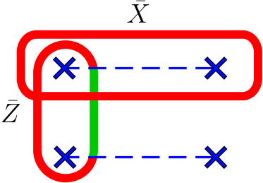
(a)

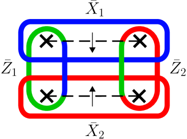
(b)

Figure 5: Schematic illustration of logical operators for examples of $Z_{2}$ (a) and $Z_{3}$ (b) twist defects (either bosonic or fermionic; we depict bosonic twists here). Twists are shown as crosses, domain walls as dashed lines, and string operators as solid lines, colored according to their type. The $Z_{2}$ twists and domain walls shown are of type $T_{\mathsf{B}}$. For the $Z_{3}$ twists and domain walls, the arrows indicate the direction in which a particle crossing the wall undergoes the permutation $T_{\mathsf{RGB}}$.

The degeneracy associated with twist defects discussed in the preceding section can be exploited for quantum computation. Introducing $k$ pairs of bosonic $Z_{2}$ twists of a single type (e.g. $T_{\mathsf{B}}$) into the MSC, results in $2^{k-1}$ additional ground states and hence $k-1$ additional logical qubits. (The $-1$ is because it takes at least four twists to get a set of logical operators. This is analogous to at least four Ising anyons being needed to furnish a qubit [Non-Abelian_TQC_Review].) For reasons discussed below, we will refer to this type of logical qubit as a “bosonic twist (BT) qubit” and the information it stores as “bosonic logical information.”

Logical operators for these BT qubits correspond to string operators encircling pairs of twists. Specifically, if $l$ is a set of red bonds forming a closed loop around a pair of $T_{\mathsf{B}}$ twists, then the red string loop $\prod_{(j,k)\in l}i\gamma_{j}\gamma_{k}$ is a logical operator. The fact that it is not in the stabilizer group results from the inability to deform it past any of the twists. If one could do this, it would change the number of $\mathsf{RG}$ anyons localized at that twist, and hence violate the total color conservation of anyons in the system. The conjugate logical operator is given by a red/green string operator encircling a pair of twists and crossing two domain walls (see Figure 5a). Blue string operators encircling $T_{\mathsf{B}}$ twists are stabilizer operators.

We schematically illustrate the logical operators associated with four $Z_{2}$ twists in Figure 5a, using colored lines to indicate string operators. The operators $\bar{X}$ and $\bar{Z}$ shown anti-commute, since different-colored string operators that cross each another once intersect at a vertex, and hence anti-commute. These logical operators generate the full algebra of operators acting on the logical qubit created by the addition of four twists to the system.

In Figure 5b we illustrate the logical operators for four $Z_{3}$ twists. In the figure, an anyon crossing a domain wall in the direction of the arrows is transformed according to the permutation $T_{\mathsf{RGB}}$, while those crossing in the opposite direction are transformed according to the inverse permutation. As can be seen, four $Z_{3}$ twists permit twice the number of logical operators as four $Z_{2}$ twists, owing to the extra degeneracy they afford (cf. Section III.1).

There is an arbitrariness to the logical operators shown. In Figure 5a, one may wrap blue string operators around the two upper-most or left-most twists (these operators are stabilizer elements). The blue strings can be fused with the logical operators indicated, in the sense outlined in Section II.4, thereby changing the red string operators to green ones and vice versa. If the code is embedded on a sphere, red and green string operators encircling all four twists are stabilizers, since they may be deformed around to the other side of the sphere, where they are not encircling any twists. With different boundary conditions, this becomes complicated, and we deal with these cases in the following section. For now, we continue with the simple case of a sphere. Operators $\bar{X}$ and $\bar{Z}$ can then be deformed into operators that instead circle the bottom two and two right-most twists respectively. In Figure 5b, one cannot change the colors of the strings, since any string operator encircling a pair of $Z_{3}$ twists is not a stabilizer. But on a sphere, all strings may be deformed to encircle the other two twists in the set of four.

Twists can admit either sparse or dense encodings of logical qubits. This is analogous to encodings with MZMs [MZM_TQC_Review2015]. In a dense encoding, $2k+2$ twists encode $k$ logical qubits. In sparse encodings, certain logical operators from the dense encoding become stabilizers, thereby lowering the number of logical qubits. For example, in a collection of $4k$ $T_{\mathsf{B}}$ twists, we can promote to stabilizers all red (and hence also green) string operators surrounding each group of four twists. This results in $k$ logical qubits, each stored within one group of four twists, and having the logical operators shown in Figure 5a.

III.3 Logical MZMs from Fermionic Twists

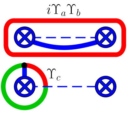
(a)

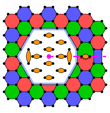
(b)

Figure 6: Logical MZMs in the MSC with fermionic twists (blue circles containing crosses). In (a) a logical MZM $\Upsilon_{c}$ and a logical MZM bilinear $i\Upsilon_{a}\Upsilon_{b}$ are represented as string operators, the latter being the product of the red string encircling the two twists, and the blue string terminating on the twists. The holes associated with fermionic twists may be enlarged, so long as the resulting boundary has odd length. An example is shown in (b), with the location of the twist and domain wall indicated by a pink dot and dashed line respectively.

Both bosonic and fermionic twists in the MSC host the BT qubits discussed above. This same type of topological degeneracy is seen in twists of qubit-based codes, which is why we refer to it as “bosonic.” For fermionic twists in the MSC we will label the corresponding bosonic logical operators as $\bar{X}_{B}$ and $\bar{Z}_{B}$. In addition, fermionic twists also host logical MZMs. In the same way as four physical MZMs can store a single qubit in a fermionic parity sector [MZM_TQC_Review2015], so too can four logical MZMs $\Upsilon_{a},\Upsilon_{b},\Upsilon_{c},\Upsilon_{d}$. We can also define encoded Pauli operators acting on the qubits stored by these logical MZMs. For example, for four logical MZMs, we may have “fermionic” logical operators $\bar{X}_{F}=i\Upsilon_{a}\Upsilon_{b}$ and $\bar{Z}_{F}=i\Upsilon_{a}\Upsilon_{c}$. We will refer to qubits stored in this way as “fermionic twist (FT) qubits.” Figure 6a shows the operator $i\Upsilon_{a}\Upsilon_{b}$ for two twists, deformed such that it is the product of a red string operator encircling the twists, and a blue string operator terminating on the two twists. It also shows the representation in terms of string operators of a single logical Majorana $\Upsilon_{c}$, which is equivalent to the localization of an $\mathsf{RGB}$ anyon at that twist (cf. Section III.1).

The logical operators $\bar{X}_{F}$ and $\bar{Z}_{F}$ have low minimum weights but large diameters, if the twists are far-separated (cf. Section II.1). If only fermion parity conserving (FPC, i.e., even-weight) errors can occur, FT qubits are protected by the twists’ separation [Maj_Ferm_Codes]. (Here we assume local coupling to the environment so that elementary FPC error operators are locally supported; all possible FPC error operators are products of these elementary FPC operators.) In realistic setups, however, we also have to contend with quasi-particle poisoning (QPP) resulting in non-FPC errors. The simplest such error operator is a single Majorana operator. To protect FT qubits from QPP, we can grow the size of the odd-length boundaries associated with twists and hence grow the weights of logical MZMs. As such (assuming we also increase twist separation), the FT qubits will have larger distances and so an increased protection against QPP noise. An example of such an enlarged hole is shown in Figure 6b.

Note that in systems where FPC errors are more common than QPP events, and if the former have below-threshold error rates, we can reduce the logical error rate to a low value set by QPP by increasing only the twist separation (i.e., increasing the code diameter but not the distance). This contrasts to MSC strategies without logical MZMs, where the code distance must be increased to reduce the logical error rate. Using fermionic twists in systems with low QPP probability, we can store double the number of logical qubits with only a minor increase in overheads, resulting from the size of the odd-boundary holes (see Figure 6b). While for low enough QPP probability microscopic MZMs could be used to store topological qubits, without error-correcting codes such a strategy is not fault-tolerant as any finite QPP rate will inevitably limit the coherence times of the topological qubit. Meanwhile, using logical MZMs, logical error rates resulting from QPP can be made arbitrarily small by increasing the code distance, provided the QPP rate is below the corresponding error threshold.

Logical MZMs can also appear in systems with only bosonic twists, when a boundary is introduced to the system. To our knowledge, this type of logical MZM has not been identified previously in the literature. We introduce it in Appendix LABEL:app:Logical_Maj_Boundary.

IV Fault-Tolerant Computation With Twists

In this section we detail how to perform fault-tolerant quantum computation with FT and BT qubits. These procedures will require the ability to move twists via “code deformation” (Section IV.1). In Section IV.2 we discuss how to prepare logical Pauli eigenstates and apply Clifford gates to BT qubits. In Sections IV.3 and IV.5 we discuss performing measurements of BT and FT logical operators. The above, combined with the preparation of magic states (Section IV.4), is sufficient for universal computation with both types of qubit.

IV.1 Code Deformation

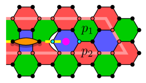
(a)

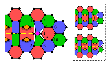
(b)

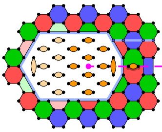
(c)

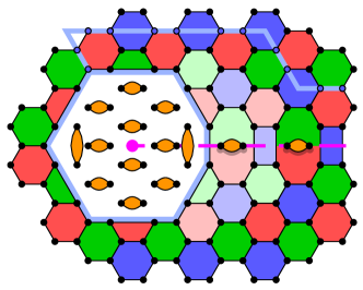
(d)

Figure 7: Code deformation to move bosonic (a)-(b) and fermionic (c)-(d) twists (pink dots). Domain walls are yellow/pink dashed lines. (a) A $Z_{2}$ bosonic twist along with part of a logical operator (red string), deformed away from the twist. To move the twist one plaquette to the right, we measure the bilinear with the light blue Majorana operators and merge the stabilizers at plaquettes $p_{1,2}$. (b) A $Z_{3}$ bosonic twist. After measuring the new stabilizers $\gamma_{1}\gamma_{2}\gamma_{3}\gamma_{4}$ and $\gamma_{3}\gamma_{4}\gamma_{5}\gamma_{6}$, the stabilizer generators appear as shown in the top inset. Performing two more bilinear measurements produces the stabilizers shown in the bottom inset. The result of these measurements is that the twist is moved to the right. (c) The hole from Figure 6b, associated with a fermionic twist, is enlarged to the left by measuring all light-colored operators. The blue string operator indicated commutes with all these measurements. (d) The hole is shrunk from the right by measuring all light-colored operators. The same blue string operator is now deformed to meet the hole on the left-hand side, where it commutes with all of these measurements.

For fault-tolerant computation using twists, we need to understand how to move them. We can do this with code deformation [Bombin_twists_code_deformation, Bombin_Code_Deformation, Punctures_Raussendorf_2006, Raussendorf_2007, Gauge_Color_Code]: a process where a code with stabilizer group $\mathcal{S}$ is mapped to another code with stabilizer group $\mathcal{S}^{\prime}$. To project to a code state of $\mathcal{S}^{\prime}$, we perform measurements of its stabilizer generators. In particular, in the new code those previous $\mathcal{S}$ stabilizer elements that anti-commute with any $s^{\prime}\in\mathcal{S}^{\prime}$ are replaced. While this changes the code’s stabilizer group, it preserves the logical state if each logical operator equivalence class $[L]$ of the original code has members that are also logical operators of the new code.

Here we introduce a novel code deformation procedure for the MSC that allows us to move twists. The procedure differs between fermionic and bosonic twists.

IV.1.1 Moving Bosonic Twists

The code deformation procedure for bosonic $Z_{2}$ twists is illustrated in Figure 7a. In the figure, a $T_{\mathsf{B}}$ twist along with part of a logical operator (a red string operator encircling this and another twist) are shown. To move the twist to the blue plaquette to its right, we measure the bilinear $\upsilon$ involving Majorana operators at the two light-blue sites. This then becomes an orange stabilizer along the newly enlarged domain wall. Since $\upsilon$ anticommutes with the plaquette operators $\mathcal{O}_{p_{1}}$ and $\mathcal{O}_{p_{2}}$ (indicated in the figure), these two operators are not included in $\mathcal{S}^{\prime}$. However their product $\mathcal{O}_{p_{1}}\mathcal{O}_{p_{2}}$ commutes with $\upsilon$ and hence is included as an 8-body stabilizer element. Note that measuring $\upsilon$ means that the blue hexagonal plaquette formerly hosting the twist can be replaced by a rectangular (4-body) plaquette: the new stabilizer generator is the product of $\upsilon$ and the original hexagonal plaquette operator.

The logical operator in the figure commutes with the updated stabilizer group. In general, we can always deform these string-like logical operators away from twists [bravyi2009no, Maj_Ferm_Codes], so that they commute with the code deformation measurements performed. Thus, twists can be moved via series of small steps like the above, without destroying the information stored in logical qubits.

In Figure 7b, a $Z_{3}$ bosonic twist is illustrated. If we again wish to move this twist to the right, we first measure the rectangular operators $\gamma_{1}\gamma_{2}\gamma_{3}\gamma_{4}$ and $\gamma_{3}\gamma_{4}\gamma_{5}\gamma_{6}$, with the vertex numbering indicated in the figure. Again, these operators anti-commute with certain members of the original stabilizer group $\mathcal{S}$. After measuring both rectangular operators, the adjacent red, green and blue hexagonal operators to their right are replaced by a 10-body operator (see upper inset of Figure 7b). The rectangular operators both commute with the operator defined on the twist’s original location, $\mathcal{O}_{T}=i\gamma_{1}\gamma_{2}\gamma_{5}\gamma_{6}\gamma_{7}\gamma_{9}$. The product of the two rectangular operators is $-\gamma_{1}\gamma_{2}\gamma_{5}\gamma_{6}$ and multiplying this with $\mathcal{O}_{T}$, we find that the bilinear $i\gamma_{9}\gamma_{7}$ is a stabilizer element. This is shown in orange in the top inset of Figure 7b. We then measure operators $i\gamma_{7}\gamma_{8}$ and $i\gamma_{9}\gamma_{10}$. This produces the same orange operators as in other locations along the domain wall. By following how the stabilizer group is updated after each of these two measurements, we see that they result in the stabilizer generators indicated in the lower inset of Figure 7b.

We can similarly move twists in different directions or generate a pair of twists in the lattice by measuring the stabilizer generators of the new code lattice. If any of these measurements return a $-1$ result, we can simply define the new stabilizer generators to be the negative of all measured operators whose eigenvalues are $-1$.

Moving the twists a short distance (compared to the twist separation) does not change the encoded states of the BT qubits, since the changes are restricted to be far from the paths of a suitable set of logical operators. However we shall see that performing a large sequence of small code deformation steps can result in unitary transformations of the code states.

IV.1.2 Moving Fermionic Twists

This procedure must preserve the information stored both by BT qubits and by logical MZMs. As above, the former can be ensured by deforming bosonic logical operators away from the twists. However, logical MZMs cannot be deformed in such a way: their support always has an odd-weight intersecton with the boundary associated with the twist (cf. Figure 6a).

Code deformation can most easily be seen to preserve information in MZMs by considering moving an enlarged hole, such as the one in Figure 6b. We move this hole through a series of enlarging and contracting procedures. In Figure 7c, the hole from Figure 6b is enlarged to the left by measuring the bilinear operators indicated in light-orange in Figure 7c, along with the four-body plaquette operators colored light-green and light-red in the figure. Figure 7d then shows the same hole shrunk from the right by measuring the light-colored plaquette operators indicated. The final result is that the location of the hole, and hence the twist, has moved to the left.

To see the preservation of the logical state, consider the logical operators in Figure 6a. The logical operator $i\Upsilon_{a}\Upsilon_{b}$ is the product of a string operator encircling twists $a$ and $b$, and a string operator connecting twists $a$ and $b$. Similarly, any parity-even product of logical MZMs can be deformed into an operator that intersects each of the twists’ boundaries at a single site (e.g. operator $i\Upsilon_{a}\Upsilon_{b}$ in Figure 6a). Other sections of the fermionic logical operator can be deformed away from the twists during code deformation, but the string operator(s) terminating on the twist boundaries cannot. The procedure will preserve fermionic information if we can deform these operators so that their support intersects none of the sites involved in the measurements to be performed. In Figure 7c we indicate such a string operator terminating on the right-hand side of the boundary of a $T_{\mathsf{B}}$ twist - this is unaffected by the measurements that enlarge the hole. In Figure 7d we indicate the same string operator, deformed to terminate on the left-hand side of the boundary. This operator is now unaffected by the measurements that shrink the hole. Hence the information stored in these logical MZMs is protected during code deformation.

IV.2 State Preparation of BT qubits and Clifford Gates via Braiding Twists

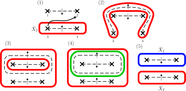
Figure 8: A braid of $Z_{3}$ twist $T_{3}$ around the pair $T_{1}$ and $T_{2}$ results in an entangling gate between the logical qubits. We show how this braid affects the logical operator $\bar{X}_{2}$. In panel (3) we have altered the location of the domain wall between $T_{3}$ and $T_{4}$ with a relabeling of plaquettes (see Appendix LABEL:app:Gauge_Dependence). In panel (5) we have deleted the closed loop of domain wall with another relabeling.

We will now discuss how to prepare logical Pauli eigenstates and perform fault-tolerant Clifford gates using BT qubits. The latter will be achieved purely by braiding $Z_{2}$ and $Z_{3}$ twists, in analogy to Clifford gate procedures in the bosonic Color Code [Bombin_twists_code_deformation] (though Clifford gates may also be achieved through lattice surgery; see Section IV.5). Our MSC scheme requires no ancilla logical qubits for the implementation of single-qubit Clifford gates, unlike other approaches [MjFerm_Surface_Code, Roadmap_to_MSCs]. We shall consider BT qubits stored sparsely in quartets of either $Z_{2}$ (storing one qubit in four twists) or $Z_{3}$ (two qubits in four twists) bosonic twists. We will see that we need only consider two sub-types of $Z_{2}$ twist, which we take (without loss of generality) to be $T_{\mathsf{B}}$ and $T_{\mathsf{R}}$.

To prepare four $Z_{2}$ twists in an eigenstate of a given logical Pauli operator, we start with a MSC patch hosting these twists, such as the one of Figure 1. For example, to prepare this patch in the $+1$ eigenstate of $\bar{X}$ (a red string operator), we initialize the patch in the $+1$ eigenstate of all red bond operators. This prepares $\bar{X}$ and green and blue plaquette operators in their $+1$ eigenstates since they are all products of red bond operators. To prepare red plaquette operators in their $+1$ eigenstates, we measure them and apply red string operators that take the state to the code space given the observed syndrome (in practice, we would not apply this operator and instead, redefine the stabilizers). Since $\bar{X}$ and the green/blue plaquette operators commute with the red plaquette operators, these measurements do not change their eigenvalues from the preceding step. The inequivalent choices of string in the last step differ by $\bar{X}$; this is again immaterial given we already had a $+1$ eigenstate of $\bar{X}$. This procedure thus prepares the patch in the $+1$ eigenstate of $\bar{X}$ in the code space. We can then move the twists away from the boundaries of the patch using code deformation (cf. Section IV.1). Finally, we can fuse the patch with the rest of the lattice hosting logical information by adding stabilizer operators that bridge the gap between the boundaries of the two lattices.

As is possible in the bosonic surface code [Holes_Twists_SurfaceCode], we can braid bosonic twists in the MSC to perform certain encoded Clifford gates on logical qubits. This procedure is achieved with code deformation via sequences of small steps. It is a naturally fault-tolerant procedure, since the code distance (and the diameters of logical operators) can be kept large throughout the whole braiding process. If we were restricted to using $Z_{2}$ twists of a single type (e.g. $T_{\mathsf{B}}$) then, just as in the bosonic surface code, braiding could not generate the entire Clifford group for the logical qubits. Braiding $T_{\mathsf{B}}$ twists can generate only the single-qubit Clifford gates, as explained in Appendix LABEL:app:Braiding. This is due to the similarity between bosonic $T_{\mathsf{B}}$ twists and Ising anyons [Non-Abelian_TQC_Review], as is also the case in the surface code [Bombin_Twists, TEE_with_twist].

However, unlike the bosonic surface code, the MSC also has $Z_{3}$ twist defects and hence allows for a larger set of gates to be implemented by braids. This is similar to the case of the bosonic Color Code [Bombin_twists_code_deformation]. We can enact an entangling gate between the two qubits stored in a quartet of $Z_{3}$ twists by using the braid shown in Figure 8. If we call this braiding operation $B$, it can be seen from the figure that the operator $\bar{X}_{2}$ is mapped to $B\bar{X}_{2}B^{\dagger}=\bar{X}_{1}\bar{X}_{2}$ by this braid. Similarly (see Appendix LABEL:app:Braiding), the other logical Pauli operators are transformed as: $\bar{X}_{1}\rightarrow\bar{X}_{2}$, $\bar{Z}_{1}\rightarrow\bar{Y}_{1}\bar{Y}_{2}$ and $\bar{Z}_{2}\rightarrow\bar{Z}_{1}\bar{X}_{2}$. We can fix the signs in these mappings by carefully defining the logical operators and stabilizer generators. It can be verified that $B$ is equivalent to the following circuit between the two logical qubits:

$$\Qcircuit@C=1em@R=1.5em{\lstick{1}&\gate{S}\gate{H}\gate{S}\ctrl{1}\gate{S}\gate{H}\gate{S}\targ\qw\\ \lstick{2}\qw\gate{X}\qw\targ\gate{S}\gate{H}\gate{S}\ctrl{-1}\qw}$$

A $Z_{3}$ twist can be split into two differently-colored $Z_{2}$ twists (cf. Appendix LABEL:app:Twists_fusion). Splitting all four $Z_{3}$ twists into $T_{\mathsf{B}}$ and $T_{\mathsf{R}}$ twists results in qubit 1 being stored between the $T_{\mathsf{R}}$ twists and qubit 2 between the $T_{\mathsf{B}}$ twists. Thus, through this splitting, we can enact all single-qubit Clifford gates on qubits $1$ and $2$ with $Z_{2}$ twist braids. We can therefore achieve the full set of Clifford gates on qubits 1 and 2 via twist braids (note that a CNOT gate controlled on qubit 1 and targeted on qubit 2 can be achieved with the gate $\bar{Z}_{1}\bar{H}_{1}B^{3}\bar{H}_{1}$, where $\bar{H}_{1}$ is the Hadamard gate acting on qubit 1).

To enact a Clifford circuit on $n$ BT qubits, we can store some of them in $T_{\mathsf{B}}$ twists and the rest in $T_{\mathsf{R}}$ twists. This allows single-qubit Cliffords to be implemented within same-color quartets and entangling gates to be implemented between $T_{\mathsf{B}}$-stored and $T_{\mathsf{R}}$-stored qubits with the above procedures. We can also entangle $T_{\mathsf{B}}$-stored (equivalently $T_{\mathsf{R}}$-stored) qubits by introducing a quartet of $T_{\mathsf{G}}$ twists as an ancilla qubit. Entangling gates between the ancilla and the two logical qubits (which are possible due to the above discussion) are all that is required to perform an entangling gate on the two logical qubits.

IV.3 State Preparation of FT qubits and Logical Majorana Parity Measurements via Lattice Surgery

To compute with the logical MZMs of fermionic twists, we need the ability to prepare eigenstates, perform computational basis measurements, and perform logical $B_{4}$ and $T_{2}$ gates, which have the form $B_{4,abcd}=\exp(i\frac{\pi}{4}\Upsilon_{a}\Upsilon_{b}\Upsilon_{c}\Upsilon_{d})$ and $T_{2,ab}=\exp(\frac{\pi}{8}\Upsilon_{a}\Upsilon_{b})$ respectively. In general we may also wish to perform $B_{2k}=\exp{(i^{k+1}\frac{\pi}{4}\Upsilon_{j_{1}}\ldots\Upsilon_{j_{2k}})}$ gates as these too are fermionic variants of Clifford gates acting on FT qubits. While these could be synthesised from $B_{4}$ gates [FPBC], it may be preferable to perform them directly. We also want to perform all of these fermionic gates while preserving the bosonic information stored in the twists. We will, similarly to the previous section, detail how to achieve this with $T_{\mathsf{B}}$ and $T_{\mathsf{R}}$ twists as this will be sufficient for universal computation.

We can perform $B_{2k}$ gates if we can prepare ancilla logical MZMs furnishing known eigenstates and measure arbitrary logical MZM products, i.e., logical fermion parity operators [Bravyi_Kitaev_Fermionic_QC2002]. The ability to perform these measurements also allows us to prepare eigenstates of operators $i\Upsilon_{a}\Upsilon_{b}$ for arbitrary logical MZMs $a,b$. In this section, we detail how to prepare patches of code that host ancilla logical MZMs, and how to perform logical fermion parity measurements. In the next section, we detail how to perform $T_{2}$ gates. This, combined with the above, allows us to perform universal computation with logical MZMs.

IV.3.1 Bilinear Measurement and Eigenstate Preparation

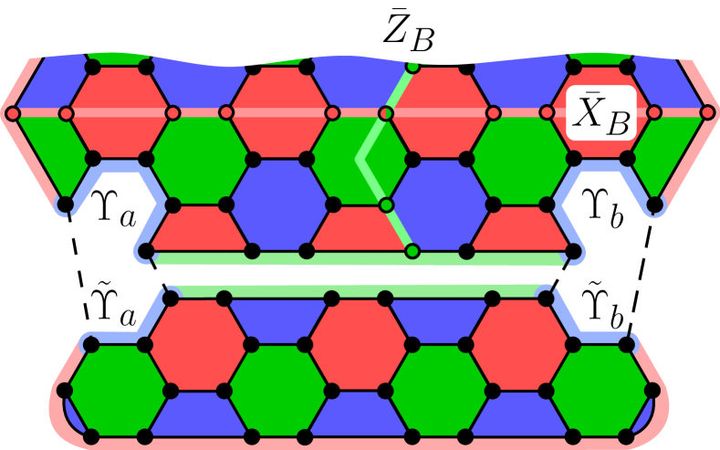
Figure 9: Fault-tolerant measurement of $i\Upsilon_{a}\Upsilon_{b}$ through lattice surgery with a neighbouring MSC patch containing ancillary logical MZMs $\tilde{\Upsilon}_{a}$ and $\tilde{\Upsilon}_{b}$. A small MSC section is shown in the top part of the figure. This patch contains the logical MZMs to be measured ($\Upsilon_{a}$ and $\Upsilon_{b}$), and some BT qubits. Some examples of bosonic logical operators ($\bar{X}_{B}$ and $\bar{Z}_{B}$) are shown. The ancilla MSC patch, shown in the bottom of the figure, is prepared in the $+1$ eigenstate of $i\tilde{\Upsilon}_{a}\tilde{\Upsilon}_{b}$. Operators $\tilde{\Upsilon}_{a}$ and $\tilde{\Upsilon}_{b}$ are associated with the length-$3$ blue boundary sections. $i\Upsilon_{a}\tilde{\Upsilon}_{a}$ and $i\Upsilon_{b}\tilde{\Upsilon}_{b}$ are eight-body plaquette operators indicated by dashed lines. The measurement of these two operators fuses the two patches together along their blue boundary sections.

The simplest measurement to consider is that of logical MZM bilinears, i.e. operators of the form $i\Upsilon_{a}\Upsilon_{b}$. This type of measurement may appear at the end of a fermionic circuit (sampling the output distribution) and can also be used to prepare computational basis states for the start of a circuit. To perform such a measurement in a non-destructive, fault-tolerant manner, we first prepare an ancillary pair of logical MZMs ($\tilde{\Upsilon}_{a}$ and $\tilde{\Upsilon}_{b}$) in a separate patch of code located close to the first. This ancilla patch is shown in Figure 9. Note that this patch contains no BT qubits, owing to its boundary conditions. Comparing this patch with the one in Figure 1, we see that while in the latter, there exist multiple inequivalent logical operators running between separated boundaries of the same color ($\bar{X}$ and $\bar{Z}$ in Figure 1), the ancilla patch in this case has only one such string operator, a blue string terminating on the two blue boundary sections. This is equivalent to the operator $i\tilde{\Upsilon}_{a}\tilde{\Upsilon}_{b}$. The patch can be prepared in the $+1$ eigenstate of $i\tilde{\Upsilon}_{a}\tilde{\Upsilon}_{b}$ by, similarly to the preparation of BT qubits, preparing the $+1$ eigenstate of all blue bond operators, then measuring all blue stabilizers, and applying a correction string if needed.

To measure $i\Upsilon_{a}\Upsilon_{b}$ on the neighbouring patch of code, we merge the twists supporting $\Upsilon_{a}$ and $\Upsilon_{b}$ with a boundary colored differently from the twists, so that the logical Majoranas are located along the exterior boundary of the lattice (see Figure 3d and 9). For $T_{\mathsf{B}}$ and $T_{\mathsf{R}}$ twists we merge the twists with a green-colored boundary. In Figure 9 we show an example in which $\Upsilon_{a}$ and $\Upsilon_{b}$ are both supported along blue boundaries. See Appendix E for a more general example.

We can measure operators $i\Upsilon_{a}\tilde{\Upsilon}_{a}$ and $i\Upsilon_{b}\tilde{\Upsilon}_{b}$ by fusing the blue boundaries associated with the logical Majoranas, thus forming an extra blue plaquette operator (see Figure 9). We begin by measuring the operator $i\Upsilon_{a}\tilde{\Upsilon}_{a}$, obtaining the result $\eta_{a}$. This operator anticommutes with both $i\Upsilon_{a}\Upsilon_{b}$ and $i\tilde{\Upsilon}_{a}\tilde{\Upsilon}_{b}$, but the effect of the measurement is simply to logical-braid $\Upsilon_{a}$ with $\tilde{\Upsilon}_{b}$ [Bravyi_PBC2016, FPBC]. To see this, note that if the pre-measurement state is $\ket{\psi}$ [which by construction satisfies $(i\tilde{\Upsilon}_{a}\tilde{\Upsilon}_{b})\ket{\psi}=\ket{\psi}$], then the post-measurement state is $\frac{1}{\sqrt{2}}[1+\eta_{a}(i\Upsilon_{a}\tilde{\Upsilon}_{a})]\ket{\psi}$ which equals

$$B_{2,ba}\ket{\psi}=\frac{1}{\sqrt{2}}\left[1+\eta_{a}(i\Upsilon_{a}\tilde{\Upsilon}_{a})(i\tilde{\Upsilon}_{a}\tilde{\Upsilon}_{b})\right]\ket{\psi}$$ (4)

with the logical braid $B_{2,ba}=\exp(\eta_{a}\frac{\pi}{4}\tilde{\Upsilon}_{b}\Upsilon_{a})$.

$B_{2,ba}$ transforms logical Majoranas as: $B_{2,ba}\Upsilon_{a}B_{2,ba}^{\dagger}=\eta_{a}\tilde{\Upsilon}_{b}$ and $B_{2,ba}\tilde{\Upsilon}_{b}B_{2,ba}^{\dagger}=-\eta_{a}\Upsilon_{a}$. The operator we wish to measure, $i\Upsilon_{a}\Upsilon_{b}$, is thus mapped to $\eta_{a}i\tilde{\Upsilon}_{b}\Upsilon_{b}$ through the above measurement. Hence we must now measure the operator $i\tilde{\Upsilon}_{b}\Upsilon_{b}$, another blue plaquette operator fused from the corresponding blue boundaries. We denote the outcome by $\eta_{b}$. The desired measurement outcome of $i\Upsilon_{a}\Upsilon_{b}$ is thus $\eta_{a}\eta_{b}$. After these measurements, $-\eta_{a}\eta_{b}\Upsilon_{a}\Upsilon_{b}\tilde{\Upsilon}_{a}\tilde{\Upsilon}_{b}$ is a stabilizer of the resulting state of the full system. Finally, we measure $i\tilde{\Upsilon}_{a}\tilde{\Upsilon}_{b}$ destructively (i.e., via its constituents [Bravyi_Kitaev_Fermionic_QC2002]) to decouple the ancilla patch: we measure all blue bond operators of the patch, yielding the eigenvalue of $i\tilde{\Upsilon}_{a}\tilde{\Upsilon}_{b}\prod_{p\in B}\mathcal{O}_{p}$ with the blue stabilizers $\mathcal{O}_{p\in B}$ of the patch. We then measure these $\mathcal{O}_{p\in B}$ (or use previous syndrome measurement outcomes) and thereby infer the outcome $\tilde{\eta}_{ab}$ for $i\tilde{\Upsilon}_{a}\tilde{\Upsilon}_{b}$. This yields a $+1$ eigenstate of $\tilde{\eta}_{ab}\eta_{a}\eta_{b}i\Upsilon_{a}\Upsilon_{b}$. If $\tilde{\eta}_{ab}=-1$, this state is not the one corresponding to the obtained $i\Upsilon_{a}\Upsilon_{b}$ outcome $\eta_{a}\eta_{b}$. But this error can simply be classically tracked, and subsequent computations can be updated.

We can generalize this procedure to cases in which $\Upsilon_{a}$ and $\Upsilon_{b}$ have larger weights, and are hosted along boundaries of different colors. We outline the more involved setups required in Appendix E. In Section V, we compare the resource overheads for this method with other approaches and show that the use of ancilla logical MZMs generically results in a decrease in the Majorana overhead associated with measurement.

The bosonic information in the twists is again preserved by these lattice surgery procedures, since bosonic logical operators (such as $\bar{Z}_{B}$ and $\bar{X}_{B}$ of Figure 9) can be deformed away from all of the lattice surgery measurements.

We need not move twists to a distant boundary if they are deep within the code bulk. Instead, we can create a hole within the lattice by ceasing the stabilizer measurements within and altering the stabilizers along the boundary to ensure that it has a single color. We then introduce the MSC patch with the ancilla logical MZMs into this hole and proceed as above. Afterwards we fill in the hole by measuring the original plaquette operators. Such a hole may add an extra logical qubit, but if so, filling in the hole simply discards the qubit again. While the introduction of the hole will affect the weights of certain logical operators, and hence may reduce the code distance, this distance can still be kept arbitrarily large by increasing the separation of the code’s twists.

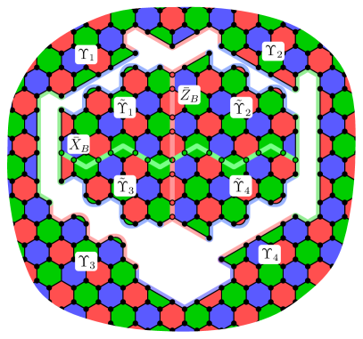
(a)

(b)

Figure 10: Lattice surgery procedure for measuring logical parity operator $-\Upsilon_{1}\Upsilon_{2}\Upsilon_{3}\Upsilon_{4}$. (a) Logical MZMs are supported on blue (for $\Upsilon_{1}$ and $\Upsilon_{2}$) or red (for $\Upsilon_{3}$ and $\Upsilon_{4}$) sections of odd-length boundaries on the patch surrounding the central hole. The patch inside the hole has ancilla logical MZMs ($\tilde{\Upsilon}_{1},\ldots,\tilde{\Upsilon}_{4}$) supported on blue, odd-length boundaries. It also encodes a BT qubit, with logical operators $\bar{X}_{B}$ (green string) and $\bar{Z}_{B}$ (red string) indicated. The lattice surgery involves measuring the plaquette operators connecting logical MZMs $\Upsilon_{j}$ and $\tilde{\Upsilon}_{j}$, for $j=1,2,3,4$. These plaquette operators are shown lightly colored in (b).

	Pre-measurement	$i\Upsilon_{1}\tilde{\Upsilon}_{1}$	$i\Upsilon_{2}\tilde{\Upsilon}_{2}$	$i\Upsilon_{3}\tilde{\Upsilon}_{3}$
Stabilizing Logical Operators	$\{\Gamma,\tilde{\Gamma}_{4},i\tilde{\Upsilon}_{1}\tilde{\Upsilon}_{2}\bar{X}_{B}$ $i\tilde{\Upsilon}_{2}\tilde{\Upsilon}_{4}\bar{Z}_{B}\}$	$\{\lambda_{1}i\Upsilon_{1}\tilde{\Upsilon}_{1},\Gamma\tilde{\Gamma}_{4},$ $i\tilde{\Upsilon}_{3}\tilde{\Upsilon}_{4}\bar{X}_{B},i\tilde{\Upsilon}_{2}\tilde{\Upsilon}_{4}\bar{Z}_{B}\}$	$\{\lambda_{1}i\Upsilon_{1}\tilde{\Upsilon}_{1},\lambda_{2}i\Upsilon_{2}\tilde{\Upsilon}_{2},$ $\Gamma\tilde{\Gamma}_{4},i\tilde{\Upsilon}_{3}\tilde{\Upsilon}_{4}\bar{X}_{B}\}$	$\{\lambda_{1}i\Upsilon_{1}\tilde{\Upsilon}_{1},\lambda_{2}i\Upsilon_{2}\tilde{\Upsilon}_{2},$ $\lambda_{3}i\Upsilon_{3}\tilde{\Upsilon}_{3},\Gamma\tilde{\Gamma}_{4}\}$
	$\Upsilon_{1}$	$i\lambda_{1}\tilde{\Upsilon}_{2}\tilde{\Upsilon}_{3}\tilde{\Upsilon}_{4}$	$-\lambda_{1}\tilde{\Upsilon}_{3}\bar{Z}_{B}$	$\lambda_{1}i\tilde{\Upsilon}_{4}\bar{X}_{B}\bar{Z}_{B}$
Logical MZMs	$\Upsilon_{2}$	$\Upsilon_{2}$	$\lambda_{2}\tilde{\Upsilon}_{4}\bar{Z}_{B}$	$\lambda_{2}\tilde{\Upsilon}_{4}\bar{Z}_{B}$
	$\Upsilon_{3}$	$\Upsilon_{3}$	$\Upsilon_{3}$	$\lambda_{3}\tilde{\Upsilon}_{4}\bar{X}_{B}$
	$\Upsilon_{4}$	$\Upsilon_{4}$	$\Upsilon_{4}$	$\Upsilon_{4}$
Measurement Operator	$\Gamma_{4}$	$-i\lambda_{1}\tilde{\Upsilon}_{2}\tilde{\Upsilon}_{3}\tilde{\Upsilon}_{4}\Upsilon_{2}\Upsilon_{3}\Upsilon_{4}$	$\lambda_{1}\lambda_{2}\tilde{\Upsilon}_{3}\tilde{\Upsilon}_{4}\Upsilon_{3}\Upsilon_{4}$	$i\lambda_{1}\lambda_{2}\lambda_{3}\Upsilon_{4}\tilde{\Upsilon}_{4}$

Table 1: Operators and their updates after each set of lattice surgery measurements. Top row: the operator measured by lattice surgery. First column: we track updates to the set of logical operators stabilizing the state, the logical MZMs $\Upsilon_{1},\ldots,\Upsilon_{4}$, and measurement operator $\Gamma_{4}$. The updates to these after measuring $i\Upsilon_{j}\tilde{\Upsilon}_{j}$ are shown in the respective columns. The final measurement $i\Upsilon_{4}\tilde{\Upsilon}_{4}$ is not considered, as this, unlike the preceding $i\Upsilon_{j}\tilde{\Upsilon}_{j}$, commutes with all stabilizing logical operators.

IV.3.2 Arbitrary Fermion Parity Measurement

We can measure arbitrary products $\Gamma_{2k}=i^{k}\prod_{j=1}^{2k}\Upsilon_{j}$ of logical MZMs similarly. We again treat the case in which all twists hosting the $\Upsilon_{j}$ are of types $T_{\mathsf{B}}$ or $T_{\mathsf{R}}$. We move the twists to a boundary of color different to all the twists (i.e., green), using code deformation. Similarly to above, this can either be an exterior boundary or we can introduce a hole in the center of the lattice. Now the logical MZMs are supported on $2k$ sections of odd-length boundary. A $k=2$ example where these boundary sections lie around a hole is shown in Figure 10.

An ancilla patch of code is then prepared close to the boundary that now hosts all $\Upsilon_{j}$. This patch will also host $2k$ logical MZMs labelled $\tilde{\Upsilon}_{j}$ for $j=1,\ldots,2k$, supported along the boundary of the patch. Each $\tilde{\Upsilon}_{j}$ is located close to $\Upsilon_{j}$ on the main lattice. The ancilla patch will have the $2k$-MZM parity operator $\tilde{\Gamma}_{2k}=i^{k}\prod_{j=1}^{2k}\tilde{\Upsilon}_{j}$. We choose these logical MZMs to be supported on blue sections of boundary. This patch will contain BT qubits as well as logical MZMs. Specifically, it encodes $k-1$ BT qubits. In Figure 10a we show the logical operators for the patch in the example considered.

We prepare the ancilla patch by first preparing all blue bonds within the patch in their $+1$ eigenstates and then measuring all blue plaquette operators. In the example of Figure 10, there are three independent logical operators for the ancilla patch that are made up only of blue string operators, as seen from representing logical MZM bilinears similarly to Figure 6a (but with the green $\bar{X}_{B}$ replacing the red loop of Figure 6a for $i\tilde{\Upsilon}_{1}\tilde{\Upsilon}_{2}$ and $i\tilde{\Upsilon}_{3}\tilde{\Upsilon}_{4}$): $i\tilde{\Upsilon}_{1}\tilde{\Upsilon}_{2}\,\bar{X}_{B}$, $i\tilde{\Upsilon}_{2}\tilde{\Upsilon}_{4}\,\bar{Z}_{B}$, and $-\tilde{\Upsilon}_{1}\tilde{\Upsilon}_{2}\tilde{\Upsilon}_{3}\tilde{\Upsilon}_{4}=\tilde{\Gamma}_{4}$. After preparation, the system will be in the $+1$ eigenstate of all three of these operators.

We now measure $i\Upsilon_{j}\tilde{\Upsilon}_{j}$, obtaining outcome $\lambda_{j}$, for all $j=1,\ldots,2k$, using lattice surgery. This involves measuring plaquette operators that bridge the gaps between logical MZMs $\Upsilon_{j}$ and $\tilde{\Upsilon}_{j}$. The product of these plaquette operators is equivalent to the operator $i\Upsilon_{j}\tilde{\Upsilon}_{j}$. Examples of these plaquette operators are shown in Figure 10b. Notice that, in this example, the product of blue plaquette operators connecting $\Upsilon_{1}$ and $\tilde{\Upsilon}_{1}$ give the outcome for $i\Upsilon_{1}\tilde{\Upsilon}_{1}$, since the green plaquette operators between these two boundaries are simply products of original four-body and two-body stabilizer generators. Similar situations apply to the measurement of $i\Upsilon_{2}\tilde{\Upsilon}_{2}$, $i\Upsilon_{3}\tilde{\Upsilon}_{3}$ and $i\Upsilon_{4}\tilde{\Upsilon}_{4}$.

To explain the effect of these $i\Upsilon_{j}\tilde{\Upsilon}_{j}$ measurements, we consider the example of Figure 10 more closely. Here we will use $\Gamma$ to denote the total fermion parity operator of the main lattice (containing $\Upsilon_{1},\ldots,\Upsilon_{4}$). Since $\Gamma$ is in the original stabilizer set, the system is initially in the $\Gamma=+1$ state. Before any lattice surgery measurements, there exist four independent logical operators that stabilize the full system (i.e. the system is in a $+1$ eigenstate of all these operators): $\Gamma$, $\tilde{\Gamma}_{4}$, $i\tilde{\Upsilon}_{1}\tilde{\Upsilon}_{2}\,\bar{X}_{B}$ and $i\tilde{\Upsilon}_{2}\tilde{\Upsilon}_{4}\,\bar{Z}_{B}$. The first measurement operator, $i\Upsilon_{1}\tilde{\Upsilon}_{1}$, anti-commutes with $\Gamma$, $\tilde{\Gamma}_{4}$ and $i\tilde{\Upsilon}_{1}\tilde{\Upsilon}_{2}\,\bar{X}_{B}$, and hence only products of pairs of these three operators continue to stabilize the state of the system. The full list of such (independent) stabilizing logical operators is: $\lambda_{1}i\Upsilon_{1}\tilde{\Upsilon}_{1}$, $\Gamma\tilde{\Gamma}_{4}$, $i\tilde{\Upsilon}_{2}\tilde{\Upsilon}_{4}\,\bar{Z}_{B}$ and $i\tilde{\Upsilon}_{1}\tilde{\Upsilon}_{2}\,\bar{X}_{B}\tilde{\Gamma}_{4}=i\tilde{\Upsilon}_{3}\tilde{\Upsilon}_{4}\,\bar{X}_{B}$. Similarly to Section IV.3.1, we may replace the projector associated with the logical measurement with a logical braid: $\exp(\frac{\pi}{4}\lambda_{1}i\Upsilon_{1}\tilde{\Upsilon}_{1}\tilde{\Gamma}_{4})=\exp(-\frac{\pi}{4}\lambda_{1}i\Upsilon_{1}\tilde{\Upsilon}_{2}\tilde{\Upsilon}_{3}\tilde{\Upsilon}_{4})$. This produces the correct post-measurement state. This operator can be thought of as a braid between $\Upsilon_{1}$ and $i\lambda_{1}\tilde{\Upsilon}_{2}\tilde{\Upsilon}_{3}\tilde{\Upsilon}_{4}$: it maps $\Upsilon_{1}\mapsto i\lambda_{1}\tilde{\Upsilon}_{2}\tilde{\Upsilon}_{3}\tilde{\Upsilon}_{4}$. Thus the operator $\Gamma_{4}$ we wish to measure is mapped to operator $-i\lambda_{1}\tilde{\Upsilon}_{2}\tilde{\Upsilon}_{3}\tilde{\Upsilon}_{4}\Upsilon_{2}\Upsilon_{3}\Upsilon_{4}$.

Further updates to the stabilizing logical operators, the logical MZMs $\Upsilon_{j}$, and to $\Gamma_{4}$ occur after $i\Upsilon_{2}\tilde{\Upsilon}_{2}$ and $i\Upsilon_{3}\tilde{\Upsilon}_{3}$ measurements. These updates can be found in Table 1. As can be seen in this table, after the measurement of $i\Upsilon_{3}\tilde{\Upsilon}_{3}$, $\Gamma_{4}$ is mapped to $i\lambda_{1}\lambda_{2}\lambda_{3}\Upsilon_{4}\tilde{\Upsilon}_{4}$. And so after the final measurement of $i\Upsilon_{4}\tilde{\Upsilon}_{4}$, with outcome $\lambda_{4}$, we learn the measurement outcome of $\Gamma_{4}$ to be $\lambda_{1}\lambda_{2}\lambda_{3}\lambda_{4}$, which is what we wanted to determine.

$\lambda_{1}\lambda_{2}\lambda_{3}\lambda_{4}$ is also the eigenvalue of the operator $\Gamma_{4}\tilde{\Gamma}_{4}=\prod_{j=1}^{4}i\Upsilon_{j}\tilde{\Upsilon}_{j}$. To disentangle ancilla and logical degrees of freedom, we measure all blue bond operators on the ancilla patch, from which we can infer the eigenvalues of $\tilde{\Gamma}_{4}$ (call it $\eta_{1}$), $i\tilde{\Upsilon}_{1}\tilde{\Upsilon}_{2}\,\bar{X}_{B}$ (call it $\eta_{2}$) and $i\tilde{\Upsilon}_{2}\tilde{\Upsilon}_{4}\,\bar{Z}_{B}$ (call it $\eta_{3}$). These operators do not commute with the operators $i\Upsilon_{j}\tilde{\Upsilon}_{j}$ but they do with $\Gamma_{4}\tilde{\Gamma}_{4}$. Hence from the previous measurement outcomes and the measured eigenvalue of $\tilde{\Gamma}_{4}$, we can find the $\Gamma_{4}$ eigenvalue to be $\eta_{1}\lambda_{1}\lambda_{2}\lambda_{3}\lambda_{4}$. If $\eta_{1}=-1$, we need to apply a correction to map the state to an eigenstate of $\Gamma_{4}$ with eigenvalue $\lambda_{1}\lambda_{2}\lambda_{3}\lambda_{4}$. This correction operation can simply be kept track of classically. There are multiple such possible correction operations owing to the degeneracy of the $\Gamma_{4}=\pm 1$ eigenspaces. To determine which we should apply, we need to determine if all logical bilinears ($i\Upsilon_{1}\Upsilon_{2}$, $i\Upsilon_{3}\Upsilon_{4}$, etc.) have been correctly preserved by the entire series of measurements above. We discuss the details of this in Appendix F.

Note that, similarly to the case of Section IV.3.1, this measurement procedure does not directly affect the bosonic information stored between the twists, as all bosonic logical operators can be deformed away from the locations of the lattice surgery measurements. The introduction of the hole again reduces the distance of some logical qubits, but this distance can be preserved by further separating the twists in the code. Hence all encoded information can remain topologically protected throughout the entire procedure.

IV.4 Magic State Injection

Combining the above operations with the injection of magic states into MSC patches allows one to perform universal quantum computation fault-tolerantly with both bosonic logical qubits and logical MZMs. Here we detail how to achieve magic state injection in two ways: the first is within an existing patch of code, while the second is in a separate patch of code (e.g., in an ancilla register).

Several noisy copies of this magic state can be purified to a single copy using Clifford gates and measurements [Magic_State_Dist]. “Magic state gadgets,” also composed of Clifford gates and measurements [nielsen_chuang], can be used to apply $T$ gates on BT or FT qubits in the code, using these purified magic states as a resource.

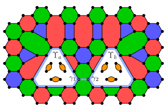
(a)

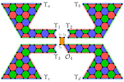
(b)

Figure 11: Code configurations for magic state injection. (a) On-patch injection. Two fermionic $T_{\mathsf{B}}$ twists are at minimal separation, with another two twists located far away (not shown). A magic state can be injected by preparing a suitable initial state and applying the gate $\exp(\frac{\pi}{8}\gamma_{1}\gamma_{2})$. Logical MZMs $\Upsilon_{a}$ and $\Upsilon_{b}$ reside on the blue boundaries shown. The blue bond operator $i\gamma_{1}\gamma_{2}$ is the logical $i\Upsilon_{a}\Upsilon_{b}\bar{Z}_{B}$, acting on both FT and BT qubits stored between the four twists. (b) Off-patch injection. Four MSC patches are prepared, each with two logical MZMs along blue boundaries (e.g. $\Upsilon_{a}$ and $\Upsilon_{1}$ indicated). A qubit with Majorana operators $\gamma_{1},\gamma_{2},\gamma_{3},\gamma_{4}$ (orange rectangle) is prepared in a magic state. Plaquette operators $\mathcal{O}_{j}=i\Upsilon_{j}\gamma_{j}$ (for $j=1,2,3,4$, with $\mathcal{O}_{4}$ shown) are measured to inject this magic state into the four-patch qubit furnished by $\Upsilon_{a}$, $\Upsilon_{b}$, $\Upsilon_{c}$, $\Upsilon_{d}$.

IV.4.1 On-Patch Magic State Injection

Figure 11a shows two fermionic twists (hosting logical MZMs $\Upsilon_{a}$, $\Upsilon_{b}$) at minimum separation. Suppose there exist another two twists at large separation from this pair (hosting logical MZMs $\Upsilon_{c}$, $\Upsilon_{d}$). For this setup, the logical operator $i\gamma_{1}\gamma_{2}$, shown in the figure, equals $i\Upsilon_{a}\Upsilon_{b}\bar{Z}_{B}$, where $\bar{Z}_{B}$ is a logical Pauli operator (green string loop encircling the two logical MZMs, not shown) for the BT qubit stored between the four twists. Hence, $i\gamma_{1}\gamma_{2}$ acts on both FT and BT qubits stored in the twist. To prepare a magic state, we first prepare the state $\ket{+}_{F}\ket{0}_{B}$ (cf. Sections IV.2 and IV.3.1), where $\ket{0}_{B}=\bar{Z}_{B}\ket{0}_{B}$ is a computational basis state of the BT qubit and $\ket{+}_{F}=i\Upsilon_{a}\Upsilon_{c}\ket{+}_{F}$ is a basis state of the FT qubit stored between $\Upsilon_{a},\Upsilon_{b},\Upsilon_{c},\Upsilon_{d}$. We then perform the rotation $\exp{(\frac{\pi}{8}\gamma_{1}\gamma_{2})}$; we assume we can perform at least a noisy version of this gate using established methods [Karzig_geom_magic_2016, Karzig_geom_magic_meas2019, Karzig_Majorana2017]. This approximately yields

$$\frac{1}{\sqrt{2}}\left(\ket{0}_{F}+e^{i\pi/4}\ket{1}_{F}\right)\ket{0}_{B}$$ (5)

where $\ket{0}_{F}$ and $\ket{1}_{F}$ are the $+1$ and $-1$ eigenstates of operator $i\Upsilon_{a}\Upsilon_{b}$, respectively.

Throughout this process, twists $a$ and $b$ are far-separated from twists $c$ and $d$, and hence $\bar{X}_{B}$ and $i\Upsilon_{a}\Upsilon_{c}$ logical errors are suppressed by this large separation, and the weights of the logical MZMs, which can be made arbitrarily large. So, provided error rates are below the error threshold, the BT qubit remains in the $\ket{0}_{B}$ state throughout the process with arbitrarily high probability, while the FT qubit is prepared in a noisy magic state. Alternatively, we could prepare the BT qubit in a magic state by instead first preparing the state $\ket{0}_{F}\ket{+}_{B}$. The same gate as above then approximately prepares the state:

$$\frac{1}{\sqrt{2}}\ket{0}_{F}\left(\ket{0}_{B}+e^{i\pi/4}\ket{1}_{B}\right).$$ (6)

We can also prepare magic states in both FT and BT qubits by enacting the following operators on the state $\ket{+}_{F}\ket{+}_{B}$:

$$\text{CX}_{F,B}\exp{\left(\frac{\pi}{8}\Upsilon_{a}\Upsilon_{b}\bar{Z}_{B}\right)}\text{CX}_{F,B}=\exp{\left(-i\frac{\pi}{8}\bar{Z}_{B}\right)},$$ (7)

$$\text{CX}_{B,F}\exp{\left(\frac{\pi}{8}\Upsilon_{a}\Upsilon_{b}\bar{Z}_{B}\right)}\text{CX}_{B,F}=\exp{\left(\frac{\pi}{8}\Upsilon_{a}\Upsilon_{b}\right)},$$ (8)

where $\text{CX}_{J,K}$ is the CNOT gate controlled on qubit $J$ and targeted on qubit $K$.

IV.4.2 Off-Patch Magic State Injection

In Figure 11b we illustrate injecting magic states into separate MSC patches via measurements. Four MSC patches are prepared, each with two logical MZMs. On each patch, one of these logical MZMs has low weight and the other has high weight. The low-weight logical MZMs are labelled $\Upsilon_{1}$, $\Upsilon_{2}$, $\Upsilon_{3}$, and $\Upsilon_{4}$ (cf. the weight-three logical MZMs in Figure 11b), and the large-weight logical MZMs are labelled $\Upsilon_{a}$, $\Upsilon_{b}$, $\Upsilon_{c}$, and $\Upsilon_{d}$, respectively (cf. the weight-seven logical MZMs of Figure 11b). These patches do not contain any BT qubits, owing to their boundary conditions. Our goal will be to inject a magic state into the four-patch FT qubit furnished by $\Upsilon_{a}$, $\Upsilon_{b}$, $\Upsilon_{c}$, and $\Upsilon_{d}$, i.e., using the large-weight MZMs.

We start by preparing the patches in the $+1$ eigenstates of $i\Upsilon_{a}\Upsilon_{1}$, $i\Upsilon_{b}\Upsilon_{2}$, $i\Upsilon_{c}\Upsilon_{3}$ and $i\Upsilon_{d}\Upsilon_{4}$ (cf. Section IV.3). We then prepare a patch with four Majorana operators (orange rectangle in Figure 11b and labelled $\gamma_{1},\gamma_{2},\gamma_{3},\gamma_{4}$) in a possibly noisy magic state encoded in subspace stabilized by the patch parity $-\gamma_{1}\gamma_{2}\gamma_{3}\gamma_{4}$. We inject this magic state into an FT qubit furnished by $\Upsilon_{a},\ldots,\Upsilon_{d}$ by measuring operators $\mathcal{O}_{j}=i\Upsilon_{j}\gamma_{j}$ for $j=1,2,3,4$. The example of $\mathcal{O}_{4}$ is represented as a plaquette operator in Figure 11b. This measurement maps $\gamma_{1}$ to $\Upsilon_{a}$ (and similarly for the other measurements), by the same logic that we have used repeatedly: due to the anticommutation of $\mathcal{O}_{1}$ and $i\Upsilon_{a}\Upsilon_{1}$, the measurement, with outcome $\lambda_{1}$ effectively implements the logical braid $\exp(\frac{\pi}{4}\lambda_{1}\Upsilon_{a}\gamma_{1})$. In this way, the magic state furnished by $\gamma_{1}$, $\gamma_{2}$, $\gamma_{3}$, $\gamma_{4}$ is transferred to the FT qubit furnished by logical MZMs $\Upsilon_{a},\Upsilon_{b},\Upsilon_{c},\Upsilon_{d}$ (specifically in the subspace stabilized by $-\Upsilon_{a}\Upsilon_{b}\Upsilon_{c}\Upsilon_{d}$), up to a correction operation (if $\lambda_{1}\lambda_{2}\lambda_{3}\lambda_{4}=-1$) which can be tracked. The resource cost of this magic state preparation method is compared with alternatives in Section V.

IV.5 Arbitrary String Operator Measurements

We now discuss measuring various string operators. The following considerations make this particularly interesting. The twist framework established above allows for not only fermionic and bosonic computation to be done side-by-side, but also for hybrid computing schemes involving both FT and BT qubits. To complete the set of universal gates for both types of logical qubit, we require a gate that entangles the two. This would, for example, allow us to use magic states stored in FT qubits (cf. Section IV.4) to apply $T$ gates to BT qubits. Moreover, the measurement of BT qubit logical operators opens up an additional route for implementing Clifford gates on top of braiding twists, which could result in reduced overheads [Lattice_surg_low_overhead].

We can achieve the effect of entangling gates between BT and FT qubits by fault-tolerantly measuring $\Gamma_{F}P_{B}$, where $\Gamma_{F}$ is a logical MZM parity and $P_{B}$ is a bosonic logical Pauli operator. For example, take an FT, a BT, and an ancilla twist qubit, with logical operators $\{\bar{Z}_{F},\bar{X}_{F}\}$, $\{\bar{Z}_{B},\bar{X}_{B}\}$ and $\{\bar{Z}_{A},\bar{X}_{A}\}$, respectively. To implement a CNOT gate controlled on qubit $F$ and targeted on $B$, we can measure $\bar{Z}_{F}\bar{Z}_{A}$, then $\bar{X}_{A}\bar{X}_{B}$ and then $\bar{Z}_{A}$. This results in the desired gate, up to a logical Pauli operator which can be tracked. We can avoid introducing these ancilla qubits by instead classically tracking Clifford gates and updating circuit measurements accordingly (see also Section V) [Bravyi_PBC2016, Tracking_Color_Codes, QC_with_MFCs].

Here, we detail how to measure arbitrary $\Gamma_{F}P_{B}$, all of which will be some product of string operators. We distinguish between two types of string operator, with arbitrary $\Gamma_{F}P_{B}$ operators being products of multiple instances of these two types. Define fermionic string operators as those that terminate on the odd-length boundaries associated with two fermionic twists, and bosonic string operators as simply products of bosonic logical operators (thus they are simply of the form $P_{B}$). The latter will either encircle some number of twists or alternatively terminate at a boundary of even length. Hence only fermionic string operators have a non-trivial action on FT qubits. We describe the measurement of fermionic string operators first, then move on to bosonic string operators. We describe how to measure arbitrary products of these two types in Appendix G.

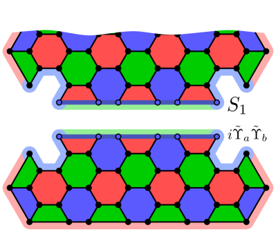
(a)

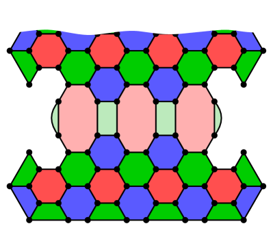
(b)

Figure 12: Lattice surgery procedure for measuring fermionic string operator $S_{1}$. The lower ancilla patch contains logical MZMs $\tilde{\Upsilon}_{a}$ and $\tilde{\Upsilon}_{b}$, while the upper patch contains logical information. (a) The setup before lattice surgery, with the ancilla patch prepared in the $i\tilde{\Upsilon}_{a}\tilde{\Upsilon}_{b}=+1$ state. Blue, red and green boundaries on both patches are indicated; blue boundaries host logical MZMs. Also indicated are blue string operators $S_{1}$ and $i\tilde{\Upsilon}_{a}\tilde{\Upsilon}_{b}$ running between blue boundaries on the logical and ancilla patches respectively. (b) Lattice surgery is performed, with extra operators fusing the two patches indicated with lightly colored plaquettes.

The procedures for measuring string operators use lattice surgery and are very similar to those for measuring fermion parity operators, as described in Section IV.3. We begin with the case of a single fermionic string operator, $S_{1}$. For concreteness, we assume that $S_{1}$ terminates on the boundaries of two (fermionic) $T_{\mathsf{B}}$ twists. As in Section IV.3.1, we move these two twists to a (green- or red-colored) boundary of the lattice, and introduce an ancilla patch of code nearby to this boundary, hosting two logical MZMs $\tilde{\Upsilon}_{a}$ and $\tilde{\Upsilon}_{b}$ (hosted on blue boundaries). Alternatively, a hole can be created in the lattice and the ancilla patch prepared in this hole, as described in previous sections. An example of the resulting setup is shown in Figure 12a. The ancilla patch is initialized in the $+1$ eigenstate of $i\tilde{\Upsilon}_{a}\tilde{\Upsilon}_{b}$ (cf. Section IV.3.1), which is a blue string operator. (The red string operator part of $i\tilde{\Upsilon}_{a}\tilde{\Upsilon}_{b}$, akin to that in Fig. 6a, would now connect the red boundaries and hence can be shrunk: it is a stabilizer element.)

To measure the operator $S_{1}$, we perform lattice surgery between the logical patch and the ancilla patch. For the example of Figure 12, we perform measurements of the green plaquette operators bridging the gap between the two patches. Notice that the product of these green plaquettes is equal to $\pm S_{1}(i\tilde{\Upsilon}_{a}\tilde{\Upsilon}_{b})$. This procedure differs from that of Section IV.3.1 since there we only measure two plaquette operators bridging the gap between the patches. Those plaquette operator measurements fused pairs of logical MZMs on the ancilla and code patches. In the present case we fuse the patches along the two string operators shown in Figure 12 resulting in different logical information being extracted. Call the product of all measurement outcomes of these green plaquette operators $\lambda$. Similarly to the cases examined in Section IV.3, $\lambda$ is the measurement outcome for $S_{1}$ that we desire (up to a known sign defined by the ordering of the operators). To decouple the ancilla patch, we then destructively measure $i\tilde{\Upsilon}_{a}\tilde{\Upsilon}_{b}$ (cf. Section IV.3.1). This produces the result $i\tilde{\Upsilon}_{a}\tilde{\Upsilon}_{b}$ with certainty (assuming perfect measurements) since we can find a representative of this logical operator that commutes with all lattice surgery measurements. Hence we need not track any correction operation, as we had to do in previously-described lattice surgery procedures.

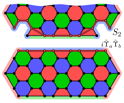
(a)

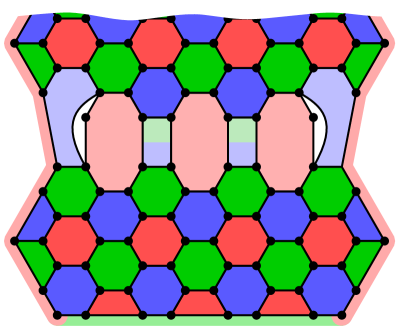
(b)

Figure 13: Lattice surgery procedure for measuring a bosonic string operator. Lattices before being fused are shown in (a): $S_{2}$ (red) is the bosonic string to be measured; the ancilla patch has logical MZMs $\tilde{\Upsilon}_{a}$ and $\tilde{\Upsilon}_{b}$ (red boundaries) with $i\tilde{\Upsilon}_{a}\tilde{\Upsilon}_{b}$ realized by the red string connecting them. The lattice after fusion is shown in (b), with the extra plaquettes connecting the two patches shown lightly colored.

We now explain the measurement of a bosonic string operator using lattice surgery. Without loss of generality we assume this is a red string operator, which we call $S_{2}$. If $S_{2}$ encircles some twists, we move these to one of the boundaries of the lattice, as before. Thus $S_{2}$ now terminates on even boundaries. An example involving two twists is shown in Figure 13a. The lattice hosting $S_{2}$ in this figure is the same as that hosting $S_{1}$ in Figure 12a. While the ancilla patch looks slightly different, it still only hosts two logical Majoranas $\tilde{\Upsilon}_{a}$ and $\tilde{\Upsilon}_{b}$. The patch is prepared in the $+1$ eigenstate of $i\tilde{\Upsilon}_{a}\tilde{\Upsilon}_{b}$, a red string operator shown in Figure 13a. Measuring the blue and green/blue plaquettes that fuse the two patches (shown lightly shaded in Figure 13b) measures the operator $S_{2}i\tilde{\Upsilon}_{a}\tilde{\Upsilon}_{b}$. These measurements commute with the fermionic logical operators on the upper patch and, moreover, do not reveal any information about them. Finally, the ancilla patch is destructively measured leaving the upper patch in the measured eigenstate of $S_{2}$.

In Appendix G, we extend these procedures to the measurement of arbitrary products of bosonic and fermionic string operators. Thus, any logical operator in the code can be measured using lattice surgery. We can therefore achieve universal quantum computation with BT and FT qubits side-by-side, by combining these measurements with the procedures of Sections IV.2-IV.4.

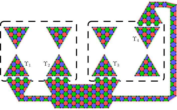
(a)

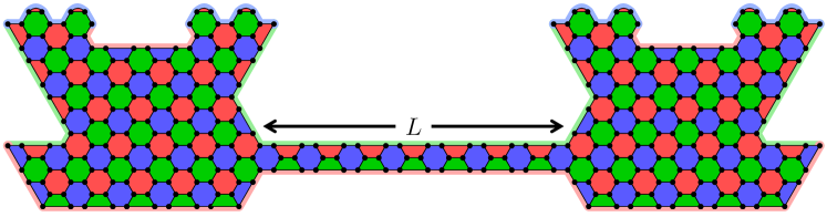
(b)

Figure 14: (a) Setup for measuring a two-qubit logical Pauli operator, with logical qubits encoded in Majorana triangle code quartets (in dashed boxes). The operator being measured is $\Upsilon_{1}\Upsilon_{2}\Upsilon_{3}\Upsilon_{4}$, with logical MZMs on triangle codes indicated. An ancilla patch hosts logical MZMs on blue boundaries. This patch is thin along the parts with red-green opposite boundaries, and $O(d)$ in the section with red-red opposite boundaries. (b) A $d=10$ ancilla patch used for long-range logical Pauli measurement. Blue boundaries host logical MZMs. The thin section runs between logical qubits and can be arbitrarily long.

V Overheads for Universal Fault-Tolerant Computation

	Qubit Storage	State Preparation	Single-Logical-Qubit Measurement	Long-range Measurement
All bosonic	$\frac{3}{2}d^{2}-2d+2$	$0$	$\frac{3}{2}d^{2}+O(d)$	$dL+O(d^{2})$
Fermionic qubits and bosonic ancillas	$\frac{3}{4}d^{2}+1$	$\geq\frac{3}{8}d^{2}-d+2$	N/A	N/A
All fermionic	$\frac{3}{4}d^{2}+1$	$O(1)$	$\frac{3}{8}d^{2}+O(d)$	$3L+O(d^{2})$

Table 2: Number of Majoranas required (as a function of code distance $d$) for Pauli-based computing with various schemes, utilizing either bosonic or fermionic aspects of the MSC. We compare the requirements for storing a logical qubit (1${}^{\text{st}}$ column), and the ancilla costs of preparing a magic state (2${}^{\text{nd}}$ column), measuring a single-qubit logical operator (3${}^{\text{rd}}$) and measuring a long-range multi-qubit logical Pauli operator (4${}^{\text{th}}$). 1${}^{\text{st}}$ row: Majorana requirements for storing magic states in BT qubits and using the same “bosonic” MSC patches (with no logical MZMs) for logical Pauli operator measurements [QC_with_MFCs]. For state preparation, only those MZMs in the storage patch are required and hence the ancilla cost is zero [QC_with_MFCs]. 2${}^{\text{nd}}$ row: requirements for storing qubits in Majorana triangle codes and using bosonic ancilla patches where possible [Maj_Triangle_Code2018]. 3${}^{\text{rd}}$ row: requirements for storing qubits in Majorana triangle codes and using ancilla patches that contain logical MZMs.

Universal quantum computation can be achieved via the measurement of arbitrary Pauli operators on (distilled) magic states [Bravyi_PBC2016, Mithuna_Magic_State_PBC2019]. Universal fermionic quantum computation, which is more suitable for fermionic simulation, can be performed in a similar manner [FPBC]. Here we demonstrate a resource-efficient method for preparing magic states in “Majorana triangle codes” [Maj_Triangle_Code2018] and performing Pauli measurements on these states. That is, we perform “Pauli-based computation” with the MSC, taking full advantage of the Gottesman-Knill theorem to reduce the quantum resources required. Our method is able to find avenues for increased resource savings by exploiting the fermionic aspects of the Majorana surface code that we have introduced above.

A Majorana triangle code is a patch of MSC encoding a single logical MZM. It has three odd-length boundaries of different colors (see Figure 14a). We begin by preparing $n$ magic states in $4n$ Majorana triangle codes, using for each quartet the method outlined in Section IV.4.2, followed by additional measurements to sever the “tails” in Figure 11b. (We assume having high-fidelity magic states, otherwise we can employ magic state distillation to improve the magic-state quality.) Let the distance of this encoding be $d$, meaning that the weights of the logical MZMs hosted on the four triangle codes are all $d/2$. We note that our state-injection procedure takes only a $d$-independent time (that of the measurements) to increase the distance of the logical qubit from $2$ to $d$. However, the code patches for magic state injection (cf. Figure 11b) include low-weight logical MZMs. These two features, respectively, act in favor and against the fidelity of the injected state.

In more detail, the four code patches prepared for the injection of a single magic state each contain two logical MZMs (i.e. $\Upsilon_{a}$ and $\Upsilon_{1}$, $\Upsilon_{b}$ and $\Upsilon_{2}$ etc. in Figure 11b). The patches look like a Majorana triangle code with a “tail,” terminating in the weight-three logical MZMs $\Upsilon_{j}$ ($j=1,2,3,4$). The lengths of these tails can be kept independent of the code distance. Increasing the tail length beyond a certain maximum length simply increases the diameter of operators $i\Upsilon_{a}\Upsilon_{1}$, $i\Upsilon_{b}\Upsilon_{2}$, etc., not the minimum weight $\frac{d}{2}+3$ of these operators. While this decreases the probability of parity-conserving processes resulting in logical errors such as $i\Upsilon_{a}\Upsilon_{1}$, these logical “errors” act as $+1$ on the initial state of the patch and hence are inoperative. Thus, the total number of constituent Majoranas involved in the preparation of a single (potentially noisy) magic state is $4\Delta_{d}+O(1)$, where $\Delta_{d}$ is the number of Majoranas in a single side-length-$d/2$ triangle code. After the magic states are prepared, the tails can be deleted, resulting simply in four triangle codes (see Figure 14a). For hexagonal, 6.6.6 codes (i.e. those with red, green and blue plaquettes having support on 6 Majoranas each) $\Delta_{d}=\frac{3}{16}d^{2}+\frac{1}{4}$ and for 4.8.8 codes (i.e. those with square and octagonal plaquettes [QC_with_MFCs]) $\Delta_{d}=\frac{1}{8}d^{2}+\frac{1}{2}(d-1)$. We will continue to analyse the resources of 6.6.6 codes, but we can obtain even lower overheads with 4.8.8 codes, at the cost of higher-weight stabilizer measurements.

In Table 2, we consider the Majorana overheads of storing a single magic state and the ancilla overhead of preparing this state. We compare our proposal with those that use fewer fermionic features of the MSC. Storing magic states in BT qubits has a larger overhead for an equivalent code distance [QC_with_MFCs] (i.e. storing a magic state in a patch like that of Figure 1). As can be seen from Table 2, storing a magic state in four triangle codes with a code distance of $d$ requires $4\Delta_{d}=\frac{3}{4}d^{2}+1$ Majoranas. But storing the same state in a distance-$d$ BT qubit requires $\frac{3}{2}d^{2}-2d+2$ Majoranas.

Previous work demonstrated computation with Majorana triangle codes but utilized only bosonic aspects of the MSC for the ancilla patches containing magic states [Maj_Triangle_Code2018]. This requires an $O(d^{2})$ number of ancilla Majoranas in addition to four triangle codes [Maj_Triangle_Code2018]. The ancilla cost is at least that of a distance-$d$ patch (e.g., that of Figure 1). This compares to the $O(1)$ number of ancilla Majoranas required in the above method. Thus, for large $d$, utilizing fermionic aspects of the MSC in magic state preparation and storage becomes much more efficient.

Using the fermionic features of the MSC also enhances the efficiency of logical qubit readout (cf. Section IV.3). We begin by considering the measurement of a single-qubit logical Pauli operator, which is of the form $i\Upsilon_{j}\Upsilon_{k}$, with $\Upsilon_{j}$ and $\Upsilon_{k}$ stored in separate Majorana triangle codes. We have outlined how to perform this type of measurement in Section IV.3.1 and Appendix E. The number of Majoranas required for the ancilla patch of code in such a measurement is $2\Delta_{d}+O(d)=\frac{3}{8}d^{2}+O(d)$, resulting from two triangle codes and a thin tail connecting them. The length of this tail will depend on $d$ but its thickness can be kept minimal (see Figure E of Appendix E). Measuring a logical Pauli operator with an ancilla patch containing only bosonic information requires $\frac{3}{2}d^{2}+O(d)$ Majoranas (similarly to qubit storage). Thus logical MZMs provide significant resource savings for large $d$ over using bosonic ancilla patches.

We now consider the measurement of an arbitrary fermion parity operator $i^{k}\Upsilon_{1}\Upsilon_{2}\ldots\Upsilon_{2k}$. To measure this operator, we prepare an ancilla patch containing $2k$ logical MZMs along its boundary and perform lattice surgery between the ancilla patch and the triangle codes in the same way as shown in Figure 10. We can minimize the number of Majoranas required in the ancilla patch by again utilizing thin tails to connect several triangle codes into a single patch. In Figure 14a, we show a $k=2$ example wherein a two-qubit logical Pauli operator is measured. As can be seen, several sections of the ancilla patch have minimal thickness. This is afforded by the logical MZMs along blue boundaries, which create sections of the patch in which opposite boundaries are colored differently (e.g., red and green opposite boundaries in Figure 14a). The thickness of these sections can be shrunk without decreasing the code distance of the patch, since no logical operator exists that runs between these two boundaries. If the ancilla patch contained no logical MZMs, its thickness along its entire length would have to be $O(d)$ so that the bosonic information it contains can be protected. This is because a series of three adjacent, differently colored boundaries (e.g., red, blue, green) requires the middle one (e.g., blue) to have odd length (i.e., to host a logical MZM).

Bosonic patches cannot be used for readout of Majorana triangle code qubits, since their logical operators are supported on even-length boundaries, which cannot be connected to odd boundaries in lattice surgery (see 2${}^{\text{nd}}$ row of Table 2). While previous work presented readout methods with an ancilla cost approximately equal to the size of a bosonic patch [Maj_Triangle_Code2018], we make full use of the resource savings afforded by logical MZMs. Such methods also allow for readout of far-separated logical qubits.

In Pauli-based computation, we may have to measure logical Pauli operators with support on any logical qubit. Thus, the ancilla patch may have to connect two qubits stored in far-separated parts of the system. For these long-range measurements, we can use ancilla patches with $O(d)$ thickness between logical MZMs of the same logical qubit and $O(1)$ thickness in every other section. This type of patch is shown in Figure 14b. Using this patch, only thin sections run between different logical qubits, thus minimizing the number of Majoranas needed to measure a long-range operator. This is because two logical Majoranas are required in the ancilla patch for each logical qubit being measured. Hence for a long-range measurement of two logical qubits separated by distance $L$, we require only $3L+O(d^{2})$ Majoranas (the minimum thickness of our patch is $3$). This compares to the $dL+O(d^{2})$ Majoranas required otherwise [QC_with_MFCs]; bosonic patches require a thickness of $d$ everywhere. For a two-dimensional system with $n$ logical qubits, the maximum separation between logical qubits is $L_{\text{max}}=O(d\sqrt{n})$ and hence this resource saving can be significant for large $n$ and $d$.

The drawback of this method is that, despite being a distance-$d$ encoding of logical qubits, the logical MZMs have weights $d/2$. So there exist weight-$(d/2)$ non-FPC logical errors. Hence this method is most suitable for systems in which most errors are FPC.

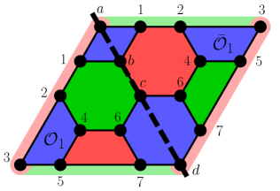
(a)

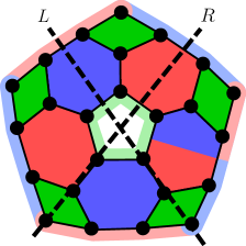
(b)

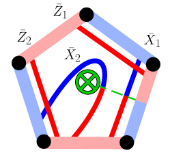
(c)

Figure 15: Surface code patches with symmetry axes (some shown dashed) and with boundary colors indicated. Braiding constituent Majoranas enacts Clifford gates on logical qubits. (a) Patch with one symmetry axis. Braiding equivalently numbered Majoranas across this line results in an encoded Hadamard gate on the logical qubit. (b) Patch with two logical qubits and one logical MZM. This patch has five symmetry axes (the domain wall is a gauge choice, thus does not break this symmetry), two of which are shown and labelled $L$ and $R$. (c) Logical (string) operators for the patch in (b) are schematically illustrated.

VI Fault-Tolerant Gates on Small Majorana Surface Codes

In this penultimate section, we describe another approach to achieving native Clifford gates in the MSC. This method has no analogue in bosonic codes, as it arises from the non-Abelian statistics of constituent Majoranas. Specifically, braiding these Majoranas in the MSC can implement Clifford gates on the logical qubit(s) stored therein. The patches of MSC require one or more lines of mirror symmetry to be suitable for this type of gate. Two examples of these are shown in Figure 15, with the symmetry axes indicated by dashed lines. We require braids to occur across this line of symmetry which, as drawn, are relatively long-range. Hence, this technique would be either suitable for small patches of the MSC or patches that are “folded” along these lines of symmetry to make the braids short-range.

We begin with the code shown in Figure 15a, which stores one logical qubit. We will show that we can enact a single-qubit Clifford gate on this qubit by braiding the constituent Majoranas. Let $U$ be the unitary that braids all Majoranas on opposite sides of the symmetry axis of the code (i.e. those labelled with the same numbers in Figure 15a). That is, $U=\prod_{j=1}^{7}\exp{(\frac{\pi}{4}\bar{\gamma}_{j}\gamma_{j})}$, where $\bar{\gamma}_{j}$ is in the top-right half of the code and $\gamma_{j}$ is in the bottom-left. To see that $U$ implements an encoded Clifford gate, we firstly show that it preserves the stabilizer group. We start with the four-body blue plaquette operators in the bottom-left and top-right corners of the code, which we denote $\mathcal{O}_{1}$ and $\bar{\mathcal{O}}_{1}$ respectively (see Figure 15a). We choose the ordering $\mathcal{O}_{1}=-\gamma_{3}\gamma_{2}\gamma_{4}\gamma_{5}$ and $\bar{\mathcal{O}}_{1}=-\bar{\gamma}_{3}\bar{\gamma}_{2}\bar{\gamma}_{4}\bar{\gamma}_{5}$. Then $U\mathcal{O}_{1}U^{\dagger}=-\bar{\gamma}_{3}\bar{\gamma}_{2}\bar{\gamma}_{4}\bar{\gamma}_{5}=\bar{\mathcal{O}}_{1}$, and similarly $U\bar{\mathcal{O}}_{1}U^{\dagger}=\mathcal{O}_{1}$.

We similarly choose oppositely-oriented plaquette operators between the two halves, so that $U$ maps stabilizer generators to other stabilizer generators under conjugation, without any sign changes. The blue plaquette operators that are intersected by the symmetry axis have their orientations reversed by $U$. In the case of the blue four-body operator in the top-left corner, this results in a change of sign. But it picks up another minus sign because, under conjugation, $U:\gamma_{1}\mapsto\bar{\gamma}_{1}$ and $\bar{\gamma}_{1}\mapsto-\gamma_{1}$. It can similarly be seen that the blue hexagonal plaquette operator does not change its sign under conjugation by $U$. Hence $U$ preserves the whole stabilizer group.

We also define logical operators for the encoded qubit: $\bar{X}=-\gamma_{a}\gamma_{1}\gamma_{2}\gamma_{3}$ and $\bar{Z}=-\gamma_{3}\gamma_{5}\gamma_{7}\gamma_{d}$. Hence $U\bar{X}U^{\dagger}=-\gamma_{a}\bar{\gamma}_{1}\bar{\gamma}_{2}\bar{\gamma}_{3}=\eta\bar{Z}$ and $U\bar{Z}U^{\dagger}=\lambda\bar{X}$, where $\eta,\lambda\in\{+1,-1\}$ depend on the definition of the stabilizer operators. Hence $U=\bar{H}$, the encoded Hadamard operation, up to a logical Pauli operator (set by $\eta$ and $\lambda$).

This operation $U$ is fault-tolerant as it retains the locality of errors. That is, suppose $E\in\text{Maj}(18)$ is an error operator acting on the constituent Majoranas of the code. Then conjugating $E$ with $U$ results in another error operator $E^{\prime}$ with the same weight as $E$. Moreover, we can ensure that $U$ has a very low probability of introducing further errors into the system, since the constituent braids making up $U$ can be made arbitrarily accurate by increasing Majorana separation. In this way we combine the topological protection of constituent braid operations with the protection afforded by the MSC.

A larger set of encoded gates via braids can be found in codes that have more than one axis of symmetry. MSCs defined on the same lattice as stellated color codes [BBrown_Twists_CC], such as the one shown in Figure 15b, have this property. They also possess highly favourable encoding rates among planar code architectures [BBrown_Twists_CC], making them interesting candidates for near-term devices. The code of Figure 15b stores two logical qubits and one logical MZM. (It contains an odd number of constituent Majoranas; this implies that it is part of a larger Majorana system.) The logical operators of the encoded qubits are the string operators indicated in Figure 15c. Let $U_{L}$ (resp. $U_{R}$) denote the operation that braids all constituent Majoranas across the first (resp. second) line of symmetry [labelled $L$ (resp. $R$) in Figure 15b]. One can again show that $U_{L}$ and $U_{R}$ both preserve the stabilizer group. Furthermore, $U_{L}\bar{Z}_{1}U_{L}^{\dagger}=\bar{Z}_{2}$, $U_{L}\bar{Z}_{2}U_{L}^{\dagger}=\bar{Z}_{1}$, $U_{L}\bar{X}_{1}U_{L}^{\dagger}=\bar{Z}_{1}\bar{Y}_{2}$, and $U_{L}\bar{X}_{2}U_{L}^{\dagger}=\bar{Z}_{2}\bar{Y}_{1}$. (Different ordering choices for the logical operators and stabilizers can introduce signs into the above relations.) These transformations are enacted by the following Clifford circuit:

(9)

The braid $U_{R}$ maps $\bar{Z}_{1}\mapsto\bar{Z}_{1}$, $\bar{X}_{1}\mapsto\bar{X}_{1}\bar{X}_{2}$, $\bar{Z}_{2}\mapsto\bar{Z}_{1}\bar{Y}_{2}$ and $\bar{X}_{2}\mapsto\bar{X}_{2}$, up to signs. The Clifford circuit that enacts this gate is the following: Figure 20: Braiding $Z_{3}$ twists results in the following transformations of Pauli operators: (a) $\bar{X}_{1}\mapsto\bar{X}_{2}$, (b) $\bar{Z}_{2}\mapsto\bar{Z}_{1}\bar{X}_{2}$, and (c) $\bar{Z}_{1}\mapsto\bar{Y}_{1}\bar{Y}_{2}$.

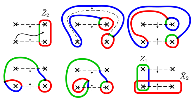
(b)

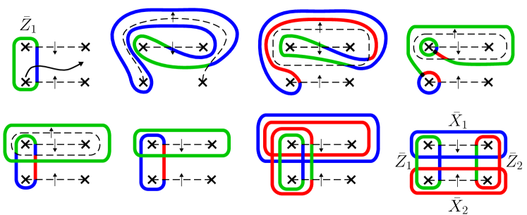
(c)

In Figure VI, we show how braiding two $Z_{3}$ twists in a quartet affects the logical operators $\bar{X}_{1}$, $\bar{Z}_{2}$ and $\bar{Z}_{1}$ for the two BT qubits. The effect on logical operator $\bar{X}_{2}$ is shown in Figure 8 of the main text.

Appendix E Lattice Surgery for Large-Weight Logical MZM Bilinear Measurement

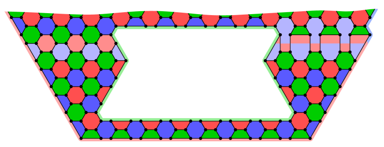
(b)

Figure 21: Procedure for measuring a high-weight logical MZM bilinear, $i\Upsilon_{a}\Upsilon_{b}$. In (a), a small section of surface code patch is shown in the top-half of the figure, with the color of all boundaries indicated. Logical MZMs $\Upsilon_{a}$ and $\Upsilon_{b}$ are supported on odd-length boundaries of color blue and red respectively. Ancilla logical MZMs $\tilde{\Upsilon}_{a}$ and $\tilde{\Upsilon}_{b}$ are supported on blue boundaries. The ancilla patch is prepared in the $+1$ eigenstate of $i\tilde{\Upsilon}_{a}\tilde{\Upsilon}_{b}$. (b) Plaquette operators connecting the surface code patch with the ancilla patch are then measured. The product of light blue plaquettes (left) and four- and six-body plaquettes (right) are the operators $i\Upsilon_{a}\tilde{\Upsilon}_{a}$ and $i\Upsilon_{b}\tilde{\Upsilon}_{b}$ respectively. Once these operators are measured non-destructively, destructive measurement of $i\tilde{\Upsilon}_{a}\tilde{\Upsilon}_{b}$ is performed. The product of the first two measurements gives the measurement outcome of $i\Upsilon_{a}\Upsilon_{b}$ while the final measurement determines the correction operation required.

In Figure E, we illustrate the lattice surgery procedure for measuring the bilinear operator $i\Upsilon_{a}\Upsilon_{b}$, where these two logical MZMs have arbitrarily high weights. In the example, $\Upsilon_{a}$ is supported on a blue boundary and $\Upsilon_{b}$ on a red boundary. Similarly to in Section IV.3.1, we prepare a patch, supporting ancilla logical MZMs $\tilde{\Upsilon}_{a}$ and $\tilde{\Upsilon}_{b}$, in the state $i\tilde{\Upsilon}_{a}\tilde{\Upsilon}_{b}=+1$. These logical MZMs will have a similar weight to $\Upsilon_{a}$ and $\Upsilon_{b}$ respectively, and will be supported on blue boundaries. We measure the extra plaquette operators shown in Figure 21b connecting the two patches. Note that the product of the eigenvalues of those plaquette operators connecting $\Upsilon_{a}$ and $\tilde{\Upsilon}_{a}$ is equal to the eigenvalue of $i\Upsilon_{a}\tilde{\Upsilon}_{a}$, and similarly for $i\Upsilon_{b}\tilde{\Upsilon}_{b}$. We then measure $i\tilde{\Upsilon}_{a}\tilde{\Upsilon}_{b}$ destructively (by measuring all blue bond operators) and perform/track a correction operation dependent on this measurement outcome (cf. Section IV.3.1).

Appendix F Calculating the Correction Operation for Logical Fermion Parity Measurement

Here, we go through the details of Section IV.3.2, specifically showing how to determine the correction operation that needs to be tracked when measuring a logical fermion parity operator.

To determine this operation, we need to assess whether each logical bilinear operator has been preserved by the measurement-based procedure outlined. We deal with the example of $i\Upsilon_{1}\Upsilon_{3}$ specifically. We can use the final column of Table 1 to determine that after the lattice surgery measurements, this bilinear is mapped to $\lambda_{1}\lambda_{3}\bar{Z}_{B}$ (it is unchanged by the final measurement of $i\Upsilon_{4}\tilde{\Upsilon}_{4}$). The final step of the procedure from Section IV.3.2 is to measure all blue bond operators on the ancilla patch, from which we deduce the measurement outcome of operator $\tilde{\Gamma}_{4}$ to be $\eta_{1}$, $i\tilde{\Upsilon}_{1}\tilde{\Upsilon}_{2}\,\bar{X}_{B}$ to be $\eta_{2}$ and $i\tilde{\Upsilon}_{2}\tilde{\Upsilon}_{4}\,\bar{Z}_{B}$ to be $\eta_{3}$. The post-measurement state of the logical qubits can be obtained by acting three logical operators $R_{1}$, $R_{2}$ and $R_{3}$ on the pre-measurement state. This is equivalent to replacing projectors with logical braids in Section IV.3.1.

We now determine $R_{1}$, $R_{2}$ and $R_{3}$ for this example. Note the logical operators stabilizing the pre-measurement state are those that were just measured via lattice surgery: $\lambda_{j}i\Upsilon_{j}\tilde{\Upsilon}_{j}$ for $j=1,2,3,4$. We consider first the measurement of $\tilde{\Gamma}_{4}$ (it does not matter which we choose to consider first, since the measurements all commute). A logical braid that enacts the same transformation as this measurement is (see Section IV.3.1):

$$R_{1} =\exp{\left(\eta_{1}\frac{\pi}{4}\tilde{\Gamma}_{4}i\Upsilon_{1}\tilde{\Upsilon}_{1}\right)}$$ (18)

$$=\exp{\left(i\eta_{1}\frac{\pi}{4}\Upsilon_{1}\tilde{\Upsilon}_{2}\tilde{\Upsilon}_{3}\tilde{\Upsilon}_{4}\right)}.$$ (19)

The measurement operator anti-commutes with all $\lambda_{j}i\Upsilon_{j}\tilde{\Upsilon}_{j}$ and so only products of pairs of these operators will stabilize the post-measurement state. The full list of independent operators stabilizing this state is: $\eta_{1}\tilde{\Gamma}_{4}$, and $\lambda_{1}\lambda_{j}\Upsilon_{1}\Upsilon_{j}\tilde{\Upsilon}_{1}\tilde{\Upsilon}_{j}$ for $j=2,3,4$. Note also that $\Gamma_{4}=\eta_{1}\lambda_{1}\lambda_{2}\lambda_{3}\lambda_{4}$ on the post-measurement state.

We then consider the measurement of $i\tilde{\Upsilon}_{1}\tilde{\Upsilon}_{2}\,\bar{X}_{B}$. This anti-commutes with operators $\lambda_{1}\lambda_{3}\Upsilon_{1}\Upsilon_{3}\tilde{\Upsilon}_{1}\tilde{\Upsilon}_{3}$ and $\lambda_{1}\lambda_{4}\Upsilon_{1}\Upsilon_{4}\tilde{\Upsilon}_{1}\tilde{\Upsilon}_{4}$, so we can choose:

$$R_{2} =\exp{\left(\eta_{2}\lambda_{1}\lambda_{3}\frac{\pi}{4}(i\tilde{\Upsilon}_{1}\tilde{\Upsilon}_{2}\bar{X}_{B})(\Upsilon_{1}\Upsilon_{3}\tilde{\Upsilon}_{1}\tilde{\Upsilon}_{3})\right)}$$ (20)

$$=\exp{\left(\eta_{2}\lambda_{1}\lambda_{3}\frac{\pi}{4}i\tilde{\Upsilon}_{2}\Upsilon_{3}\Upsilon_{1}\tilde{\Upsilon}_{3}\bar{X}_{B}\right)}.$$ (21)

We then have the stabilizing operators: $\eta_{1}\tilde{\Gamma}_{4}$, $\eta_{2}i\tilde{\Upsilon}_{1}\tilde{\Upsilon}_{2}\,\bar{X}_{B}$, $\lambda_{1}\lambda_{2}\Upsilon_{1}\Upsilon_{2}\tilde{\Upsilon}_{1}\tilde{\Upsilon}_{2}$ and $\eta_{1}\lambda_{1}\lambda_{2}\lambda_{3}\lambda_{4}\Gamma_{4}$. Finally we consider the measurement of $i\tilde{\Upsilon}_{2}\tilde{\Upsilon}_{4}\bar{Z}_{B}$. We can choose:

$$R_{3} =\exp\left(\eta_{3}\lambda_{1}\lambda_{2}\frac{\pi}{4}(i\tilde{\Upsilon}_{2}\tilde{\Upsilon}_{4}\bar{Z}_{B})(\Upsilon_{1}\Upsilon_{2}\tilde{\Upsilon}_{1}\tilde{\Upsilon}_{2})\right).$$ (22)

We have the final stabilizing operators: $\eta_{1}\tilde{\Gamma}_{4}$, $\eta_{2}i\tilde{\Upsilon}_{1}\tilde{\Upsilon}_{2}\,\bar{X}_{B}$, $\eta_{3}i\tilde{\Upsilon}_{2}\tilde{\Upsilon}_{4}\,\bar{Z}_{B}$ and $\eta_{1}\lambda_{1}\lambda_{2}\lambda_{3}\lambda_{4}\Gamma_{4}$.

The operator $\lambda_{1}\lambda_{3}\bar{Z}_{B}$ is therefore updated by the measurements to:

$$R_{3}R_{2}R_{1}(\lambda_{1}\lambda_{3}\bar{Z}_{B})R_{1}^{\dagger}R_{2}^{\dagger}R_{3}^{\dagger}=i\eta_{2}\tilde{\Upsilon}_{2}\Upsilon_{3}\Upsilon_{1}\tilde{\Upsilon}_{3}\bar{X}_{B}\bar{Z}_{B}.$$ (23)

We can then multiply this operator by the stabilizers $\eta_{2}i\tilde{\Upsilon}_{1}\tilde{\Upsilon}_{2}\,\bar{X}_{B}$, $\eta_{3}i\tilde{\Upsilon}_{2}\tilde{\Upsilon}_{4}\,\bar{Z}_{B}$ and $\eta_{1}\tilde{\Gamma}_{4}$ to find the operator that acts equivalently on the post-measurement state. This operator is $-\eta_{1}\eta_{3}i\Upsilon_{1}\Upsilon_{3}$. Hence, we find that the bilinear $i\Upsilon_{1}\Upsilon_{3}$ is preserved whenever $-\eta_{1}\eta_{3}=1$. Otherwise, we need to apply/track a correction operation which flips (i.e. anti-commutes with) operator $i\Upsilon_{1}\Upsilon_{3}$.

We do the same for all other bilinear operators. The appropriate correction operation is one that anti-commutes with all bilinears that need to be flipped and commutes with all bilinears that do not need to be flipped.

Appendix G Arbitrary String Operator Measurement Details

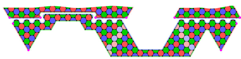
(b)

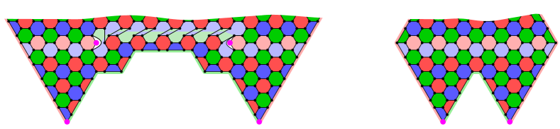
(c)

Figure 22: Example setup for measuring a product of string operators $S_{1}S_{2}$, here represented as red string operators. (a) Ancilla patches host logical MZMs $\tilde{\Upsilon}_{1_{a}}$ and $\tilde{\Upsilon}_{1_{b}}$ (left), $\tilde{\Upsilon}_{c}$ and $\tilde{\Upsilon}_{d}$ (centre), $\tilde{\Upsilon}_{2_{a}}$ and $\tilde{\Upsilon}_{2_{b}}$ (right). (b) Ancilla patches are fused with lattice surgery to measure $i\tilde{\Upsilon}_{1_{b}}\tilde{\Upsilon}_{2_{a}}$. (c) Lattice surgery for measuring $S_{1}(i\tilde{\Upsilon}_{1_{a}}\tilde{\Upsilon}_{1_{b}})$ and $S_{2}(i\tilde{\Upsilon}_{2_{a}}\tilde{\Upsilon}_{2_{b}})$.

Here we extend the procedures of Section IV.5 to measuring arbitrary products of fermionic and bosonic string operators. We assume we wish to measure a product of $k$ operators, labelled $S_{1},\ldots,S_{k}$ and colored either red or blue. We start by introducing $k$ ancilla patches, each hosting two logical MZMs, $\tilde{\Upsilon}_{j_{a}}$ and $\tilde{\Upsilon}_{j_{b}}$ for $j=1,\ldots,k$, and we prepare each patch in the $i\tilde{\Upsilon}_{j_{a}}\tilde{\Upsilon}_{j_{b}}=+1$ state. This also prepares the $+1$ eigenstate of operator $\tilde{\Gamma}=\prod_{j=1}^{k}i\tilde{\Upsilon}_{j_{a}}\tilde{\Upsilon}_{j_{b}}$. An example of this setup is shown in Figure LABEL:subfig:arb_mmt_app_1 for $k=2$. In this example, $S_{1}$ is a bosonic string operator encircling a pair of fermionic twists hosting logical MZMs on blue boundaries. Both $S_{1}$ and $S_{2}$ are red string operators. We then measure $i\tilde{\Upsilon}_{j_{b}}\tilde{\Upsilon}_{(j+1)_{a}}$ for all $j<k$, to entangle these ancilla patches, while preserving the state of $\tilde{\Gamma}$. To achieve this, we can bridge the gap between ancilla patches with another ancilla patch. This is the ancilla patch hosting $\tilde{\Upsilon}_{c}$ and $\tilde{\Upsilon}_{d}$ in Figure LABEL:subfig:arb_mmt_app_1. The measurement of $i\tilde{\Upsilon}_{1_{b}}\tilde{\Upsilon}_{2_{a}}$ is performed via lattice surgery, shown in Figure 22b (see also Section IV.3.1 for an explanation of this procedure). After this measurement, the middle patch hosting $\tilde{\Upsilon}_{c}$ and $\tilde{\Upsilon}_{d}$ is discarded.

We then measure $S_{j}(i\tilde{\Upsilon}_{j_{a}}\tilde{\Upsilon}_{j_{b}})$ for all $j$, using lattice surgery. This does not reveal any information about the individual $S_{j}$ but we can use the fact that $\tilde{\Gamma}=1$ to learn the eigenvalue of $\prod_{j=1}^{k}S_{j}$. This measurement is shown in Figure 22c. Finally we measure $i\tilde{\Upsilon}_{j_{2}}\tilde{\Upsilon}_{(j+1)_{1}}$ for all $j$ once again (with $k+1\equiv 1$), to disentangle the ancilla patches from the code lattice. We can then discard the ancilla patches. Our code patch is left in an eigenstate of $\prod_{j=1}^{k}S_{j}$. We may need to apply/track a correction operation that is dependent on the final ancilla measurements.

Notice that the logical MZMs encircled by $S_{1}$ in the example of Figure G commute with all lattice surgery measurements. Interestingly, there are only bosonic twists present during the lattice surgery phase (see pink dots in Figure 22c) and hence the logical MZMs are temporarily of the form discussed in Appendix LABEL:app:Logical_Maj_Boundary.