Large U(1) charges from flux breaking in 4D F-theory models

Abstract

We study the massless charged spectrum of $\mathrm{U}(1)$ gauge fields in F-theory that arise from flux breaking of a nonabelian group. The $\mathrm{U}(1)$ charges that arise in this way can be very large. In particular, using vertical flux breaking, we construct an explicit 4D F-theory model with a $\mathrm{U}(1)$ decoupled from other gauge sectors, in which the massless/light fields have charges as large as 657. This result greatly exceeds prior results in the literature. We argue heuristically that this result may provide an upper bound on charges for light fields under decoupled $\mathrm{U}(1)$ factors in the F-theory landscape. We also show that the charges can be even larger when the $\mathrm{U}(1)$ is coupled to other gauge groups.

1 Introduction

It is well-known that string theory, when compactified on manifolds in various dimensions, gives a vast range of vacuum solutions known as the string landscape. The low-energy physics of these vacuum solutions can be described by quantum field theories coupled to gravity, with a wide range of different gauge groups and matter content. Nevertheless, there are strong constraints from string theory, or quantum gravity in general, on the low-energy theories that have a consistent UV completion with gravity. Such constraints have been a key component in the analysis of string theory since the early days of the subject, when Green and Schwarz identified the strong conditions imposed by anomaly cancellation on quantum theories of gravity in ten dimensions Green:1984sg , leading to the identification of the heterotic string theory Gross:1984dd ; later work has shown that indeed all consistent theories of quantum gravity in ten dimensions with supersymmetry are those that come from string theory (at least at the level of massless spectra) Adams:2010zy ; Kim:2019vuc .

In lower space-time dimensions, particularly in 4D, the relationship is much less clear between the set of theories that can be realized in string theory and those that appear consistent from the point of view of low-energy EFT coupled to gravity. In recent years, observations of general features of string vacua and black hole behavior have led to a number of speculations regarding quantum gravity constraints on low-energy physics that are often referred to as Swampland Conjectures VafaSwamp ; OoguriVafaSwamp (see vanBeest:2021lhn for a recent review). These constraints have the potential not only to shed light on the general structure of string theory and quantum gravity, but also may have phenomenological implications leading to insights into physics beyond the Standard Model.

One concrete set of questions regarding consistent quantum gravity theories and the string landscape addresses bounds on the complexity of the gauge and matter fields that are possible. For example, while the rank of the gauge group in 6D or 4D supersymmetric string vacua can be very high (see, e.g., Candelas:1997eh ; Aspinwall:1997ye ; MorrisonTaylorToric ; Wang:2020gmi ), there is believed to be a finite bound. Similarly, explicit string constructions of vacua in four and higher dimensions give massless or light matter representations of bounded complexity for nonabelian gauge groups (see, e.g., Dienes:1996yh ; KleversEtAlExotic ; Cvetic:2018xaq ). In this paper we focus on the question of what kinds of charges are possible for massless or light fields charged under a U(1) gauge group in a 4D string vacuum constructed from F-theory VafaF-theory ; MorrisonVafaI ; MorrisonVafaII .

One of the most widely accepted swampland-style conjectures is the Completeness Hypothesis Polchinski:1998rr ; Banks:2010zn , which states that in a gauge theory coupled to gravity, all gauge charges (consistent with charge quantization) must be realized by some physical states. This conjecture has been proven in the context of quantum gravity in AdS space with a holographic dual description Harlow:2018tng . Here the physical states can be massless, or massive including black holes. On the other hand, the situation is less well understood if we consider only massless or light fields. We may expect upper bounds on the gauge charges that can be realized by massless fields in the landscape, but it is not clear how large the upper bounds are or whether the bounds even exist. This is particularly unclear for $\mathrm{U}(1)$ charges since, as explained below, it is very hard to geometrically engineer $\mathrm{U}(1)$ gauge groups with even moderately large charges (i.e., $q>3$) for massless states in string theory.

It is natural to look for such upper bounds using the framework of F-theory, since this approach provides a global description of the largest connected class of supersymmetric string vacua that is currently understood (see WeigandTASI for a review). F-theory gives 4D $\mathcal{N}=1$ supergravity models when compactified on elliptically fibered Calabi-Yau (CY) fourfolds $Y$, corresponding to non-perturbative compactifications of type IIB string theory on general (non-Ricci flat) complex Kähler threefold base manifolds $B$. F-theory is also known to contain many vacua that are dual to many other types of string compactifications, such as heterotic models. The power of F-theory comes from geometrizing the non-perturbative 7-brane backgrounds in type IIB string theory into elliptically fibered manifolds, which can be analyzed using well-established tools in algebraic geometry. Therefore, F-theory allows us to explore the strongly coupled regime of the string landscape. Charge completeness in the context of F-theory is shown in Morrison:2021wuv to follow from some standard assumptions regarding the physical interpretation of the F-theory geometry, for 6D theories and corresponding gauge sectors of 4D theories.

In the F-theory framework, nonabelian gauge groups arise from singularities on divisors (algebraic codimension-one loci) on $B$. In six or more space-time dimensions, the form of the nonabelian part of the gauge group and corresponding massless matter content can be easily determined using the local geometry Kodaira ; Neron ; BershadskyEtAlSingularities ; KatzVafa , which is easy to study. In contrast, $\mathrm{U}(1)$ gauge factors in 6D and 8D F-theory models, as well as in many 4D models, arise from the global geometry. To be precise, these abelian factors in the gauge group arise from a Mordell-Weil group of rational sections with nonzero rank in the elliptic fibration MorrisonVafaII ; AspinwallMorrisonNonsimply ; Aspinwall:2000kf ; Grimm:2010ez . It is much harder to engineer these models, and surprisingly few explicit F-theory constructions have been found with any but the simplest charged matter structure. The best-understood class of models with a single $\mathrm{U}(1)$, known as the Morrison-Park model MorrisonParkU1 , gives a universal form of Weierstrass model with U(1) gauge group and massless (absolute values of) charges $q=1,2$. Explicit models with $q=3,4,5$ have been constructed in KleversEtAlToric ; Raghuram34 ; Knapp:2021vkm respectively, while models with $q=6$ are inferred from the type IIB limit in Cianci:2018vwv , and a procedure for constructing these charges explicitly from universal flops is given in Collinucci:2019fnh . It has also been argued that $q$ can be as large as 21 in 6D F-theory models using implicit Higgsing arguments Raghuram:2018hjn , and an algorithm for computing general U(1) charges from the form of a given Weierstrass model has been developed in Raghuram:2021wvx , but explicit models with $q>6$ are still lacking. On the other hand, it was argued in Taylor:2018khc that there is an infinite swampland of massless $\mathrm{U}(1)$ charge spectra in 6D supergravity theories. In Raghuram:2020vxm , a systematic criterion was proposed for ruling out most of this infinite swampland, as F-theory constructions of these models generally lead to an “automatic enhancement” of the gauge group, and some low-energy arguments for this automatic enhancement were put forth in Cvetic:2021vsw .

Note that we primarily focus in this paper on charges of massless or light fields under isolated $\mathrm{U}(1)$ factors only; more complicated charge structures can arise when there are also nonabelian gauge factors and there are fields that have both $\mathrm{U}(1)$ and nonabelian charges, as discussed in Section 5.

The preceding discussion has focused primarily on 6D F-theory models. While 4D F-theory models can be constructed with similar charges using the same kinds of Weierstrass models described above (Morrison-Park, etc. for charges up to $q=6$), there are also some qualitatively different possibilities in 4D due to the inclusion of flux backgrounds, which can affect the gauge groups and matter content. In particular, with the power of fluxes it becomes possible to build $\mathrm{U}(1)$ gauge groups from the local geometry, which enables us to construct a much larger class of $\mathrm{U}(1)$ models with larger $q$. Indeed, it was noticed in LiFluxbreaking that large $\mathrm{U}(1)$ charges can easily arise through breaking of nonabelian gauge groups using so-called vertical flux (referred to as “vertical flux breaking” henceforth), which will be described below. In this paper, we take this approach. We describe the general framework of F-theory models with $\mathrm{U}(1)$ factors from flux breaking, construct some examples with large charges ($q\gg 6$), and try to identify a plausible upper bound for $q$ in the 4D F-theory landscape.

The strategy is as follows: We first identify nonabelian models that support vertical flux breaking down to a single decoupled $\mathrm{U}(1)$. We can choose an arbitrarily exotic linear combination of the Cartan $\mathrm{U}(1)$’s to be preserved, as long as appropriate vertical flux satisfying all relevant constraints is turned on. This exotic $\mathrm{U}(1)$ is the source of large $q$. As the combination becomes more exotic, more flux is needed to satisfy flux quantization Witten:1996md , and the flux configuration finally hits the tadpole bound Sethi:1996es . These are the only constraints that lead to an upper bound of $q$ for a given geometry. We describe the general framework for this flux breaking and analyze some specific models that give particularly large values of $q$. To maximize $q$, we should maximize the tadpole bound, which is fixed by the Euler characteristic $\chi(\hat{Y})$ of the resolved elliptic Calabi-Yau fourfold $\hat{Y}$ from the F-theory construction. At the same time, the general structure of the intersection form on middle cohomology indicates that we should minimize the intersection numbers on the divisor $\Sigma$ that supports the original nonabelian factor, such that the tadpole caused by a given flux configuration is minimal. As a specific example of the exotic $\mathrm{U}(1)$ charges arise from flux breaking, we construct an explicit 4D F-theory model that combines the two optimizations described above, leading to a surprisingly large value of $q$:

$$q_{\mathrm{max}}=657\,,$$ (1)

for light vector-like charged matter fields. A similar construction can give truly massless chiral matter fields with charges of 465 or greater.

This paper is organized as follows: In Section 2, we review vertical flux and the formalism of vertical flux breaking. The review is brief, only presenting essential facts for our constructions of $\mathrm{U}(1)$ models. We refer the readers to LiFluxbreaking for more details. In Section 3, we go through the general framework of vertical flux breaking from a geometric nonabelian group to an isolated $\mathrm{U}(1)$ gauge factor, and illustrate with a specific class of simple examples from the breaking $\mathrm{SU}(3)\rightarrow\mathrm{U}(1)$. In Section 4, we present the explicit 4D F-theory model with $q_{\mathrm{max}}=657$ for vector-like matter, and related models with comparably large charges for massless chiral fields. The $\mathrm{U}(1)$ model comes from a $G_{2}\rightarrow\mathrm{U}(1)$ breaking on the CY fourfold with the fifth highest $h^{3,1}$ in the Kreuzer-Skarke (KS) database of toric hypersurface constructions Kreuzer:1997zg ; Scholler:2018apc . We describe this model in some detail, and give qualitative arguments for why this model may give, or at least be close to, the upper bound on decoupled $\mathrm{U}(1)$ charges in the 4D F-theory landscape. In Section 5, we extend our discussion to the case of $\mathrm{U}(1)$ coupled to other gauge groups, with an example of even slightly larger $q_{\mathrm{max}}$ when the $\mathrm{U}(1)$ is coupled to an $E_{6}$. We finally conclude in Section 6, and give more geometric properties of our $\mathrm{U}(1)$ model in Appendix A.

2 Formalism of vertical flux breaking

In this section, we review the formalism of breaking nonabelian gauge groups on divisors using vertical flux in 4D F-theory models. As the formalism has been described in depth in LiFluxbreaking , here we only recap the essential facts for our construction of $\mathrm{U}(1)$ models and set up the notation.

2.1 Vertical flux

To describe the flux backgrounds, we first need some basic geometric facts about the compactifications. As mentioned in Section 1, we consider F-theory compactified on a CY fourfold $Y$, which is an elliptic fibration on a threefold base $B$. Nonabelian gauge groups arise when sufficiently high degrees of singularities are developed in the elliptic fibers over divisors on $B$ (denoted by $D_{\alpha}$), called gauge divisors $\Sigma$. When this happens, $Y$ itself is also singular and we need to consider its resolution $\hat{Y}$ such that we can study cohomology and intersection theory. Let the total gauge group be $G$, where $G$ has no $\mathrm{U}(1)$ factors before flux breaking. For clarity of the analysis, in this section we assume that $G$ is a simple nonabelian gauge group, although essentially the same analysis goes through when $G$ has multiple nonabelian factors, as in the cases considered in §4. The nonabelian group $G$ is supported on a gauge divisor $\Sigma$, and the resolution results in exceptional divisors $D_{1\leq{i}\leq\mathrm{rank}(G)}$ in $\hat{Y}$. Their intersection structure matches (up to monodromy for non-simply-laced groups) the Dynkin diagram of $G$, where each exceptional divisor corresponds to a Dynkin node Kodaira ; Neron . By the Shioda-Tate-Wazir theorem shioda1972 ; Wazir , the divisors $D_{I}$ on $\hat{Y}$ are spanned by the zero section $D_{0}$ of the elliptic fibration, pullbacks of base divisors $\pi^{*}D_{\alpha}$ (which we also call $D_{\alpha}$ depending on context), and the exceptional divisors $D_{i}$. Although the choice of resolution is not unique, our analysis and results are clearly resolution-independent Jefferson:2021bid .

Now we are ready to understand fluxes. These are most easily understood by considering the dual M-theory picture of the F-theory models, that is, M-theory compactified on the resolved fourfold $\hat{Y}$ (reviewed in WeigandTASI ). In the M-theory perspective, fluxes are characterized by the three-form potential $C_{3}$ and its field strength $G_{4}=dC_{3}$. The data of $G_{4}$ flux, which can be studied with well-established tools, is sufficient for determining the gauge groups with flux breaking.

In general, $G_{4}$ is a discrete flux that takes values in the fourth cohomology $H^{4}(\hat{Y},\mathbb{R})$. Its quantization condition is given by Witten:1996md

$$G_{4}+\frac{1}{2}c_{2}(\hat{Y})\in H^{4}(\hat{Y},\mathbb{Z})\,,$$ (2)

where $c_{2}(\hat{Y})$ is the second Chern class of $\hat{Y}$. In all the models we consider below, the relevant components in $c_{2}$ are even and we just require that the corresponding components in $G_{4}$ are integer quantized.

Next, to preserve the minimal amount of supersymmetry (SUSY) and stability in 4D, $G_{4}$ must live in the $(2,2)$ part of middle cohomology, i.e., $G_{4}\in H^{2,2}(\hat{Y},\mathbb{R})\cap H^{4}(\hat{Y},\mathbb{Z})$. SUSY also imposes the condition of primitivity Becker:1996gj ; Gukov:1999ya :

$$J\wedge G_{4}=0\,,$$ (3)

where $J$ is the Kähler form of $\hat{Y}$. Typically primitivity is automatically satisfied, but this is not the case when there is vertical flux breaking. In our models, the primitivity condition leads to stabilization of some Kähler moduli, and stabilization within the Kähler cone imposes constraints on $G_{4}$.

We also have the condition of D3-tadpole cancellation for a consistent vacuum Sethi:1996es :

$$\frac{\chi(\hat{Y})}{24}-\frac{1}{2}\int_{\hat{Y}}G_{4}\wedge G_{4}=N_{D3}\in\mathbb{Z}_{\geq 0}\,,$$ (4)

where $\chi(\hat{Y})$ is the Euler characteristic of $\hat{Y}$, and $N_{D3}$ is the number of D3-branes. To preserve SUSY and stability, we require that there are no anti-D3-branes i.e. $N_{D3}\geq 0$. This condition constrains the size of fluxes to a finite number, which, as shown in the next section, also limits the size of $\mathrm{U}(1)$ charges that can be realized.

All the above constraints are satisfied by general fluxes, while the flux breaking in this paper only uses vertical flux, which satisfies extra constraints. To study this, first consider the orthogonal decomposition of the middle cohomology Braun:2014xka :

$$H^{4}(\hat{Y},\mathbb{C})=H^{4}_{\mathrm{hor}}(\hat{Y},\mathbb{C})\oplus H^{2,2}_{\mathrm{vert}}(\hat{Y},\mathbb{C})\oplus H^{2,2}_{\mathrm{rem}}(\hat{Y},\mathbb{C})\,.$$ (5)

Here the summands refer to horizontal, vertical, and remainder fluxes respectively. The vertical subspace is spanned by products of harmonic $(1,1)$-forms (which are Poincaré dual to divisors, denoted by $[D_{I}]$)

$$H^{2,2}_{\mathrm{vert}}(\hat{Y},\mathbb{C})=\mathrm{span}\left(H^{1,1}(\hat{Y},\mathbb{C})\wedge H^{1,1}(\hat{Y},\mathbb{C})\right)\,.$$ (6)

According to Eq. (2), vertical flux should live in the integral vertical subspace $H^{2,2}_{\mathrm{vert}}(\hat{Y},\mathbb{R})\cap H^{4}(\hat{Y},\mathbb{Z})$ (when $c_{2}$ is even). This subspace is in general hard to analyze, hence we only focus on a slightly smaller subspace $H^{2,2}_{\mathrm{vert}}(\hat{Y},\mathbb{Z})$, which is defined as

$$H^{2,2}_{\mathrm{vert}}(\hat{Y},\mathbb{Z}):=\mathrm{span}_{\mathbb{Z}}\left(H^{1,1}(\hat{Y},\mathbb{Z})\wedge H^{1,1}(\hat{Y},\mathbb{Z})\right)\,.$$ (7)

That is, the span of integer multiples of forms $[D_{I}]\wedge[D_{J}]$. This subspace, although it may be smaller than the full integral vertical subspace in general, provides the structure we need for interesting phenomena from flux breaking. We leave the full analysis of integral vertical flux to future work.

Here are some notations for analyzing vertical flux. We expand

$$G_{4}^{\mathrm{vert}}=\phi_{IJ}[D_{I}]\wedge[D_{J}]\,,$$ (8)

and work with integer flux parameters $\phi_{IJ}$. We will specify the basis for the expansion later. Next, we denote the integrated flux as Grimm:2011fx

$$\Theta_{\Lambda\Gamma}=\int_{\hat{Y}}G_{4}\wedge[\Lambda]\wedge[\Gamma]\,,$$ (9)

where $\Lambda,\Gamma$ are arbitrary linear combinations of $D_{I}$, and subscripts $0,i,\alpha$ refer to the basis divisors $D_{0},D_{i},D_{\alpha}$. In this paper, we use the following resolution-independent formula to relate $\Theta_{i\alpha}$ to $\phi_{i\alpha}$ Grimm:2011sk ; Jefferson:2021bid :

$$\Theta_{i\alpha}=-\kappa^{ij}\Sigma\cdot D_{\alpha}\cdot D_{\beta}\phi_{j\beta}\,,$$ (10)

where $\kappa^{ij}$ is the inverse Killing metric of $G$, and “dots” denote the intersection product. This is the same as the Cartan matrix of $G$ for ADE groups, but in general it is not. Note that in our examples, the only nonzero flux parameters have indices of type $\phi_{j\alpha}$. In general, many gauge groups also admit fluxes of type $\phi_{ij}$ associated with chiral matter of the nonabelian gauge group. The integrated fluxes $\Theta_{j\alpha}$ can also be affected by these parameters, in a fashion that also seems to have a resolution-independent description Jefferson:2021bid , although we will not use such fluxes here.

Now we write down the extra flux constraints satisfied by vertical flux. First, to preserve Poincaré symmetry after dualizing from M-theory, we require Dasgupta:1999ss

$$\Theta_{0\alpha}=\Theta_{\alpha\beta}=0\,.$$ (11)

If the whole $G$ is preserved, a necessary condition is that

$$\Theta_{i\alpha}=0\,,$$ (12)

for all $i,\alpha$. This condition is also sufficient when there is no nontrivial remainder flux. Vertical flux breaking occurs when this condition is violated, which we will discuss next. Note that the violation does not affect the condition in Eq. (11).

2.2 Vertical flux breaking

With the knowledge of vertical flux, we now describe the breaking of geometric gauge groups with vertical flux, or vertical flux breaking. This kind of breaking has been used as early as BeasleyHeckmanVafaI (see also WeigandTASI ), and is recently developed in depth in LiFluxbreaking . In this paper, we only list the results essential for our analysis on $\mathrm{U}(1)$ models, and we refer readers to LiFluxbreaking for full technical details. Note that flux breaking can also be done with remainder flux Buican:2006sn ; BeasleyHeckmanVafaII , but as noted in LiFluxbreaking , vertical flux should be used to realize exotic $\mathrm{U}(1)$ charges.

Recall that we need $\Theta_{i\alpha}=0$ for all $i,\alpha$ to preserve the whole $G$. Now we break $G$ into a smaller group $G^{\prime}$ by turning on some nonzero $\phi_{i\alpha}$. Such flux breaks some of the roots in $G$. It also induces masses for some Cartan gauge bosons by the Stückelberg mechanism Grimm:2010ks ; Grimm:2011tb , hence breaks some combinations of Cartan $\mathrm{U}(1)$’s in $G$. Let $\alpha_{i}$ be the simple roots of $G$, and $T_{i}$ be the Cartan generators associated with $\alpha_{i}$ i.e. in the co-root basis. The root $b_{i}\alpha_{i}$ is preserved under the breaking if

$$\sum_{i}b_{i}\left<\alpha_{i},\alpha_{i}\right>\Theta_{i\alpha}=0\,,$$ (13)

for all $\alpha$. Here $\left<.,\,.\right>$ denotes the inner product of root vectors. Moreover, the corresponding linear combination of Cartan generators

$$\sum_{i}b_{i}\left<\alpha_{i},\alpha_{i}\right>T_{i}\,,$$ (14)

is preserved. These generators form a nonabelian gauge group $G^{\prime}\subset G$ after breaking.

There are additional constraints on vertical flux breaking coming from primitivity, since Eq. (3) is not automatically satisfied when there is vertical flux breaking and $\Theta_{i\alpha}\neq 0$ for some $i,\alpha$. In particular, primitivity requires that

$$\int_{\hat{Y}}[D_{i}]\wedge J\wedge G_{4}=0\,,$$ (15)

which is true only for specific choices of $J$ when there is vertical flux breaking. As a result, the condition of primitivity stabilizes some but not all Kähler moduli in $J$. As discussed in LiFluxbreaking , in the presence of flux breaking, there is a nontrivial condition on the $\alpha$ components of $J$ (in an expansion $J=t^{I}[D_{I}]$ in $\hat{Y}$) that must be satisfied to ensure a nontrivial solution of Kähler moduli, which can be described as follows: Let $r$ be the number of linearly independent $D_{\alpha}$’s appearing in the set of all homologically independent surfaces in the form of $S_{i\alpha}=D_{i}\cdot D_{\alpha}$ (for any $i$ of the given $G$). Now consider the ($r$ $\times$ $\mathrm{rank}(G)$) matrix $\Theta_{(\alpha_{a})(i)}$ (where $a$ and $i$ are the indices for rows and columns respectively). The condition (15) asserts that $t^{\alpha}\Theta_{\alpha i}=0$. Since the solution to primitivity thus requires a nontrivial left null space of the matrix, the rank of the matrix is at most $r-1$. Moreover from Eq. (13), the rank of the matrix is also the change in rank of $G$ during flux breaking. Therefore, we require

$$r\geq\mathrm{rank}(G)-\mathrm{rank}(G^{\prime})+1\,.$$ (16)

In particular, when remainder flux breaking is not available, and all divisors in $\Sigma$ descend from intersections in $B$, we have $r=h^{1,1}(\Sigma)$. This condition limits the availability of vertical flux breaking, which plays an important role in the analysis below. There are still additional sign constraints on the fluxes in order to stabilize the Kähler moduli within the Kähler cone. These constraints will be explicitly demonstrated in examples below.

The above vertical flux generically also induces chiral matter charged under $G^{\prime}$ if $G^{\prime}$ (regardless of $G$) supports chiral matter. In this paper, we focus on cases where matter is charged under a single simple nonabelian gauge group $G$, and $G$ does not support chiral matter. Then the chiral indices are given by the following: for a weight $\beta=-b_{i}\alpha_{i}$ in a representation $R$ of $G$ that is localized on the matter curve $C_{R}=\Sigma\cdot D_{R}$, by analysis following Braun_2012 ; Marsano_2011 ; KRAUSE20121 ; Grimm:2011fx the chiral index is

$$\chi_{\beta}=\sum_{i}b_{i}\frac{\left<\alpha_{i},\alpha_{i}\right>}{\left<\alpha_{\mathrm{max}},\alpha_{\mathrm{max}}\right>}\Theta_{iD_{R}}\,,$$ (17)

where $\alpha_{\mathrm{max}}$ is the longest $\alpha_{i}$. If $R$ is the adjoint localized on the bulk of $\Sigma$, we should replace $C_{R}$ by the canonical class $K_{\Sigma}$ i.e. $D_{R}=K_{B}+\Sigma$ by adjunction.

In addition to nonabelian gauge factors, flux breaking can also give rise to $U(1)$ gauge factors, either in combination with nonabelian factors as studied in LiFluxbreaking , or in isolation. The latter situation is the main focus of this work.

3 Flux breaking to $\mathrm{U}(1)$

We now turn to abelian $\mathrm{U}(1)$ factors in $G^{\prime}$, which are a key feature of vertical flux breaking. We start by giving the general framework for flux breaking of a simple nonabelian factor to $\mathrm{U}(1)$ and then give a simple illustrative example of breaking $\mathrm{SU}(3)\rightarrow\mathrm{U}(1)$ using vertical fluxes.

3.1 $\mathrm{U}(1)$ factors from flux breaking

Although every root of a simple Lie algebra corresponds to a linear combination of Cartan generators, the reverse is seldom true. In fact, we can write down arbitrary linear combinations of Cartan generators, while there is only a finite number of roots. Following the logic of vertical flux breaking described in §2.2, suppose that we have an F-theory model over a threefold base $B$ that contains a single nonabelian gauge factor $G$. We then turn on vertical flux parameters $\phi_{j\beta}$ giving some non-vanishing fluxes $\Theta_{i\alpha}$ through Eq. (10). If we impose the condition (summing as above by convention over doubled indices $i$)

$$p_{i}\Theta_{i\alpha}=0\,,$$ (18)

for all $\alpha$, while

$$\sum_{i}p_{i}\left<\alpha_{i},\alpha_{i}\right>^{-1}\alpha_{i}\,,$$ (19)

is not along any roots, then the Cartan generator

$$p_{i}T_{i}\,,$$ (20)

is preserved but does not belong to any nonabelian subgroup of $G$. Such generators thus form the abelian part of the preserved gauge group $G^{\prime}$. More generally, there may be $\mathrm{U}(1)$’s that are combinations of Cartan generators from multiple gauge factors. These $\mathrm{U}(1)$’s, however, are not relevant to our analysis below, and we focus on $\mathrm{U}(1)$’s coming from $G$ with a single simple nonabelian factor as above. We focus attention in particular on cases involving vertical flux breaking of such a gauge group $G$, where no nonabelian gauge factor remains and we have a single residual $\mathrm{U}(1)$ gauge factor on the gauge divisor. As long as Eq. (18) is satisfied, the coefficients $p_{i}$ look arbitrary and the resulting $\mathrm{U}(1)$ can naively be arbitrarily complicated, which leads to arbitrarily exotic matter, although as we shall discuss there are upper bounds from other flux constraints. This feature gives great power for building $\mathrm{U}(1)$ models from vertical flux breaking, as one can flexibly tune suitable $p_{i}$ to get a desired $\mathrm{U}(1)$, with specific matter content. In contrast, in field theory for example, the $\mathrm{U}(1)$ realized after breaking through a Higgsing process is determined by the representation and vev of the Higgs field, which substantially constrains the resulting possible $\mathrm{U}(1)$ factors and associated charges. While these kinds of Higgsed $\mathrm{U}(1)$ fields are transparent from the low-energy physics point of view, they are much harder to study in general in F-theory as they involve deformations of the Weierstrass model that are in some cases unknown Raghuram:2018hjn . In contrast, vertical flux breaking seems to rely much on the UV physics of string theory, and while we have a clear way of analyzing these systems from the geometry of fluxes, so far we do not see any clear approach to attaining a low-energy description of the breaking.

The condition in Eq. (16) also holds for $\mathrm{U}(1)$ factors. Now $\mathrm{rank}(G^{\prime})$ also counts the number of $\mathrm{U}(1)$’s that descend from $G$. In particular, to break a high-rank nonabelian factor to a single $\mathrm{U}(1)$, the gauge factor must arise on a divisor with $h^{1,1}(\Sigma)\geq\mathrm{rank}(G)$.

3.2 A simple example: breaking $\mathrm{SU}(3)\rightarrow\mathrm{U}(1)$

It is useful to demonstrate the above techniques with a simple example of $\mathrm{U}(1)$ models before discussing the maximization of $\mathrm{U}(1)$ charges. Let us consider the base $B$ as a $\mathbb{P}^{1}$-bundle over $\mathbb{F}_{0}=\mathbb{P}^{1}\times\mathbb{P}^{1}$, with an $\mathrm{SU}(3)$ supported on $\mathbb{F}_{0}$. Notice that $\mathrm{SU}(3)$ has rank $2$ and $h^{1,1}(\mathbb{F}_{0})=2$. Therefore by Eq. (16), $B$ is the simplest base that supports the breaking to $\mathrm{U}(1)$ described in the last subsection. Since the models in the coming sections have the same divisor geometry, this subsection also serves as a warm-up exercise for those constructions.

First, we describe the geometry of $B$. Let the two $\mathbb{P}^{1}$’s on $\mathbb{F}_{0}$ be $s,f$. Then $B$ has three independent divisors: $\Sigma$ as the section $\mathbb{F}_{0}$, and $S,F$ as the $\mathbb{P}^{1}$ bundles on $s,f$ respectively. $\Sigma$ is also the gauge divisor. The only nontrivial intersection number is $\Sigma\cdot S\cdot F=1$. Generically there are (anti-)fundamentals $\mathbf{3}$ and $\bar{\mathbf{3}}$, as well as the adjoint $\mathbf{8}$ as the matter content of the model.

Eq. (16) tells us that we can at most reduce the rank of the gauge group by one when satisfying primitivity. In other words, to preserve at least a $\mathrm{U}(1)$, the nonzero vertical flux should always satisfy the constraint

$$a\Theta_{1\alpha}+b\Theta_{2\alpha}=0\,,$$ (21)

for all $\alpha=S,F$, where $1,2$ are the Cartan indices for $\mathrm{SU}(3)$, and $a,b$ are some coprime integers. There are two possible cases: for generic $a,b$ we obtain the breaking $\mathrm{SU}(3)\rightarrow\mathrm{U}(1)$, but if $a=0$, $b=0$, or $a=b$, these coefficients align with some roots of $\mathrm{SU}(3)$ and we get $\mathrm{SU}(3)\rightarrow\mathrm{SU}(2)$ instead. We focus on the former case with the $\mathrm{U}(1)$ generator $T=aT_{1}+bT_{2}$. The flux constraint is then solved by

$$\left(\phi_{1S},\phi_{2S},\phi_{1F},\phi_{2F}\right)=\frac{1}{3}\left(\left(a-2b\right)n_{S},\left(2a-b\right)n_{S},\left(a-2b\right)n_{F},\left(2a-b\right)n_{F}\right)\,,$$ (22)

where $n_{S},n_{F}$ are flux parameters to be chosen, such that all $\phi$’s are integers to satisfy flux quantization.

Now we turn to the condition of primitivity. In the F-theory limit where the elliptic and exceptional fibers shrink to zero volume, only the Kähler form of $\Sigma$ contributes in Eq. (15). Let the Kähler form of $\Sigma$ be

$$[J_{\Sigma}]=t_{1}\Sigma\cdot F+t_{2}\Sigma\cdot S\,,$$ (23)

where $t_{1},t_{2}$ are Kähler moduli. Eq. (15) then implies

$$t_{1}n_{S}+t_{2}n_{F}=0\,.$$ (24)

To ensure stabilization within the Kähler cone where $t_{1},t_{2}>0$, we require $n_{S},n_{F}$ to be both nonzero and have opposite signs.

Assuming the tadpole constraint (4) is satisfied, now we are free to choose the parameters $a,b,n_{S},n_{F}$ and calculate the resulting $\mathrm{U}(1)$ charges. First notice that under the breaking, the (anti-)fundamentals give charges $a,b,a-b$ and their conjugates, and the adjoint gives charges $a+b,a-2b,2a-b$ and their conjugates. As an example with small flux parameters, let us choose $(a,b,n_{S},n_{F})=(-2,5,2,-1)$. Then we obtain the following spectrum:

$$q=2,\,3,\,5,\,7,\,9,\,12\,.$$ (25)

To be more precise, we can also calculate the chiral spectrum of these charges. Using Eq. (17), we see that the chiral spectrum induced from the adjoint is

$$14\times\mathbf{1}_{3}+4\times\mathbf{1}_{12}+10\times\mathbf{1}_{-9}\,.$$ (26)

It is easy to check that this chiral spectrum is free of both pure gauge and gauge-gravity anomalies since $\sum q_{i}=\sum q_{i}^{3}=0$. More generally, for any such $a,b$, we have the following chiral spectrum from the adjoint:

$$2(b-a)\times\mathbf{1}_{a+b}+2a\times\mathbf{1}_{a-2b}+2b\times\mathbf{1}_{2a-b}\,,$$ (27)

which is remarkably always anomaly-free. One can perform a similar analysis for the (anti-)fundamentals, although it depends more on the geometry of $B$.

Notice that the charges are coprime. Therefore through such a simple construction, we already obtain some relatively large $\mathrm{U}(1)$ charges. In the next Section, we will optimize this procedure subject to the tadpole constraint, to obtain our extremal result $q_{\mathrm{max}}=657$.

Some relevant comments can be made here regarding the connection of these spectra with related 6D models. The family of models described in Eq. (27) is very similar in structure to an infinite family of 6D U(1) models with arbitrarily large charges encountered in Taylor:2018khc . In the 6D case, charges arise from complicated Weierstrass models (see, e.g., Raghuram:2021wvx ), and the infinite family is apparently rendered unphysical by the automatic enhancement mechanism Raghuram:2020vxm ; Cvetic:2021vsw , which guarantees the appearance of an additional U(1) factor. In the 4D case, the charges arise from the distinct physical mechanism of flux breaking, so the infinite family of anomaly-consistent models is bounded by the tadpole, and automatic enhancement does not seem to occur. It would be interesting to better understand how the automatic enhancement story differs in this context. It is also interesting to observe that because $a,b$ are coprime, this family of models can contain massless or light matter fields that generate the full charge lattice, in accord with the massless charge sufficiency conjecture formulated for 6D F-theory in Morrison:2021wuv . In this case, however, the nonzero multiplicities of massless or light matter depend upon the choice of flux. It would be interesting to look further into the question of whether the light fields always generate the full charge lattice for arbitrary choices of flux.

4 A $\mathrm{U}(1)$ model with $q_{\mathrm{max}}=657$

In this section, we construct a $\mathrm{U}(1)$ model with $q_{\mathrm{max}}=657$ using vertical flux breaking. We describe the geometry of the fourfold $\hat{Y}$ and the base $B$, as well as the vertical flux background in detail. Then we give qualitative and heuristic arguments towards $q_{\mathrm{max}}=657$ being (close to) an upper bound in the 4D F-theory landscape. Notice that there are other nonabelian gauge factors in this model, but they are completely decoupled from the $\mathrm{U}(1)$ we construct, hence we still call it a $\mathrm{U}(1)$ model, and the analysis of §3 applies essentially unchanged.

It is useful to first recap our strategy. From Eq. (18), we see that the more exotic the $\mathrm{U}(1)$ or the coefficient $p_{i}$ is, the larger integer $\phi_{i\alpha}$ we need to turn on. From Eq. (4), the size of $\phi_{i\alpha}$ is bounded from above by the Euler characteristic $\chi(\hat{Y})$ and the intersection numbers on $\Sigma$ that arise in $[G_{4}]\cdot[G_{4}]$. Therefore to obtain the largest $q_{\mathrm{max}}$, we shall maximize $\chi(\hat{Y})$ while minimizing the intersection numbers on $\Sigma$. Although the list of elliptic CY fourfolds is far from complete, the KS database provides a set of good toric representatives especially at large $\chi$. Scanning through the KS database leads us to consider the CY fourfold with the fifth largest $h^{3,1}$ and $\chi$. We now describe its geometry in detail.

4.1 Geometry

The fourfold $\hat{Y}$ has the following Hodge numbers:

$$h^{1,1}=256\,,\quad h^{2,1}=0\,,\quad h^{3,1}=289384\,,$$

$$h^{2,2}=44+4h^{1,1}-2h^{2,1}+4h^{3,1}=1158604\,,$$

$$\chi=6(8+h^{1,1}-h^{2,1}+h^{3,1})=1737888\,.$$ (28)

Notice that there are many more fourfolds with the same $\chi$, but they all have much larger $h^{1,1}$ and are harder to analyze, while they very probably do not give larger $q_{\mathrm{max}}$, as discussed in Section 4.3.

$\hat{Y}$ is a CY hypersurface in an ambient toric fivefold, a (singular) weighted projective space $\mathbb{P}^{1,80,492,1148,1722}$ Scholler:2018apc . It can also be understood as a generic elliptic fibration over a toric base $B$ to be specified below. The equivalence of the two descriptions is shown in Appendix A. Now, $B$ can be described as a $B_{2}$-bundle over $\mathbb{P}^{1}$, where $B_{2}$ is a toric surface characterized by a closed cycle of divisors (or rays in the 2D toric fan) with self-intersection numbers $0,6,-12//-11//-12//-12//-12//-12//-12//-12//-12$, where $//$ represents the chain $-1,-2,-2,-3,-1,-5,-1,-3,-2,-2,-1$ MorrisonTaylorToric ; TaylorWangVacua . Its toric rays $v_{\alpha}\in\mathbb{Z}^{2}$ can be taken to be

$$v_{1}=\left(-1,-12\right)\,,\quad v_{2}=\left(0,1\right)\,,\quad...\,,\quad v_{99}=\left(0,-1\right)\,,$$ (29)

where the intermediate rays are determined by $v_{\alpha-1}+v_{\alpha+1}+C_{\alpha}^{2}v_{\alpha}=0$ and $C_{\alpha}^{2}$ is the self-intersection number of the divisor corresponding to $v_{\alpha}$, starting at $C_{1}^{2}=0,C_{2}^{2}=6$. Then the 3D toric fan of $B$ is given by the rays $w_{\alpha}$:

$$w_{0}=\left(0,0,1\right)\,,\quad w_{1\leq\alpha\leq 99}=\left(v_{\alpha},0\right)\,,\quad w_{100}=\left(80,468,-1\right)\,,$$ (30)

where $(80,468)=4v_{19}$ is the twist of the $B_{2}$-bundle. We denote the corresponding divisor classes to be $D^{\alpha}$, where the superscript integer indexing the base divisors is distinguished from the subscript for exceptional divisors as mentioned above; when we use $\alpha$ as a subscript where Cartan indices $i$ are also possible, as in, e.g., $S_{i\alpha}$ we use non-integer notation for the $\alpha$’s. The cones of the fan are given by $\left(w_{0},w_{\alpha},w_{\alpha+1}\right),\left(w_{100},w_{\alpha},w_{\alpha+1}\right)$ for $1\leq\alpha\leq 98$, as well as $\left(w_{0},w_{99},w_{1}\right),\left(w_{100},w_{99},w_{1}\right)$.

The local geometry on divisor $D^{0}=D^{100}$ is clearly $B_{2}$, while that on divisors $D^{1\leq\alpha\leq 99}$ are all Hirzebruch surfaces $\mathbb{F}_{n}$. In particular, we have $h^{1,1}(D^{1\leq\alpha\leq 99})=2$. The intersection numbers on $D^{1\leq\alpha\leq 99}$ are then determined by $n$ only. Note that since the twist is along $v_{19}$, the local geometry on $D^{19}$ is $\mathbb{F}_{0}$, which has the smallest intersection numbers among all $\mathbb{F}_{n}$.

Some of the divisors $D^{1\leq\alpha\leq 99}$ have sufficiently negative normal bundles in $B$ that the elliptic fibration is forced to be singular to certain degrees, and nonabelian gauge factors automatically arise on these divisors. Such rigid or geometrically non-Higgsable gauge groups are present throughout the whole set of moduli space branches associated with elliptic CY ’s over such a base MorrisonTaylorClusters ; MorrisonTaylor4DClusters . As a result, these gauge groups cannot be broken by any geometric deformation (corresponding to Higgsing from the low-energy perspective), while they can still be broken by fluxes. The method for determining the rigid gauge groups in 4D F-theory models has been described in MorrisonTaylor4DClusters , and here we summarize the result applied in this type of case where the base $B$ is a $B_{2}$ bundle over $\mathbb{P}^{1}$. The divisor $D^{1\leq\alpha\leq 99}$ supports $E_{8}$ if $C_{\alpha}^{2}=-11,-12$, $F_{4}$ if $C_{\alpha}^{2}=-5$, $G_{2}$ if $C_{\alpha}^{2}=-3$, and $\mathrm{SU}\left(2\right)$ if $C_{\alpha}^{2}=-2$ and intersects with a $G_{2}$ gauge divisor. Therefore, the full gauge group is

$$E_{8}^{9}\times F_{4}^{8}\times\left(G_{2}\times\mathrm{SU}\left(2\right)\right)^{16}\,.$$ (31)

In particular, there is a $G_{2}$ factor supported on $D^{19}$.

Note that there may be codimension-2 $(4,6)$ singularities localized on divisors supporting $E_{8}$ factors. By computing the normal bundles on divisors, one can check that there are four irreducible components of codimension-2 $(4,6)$ loci on $D^{3}$ (with $C_{3}^{2}=-12$) and one on $D^{15}$ (with $C_{15}^{2}=-11$). To remove these singularities, non-toric blowups must be performed, contributing $5$ to the $h^{1,1}$ in Eq. (4.1). These singularities are associated with extra strongly coupled (probably conformal) sectors that have not been well understood HeckmanMorrisonVafa ; DelZotto:2014hpa ; Apruzzi:2018oge . Nevertheless, these sectors are decoupled from the gauge sectors we are studying and should not affect our analysis.

4.2 Flux background

Now we would like to break some gauge factors in Eq. (31) to get an exotic $\mathrm{U}(1)$ using vertical flux breaking. Since vertical flux breaking must decrease the rank of the gauge group, we cannot have breaking like $\mathrm{SU}(2)\rightarrow\mathrm{U}(1)$. By Eq. (16) with $r=2$ for all gauge factors, we then see that the only available breaking is $G_{2}\rightarrow\mathrm{U}(1)$. One may naively consider a breaking like $G_{2}\times\mathrm{SU}(2)\rightarrow\mathrm{U}(1)$ where the $\mathrm{U}(1)$ is a combination of Cartan generators from both gauge factors, since a $G_{2}$ gauge divisor always intersects with an $\mathrm{SU}(2)$ gauge divisor. It can be shown that, however, such breaking violates an analogous version of Eq. (16).

Here we reach one of the main points in this section: we can minimize the intersection numbers on the gauge divisor by performing the flux breaking on $D^{19}$, which is locally $\mathbb{F}_{0}$ and supports a $G_{2}$. This crucial feature is why we study the fifth largest $h^{3,1}$ and $\chi$ in the KS database but not one of the CY ’s with even larger $\chi$.

Let us specify more details on $D^{19}$. The only $D^{i}$’s that intersect with $D^{19}$ are $D^{0}=D^{100},D^{18},D^{20}$. The curves on $D^{19}$ are then spanned by $D^{0}\cdot D^{19}=D^{100}\cdot D^{19}$ and $D^{18}\cdot D^{19}=D^{20}\cdot D^{19}$. Following the notation in Section 3.2, we denote $\Sigma=D^{19},S=D^{0},F=D^{18}$. The only nontrivial intersection number on $\Sigma$ is $\Sigma\cdot S\cdot F=1$. Now to break $G_{2}\rightarrow\mathrm{U}(1)$, we turn on nonzero $\phi_{i\alpha}$ such that

$$a\Theta_{1\alpha}+b\Theta_{2\alpha}=0\,,$$ (32)

for all $\alpha=S,F$, where the index $i$ is the Cartan index for the $G_{2}$, and integers $a,b$ are coprime. The labels $1,2$ correspond to

$$\kappa^{ij}=\left(\begin{array}[]{cc}6&-3\\ -3&2\end{array}\right)\,.$$ (33)

If $(a,b)$ is not along any root of $G_{2}$, all the roots of $G_{2}$ are broken and the remaining gauge group is $\mathrm{U}(1)$ with generator $T=aT_{1}+bT_{2}$. The flux constraint is solved by

$$\left(\phi_{1S},\phi_{2S},\phi_{1F},\phi_{2F}\right)=\left(\left(a-2b/3\right)n_{S},\left(2a-b\right)n_{S},\left(a-2b/3\right)n_{F},\left(2b-a\right)n_{F}\right)\,,$$ (34)

where $n_{S},n_{F}$ are flux parameters to be chosen. To satisfy flux quantization, we see that $n_{S},n_{F}$ must be multiples of 3 unless $b$ is a multiple of 3. When $b$ is a multiple of 3, one can show that $(a-2b/3)$ and $(2a-b)$ must be coprime and $n_{S},n_{F}$ must be integer. Since the size of $\phi$ has been bounded, to ensure the most exotic choice of $(a,b)$ we should assume $b$ as a multiple of 3 and integer $n_{S},n_{F}$. Now we turn to primitivity; as in Section 3.2, only the Kähler form of $D^{19}$ contributes in Eq. (15) with $D_{i}$ being the exceptional divisors from the $G_{2}$. Therefore, we require $n_{S},n_{F}$ to be both nonzero and have opposite signs.

With the above information, we can easily calculate the tadpole from this flux:

$$\frac{1}{2}\int_{\hat{Y}}G_{4}\wedge G_{4}=-2\left(a^{2}-ab+\frac{b^{2}}{3}\right)n_{S}n_{F}\,.$$ (35)

We see that to minimize the tadpole and satisfy primitivity, we should choose e.g. $(n_{S},n_{F})=(1,-1)$. This ensures the tadpole to be positive. Then Eq. (4) becomes

$$a^{2}-ab+\frac{b^{2}}{3}\leq 36206\,.$$ (36)

To maximize the $\mathrm{U}(1)$ charges, we should choose $(a,b)$ such that the above is the closest to saturation. The ratio between $a$ and $b$ is now determined by the matter spectrum charged under the $G_{2}$. Let us first focus on the adjoint $\mathbf{14}$ of $G_{2}$. After the breaking, the W-bosons become charged singlets with the $\mathrm{U}(1)$ charges

$$a,\,b,\,3a-b,\,2a-b,\,a-b,\,3a-2b\,,$$ (37)

and their conjugates. There are also two uncharged singlets. To find out the largest possible $q_{\mathrm{max}}$, we then maximize one of the charges in the above, subject to the tadpole constraint and the assumption of $b$ being multiple of 3. It turns out that there are multiple choices giving the same largest $q_{\mathrm{max}}$. For example, $(a,b)=(329,657)$ (or $(\phi_{1S},\phi_{2S})=(-109,1)$) gives the largest $b=657$, with the full set of $\mathrm{U}(1)$ charges from the adjoint being

$$q=1,\,327,\,328,\,329,\,330,\,657\,.$$ (38)

Therefore, we have reached one of the main results of this paper, a $\mathrm{U}(1)$ 4D F-theory model with

$$q_{\max}=657\,.$$ (39)

To complete the discussion, we still need to look at other representations. There is also bifundamental matter $(\mathbf{7},\mathbf{2})$ charged under $G_{2}\times\mathrm{SU}(2)$ before breaking MorrisonTaylorClusters . It breaks into representations of $\mathrm{SU}(2)\times\mathrm{U}(1)$ after the breaking, so the $\mathrm{U}(1)$ is still coupled to other gauge factors. One can, however, turn on one more unit of vertical flux to break the adjacent $\mathrm{SU}(2)$ completely. Then the bifundamental also breaks into $\mathrm{U}(1)$ charged singlets and the $\mathrm{U}(1)$ we constructed is fully decoupled. The same calculation as above shows that the bifundamental only gives a subset of $\mathrm{U}(1)$ charges coming from the adjoint, with the maximum being $q=329$.

It is informative to study the chiral spectrum of these large charges. Interestingly, Eq. (17) implies that the chiral indices from the adjoint are proportional to $(n_{S}+n_{F})$, hence vanish in the above example. In particular, it means that the charge $q=657$ must belong to vector-like matter, which is not exactly massless if including interactions in the superpotential. A careful calculation using the approach of BeasleyHeckmanVafaI shows that the multiplicity of vector-like $\mathbf{1}_{657}$ in this model is indeed nonzero. On the other hand, there is chiral matter from the bifundamental. Since the adjacent $\mathrm{SU}(2)$ is completely broken, we can effectively consider two copies of $\mathbf{7}$ localized on $C_{\mathbf{7}}=D^{18}\cdot D^{19}=\Sigma\cdot F$. Eq. (17) then gives the following chiral spectrum:

$$438\times\mathbf{1}_{1}+220\times\mathbf{1}_{-328}+218\times\mathbf{1}_{329}\,,$$ (40)

which is again anomaly-free as expected. Therefore, if we restrict to the truly massless chiral fields only, $q_{\mathrm{max}}$ is not as large as 657. There are still ways to go beyond $q=329$ for chiral fields. For example, in the same model as above, we can choose $(n_{S},n_{F})=(2,-1)$ instead. Then there are chiral fields from the adjoint, and the same calculation of $q_{\mathrm{max}}$ from the adjoint gives $q_{\mathrm{max}}=465\simeq 657/\sqrt{2}$.

One may naively expect, from the low-energy perspective, that we can give the above massless chiral fields a vacuum expectation value to Higgs the symmetry to a discrete abelian group $\mathrm{U}(1)\rightarrow\mathbb{Z}_{k}$. The above example then suggests that $k$ could be as large as 465 for such discrete symmetries in 4D. This is much larger than the largest size $\mathbb{Z}_{6}$ currently known (Anderson:2019kmx and references therein) for discrete gauge symmetries from Tate-Shafarevich/Weil-Châtelet groups of smooth elliptic CY threefolds or fourfolds Braun:2014oya ; Morrison:2014era . Nevertheless in 4D, there are various Yukawa couplings involving these chiral fields, which can induce a potential and stabilize these vacuum expectation values. As a result, although here we do not demonstrate it explicitly, we expect that such Higgsing to discrete gauge symmetries is not possible in our setup.

One should be reminded that this kind of $\mathrm{U}(1)$ model is very rare in the 4D F-theory landscape, as we have almost saturated the tadpole bound, and arranged all fluxes to be along several specific directions. In particular, with these constructions there is almost no room to turn on horizontal flux for moduli stabilization. A generic $\mathrm{U}(1)$ model is expected to have fluxes spreading over many directions, with only a small amount of flux along each direction, hence giving small $\mathrm{U}(1)$ charges.

4.3 Towards an upper bound

One important question regarding $\mathrm{U}(1)$ charges of massless fields is whether an upper bound on such $q$ exists, and if so what that upper bound is. With our current technologies, it seems impossible to precisely determine the value of the upper bound with certainty, since the lists of elliptic CY fourfolds $\hat{Y}$ and bases $B$, as well as tools for building $\mathrm{U}(1)$ models, are rather limited. One can certainly attempt to seek models that exceed our result $q_{\mathrm{max}}=657$. Here, however, we provide some heuristic reasons for why we expect our result may give, or at least be close to, an actual upper bound on $q$ within the 4D F-theory landscape.

• The most straightforward way to find other large $\mathrm{U}(1)$ charges is to generalize the method of vertical flux breaking to other known geometries. There are four known CY fourfolds with $h^{3,1}$ and $\chi$ larger than those in our model (these are all in the KS database; Euler characters of, e.g., CICY fourfolds are much smaller, with $\chi\leq 2610$ Gray:2014fla ). The bases from these fourfolds are also $B_{2}$-bundles over $\mathbb{P}^{1}$, with the same $B_{2}$ but with different twists TaylorWangVacua . Note that none of these twists are along a $G_{2}$ gauge divisor, so the local geometries of the $G_{2}$ gauge divisors are never as simple as $\mathbb{F}_{0}$. In fact, the same construction as in our model needs to be done on $\mathbb{F}_{3},\mathbb{F}_{6},\mathbb{F}_{9},\mathbb{F}_{12}$ respectively when $h^{3,1}$ and $\chi$ increase. Therefore, the increase of intersection numbers on $G_{2}$ gauge divisors surpasses the slight increase of $\chi$, and leads to lower $q_{\mathrm{max}}$. The geometries with the same $\chi$ but lower $h^{3,1}$ in the KS database have much larger $h^{1,1}$ and are harder to analyze. Although we do not have any quantitative statements, the general expectation is that these geometries contain many more rigid gauge groups, and the divisor geometries are generically more complicated with higher $h^{1,1}$. Due to such complexity, we may not expect there to be a $G_{2}$ gauge divisor as simple as $\mathbb{F}_{0}$. Even if there is such a gauge divisor, by the same construction the resulting charge should not be significantly larger than 657.

• In principle, there may be elliptic CY fourfolds with much larger $\chi$ than that in our model, thus potentially giving much larger $q_{\mathrm{max}}$. From what is known of the structure of elliptic threefolds and fourfolds, however, it seems unlikely that $\chi$ of any elliptic fourfold can exceed those that are known and mentioned above. While this cannot be proven rigorously, we summarize some arguments for this here. The situation for elliptic threefolds is fairly clear: there are a finite number of elliptic CY threefolds GrossFinite and all of the allowed bases have been classified by the minimal model program Grassi1991 . The elliptic CY threefold with the largest $h^{2,1}$ is known to be the generic elliptic fibration over $\mathbb{F}_{12}$ Taylor:2012dr , which has the largest known (absolute value of) Euler character $|\chi|=960$. The distinctive “shield” shape of the Hodge numbers for all toric hypersurface CY threefolds has 3 peaks with maximum $h^{1,1}+h^{2,1}$, which are all realized by elliptic fibrations over toric bases. (Because of the alternating signs in the Euler character, $h^{1,1}+h^{2,1}$ may be a better proxy for the Euler character of fourfolds than the threefold Euler character $2(h^{1,1}-h^{2,1})$.) A systematic classification of the allowed bases, including all toric bases MorrisonTaylorToric and non-toric bases giving CY threefolds with $h^{2,1}\geq 150$ TaylorWangNon-toric shows that the toric hypersurface CY threefolds in the KS database Kreuzer:2000xy accurately capture the boundary of the set of possible Hodge numbers. In particular, there is known to be no CY threefold with larger (absolute value of) Euler character or $h^{1,1}+h^{2,1}$ among generic elliptic fibrations with $h^{2,1}\geq 150$ over any base surface. This gives extremely strong (but not airtight) evidence that the largest values of the Euler character and $h^{1,1}+h^{2,1}$ for elliptic CY threefolds are realized by elliptic fibrations over toric bases and are found at the boundary points of the KS database.

  While it is far from clear whether the analogous statement is true for fourfolds, it seems very plausible that this should be true. The shape of the Hodge shield (in $h^{1,1},h^{3,1}$) for CY fourfolds takes a very similar, although more spiky, form to that for threefolds, with again 3 prominent cases with maximum $h^{1,1}+h^{3,1}$ Kreuzer:1997zg ; Scholler:2018apc , corresponding again to the largest known CY fourfold Euler characters. From the perspective of the analogous minimal model program (the Mori program) for threefold bases, it is expected that the largest $h^{3,1}$ will come from a minimal threefold base that is either Fano, a $\mathbb{P}^{1}$ bundle over a surface $B_{2}$, or a $B_{2}$-bundle over $\mathbb{P}^{1}$. The last of these classes seem to give the largest possible values for $h^{3,1}$ and $\chi$ Klemm_1998 ; Halverson:2015jua ; TaylorWangVacua , and as we have discussed here the bases we have used with large $h^{3,1}$ are all $B_{2}$ bundles over $\mathbb{P}^{1}$. If the fourfold case follows the better understood pattern of geometries for threefolds, these are indeed the elliptic CY fourfolds with largest $\chi$. As for threefolds, currently most known elliptic CY fourfolds come from hypersurfaces in toric ambient spaces or elliptic fibrations on toric threefold bases TaylorWangMC ; HalversonLongSungAlg ; TaylorWangLandscape , so elliptic CY fourfolds with larger $\chi$, if they exist, would very probably involve non-toric constructions. It has recently been noticed that, unlike in 6D, non-toric constructions of elliptic CY fourfolds and threefold bases seem to give an additional large class of 4D F-theory models Braun:2014pva ; LiFluxbreaking with qualitatively novel features. The extent of such geometries is certainly an open question, although, as for elliptic CY threefolds, it is known that the number of topological types of elliptic CY fourfolds is finite up to birational equivalence di2021birational . From analogy with CICY fourfolds, however, where the Euler characters as mentioned above are generally much smaller than those of toric hypersurfaces, and from experience with non-toric bases for elliptic threefolds TaylorWangNon-toric , it seems natural to expect that non-toric bases will not give larger Hodge numbers or Euler characters than the examples already known. Thus, we think that it is not unreasonable to believe that there may be no fourfolds with $\chi$ significantly larger than that in our model. Rigorous results in these directions, however, are clearly an important direction for further work.

• It is natural to consider $\mathrm{U}(1)$ factors from breaking of gauge groups other than $G_{2}$, but such $\mathrm{U}(1)$’s are unlikely to give larger $q_{\mathrm{max}}$. First, consider $\mathrm{U}(1)$ factors arising from gauge groups with higher rank. Eq.  (16) then requires $h^{1,1}(\Sigma)>2$, so we cannot use bases as simple as a $B_{2}$-bundle over $\mathbb{P}^{1}$ in the same way, and we are forced to consider more complicated divisor geometries, which may lead to tighter tadpole constraints, as discussed previously. Moreover, from the calculation in our model, it seems that the optimization of $q_{\mathrm{max}}$ can be done by localizing almost all the flux $\phi_{i\alpha}$ on one of the exceptional divisors. Therefore, the presence of additional Cartan directions should not significantly change the optimization process. The third reason arises when considering gauge groups with any rank: $G_{2}$ has the most exotic root vectors due to the presence of $3$ in the components, so generically the resulting $\mathrm{U}(1)$ charges from $G_{2}$ are larger than those from other gauge groups. All these reasons lead us to expect that the $G_{2}$ breaking is likely to give the largest $q_{\mathrm{max}}$.

• Finally, the possibilities of $\mathrm{U}(1)$ models provided by vertical flux breaking clearly greatly exceed other available methods in literature. In contrast to the construction analyzed here, realizing $\mathrm{U}(1)$ with additional rational sections and nontrivial Mordell-Weil group relies heavily on the global geometry. Given the difficulty of building such models even with charges up to $q=6$, as summarized in Section 1, it is reasonable to expect that such a construction can never exceed, or even approach, the result found here. Moreover, as discussed in Section 2.2, vertical flux breaking provides even more flexibility than Higgsing in field theory, which also corresponds to geometric deformation in F-theory. Therefore, we expect our result to exceed any charges obtained from Higgsing arguments.

Readers should be warned that all the above are only heuristic arguments. It is possible that some of these arguments are not true in general, and that larger, or even much larger, $q_{\mathrm{max}}$ can be found in F-theory. Although F-theory is so far the most promising approach to exploring global aspects of the nonperturbative string landscape, we also cannot exclude the possibility that there are compactifications in other corners of string theory that give rise to even larger $q_{\mathrm{max}}$. We have not explored non-geometric or non-supersymmetric constructions in this regard at all. Clearly much more work needs to be done to rigorously construct an upper bound on for $q$, but hopefully the work and arguments presented here provide a starting point for further analysis.

5 Coupling to other gauge groups

So far we have focused on a single $\mathrm{U}(1)$ gauge factor, decoupled from other gauge groups; it is also interesting to study a $\mathrm{U}(1)$ factor coupled to other gauge groups. In particular, this is phenomenologically interesting since the hypercharge $\mathrm{U}(1)$ and various $\mathrm{U}(1)$ extensions to the Standard Model have this structure. Although the hypercharge $\mathrm{U}(1)$ in the Standard Model cannot be obtained from purely vertical flux breaking LiFluxbreaking , one may still apply vertical flux breaking to build various $\mathrm{U}(1)$ extensions. On the theoretical side, we expect that $q_{\mathrm{max}}$ may exceed the value of 657 found above when the $\mathrm{U}(1)$ is coupled to other gauge groups, since there are many more possible breaking scenarios with other gauge factors and more parameters. A full analysis of this problem is beyond the scope of this paper. Here we simply demonstrate a single example with a slightly larger $q_{\mathrm{max}}$ than that in Section 4.2. While there may be larger values possible, for similar reasons to those discussed in Section 4.3, we do not expect enormously larger values for $\mathrm{U}(1)$ charges even when other gauge factors are included. Note that in many cases when the $\mathrm{U}(1)$ factor couples to one or more nonabelian factors, the global structure of the group may have a quotient by a discrete component of the center, such as in the Standard Model group where the global structure seems likely to be $(SU(3)\times SU(2)\times U(1))/\mathbb{Z}_{6}$ (see, e.g., LawrieEtAlRational ; GrimmKapferKleversArithmetic ; CveticLinU1 ; TaylorTurnerGeneric ; TaylorTurner321 ). In such cases it is often conventional to use fractional values for $\mathrm{U}(1)$ charges, as is often used in the (unbroken) Standard Model. In our discussion here, as mentioned in a footnote in Section 1, we always treat $\mathrm{U}(1)$ charges as integers, with the minimal $\mathrm{U}(1)$ charge being $q=1$. With this normalization, while the approach of flux breaking provides $\mathrm{U}(1)$ factors with much larger charges than those available directly from F-theory Weierstrass models (as analyzed in, e.g., LawrieEtAlRational ), we expect bounds of similar magnitude on $q_{\mathrm{max}}$ in the presence of nonabelian factors to those found above for pure $\mathrm{U}(1)$ factors.

Following the construction in Section 4, here we build a similar $\mathrm{U}(1)$ model with $q_{\mathrm{max}}=672>657$, but where the $\mathrm{U}(1)$ is coupled to an $E_{6}$. This time, we use the known CY fourfold with the largest $h^{3,1}$ and $\chi$. It has been argued that this geometry plausibly supports the most flux vacua in the 4D F-theory landscape TaylorWangVacua . The geometry is the same as that in Section 4.1 except the twist of the $B_{2}$-bundle. To be precise, we replace the toric ray $w_{100}$ of $B$ in Section 4.1 by

$$w_{100}=(84,492,-1)\,,$$ (41)

where $(84,492)=12v_{15}$ is the twist. The fourfold has $\chi=1820448$. The rigid gauge groups are the same as before. We notice that the divisor $D^{15}$ now has local geometry $\mathbb{F}_{0}$ and supports a rigid $E_{8}$. Although we cannot construct a single $\mathrm{U}(1)$ gauge group, Eq. (16) allows us to perform the breaking $E_{8}\rightarrow E_{6}\times\mathrm{U}(1)$ on this divisor.

Now the calculation is similar to that in Section 4.2. The breaking can be done by imposing (see Figure 1)

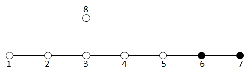
Figure 1: The Dynkin diagram of $E_{8}$. The Dynkin node labelled $i$ corresponds to the exceptional divisor $D_{i}$. The solid nodes are the ones we break by vertical flux, while we preserve a linear combination of their corresponding Cartan generators. The unbroken nodes form the Dynkin diagram of $E_{6}$.

$$\Theta_{1\alpha}=\Theta_{2\alpha}=\Theta_{3\alpha}=\Theta_{4\alpha}=\Theta_{5\alpha}=\Theta_{8\alpha}=a\Theta_{6\alpha}+b\Theta_{7\alpha}=0\,,$$ (42)

where $\alpha$ stands for $S=D^{0}$ and $F=D^{14}$, and $a,b$ are coprime integers. We further require that there is no $E_{8}$ root with the sixth and seventh components along $(a,b)$. Now the above flux constraints are solved by

$$(\phi_{1S},\phi_{2S},\phi_{3S},\phi_{4S},\phi_{5S},\phi_{6S},\phi_{8S})=(2,4,6,5,4,3,3)(a-2b)n_{S}\,,$$

$$\phi_{7S}=(2a-3b)n_{S}\,,$$ (43)

and similarly for $\phi_{iF}$. Since $(a-2b)$ and $(2a-3b)$ are also coprime, $n_{S},n_{F}$ must be integers. Primitivity still requires $n_{S},n_{F}$ to have opposite signs, and we choose $(n_{S},n_{F})=(\pm 1,\mp 1)$ to minimize the tadpole as before. Then Eq. (4) becomes

$$a^{2}-3ab+3b^{2}\leq 37926\,.$$ (44)

Note the similarity to Eq. (36).

We now look at the matter spectrum. The adjoint $\mathbf{248}$ of $E_{8}$ breaks into $E_{6}$ fundamentals $\mathbf{27}$ (and their conjugate) and singlets that are charged under the $\mathrm{U}(1)$. To be precise, the charged representations are

$$\mathbf{27}_{a},\,\mathbf{27}_{a-3b},\,\mathbf{27}_{-2a+3b},\,\mathbf{1}_{3b},\,\mathbf{1}_{3a-3b},\,\mathbf{1}_{3a-6b}\,,$$ (45)

and their conjugates. Similar to the example in Section 4.2, the flux induces no chiral spectrum and the above representations belong to vector-like matter only. The maximum possible charge can be obtained by maximizing the charge of one of the singlets while satisfying Eq. (44). For example, $(a,b)=(2,-111)$ gives maximum $3a-6b=672$ and the charged representations are

$$\mathbf{27}_{2},\,\mathbf{27}_{335},\,\mathbf{27}_{-337},\,\mathbf{1}_{-333},\,\mathbf{1}_{339},\,\mathbf{1}_{672}\,,$$ (46)

and their conjugates. Therefore, we have reached the result $q_{\mathrm{max}}=672$ for $\mathrm{U}(1)$ coupled to $E_{6}$. Note that, as discussed above, the charge is 672 by the definition we are using here where all $\mathrm{U}(1)$ charges are integers, while the spectrum is invariant under the $\mathbb{Z}_{3}$ center of the gauge group. Therefore, it is also natural to normalize the charges with units of $1/3$, in which units the maximum charge would become $q_{\mathrm{max}}=224$. One should thus be careful when interpreting the result in this Section, while the same ambiguity does not occur in Section 4.

It is worth emphasizing again that these models with large $\mathrm{U}(1)$ charges require very non-generic flux configurations, and small $\mathrm{U}(1)$ charges are exponentially preferred in the landscape (assuming a measure where all flux configurations satisfying the tadpole constraint are equally weighted). Heuristically, if one collects all the $\mathrm{U}(1)$ charges of massless states across the landscape, one may expect a distribution that peaks near $q=0$ and decays as $q$ grows Andriolo:2019gcb . This matches the expectation from phenomenology where the $\mathrm{U}(1)$ charges are always small.

We see that no matter how large the charges are, some Yukawa couplings such as $\mathbf{27}^{3}$ in the above models are allowed to be possible from the structure of the unbroken gauge group, while some other couplings are indeed forbidden by the inclusion of exotic $\mathrm{U}(1)$ charges. The above breaking can be straightforwardly generalized to conventional grand unified theories such as $E_{6}\rightarrow\mathrm{SU}(5)\times\mathrm{U}(1)$. Therefore, vertical flux breaking can be useful in phenomenological model building, in which the $\mathrm{U}(1)$ extension may naturally explain issues like proton decay Marsano:2009wr ; Grimm:2010ez . In particular, such constructions can be easily incorporated into the recently proposed natural construction of Standard Model-like structure in F-theory Li:2021eyn ; LiFluxbreaking , as vertical flux breaking is used in both contexts.

6 Conclusion

In this paper, we have studied $\mathrm{U}(1)$ charged massless fields in string theory. While the completeness hypothesis Polchinski:1998rr ; Banks:2010zn ; Harlow:2018tng suggests that states should exist with all possible charges under a U(1) gauge field, in general massless or light fields have small charges. Even in 6D, the upper bound on possible $\mathrm{U}(1)$ charges $q$ for massless fields is not completely understood, with very few explicit string theory constructions of $\mathrm{U}(1)$ models available, and in 4D the question is addressed very little in the literature. Using the formalism of vertical flux breaking, we have efficiently constructed 4D F-theory models containing $\mathrm{U}(1)$ charges for light fields that can be as large as $q=657$, and massless chiral fields with charges that can be at least as large as $q=465$. The string theory construction is fully explicit, using fourfolds with large Euler characteristics in the KS database and exotic flux background. While a rigorous proof is far from complete, we have some reasons to believe that our result gives a plausible upper bound for $\mathrm{U}(1)$ charges in the 4D F-theory landscape, when the $\mathrm{U}(1)$ is decoupled. We have found that the $\mathrm{U}(1)$ charges can become slightly larger when the $\mathrm{U}(1)$ factor is coupled to other gauge groups, although we expect a similar upper bound when for properly normalized charges.

It is worth emphasizing that the Stückelberg mechanism is also available in, for example, type IIB string theory (see e.g. Cvetic:2012xn and the references therein), and one can construct similar $\mathrm{U}(1)$ models in such a perturbative setup. The nonperturbative nature of F-theory, however, allows us to explore a much wider range of compactifications, in particular those containing exceptional gauge groups as in our examples. As a result, F-theory opens up new corners in the string landscape by raising the $\mathrm{U}(1)$ charges that can be explicitly constructed to a much higher value. It remains interesting to compare the upper limits from both F-theory and perturbative string theories.

These results lead in a number of interesting directions. First, as described in Section 1, this class of constructions may give new insights in the context of the Swampland program, as it greatly expands the view on which $\mathrm{U}(1)$ charged massless fields in the low-energy theory can be consistently coupled to gravity. It would be interesting to understand better how these 4D constructions of theories with light fields having large U(1) charges fit with the related 6D analyses of automatic enhancement and of massless charge sufficiency and the completeness hypothesis Raghuram:2020vxm ; Cvetic:2021vsw ; Morrison:2021wuv . More generally, we have found that the formalism of vertical flux breaking leads to large classes of new F-theory models ranging from exotic $\mathrm{U}(1)$ charges to natural Standard Model-like constructions. At the same time, the large charges we have found here are expected to be exponentially rare in any natural measure on the landscape, and this work motivates a more careful study of the impact of the distribution of fluxes on the structure of the gauge group and matter content. While this approach using flux breaking is certainly not completely new in the literature, it has not been fully utilized until now. We hope that this formalism will lead to many more exciting results in F-theory constructions of 4D supergravity models. Finally, this perspective offers new ways of thinking about $\mathrm{U}(1)$ extensions in the Standard Model or grand unified theories. As shown in Section 5, the $\mathrm{U}(1)$ charges we get, albeit exotic, are still potentially relevant to particle phenomenology. It is interesting that the possible appearance of such charges is supported from the UV perspective by explicit string theory constructions.

We hope that future work will lead to a solidification of the arguments for the upper bound on $q$, and the application of this construction of exotic $\mathrm{U}(1)$ charges to broader setups as mentioned in the previous paragraphs.

Appendix A Various descriptions of the geometry

In this Appendix, we compare two descriptions of the geometry in Section 4.1, and show that they are equivalent. One description is a generic elliptic fibration over a given threefold base, and another one is the anticanonical hypersurface in a 5D (singular) weighted projective space.

Let us provide more details on the elliptic fibration. Since the elliptic curve is the CY hypersurface in weighted projective space $\mathbb{P}^{2,3,1}$, the elliptic fibration on a toric base can also be written as the CY hypersurface in a 5D toric ambient space. The toric ambient space is a $\mathbb{P}^{2,3,1}$ fibration over the base, given by the following toric rays:

$$(w_{i},-2,-3)\,,\quad(0,0,0,1,0)\,,\quad(0,0,0,0,1)\,.$$ (47)

The resulting fivefold is singular due to the presence of rigid gauge groups. Those singularities on gauge divisors can be resolved by adding “tops” into the toric fan Candelas:1996su . We do not describe the details here, but one can show that after adding all the tops from Eq. (31), the convex hull of the toric fan is a reflexive polytope with vertices

$$\left(0,0,1,-2,-3\right)\,,\quad\left(-1,-12,0,-2,-3\right)\,,\quad\left(0,1,0,-2,-3\right)\,,$$

$$\left(0,0,0,1,0\right)\,,\quad\left(0,0,0,0,1\right)\,,\quad\left(80,468,-1,-2,-3\right)\,,\quad\left(42,246,0,-2,-3\right)\,.$$ (48)

Notice again that $(80,468)=4v_{19}$ and $(42,246)=6v_{15}$.

Now we perform the following $\mathrm{SL}(5)$ transformation on the vertices:

$$\left(\begin{array}[]{ccccc}0&0&1&0&0\\ -1&0&0&0&0\\ -12&1&0&0&0\\ -26&2&2&1&0\\ -39&3&3&0&1\end{array}\right)\cdot\left(\begin{array}[]{ccccccc}0&-1&0&0&0&80&42\\ 0&-12&1&0&0&468&246\\ 1&0&0&0&0&-1&0\\ -2&-2&-2&1&0&-2&-2\\ -3&-3&-3&0&1&-3&-3\end{array}\right)=\left(\begin{array}[]{ccccccc}1&0&0&0&0&-1&0\\ 0&1&0&0&0&-80&-42\\ 0&0&1&0&0&-492&-258\\ 0&0&0&1&0&-1148&-602\\ 0&0&0&0&1&-1722&-903\end{array}\right)\,.$$ (49)

The geometry described by the polytope should be $\mathrm{SL}(5)$ invariant. On the right hand side, the first six columns are precisely the toric rays of $\mathbb{P}^{1,80,492,1148,1722}$ mentioned in Section 4.1, and the last column represents an exceptional divisor resulting from resolving the singularity in this weighted projective space. These data match those in the KS database. Hence we have proved the equivalence between these two descriptions of the geometry.

References

- (1) M. B. Green and J. H. Schwarz, Anomaly Cancellation in Supersymmetric D=10 Gauge Theory and Superstring Theory, Phys. Lett. B 149 (1984) 117.
- (2) D. J. Gross, J. A. Harvey, E. J. Martinec and R. Rohm, The Heterotic String, Phys. Rev. Lett. 54 (1985) 502.
- (3) A. Adams, O. DeWolfe and W. Taylor, String universality in ten dimensions, Phys. Rev. Lett. 105 (2010) 071601 [1006.1352].
- (4) H.-C. Kim, G. Shiu and C. Vafa, Branes and the Swampland, Phys. Rev. D 100 (2019) 066006 [1905.08261].
- (5) C. Vafa, The String landscape and the swampland, [hep-th/0509212].
- (6) H. Ooguri and C. Vafa, On the Geometry of the String Landscape and the Swampland, Nucl. Phys. B766 (2007) 21 [hep-th/0605264].
- (7) M. van Beest, J. Calderón-Infante, D. Mirfendereski and I. Valenzuela, Lectures on the Swampland Program in String Compactifications, 2102.01111.
- (8) P. Candelas, E. Perevalov and G. Rajesh, Toric geometry and enhanced gauge symmetry of F theory / heterotic vacua, Nucl. Phys. B 507 (1997) 445 [hep-th/9704097].
- (9) P. S. Aspinwall and D. R. Morrison, Point - like instantons on K3 orbifolds, Nucl. Phys. B 503 (1997) 533 [hep-th/9705104].
- (10) D. R. Morrison and W. Taylor, Toric bases for 6D F-theory models, Fortsch. Phys. 60 (2012) 1187 [1204.0283].
- (11) Y.-N. Wang, On the Elliptic Calabi-Yau Fourfold with Maximal , JHEP 05 (2020) 043 [2001.07258].
- (12) K. R. Dienes and J. March-Russell, Realizing higher level gauge symmetries in string theory: New embeddings for string GUTs, Nucl. Phys. B 479 (1996) 113 [hep-th/9604112].
- (13) D. Klevers, D. R. Morrison, N. Raghuram and W. Taylor, Exotic matter on singular divisors in F-theory, 1706.08194.
- (14) M. Cvetič, J. J. Heckman and L. Lin, Towards Exotic Matter and Discrete Non-Abelian Symmetries in F-theory, JHEP 11 (2018) 001 [1806.10594].
- (15) C. Vafa, Evidence for F theory, Nucl. Phys. B469 (1996) 403 [hep-th/9602022].
- (16) D. R. Morrison and C. Vafa, Compactifications of F theory on Calabi–Yau threefolds — I, Nucl. Phys. B473 (1996) 74 [hep-th/9602114].
- (17) D. R. Morrison and C. Vafa, Compactifications of F theory on Calabi–Yau threefolds — II, Nucl. Phys. B476 (1996) 437 [hep-th/9603161].
- (18) J. Polchinski, String theory. Vol. 2: Superstring theory and beyond, Cambridge Monographs on Mathematical Physics. Cambridge University Press, 12, 2007, 10.1017/CBO9780511618123.
- (19) T. Banks and N. Seiberg, Symmetries and Strings in Field Theory and Gravity, Phys. Rev. D 83 (2011) 084019 [1011.5120].
- (20) D. Harlow and H. Ooguri, Symmetries in quantum field theory and quantum gravity, Commun. Math. Phys. 383 (2021) 1669 [1810.05338].
- (21) T. Weigand, TASI Lectures on F-theory, [1806.01854].
- (22) D. R. Morrison and W. Taylor, Charge completeness and the massless charge lattice in F-theory models of supergravity, JHEP 12 (2021) 040 [2108.02309].
- (23) K. Kodaira, On compact analytic surfaces: Ii, Annals of Mathematics 77 (1963) 563.
- (24) A. Néron, Modèles minimaux des variétés abéliennes sur les corps locaux et globaux, Publications Mathématiques de l’IHÉS 21 (1964) 5.
- (25) M. Bershadsky, K. A. Intriligator, S. Kachru, D. R. Morrison, V. Sadov and C. Vafa, Geometric singularities and enhanced gauge symmetries, Nucl. Phys. B481 (1996) 215 [hep-th/9605200].
- (26) S. H. Katz and C. Vafa, Matter from geometry, Nucl. Phys. B497 (1997) 146 [hep-th/9606086].
- (27) P. S. Aspinwall and D. R. Morrison, Nonsimply connected gauge groups and rational points on elliptic curves, JHEP 07 (1998) 012 [hep-th/9805206].
- (28) P. S. Aspinwall, S. H. Katz and D. R. Morrison, Lie groups, Calabi-Yau threefolds, and F theory, Adv. Theor. Math. Phys. 4 (2000) 95 [hep-th/0002012].
- (29) T. W. Grimm and T. Weigand, On Abelian Gauge Symmetries and Proton Decay in Global F-theory GUTs, Phys. Rev. D 82 (2010) 086009 [1006.0226].
- (30) D. R. Morrison and D. S. Park, F-Theory and the Mordell–Weil Group of Elliptically-Fibered Calabi–Yau Threefolds, JHEP 10 (2012) 128 [1208.2695].
- (31) D. Klevers, D. K. Mayorga Pena, P.-K. Oehlmann, H. Piragua and J. Reuter, F-Theory on all Toric Hypersurface Fibrations and its Higgs Branches, JHEP 01 (2015) 142 [1408.4808].
- (32) N. Raghuram, Abelian F-theory Models with Charge-3 and Charge-4 Matter, JHEP 05 (2018) 050 [1711.03210].
- (33) J. Knapp, E. Scheidegger and T. Schimannek, On genus one fibered Calabi-Yau threefolds with 5-sections, 2107.05647.
- (34) F. M. Cianci, D. K. Mayorga Peña and R. Valandro, High U(1) charges in type IIB models and their F-theory lift, JHEP 04 (2019) 012 [1811.11777].
- (35) A. Collinucci, M. Fazzi, D. R. Morrison and R. Valandro, High electric charges in M-theory from quiver varieties, JHEP 11 (2019) 111 [1906.02202].
- (36) N. Raghuram and W. Taylor, Large U(1) charges in F-theory, JHEP 10 (2018) 182 [1809.01666].
- (37) N. Raghuram and A. P. Turner, Orders of vanishing and U(1) charges in F-theory, JHEP 03 (2022) 051 [2110.10159].
- (38) W. Taylor and A. P. Turner, An infinite swampland of U(1) charge spectra in 6D supergravity theories, JHEP 06 (2018) 010 [1803.04447].
- (39) N. Raghuram, W. Taylor and A. P. Turner, Automatic enhancement in 6D supergravity and F-theory models, JHEP 07 (2021) 048 [2012.01437].
- (40) M. Cvetic, L. Lin and A. P. Turner, Flavor symmetries and automatic enhancement in the 6D supergravity swampland, Phys. Rev. D 105 (2022) 046005 [2110.00008].
- (41) S. Y. Li and W. Taylor, Gauge symmetry breaking with fluxes and natural Standard Model structure from exceptional GUTs in F-theory, 2207.14319.
- (42) E. Witten, On flux quantization in M theory and the effective action, J. Geom. Phys. 22 (1997) 1 [hep-th/9609122].
- (43) S. Sethi, C. Vafa and E. Witten, Constraints on low dimensional string compactifications, Nucl. Phys. B 480 (1996) 213 [hep-th/9606122].
- (44) M. Kreuzer and H. Skarke, Calabi-Yau four folds and toric fibrations, J. Geom. Phys. 26 (1998) 272 [hep-th/9701175].
- (45) F. Schöller and H. Skarke, All Weight Systems for Calabi–Yau Fourfolds from Reflexive Polyhedra, Commun. Math. Phys. 372 (2019) 657 [1808.02422].
- (46) T. Shioda, On elliptic modular surfaces, J. Math. Soc. Japan 24 (1972) 20.
- (47) R. Wazir, Arithmetic on elliptic threefolds, Compositio Mathematica 140 (2004) 567–580 [math/0112259].
- (48) P. Jefferson, W. Taylor and A. P. Turner, Chiral matter multiplicities and resolution-independent structure in 4D F-theory models, 2108.07810.
- (49) K. Becker and M. Becker, M theory on eight manifolds, Nucl. Phys. B 477 (1996) 155 [hep-th/9605053].
- (50) S. Gukov, C. Vafa and E. Witten, CFT’s from Calabi-Yau four folds, Nucl. Phys. B 584 (2000) 69 [hep-th/9906070].
- (51) A. P. Braun and T. Watari, The Vertical, the Horizontal and the Rest: anatomy of the middle cohomology of Calabi-Yau fourfolds and F-theory applications, JHEP 01 (2015) 047 [1408.6167].
- (52) T. W. Grimm and H. Hayashi, F-theory fluxes, Chirality and Chern-Simons theories, JHEP 03 (2012) 027 [1111.1232].
- (53) T. W. Grimm and R. Savelli, Gravitational Instantons and Fluxes from M/F-theory on Calabi-Yau fourfolds, Phys. Rev. D 85 (2012) 026003 [1109.3191].
- (54) K. Dasgupta, G. Rajesh and S. Sethi, M theory, orientifolds and G - flux, JHEP 08 (1999) 023 [hep-th/9908088].
- (55) C. Beasley, J. J. Heckman and C. Vafa, GUTs and Exceptional Branes in F-theory - I, JHEP 01 (2009) 058 [0802.3391].
- (56) M. Buican, D. Malyshev, D. R. Morrison, H. Verlinde and M. Wijnholt, D-branes at Singularities, Compactification, and Hypercharge, JHEP 01 (2007) 107 [hep-th/0610007].
- (57) C. Beasley, J. J. Heckman and C. Vafa, GUTs and Exceptional Branes in F-theory - II: Experimental Predictions, JHEP 01 (2009) 059 [0806.0102].
- (58) T. W. Grimm, The N=1 effective action of F-theory compactifications, Nucl. Phys. B 845 (2011) 48 [1008.4133].
- (59) T. W. Grimm, M. Kerstan, E. Palti and T. Weigand, Massive Abelian Gauge Symmetries and Fluxes in F-theory, JHEP 12 (2011) 004 [1107.3842].
- (60) A. Braun, A. Collinucci and R. Valandro, G-flux in f-theory and algebraic cycles, Nuclear Physics B 856 (2012) 129–179 [1107.5337].
- (61) J. Marsano and S. Schäfer-Nameki, Yukawas, g-flux, and spectral covers from resolved calabi-yau’s, Journal of High Energy Physics 2011 (2011) [1108.1794].
- (62) S. Krause, C. Mayrhofer and T. Weigand, G4-flux, chiral matter and singularity resolution in f-theory compactifications, Nuclear Physics B 858 (2012) 1 [1109.3454].
- (63) W. Taylor and Y.-N. Wang, The F-theory geometry with most flux vacua, JHEP 12 (2015) 164 [1511.03209].
- (64) D. R. Morrison and W. Taylor, Classifying bases for 6D F-theory models, Central Eur. J. Phys. 10 (2012) 1072 [1201.1943].
- (65) D. R. Morrison and W. Taylor, Non-Higgsable clusters for 4D F-theory models, JHEP 05 (2015) 080 [1412.6112].
- (66) J. J. Heckman, D. R. Morrison and C. Vafa, On the Classification of 6D SCFTs and Generalized ADE Orbifolds, JHEP 05 (2014) 028 [1312.5746].
- (67) M. Del Zotto, J. J. Heckman, A. Tomasiello and C. Vafa, 6d Conformal Matter, JHEP 02 (2015) 054 [1407.6359].
- (68) F. Apruzzi, J. J. Heckman, D. R. Morrison and L. Tizzano, 4D Gauge Theories with Conformal Matter, JHEP 09 (2018) 088 [1803.00582].
- (69) L. B. Anderson, J. Gray and P.-K. Oehlmann, F-Theory on Quotients of Elliptic Calabi-Yau Threefolds, JHEP 12 (2019) 131 [1906.11955].
- (70) V. Braun and D. R. Morrison, F-theory on Genus-One Fibrations, JHEP 08 (2014) 132 [1401.7844].
- (71) D. R. Morrison and W. Taylor, Sections, multisections, and U(1) fields in F-theory, 1404.1527.
- (72) J. Gray, A. S. Haupt and A. Lukas, Topological Invariants and Fibration Structure of Complete Intersection Calabi-Yau Four-Folds, JHEP 09 (2014) 093 [1405.2073].
- (73) M. Gross, A finiteness theorem for elliptic Calabi–Yau threefolds, Duke Math. Jour. 15 (2011) 325.
- (74) A. Grassi, On minimal models of elliptic threefolds., Mathematische Annalen 290 (1991) 287.
- (75) W. Taylor, On the Hodge structure of elliptically fibered Calabi-Yau threefolds, JHEP 08 (2012) 032 [1205.0952].
- (76) W. Taylor and Y.-N. Wang, Non-toric bases for elliptic Calabi–Yau threefolds and 6D F-theory vacua, Adv. Theor. Math. Phys. 21 (2017) 1063 [1504.07689].
- (77) M. Kreuzer and H. Skarke, Complete classification of reflexive polyhedra in four-dimensions, Adv. Theor. Math. Phys. 4 (2000) 1209 [hep-th/0002240].
- (78) A. Klemm, B. Lian, S.-S. Roan and S.-T. Yau, Calabi-yau four-folds for m- and f-theory compactifications, Nuclear Physics B 518 (1998) 515–574.
- (79) J. Halverson and W. Taylor, -bundle bases and the prevalence of non-Higgsable structure in 4D F-theory models, JHEP 09 (2015) 086 [1506.03204].
- (80) W. Taylor and Y.-N. Wang, A Monte Carlo exploration of threefold base geometries for 4d F-theory vacua, JHEP 01 (2016) 137 [1510.04978].
- (81) J. Halverson, C. Long and B. Sung, Algorithmic universality in F-theory compactifications, Phys. Rev. D96 (2017) 126006 [1706.02299].
- (82) W. Taylor and Y.-N. Wang, Scanning the skeleton of the 4D F-theory landscape, JHEP 01 (2018) 111 [1710.11235].
- (83) A. P. Braun, A. Collinucci and R. Valandro, Hypercharge flux in F-theory and the stable Sen limit, JHEP 07 (2014) 121 [1402.4096].
- (84) G. Di Cerbo and R. Svaldi, Birational boundedness of low-dimensional elliptic calabi–yau varieties with a section, Compositio Mathematica 157 (2021) 1766.
- (85) C. Lawrie, S. Schafer-Nameki and J.-M. Wong, F-theory and All Things Rational: Surveying U(1) Symmetries with Rational Sections, JHEP 09 (2015) 144 [1504.05593].
- (86) T. W. Grimm, A. Kapfer and D. Klevers, The Arithmetic of Elliptic Fibrations in Gauge Theories on a Circle, JHEP 06 (2016) 112 [1510.04281].
- (87) M. Cvetič and L. Lin, The Global Gauge Group Structure of F-theory Compactification with s, JHEP 01 (2018) 157 [1706.08521].
- (88) W. Taylor and A. P. Turner, Generic matter representations in 6D supergravity theories, JHEP 05 (2019) 081 [1901.02012].
- (89) W. Taylor and A. P. Turner, Generic construction of the Standard Model gauge group and matter representations in F-theory, 1906.11092.
- (90) S. Andriolo, S. Y. Li and S. H. H. Tye, String Landscape and Fermion Masses, Phys. Rev. D 101 (2020) 066005 [1902.06608].
- (91) J. Marsano, N. Saulina and S. Schafer-Nameki, Compact F-theory GUTs with U(1) (PQ), JHEP 04 (2010) 095 [0912.0272].
- (92) S. Y. Li and W. Taylor, Natural F-theory constructions of Standard Model structure from flux breaking, 2112.03947.
- (93) P. Candelas and A. Font, Duality between the webs of heterotic and type II vacua, Nucl. Phys. B 511 (1998) 295 [hep-th/9603170].