A Low Latency Adaptive Coding Spike Framework for Deep Reinforcement Learning

Abstract

In recent years, spiking neural networks (SNNs) have been used in reinforcement learning (RL) due to their low power consumption and event-driven features. However, spiking reinforcement learning (SRL), which suffers from fixed coding methods, still faces the problems of high latency and poor versatility. In this paper, we use learnable matrix multiplication to encode and decode spikes, improving the flexibility of the coders and thus reducing latency. Meanwhile, we train the SNNs using the direct training method and use two different structures for online and offline RL algorithms, which gives our model a wider range of applications. Extensive experiments have revealed that our method achieves optimal performance with ultra-low latency (as low as 0.8% of other SRL methods) and excellent energy efficiency (up to 5X the DNNs) in different algorithms and different environments.

1 Introduction

Deep learning has had a significant impact on many areas of machine learning, including reinforcement learning (RL). The combination of deep learning algorithms and RL has led to the development of a new field called deep reinforcement learning (DRL) Arulkumaran et al. (2017), which has achieved impressive results in a variety of RL tasks, including some that have reached or even surpassed human-level performance Mnih et al. (2015); Hu et al. (2021); Silver et al. (2016). However, DRL using deep neural networks (DNNs) requires a significant amount of resources, which may not always be available. For example, in the case of mobile robots, the processing system needs to be power-efficient and have low latency (inference time) Niroui et al. (2019); Lahijanian et al. (2018). As a result, researchers are actively exploring the use of alternative networks for DRL that are more energy-efficient and have lower latency.

Inspired by neurobiology, spiking neural networks (SNNs) use differential dynamics equations and spike information encoding methods to build computing node models in neural networks Maass (1997). Compared with DNNs, SNNs are closer to biological neural networks and could greatly reduce energy consumption with neuromorphic hardware. Therefore, SNNs are well suited as a low-power alternative to DNNs in DRL. But there is still relatively little attempt at using SNNs in RL to achieve high-dimensional control with low latency (inference time steps) and energy consumption.

The existing spiking reinforcement learning (SRL) methods are mainly divided into two categories Neftci and Averbeck (2019). First, guided by revealing reward mechanisms in the brain, several works Yuan et al. (2019); Bing et al. (2018); Frémaux et al. (2013) train spiking neurons with reward-based local learning rules. These local learning methods can only be applied for simple control with shallow SNNs. Second, oriented toward better performance, replacing DNNs in DRL with SNNs can also implement SRL. Since SNNs usually use the firing rate as the equivalent activation value Li et al. (2021), which is a discrete value between 0 and 1, it is hard to represent the value function of RL, which does not have a certain range in training. To avoid using discrete spikes to calculate the value function, this type of method is subdivided into three types. Tan Tan et al. (2021) and Patel Patel et al. (2019) use the SNN conversion method to convert the Deep Q-Networks (DQN) Mnih et al. (2015) into SNNs. Zhang Zhang et al. (2022) and Tang Tang et al. (2020) use the hybrid framework, which uses DNNs for value function estimation and SNNs for execution. Chen Chen et al. (2022) and Liu Liu et al. (2022) use surrogate gradients to train SNNs directly and fixed spike coders to estimate the value function.

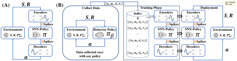
Figure 1: Online and offline SRL frameworks. Environments generally contain elements such as states ($S$), rewards ($R$), and state transition probabilities ($P_{ss^{\prime}}^{a}$). The state ($S$) is transmitted to the SNNs through the encoders. Action ($a$) and value functions are expressed by the decoders. The environment accepts the action ($a$) and gives the next state ($S^{\prime}$) based on the transition probability ($P_{ss^{\prime}}^{a}$). (A) In online SRL, the SNN-based policy $\pi$ interacts directly with the environment. (B) In offline SRL, the SNN-based policy interacts with a dataset $\mathcal{D}$ which collected by the behavior policy $\pi_{\beta}$. The behavior policy are usually developed by experienced humans or well-trained agent.

However, these methods all have their shortcomings. Conversion methods have low energy efficiency and high latency, while the hybrid framework loses the potential biological plausibility of SNNs and limits the application of different types of RL algorithms. Although the directly trained SNNs have high energy efficiency and low latency, they are hard to estimate for continuous-valued functions using fixed coders. They have to find a trade-off between latency and accuracy Li et al. (2022). In addition, these SRL methods have a narrow range of applications because they are all limited to a specific online RL algorithm (DQN, TD3 Fujimoto et al. (2018), and DDPG Lillicrap et al. (2016)).

To overcome these shortcomings, we propose an adaptive coding method to compress or extend information in the temporal dimension through learnable matrix multiplication. This learnable code offers increased flexibility over fixed coding, allowing for better results with lower latency. Unlike sequence-to-sequence coding in Shrestha and Orchard (2018) and Hagenaars et al. (2021), our proposed adaptive coder implements value-sequence coding. Moreover, our coders do not require a label signal and can automatically select the optimal form according to different tasks.

At the same time, in order to expand the scope of application, we design structures for online and offline SRL algorithms, respectively. Figure 1A shows the flow of the online algorithm, where the state and reward of the environment are directly interacted with the spiking agent after passing through the encoder. SNN calculates the value function and outputs it in the form of spikes, which are converted into real values by decoders. Finally, the action selection is made according to the value function. Offline algorithms are more complex (Figure 1B). It begins by collecting data through behavioral policies that interact with the environment. Then, the spiking agent interacts with the collected data and learns through the same process as online algorithms. We named the proposed SRL model adaptive coding spike framework (ACSF). The main contributions of this paper can be summarized as follows:

• We propose an adaptive coding spike framework for SRL that uses adaptive coders to represent states and estimate value functions. This framework reduces the latency of existing methods effectively while maintaining optimal performance.

• To our best knowledge, the ACSF is the first complete, directly trained SRL framework. It supports both online and offline RL algorithms, expanding the application range of SRL.

• For the RL scale, ACSF provides a low-power inference scheme for RL algorithms (up to 5X energy efficient). This provides potential assistance for mobile robot control using RL algorithms.

• From the experimental results, compared with conversion and other directly trained methods, ACSF has better versatility and lower latency ($T=4$). At the same time, it achieves the best performance in all conditions.

2 Related Works

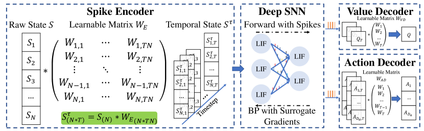
Figure 2: The overall structure and workflow of the ACSF. The encoder transforms the raw state $S$ into the temporal state $S^{\tau}$, which is then fed into SNNs. The output spike trains generated by SNNs are decoded into values or actions by different decoders. Both the spike encoder and the decoder use learnable matrix multiplication to expand or compress inputs in the time dimension. Deep SNNs are trained directly using surrogate gradients.

2.1 Reward-based Local Learning

To explore the reward mechanism in the brain, applying reward-based training rules to the local learning of spiking neurons Yuan et al. (2019); Bing et al. (2018); Frémaux et al. (2013); Legenstein et al. (2008) was the mainstream approach for early SRL. However, they have the common problem that they are limited to shallow SNNs and are hard to apply to complex tasks. E-prop Bellec et al. (2020) successfully advances SRL to complex tasks with good performance. However, it needs to tune a lot of hyperparameters, making it difficult to apply to different RL tasks.

2.2 Convert DNNs to SNNs for RL

The conversion algorithms map the DNNs to the SNNs by matching the firing rate and activation values. It is a commonly used method for obtaining high-performance SNNs. Several works Tan et al. (2021); Patel et al. (2019) obtain Deep Spiking Q-Networks (DSQN) using conversion methods. To ensure the accuracy of mapping, those methods often have high latency (about 500 time steps) and cannot outperform the source DQNs.

2.3 Hybrid Framework of SNNs and DNNs

In RL, some algorithms use the actor-critic architecture Sutton et al. (1999), where value function estimation and action selection are implemented by critic and actor networks, respectively. Some works Zhang et al. (2022); Tang et al. (2020) use deep critic networks and spiking actor networks to implement SRL. These methods can be applied to complex tasks with lower latency, but they only work for actor-critic structures, and they rely on DNNs, which makes them difficult to fully apply to neuromorphic chips.

2.4 Directly Trained SNNs for RL

Surrogate gradient methods introduce backpropagation (BP) into SNNs successfully and make it easy to train deep SNNs directly. Recently, a few papers Chen et al. (2022); Liu et al. (2022) have used directly trained SNNs and fixed coders to construct DSQN. Although these methods have high energy efficiency, they do not form a complete framework and have a poor trade-off between accuracy and latency. In addition, their applications are also limited to discrete action-space environments.

3 Methods

In this section, we first introduce the DRL algorithms and the spiking neuron model. Then, we describe the adaptive coding method in detail. Finally, we derive the gradient of the direct training method. The overall architecture of ACSF is shown in Figure 2.

3.1 DRL Algorithms

In this section, we will introduce different baseline algorithms (DQN, DDPG, BCQ and behavioral cloning) used in ACSF. Due to space limitations, we only show the final loss functions. Please refer to the supplementary materials for more details. Assume the agent’s current environment sampling result is state $s$, action $a$, reward $r$ and next state $s^{\prime}$. Mark the reward discount factor as $\gamma$.

3.1.1 DQN

DQN is a typical RL algorithm, and it only needs to learn the value function ($q$-values). Its loss function Girshick (2015) is:

$$\begin{split}&smooth_{L_{1}}(x)=\left\{\begin{array}[]{ll}0.5x^{2}&if|x|<1\\ |x|-0.5&otherwise\end{array}\right.\\ &\mathcal{L}_{Q}=smooth_{L_{1}}[r+\gamma\max_{a^{\prime}}Q_{\theta_{2}}(s^{\prime},a^{\prime})-Q_{\theta_{1}}(s,a)]\end{split}$$ (1)

where $Q_{\theta_{1}}$ and $Q_{\theta_{2}}$ is the current and target $q$-networks, respectively.

3.1.2 DDPG

DDPG is based on AC architecture, including actor networks that select actions and critic networks that calculate value functions. The loss functions of the actor and critic networks are:

$$\begin{split}\mathcal{L}_{A}&=-\frac{1}{N}\sum_{j=1}^{N}Q_{\theta_{1}}(s,A_{\phi_{1}}(s))\\ \mathcal{L}_{Q}&=\frac{1}{N}\sum_{j=1}^{N}[r+\gamma Q_{\theta_{2}}(s^{\prime},A_{\phi_{2}}(s^{\prime}))-Q_{\theta_{1}}(s,a)]^{2}\end{split}$$ (2)

where $Q_{\theta_{1}}$ and $Q_{\theta_{2}}$ are current and target critic networks; $A_{\phi_{1}}$ and $A_{\phi_{2}}$ are current and target actor networks. $N$ is the batch size.

3.1.3 BCQ

BCQ is an offline RL algorithm. In addition to training double critic networks $Q^{1}_{\theta_{1}},Q^{2}_{\theta_{1}}$, target critic networks $Q^{1}_{\theta_{2}},Q^{2}_{\theta_{2}}$, current perturbation network $\xi_{\delta_{1}}$ and target perturbation network $\xi_{\delta_{2}}$, we also need to train a variational auto-encoder (VAE) Kingma and Welling (2014) $G_{\omega}=\left\{{E_{\omega_{1}},D_{\omega_{2}}}\right\}$. Their loss functions can be written as follows Fujimoto et al. (2019):

$$\begin{split}&\mathcal{L}_{G}=\sum(a-\widetilde{a})^{2}+D_{KL}(\mathcal{N}(\mu,\sigma)||\mathcal{N}(0,1))\\ &\mathcal{L}_{Q}=\frac{1}{2}\sum[y-Q^{1}_{\theta_{1}}(s,a)]^{2}+\frac{1}{2}\sum[y-Q^{2}_{\theta_{1}}(s,a)]^{2}\\ &\mathcal{L}_{\xi}=-\sum Q^{1}_{\theta_{1}}(s,a+\xi_{\delta_{1}}(s,a,\Phi)),a\sim G_{\omega}(s)\end{split}$$ (3)

3.1.4 Behavioral Cloning

Behavioral cloning (BC) is an offline imitation learning method used to fit the distribution of buffered data $\mathcal{D}$. We use a multilayer perceptron (MLP) $P_{\kappa}$ in this work. The input of the MLP model is raw states ($s$), and the output is action ($a$). We use the mean squared error (MSE) as the loss function:

$$\begin{split}\mathcal{L}_{P}=\frac{1}{2}\sum_{i=1}^{m}[P_{\kappa}(s)-a]^{2}\end{split}$$ (4)

where $m$ is the dimension of action.

3.2 Iterative LIF Model

In this work, we employ the iterative leaky integrate-and-fire (LIF) neuron model to drive the proposed ACSF due to its biological plausibility and computational tractability. Its dynamics can be described by three processes: charge, discharge, and reset. The corresponding equations are:

$$V^{l}_{t} =\beta\hat{V}^{l}_{t-1}+(1-\beta)W^{l}O^{l-1}_{t} Charge$$ (5)

$$O^{l}_{t} =\Theta(V^{l}_{t}),\ \Theta(x)=\left\{\begin{array}[]{l}1,x\geq\vartheta\\ 0,x<\vartheta\end{array}\right. Discharge$$

$$\hat{V}^{l}_{t} =V_{r}O^{l}_{t}+(1-O^{l}_{t})V^{l}_{t} Reset$$

where the superscript $l$ indicates the $l$-th layer, the subscript $t$ represents the $t$-th time step; $V$ and $\hat{V}$ denote the membrane potential before and after reset respectively; $\beta$ is the decay factor; $O$ is the output spike; $\Theta(\cdot)$ is the firing function; $V_{r}$ is the reset voltage; $\vartheta$ is the firing threshold. The schematic diagram of neuron dynamics is shown in Figure 3.

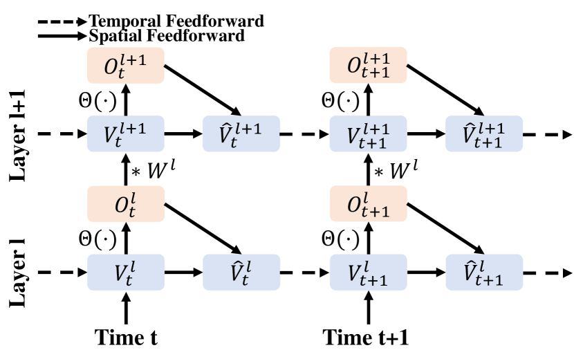
Figure 3: Spatiotemporal dynamics of neurons. The solid arrows and the dotted arrows indicate the directions of spatial and temporal feedforward, respectively. The input signal changes the membrane potential ($V^{l}_{t}$) and fires the output spikes ($O^{l}_{t}$) through the processes of charging, discharging, and resetting.

3.3 Adaptive Coders

As mentioned earlier, existing directly trained SRL methods have limited application and poor trade-offs between performance and latency. The key to solving these problems is to design a common adaptive coder with learnable weights that allows the model to be adapted to different algorithms and environments. In addition, adaptive coding has better characterization capabilities than fixed coding and can achieve better performance with lower latency.

3.3.1 Spike Encoder

There are many fixed encoding methods in SRL, such as rate coding, population coding, and temporal coding. Although these methods have had some success, they are frequently rigid, with strict time step length requirements. To increase flexibility and reduce latency, we encode the raw state $S$ with a learnable matrix $W_{E}$ (Figure 2). We use matrix multiplication to expand $S$ in the temporal dimension by $T$ times, yielding the temporal state $S^{\tau}$. The temporal state $S^{\tau}$ is then fed into the spiking neurons, which produce spike trains $O_{t}$. The encoding strategy at the $t$-th time step can be stated as follows:

$$S^{\tau}=S*W_{E}$$ (6)

$$V_{t}=\beta\hat{V}_{t-1}+(1-\beta)S^{\tau}_{t}$$

$$\hat{V}_{t}=(1-O_{t})V_{t}+V_{r}O_{t}$$

$$O_{t}=\Theta(V_{t})$$

where $S$ and $S^{\tau}$ denote the state and temporal state, respectively; $O_{t}$ is the output spike at the $t$-th time step; $*$ represents the matrix multiplication; and $W_{E}$ is the learnable matrix that can be jointly optimized.

3.3.2 Decoders

The decoding method used in SRL is usually rate decoding. The accuracy of this decoding method is proportional to the length of the time step, so it is difficult to strike a good trade-off between performance and latency. To improve the performance of decoding at low latency, we use an operation similar to adaptive encoding. We multiply the spike trains with a learnable matrix $W_{D}$ to compress them $T$ times in the time dimension:

$$\left\{\begin{aligned} Q&=Q^{\tau}*W_{VD}\\ A&=A^{\tau}*W_{AD}\end{aligned}\right.$$ (7)

where $Q^{\tau}$ and $A^{\tau}$ are output spike trains of the value network and action network, respectively; $W_{VD}$ and $W_{AD}$ are decode matrices of the value decoder and action decoder; and $Q/A$ are the value function and actions selection of RL. Specially, for RL algorithms with non-AC architectures such as DQN, we only decode the $Q$ values.

3.4 Direct Training with Surrogate Gradients

Compared with SNNs obtained using conversion methods, directly trained SNNs tend to have lower latency and higher inference energy efficiency. However, the non-differentiable property of spikes makes directly training SNNs difficult. The surrogate gradient method solves this problem by using alternative activation functions and is widely used to train deep SNNs Wu et al. (2018). We adopt the arctangent function as the surrogate gradient function:

$$\begin{split}\Theta^{\prime}(x)&\triangleq h^{\prime}(x)=\frac{\alpha}{2[1+(\frac{\pi}{2}\alpha x)^{2}]}\end{split}$$ (8)

where $\alpha$ is a hyperparameter that controls the width of the surrogate function.

Suppose the loss function is $\mathcal{L}$, according to Eq. 7 and the chain rule, for the decoding matrix, we have:

$$\left\{\begin{aligned} \frac{\partial\mathcal{L}_{Q}}{\partial W_{VD}}=\frac{\partial\mathcal{L}_{Q}}{\partial Q}\frac{\partial Q}{\partial W_{VD}}=\frac{\partial\mathcal{L}_{Q}}{\partial Q}Q^{\tau}\\ \frac{\partial\mathcal{L}_{A}}{\partial W_{AD}}=\frac{\partial\mathcal{L}_{A}}{\partial A}\frac{\partial A}{\partial W_{AD}}=\frac{\partial\mathcal{L}_{A}}{\partial A}A^{\tau}\end{aligned}\right.$$ (9)

and for the final layer $L$:

$$\frac{\partial\mathcal{L}}{\partial W^{L}}=\left\{\begin{aligned} \frac{\partial\mathcal{L}_{Q}}{\partial Q}\frac{\partial Q}{\partial W^{L}}=\frac{\partial\mathcal{L}_{Q}}{\partial Q}\sum_{t=1}^{T}\frac{\partial Q^{\tau}_{t}}{\partial W^{L}}*W_{VD}\\ \frac{\partial\mathcal{L}_{A}}{\partial A}\frac{\partial A}{\partial W^{L}}=\frac{\partial\mathcal{L}_{A}}{\partial A}\sum_{t=1}^{T}\frac{\partial A^{\tau}_{t}}{\partial W^{L}}*W_{AD}\end{aligned}\right.$$ (10)

where $\frac{\partial\mathcal{L}_{Q}}{\partial Q}$ and $\frac{\partial\mathcal{L}_{A}}{\partial A}$ are defined according to different algorithms; $Q^{\tau}_{t}$ and $A^{\tau}_{t}$ are output spike trains, equal to $O^{L}_{t}$, so we only need to calculate $\frac{\partial O^{L}_{t}}{\partial W^{L}}$:

$$\begin{split}\frac{\partial O^{L}_{t}}{\partial W^{L}}&=\frac{\partial O^{L}_{t}}{\partial V^{L}_{t}}\frac{\partial V^{L}_{t}}{\partial W^{L}}=\frac{\partial\Theta(V^{L}_{t})}{\partial V^{L}_{t}}(1-\beta)O^{l-1}_{t}\\ &=h^{\prime}(V^{L}_{t})(1-\beta)O^{l-1}_{t}\end{split}$$ (11)

and for the hidden layers $l\in\{1,\cdots,L-1\}$, according to Eq. 5:

$$\frac{\partial\mathcal{L}}{\partial W^{l}}=\sum_{t=1}^{T}\frac{\partial\mathcal{L}}{\partial O^{l}_{t}}\frac{\partial O^{l}_{t}}{\partial V^{l}_{t}}\frac{\partial V^{l}_{t}}{\partial W^{l}}$$ (12)

where $T$ is the total time steps.

The first factor in Eq. 12 could be derived as:

$$\begin{split}\frac{\partial\mathcal{L}}{\partial O^{l}_{t}}&=\frac{\partial\mathcal{L}}{\partial O^{l+1}_{t}}\frac{\partial O^{l+1}_{t}}{\partial V^{l+1}_{t}}\frac{\partial V^{l+1}_{t}}{\partial O^{l}_{t}}\\ &=\frac{\partial\mathcal{L}}{\partial O^{l+1}_{t}}h^{\prime}(V^{l+1}_{t})(1-\beta)W^{l+1}\end{split}$$ (13)

The second factor in Eq. 12 could be derived as:

$$\begin{split}\frac{\partial O^{l}_{t}}{\partial V^{l}_{t}}=\frac{\partial\Theta(V^{l}_{t})}{\partial V^{l}_{t}}=h^{\prime}(V^{l}_{t})\end{split}$$ (14)

The third factor in Eq. 12 could be derived as:

$$\begin{split}\frac{\partial V^{l}_{t}}{\partial W^{l}}&=\beta\frac{\partial\hat{V}^{l}_{t-1}}{\partial W^{l}}+(1-\beta)O^{l-1}_{t}\\ \end{split}$$ (15)

where:

$$\begin{split}\frac{\partial\hat{V}^{l}_{t-1}}{\partial W^{l}}&=V_{r}\frac{\partial O^{l}_{t-1}}{\partial W^{l}}+(1-O^{l}_{t-1})\frac{\partial V^{l}_{t-1}}{\partial W^{l}}-V^{l}_{t-1}\frac{\partial O^{l}_{t-1}}{\partial W^{l}}\\ &=(V_{r}-V^{l}_{t-1})h^{\prime}(V^{l}_{t-1})\frac{\partial V^{l}_{t-1}}{\partial W^{l}}+(1-O^{l}_{t-1})\frac{\partial V^{l}_{t-1}}{\partial W^{l}}\\ &=[(V_{r}-V^{l}_{t-1})h^{\prime}(V^{l}_{t-1})+(1-O^{l}_{t-1})]\frac{\partial V^{l}_{t-1}}{\partial W^{l}}\end{split}$$ (16)

Let:

$$\begin{split}\phi_{t}&\triangleq\beta[(V_{r}-V^{l}_{t-1})h^{\prime}(V^{l}_{t-1})+(1-O^{l}_{t-1})]\frac{\partial V^{l}_{t-1}}{\partial W^{l}}\\ \zeta_{t}&\triangleq(1-\beta)O^{l-1}_{t}\end{split}$$ (17)

Then:

$$\begin{split}\frac{\partial V^{l}_{t}}{\partial W^{l}}&=\phi_{t}\frac{\partial V^{l}_{t-1}}{\partial W^{l}}+\zeta_{t}\\ &=\zeta_{0}\prod_{i=1}^{t}\phi_{i}+\sum_{j=1}^{t-1}\zeta_{j}\prod_{k=j+1}^{t}\phi_{k}\end{split}$$ (18)

Bring Eq. 13, Eq. 14 and Eq. 18 into Eq. 12, we can get the derivative of the loss functions in the hidden layers:

$$\begin{split}\frac{\partial\mathcal{L}}{\partial W^{l}}=\sum_{t=1}^{T}&\frac{\partial\mathcal{L}}{\partial O^{l+1}_{t}}h^{\prime}(V^{l+1}_{t})(1-\beta)W^{l+1}h^{\prime}(V^{l}_{t})\\ &\cdot(\zeta_{0}\prod_{i=1}^{t}\phi_{i}+\sum_{j=1}^{t-1}\zeta_{j}\prod_{k=j+1}^{t}\phi_{k})\end{split}$$ (19)

Method	Vanilla DQN1	Convert DQN2		DSQN3		DSQN4		ACSF
Networks	DNN	SNN($T=500$)		SNN($T=64$)		SNN($T=8$)		SNN($T=4$)
Scores	Reward	Reward	%DQN	Reward	%DQN	Reward	%DQN	Reward	%DQN
Atlantis	567506.6	177034.0	31.2%	487366.7	85.9%	2481620.0	437.3 %	1009850.0	177.9%
Beam Rider	4152.4	9189.3	221.3%	7226.9	174.0%	5188.9	125.0%	7472.2	179.9%
Boxing	94.8	75.5	79.6%	95.3	100.5%	84.4	89.0%	65.0	68.6%
Breakout	204.2	286.7	140.4%	386.5	189.3%	360.8	176.7%	336.2	164.6%
Crazy Climber	124413.3	106416.0	85.5%	123916.7	99.6%	93753.3	75.4%	120310.0	96.7%
Gopher	5925.3	6691.2	112.9%	10107.3	170.6%	4154.0	70.1%	6210.0	104.8%
Jamesbond	323.3	521.0	161.2%	1156.7	357.8%	463.3	143.3%	1275.0	394.4%
Kangaroo	8693.3	9760.0	112.3%	8880.0	102.1%	6140.0	70.6%	6770.0	77.9%
Krull	6214.0	4128.2	66.4%	9940.0	160.0%	6899.0	111.0%	11969.1	192.6%
Name This Game	2378.0	8448.0	355.3%	10877.0	457.4%	7082.7	297.8%	7668.0	322.5%
Pong	20.9	19.8	94.7%	20.3	97.1%	19.1	91.4%	21.0	100.5%
Road Runner	47856.6	41588.0	86.9%	48983.3	102.4%	23206.7	48.5%	54710.0	114.3%
Space Invaders	1333.8	2256.8	169.2%	1832.2	137.4%	1132.3	84.9%	1658.0	124.3%
Tennis	19.0	13.3	70.0%	-1.0	-5.3%	-1.0	-5.3%	17.1	90.0%
Tutankham	150.5	157.1	104.4%	194.7	129.4%	276.0	183.4%	281.9	187.3%
VideoPinball	215016.4	74012.1	34.4%	275342.8	128.1%	441615.2	205.4%	445700.7	207.3%
Total		1925.8%		2486.2%		2204.5%		2603.6%
Win/Tie/Loss		7/1/8		9/5/2		8/0/8		10/3/3

• Reproduction results of DQN Mnih et al. (2015).

• Converting DQN to SNNs Tan et al. (2021).

• Directly-trained Deep Spiking Q-Network Liu et al. (2022).

• Deep Spiking Q-Network with non-spiking neural model Chen et al. (2022).

Table 1: Performance of different DSQN algorithms on Atari games.

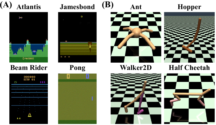
Figure 4: Atari games and MuJoCo environments in the OpenAI gym. (A) Screenshots from various Atari games. The agent needs to be alive and earn more rewards. (B) MuJoCo robot control tasks, making robots of different shapes walk forward as fast as possible.

4 Experiments

In this section, we apply the ACSF to both online and offline methods and evaluate them in different environments. We compared the ACSF with the latest SRL methods to prove that the ACSF can achieve a better trade-off between performance and latency. We also conduct ablation studies to demonstrate the superiority of adaptive coders.

4.1 Experimental Settings

4.1.1 Environment

To evaluate the proposed ACSF, we apply it to sixteen Atari 2600 games from the arcade learning environment (ALE) Bellemare et al. (2013) and four MuJoCo Todorov et al. (2012) continuous robot control tasks from the OpenAI gym Brockman et al. (2016). We use the most stable version of the Atari game without frame skipping (NoFrameskip-v4) and the latest version of the MuJoCo environment (-v3). The visualization of environments is shown in Figure 4. The training steps for Atari games and MuJoCo environments are 50 million (50M) and 1 million (1M), respectively, and the evaluation interval is 50 thousand (50K) and 5 thousand (5K).

4.1.2 Training and Evaluating

Baseline methods DQN, DDPG, BCQ, BC, and the proposed ACSF were all trained using the same structure as in Fujimoto et al. (2019). Our results are reported over 5 random seeds Duan et al. (2016) of the behavioral policy, the OpenAI gym simulator, and network initialization. We save the model with the highest average reward for testing.

We evaluate the ACSF on Atari games by playing 10 rounds of each game with an $\epsilon$-policy ($\epsilon=0.05$). Each episode is evaluated for up to 18K frames per round. To test the robustness of the agent in different situations, the agent starts with a random number (at most 30 times) of no-op actions. For MuJoCo environments, we played 10 rounds of each environment without exploration, and each test episode lasted for a maximum of 1K frames.

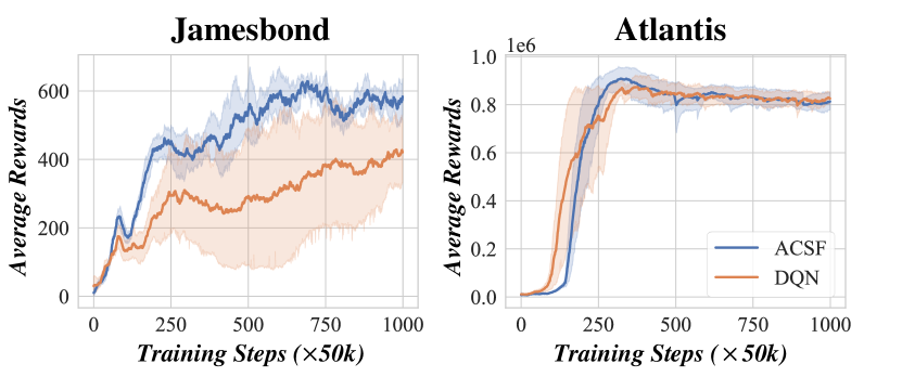
Figure 5: Learning curves for DQN and ACSF. During the training process, the performance of ACSF meets or exceeds that of the DQN algorithm. The learning curves have been smoothed for aesthetics.

4.2 Results on Atari Games

To test the performance of ACSF on game controls (a discrete action-space environment), we apply it to the DQN algorithm and test it on 16 different Atari games. We also compare the ACSF with some other DSQN methods Tan et al. (2021); Liu et al. (2022); Chen et al. (2022) to show it can achieve an excellent trade-off between latency and performance.

The experimental results and comparisons are shown in Table 1 and Figure 5. The full learning curves are included in the supplementary material. Experimental results show that ACSF outperforms the original DNQ algorithm. Meanwhile, compared to other SNN-based methods, ACSF maintains similar or better performance and reduces latency by more than 50%. This also proves that adaptive coding performs better on RL tasks than fixed coding.

4.3 Results on MuJoCo Robot Control Tasks

The ACSF is a complete SRL framework that can be applied to both online and offline algorithms. Therefore, we apply ACSF to offline algorithms and conduct experiments in a discrete action-space environment to prove the versatility of ACSF. We compare the performance of ACSF with three baseline algorithms (DDPG, BC, BCQ). The results are shown in Table 2 and Figure 6. From the results, ACSF is also suitable for offline algorithms, and the adaptive coders improve the performance significantly. Even at ultra-low latency ($T=4$), ACSF outperformed all the baseline algorithms.

The performance of ACSF will also vary under different time step settings because the latency ($T$) affects the dimension of the learnable matrix in adaptive coders, and thus affects the fitting ability of coders. According to experimental results, ACSF can achieve its best performance when $T=8$ or $T=10$. We can select the value of $T$ flexibly according to the usage scenario.

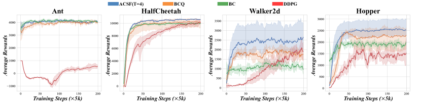
Figure 6: Learning curves for different algorithms in the MuJoCo environment.

Method	DDPG	BC	BCQ	ACSF	ACSF	ACSF	ACSF
Time Step	-	-	-	$T=4$	$T=6$	$T=8$	$T=10$
Ant	542 $\pm$ 192	4052 $\pm$ 28	3959 $\pm$ 546	4100 $\pm$ 323	4526 $\pm$ 152	4598 $\pm$ 106	4567 $\pm$ 140
HalfCheetah	10066 $\pm$ 469	9978 $\pm$ 128	8430 $\pm$ 152	10610 $\pm$ 63	10960 $\pm$ 229	10983 $\pm$ 215	10913 $\pm$ 292
Walker2d	1917 $\pm$ 380	1103 $\pm$ 161	1770 $\pm$ 277	2551 $\pm$ 932	3545 $\pm$ 1680	4103 $\pm$ 1728	4589 $\pm$ 421
Hopper	1450 $\pm$ 320	1888 $\pm$ 105	2261 $\pm$ 603	2527 $\pm$ 455	2805 $\pm$ 919	3024 $\pm$ 663	3211 $\pm$ 639

Table 2: Average reward for MuJoCo environments.

4.4 Ablation Study

To verify that adaptive coders can improve performance effectively. We conducted ablation experiments to compare the performance of algorithms with different coding methods. We compared five settings:

• No coders+DNN: The original BCQ algorithm.

• Rate coders+SNN: Compute the firing rate of spikes as the value function.

• Accumulate coders+SNN: Modify the dynamics of the output neurons to make them stop firing spikes. Record the voltage at the last time step as the value function.

• Adaptive coders+DNN: On the basis of the original DNN, adaptive coders are added to eliminate the bias caused by the structural differences introduced by the adaptive coders.

• Adaptive coders+SNN: Combines adaptive coders and directly-trained SNNs (the proposed ACSF).

Settings	Ant	HalfCheetah	Walker2d	Hopper
None+DNN	3959 $\pm$ 546	8430 $\pm$ 152	1770 $\pm$ 277	2261 $\pm$ 603
Rate+SNN†	-498 $\pm$ 155	-95 $\pm$ 103	251 $\pm$ 40	99 $\pm$ 6
Accum.+SNN†	3993 $\pm$ 490	9854 $\pm$ 196	1942 $\pm$ 416	2459 $\pm$ 259
Adapt.+DNN†	4076 $\pm$ 313	9960 $\pm$ 124	2080 $\pm$ 567	2268 $\pm$ 247
Adapt.+SNN†	4100 $\pm$ 323	10610 $\pm$ 63	2551 $\pm$ 932	2527 $\pm$ 455

• The time step is set to $T=4$.

Table 3: The performance of different coders.

Table 3 displays the results. Rate encoding does not work well due to very short time steps. The accumulate coders lose their spike characteristics, so the performance is better and similar to that of pure DNN. The combination of adaptive coders and DNN is slightly superior to pure DNN, which also proves that adaptive coders can integrate state information and calculate the value function accurately. The combination of adaptive coders and SNN has optimal performance in different environments, demonstrating the effectiveness of ACSF in low-latency settings.

4.5 Power Estimation and Comparison

To calculate the power consumption of SNNs on hardware, we count the total synaptic operations (SynOps) Wu et al. (2021). It is defined as follows:

$$\begin{split}SynOps=\sum_{t=1}^{T}\sum_{l=1}^{L-1}\sum_{j=1}^{N^{l}}f_{out,j}^{l}s_{j}^{l}[t]\end{split}$$ (20)

where $f_{out}$ denotes the number of outgoing connections to the subsequent layer, $T$ denotes the total time steps, $L$ is the total number of layers, $N^{l}$ means the number of neurons in layer $l$, and $s$ denotes the spikes.

For DNNs:

$$\begin{split}SynOps=\sum_{l=1}^{L}f_{in}^{l}N^{l}\end{split}$$ (21)

where $f_{in}^{l}$ represents the number of incoming connections to each neuron in layer $l$.

Algorithm	DQN		BCQ
Framework	DNN	ACSF	DNN	ACSF
SynOps	1.6M	288.8K	413.7K	277.9K
Energy Saved	-	81.95%	-	32.83%

Table 4: Total synaptic operations.

The total SynOps are shown in Table 4. The ACSF improves energy efficiency (up to 5X) on both algorithms, providing a more efficient application method for DRL.

5 Conclusion

In this paper, we propose a low latency adaptive coding spike framework (ACSF) for SRL. The ACSF solves the high latency problem in SRL by using adaptive coding. At the same time, ACSF has expanded the application range of SRL by designing structures for online and offline algorithms. In terms of versatility, ACSF is the first model to achieve compatibility with both online and offline algorithms and achieve optimal performance in both discrete and continuous environments. In addition, ACSF uses a directly trained SNN, which does not require DNNs, so it can be easily migrated to neuromorphic hardware. Extensive experiments show that ACSF can achieve the same or higher performance with ultra-low latency compared to other SRL methods. Meanwhile, compared with traditional DRL methods, ACSF has a significant improvement on inference energy efficiency (up to 5X) while maintaining better performance.

References

- Arulkumaran et al. [2017] Kai Arulkumaran, Marc Peter Deisenroth, Miles Brundage, and Anil Anthony Bharath. A brief survey of deep reinforcement learning. CoRR, abs/1708.05866, 2017.
- Bellec et al. [2020] Guillaume Bellec, Franz Scherr, Anand Subramoney, Elias Hajek, Darjan Salaj, Robert Legenstein, and Wolfgang Maass. A solution to the learning dilemma for recurrent networks of spiking neurons. Nature Communications, 11:1–15, 2020.
- Bellemare et al. [2013] Marc G Bellemare, Yavar Naddaf, Joel Veness, and Michael Bowling. The arcade learning environment: An evaluation platform for general agents. In Proceedings of the 24th International Joint Conference on Artificial Intelligence, pages 253–279, 2013.
- Bing et al. [2018] Zhenshan Bing, Claus Meschede, Kai Huang, Guang Chen, Florian Rohrbein, Mahmoud Akl, and Alois Knoll. End to end learning of spiking neural network based on R-STDP for a lane keeping vehicle. In 2018 IEEE International Conference on Robotics and Automation, pages 1–8, 2018.
- Brockman et al. [2016] Greg Brockman, Vicki Cheung, Ludwig Pettersson, Jonas Schneider, John Schulman, Jie Tang, and Wojciech Zaremba. Openai gym. CoRR, abs/1606.01540, 2016.
- Chen et al. [2022] Ding Chen, Peixi Peng, Tiejun Huang, and Yonghong Tian. Deep reinforcement learning with spiking q-learning. CoRR, abs/2201.09754, 2022.
- Duan et al. [2016] Yan Duan, Xi Chen, Rein Houthooft, John Schulman, and Pieter Abbeel. Benchmarking deep reinforcement learning for continuous control. In Proceedings of the 33nd International Conference on Machine Learning, pages 1329–1338, 2016.
- Frémaux et al. [2013] Nicolas Frémaux, Henning Sprekeler, and Wulfram Gerstner. Reinforcement learning using a continuous time actor-critic framework with spiking neurons. PLoS Computational Biology, 9:e1003024, 2013.
- Fujimoto et al. [2018] Scott Fujimoto, Herke van Hoof, and David Meger. Addressing function approximation error in actor-critic methods. In Proceedings of the 35th International Conference on Machine Learning, pages 1582–1591, 2018.
- Fujimoto et al. [2019] Scott Fujimoto, David Meger, and Doina Precup. Off-policy deep reinforcement learning without exploration. In Proceedings of the 36th International Conference on Machine Learning, pages 2052–2062, 2019.
- Girshick [2015] Ross Girshick. Fast R-CNN. In Proceedings of the 2015 IEEE International Conference on Computer Vision, pages 1440–1448, 2015.
- Hagenaars et al. [2021] Jesse J. Hagenaars, Federico Paredes-Vallés, and Guido de Croon. Self-supervised learning of event-based optical flow with spiking neural networks. In Advances in Neural Information Processing Systems 34, pages 7167–7179, 2021.
- Hu et al. [2021] Siyi Hu, Fengda Zhu, Xiaojun Chang, and Xiaodan Liang. Updet: Universal multi-agent RL via policy decoupling with transformers. In Proceedings of the 9th International Conference on Learning Representations, 2021.
- Kingma and Welling [2014] Diederik P Kingma and Max Welling. Auto-encoding variational bayes. In Proceedings of the 2nd International Conference on Learning Representations, 2014.
- Lahijanian et al. [2018] Morteza Lahijanian, Maria Svorenova, Akshay A Morye, Brian Yeomans, Dushyant Rao, Ingmar Posner, Paul Newman, Hadas Kress-Gazit, and Marta Kwiatkowska. Resource-performance tradeoff analysis for mobile robots. IEEE Robotics and Automation Letters, 3:1840–1847, 2018.
- Legenstein et al. [2008] Robert Legenstein, Dejan Pecevski, and Wolfgang Maass. A learning theory for reward-modulated spike-timing-dependent plasticity with application to biofeedback. PLoS Computational Biology, 4:e1000180, 2008.
- Li et al. [2021] Yuhang Li, Yufei Guo, Shanghang Zhang, Shikuang Deng, Yongqing Hai, and Shi Gu. Differentiable spike: Rethinking gradient-descent for training spiking neural networks. In Advances in Neural Information Processing Systems 34, pages 23426–23439, 2021.
- Li et al. [2022] Wenshuo Li, Hanting Chen, Jianyuan Guo, Ziyang Zhang, and Yunhe Wang. Brain-inspired multilayer perceptron with spiking neurons. In Proceedings of the 2022 IEEE/CVF Conference on Computer Vision and Pattern Recognition, pages 783–793, 2022.
- Lillicrap et al. [2016] Timothy P Lillicrap, Jonathan J Hunt, Alexander Pritzel, Nicolas Heess, Tom Erez, Yuval Tassa, David Silver, and Daan Wierstra. Continuous control with deep reinforcement learning. In Proceedings of the 4th International Conference on Learning Representations, 2016.
- Liu et al. [2022] Guisong Liu, Wenjie Deng, Xiurui Xie, Li Huang, and Huajin Tang. Human-level control through directly trained deep spiking -networks. IEEE Transactions on Cybernetics, pages 1–12, 2022.
- Maass [1997] Wolfgang Maass. Networks of spiking neurons: The third generation of neural network models. Neural Networks, 10:1659–1671, 1997.
- Mnih et al. [2015] Volodymyr Mnih, Koray Kavukcuoglu, David Silver, Andrei A Rusu, Joel Veness, Marc G Bellemare, Alex Graves, Martin Riedmiller, Andreas K Fidjeland, Georg Ostrovski, et al. Human-level control through deep reinforcement learning. Nature, 518:529–533, 2015.
- Neftci and Averbeck [2019] Emre O. Neftci and Bruno B. Averbeck. Reinforcement learning in artificial and biological systems. Nature Machine Intelligence, 1:133–143, 2019.
- Niroui et al. [2019] Farzad Niroui, Kaicheng Zhang, Zendai Kashino, and Goldie Nejat. Deep reinforcement learning robot for search and rescue applications: Exploration in unknown cluttered environments. IEEE Robotics and Automation Letters, 4:610–617, 2019.
- Patel et al. [2019] Devdhar Patel, Hananel Hazan, Daniel J Saunders, Hava T Siegelmann, and Robert Kozma. Improved robustness of reinforcement learning policies upon conversion to spiking neuronal network platforms applied to atari breakout game. Neural Networks, 120:108–115, 2019.
- Shrestha and Orchard [2018] Sumit Bam Shrestha and Garrick Orchard. SLAYER: spike layer error reassignment in time. In Advances in Neural Information Processing Systems 31, pages 1419–1428, 2018.
- Silver et al. [2016] David Silver, Aja Huang, Chris J. Maddison, Arthur Guez, Laurent Sifre, George van den Driessche, Julian Schrittwieser, Ioannis Antonoglou, Vedavyas Panneershelvam, Marc Lanctot, Sander Dieleman, Dominik Grewe, John Nham, Nal Kalchbrenner, Ilya Sutskever, Timothy P. Lillicrap, Madeleine Leach, Koray Kavukcuoglu, Thore Graepel, and Demis Hassabis. Mastering the game of go with deep neural networks and tree search. Nature, 529:484–489, 2016.
- Sutton et al. [1999] Richard S Sutton, David McAllester, Satinder Singh, and Yishay Mansour. Policy gradient methods for reinforcement learning with function approximation. In Advances in Neural Information Processing Systems 12, pages 1057–1063, 1999.
- Tan et al. [2021] Weihao Tan, Devdhar Patel, and Robert Kozma. Strategy and benchmark for converting deep q-networks to event-driven spiking neural networks. In Proceedings of the 35th AAAI conference on artificial intelligence, pages 9816–9824, 2021.
- Tang et al. [2020] Guangzhi Tang, Neelesh Kumar, and Konstantinos P Michmizos. Reinforcement co-learning of deep and spiking neural networks for energy-efficient mapless navigation with neuromorphic hardware. In 2020 IEEE/RSJ International Conference on Intelligent Robots and Systems, pages 6090–6097, 2020.
- Todorov et al. [2012] Emanuel Todorov, Tom Erez, and Yuval Tassa. Mujoco: A physics engine for model-based control. In 2012 IEEE/RSJ International Conference on Intelligent Robots and Systems, pages 5026–5033, 2012.
- Wu et al. [2018] Yujie Wu, Lei Deng, Guoqi Li, Jun Zhu, and Luping Shi. Spatio-temporal backpropagation for training high-performance spiking neural networks. Frontiers in Neuroscience, 12:331, 2018.
- Wu et al. [2021] Jibin Wu, Yansong Chua, Malu Zhang, Guoqi Li, Haizhou Li, and Kay Chen Tan. A tandem learning rule for effective training and rapid inference of deep spiking neural networks. IEEE Transactions on Neural Networks and Learning Systems, pages 1–15, 2021.
- Yuan et al. [2019] Mengwen Yuan, Xi Wu, Rui Yan, and Huajin Tang. Reinforcement learning in spiking neural networks with stochastic and deterministic synapses. Neural Computation, 31:2368–2389, 2019.
- Zhang et al. [2022] Duzhen Zhang, Tielin Zhang, Shuncheng Jia, and Bo Xu. Multiscale dynamic coding improved spiking actor network for reinforcement learning. In Proceedings of the 36th AAAI conference on artificial intelligence, pages 59–67, 2022.