Shot noise as a characterization of strongly correlated metals

Abstract

Shot noise measures out-of-equilibrium current fluctuations and is a powerful tool to probe the nature of current-carrying excitations in quantum systems. Recent shot noise measurements in the heavy fermion strange metal YbRh₂Si₂ exhibit a strong suppression of the Fano factor ($F$) – the ratio of the current noise to the average current in the DC limit. This system is representative of metals in which electron correlations are extremely strong. Here we carry out the first theoretical study on the shot noise of diffusive metals in the regime of strong correlations. A Boltzmann-Langevin equation formulation is constructed in a quasiparticle description in the presence of strong correlations. We find that $F=\sqrt{3}/{4}$ in such a correlation regime. Hence, the Fano factor suppression observed in experiments on YbRh₂Si₂ necessitates a loss of the quasiparticles. Our work opens the door to systematic theoretical studies of shot noise as a means of characterizing strongly correlated metallic phases and materials.

Introduction:

It is standard to describe metallic systems with electron correlations in terms of quasiparticles. These are elementary excitations that carry the quantum numbers of a bare electron, including charge $e$. In strange metals near quantum criticality Keimer and Moore (2017); Paschen and Si (2021), however, the current carriers are expected to lose Hu et al. (2022); Phillips et al. (2022) a well-defined quasiparticle interpretation and hence the notion of a discrete charge. This issue is especially pronounced in quantum critical heavy fermion metals Paschen and Si (2021); Kirchner et al. (2020); Coleman and Schofield (2005); Stewart (2001), for which a beyond-Landau description involving Kondo destruction Si et al. (2001); Coleman et al. (2001); Senthil et al. (2004) has received considerable experimental support Paschen et al. (2004); Friedemann et al. (2010); Shishido et al. (2005); Schröder et al. (2000); Aronson et al. (1995); Prochaska et al. (2020).

How to directly prove that quasiparticles are lost in correlated metals is largely an open question. One established means of such a characterization is in terms of the ratio of the thermal and electrical conductivities ($\kappa$ and $\sigma$, respectively). The quasiparticle description requires that the Lorenz number, $L\equiv\kappa/T\sigma$, obeys the Wiedemann-Franz law Chester and Thellung (1961); Castellani et al. (1987). Given that charge-neutral excitations such as phonons also contribute to the thermal current, alternative means of characterizing the absence of quasiparticles are much called for. Here we address this issue in terms of shot noise Blanter and Buttiker (2000), out-of-equilibrium fluctuations of the electrical current.

When electron correlations are strong, the shot noise of diffusive metals has not been theoretically considered. Here we show that, in such a regime of strong correlations and with a suitable requirement on a hieararchy of length scales, the quasiparticle description fails when the shot noise Fano factor ($F$), defined as the ratio of average current fluctuations in the static limit to the average current, disobeys $F=\sqrt{3}/4$.

Shot noise has proven invaluable in understanding several correlated electronic systems and materials such as quantum hall liquids, superconductors and quantum dots, and has offered a window into the nature of elementary charge carriers in their respective ground states Kobayashi and Hashisaka (2021). For example, measurement of the shot noise Fano factor has been pivotal in uncovering the $\frac{1}{3}$ charge fractionalization in the Laughlin state De-Picciotto et al. (1998); Saminadayar et al. (1997) and charge 2$e$ Cooper pairs in (fluctuating) superconductors Zhou et al. (2019); Bastiaans et al. (2021). Furthermore, the Fano factor has been widely used to isolate dominant scattering mechanisms in mesoscopic systems. Typically, in a diffusive Fermi gas, $F=\frac{1}{3}$ when scattering is dominated by impurities Beenakker and Buttiker (1992); Nagaev (1992). In a similar Fermi-gas-based approach, when the inelastic electron-electron scattering rate is allowed for and higher than the elastic scattering rate, but in the absence of significant electron-phonon scattering, $F$ was shown to equal $\frac{\sqrt{3}}{4}$ Kozub and Rudin (1995); Nagaev (1995).

Recently, shot noise measurements in mesoscopic wires of the heavy fermion compound YbRh₂Si₂ showed a large suppression of the Fano factor well below that of a Fermi-gas-based diffusive metal Chen et al. (2022). This was found to occur at low enough temperatures ($<10$K) where equilibration of electrons via a bosonic bath such as phonons is minimal, and cannot account for the reduced shot noise signal. Since the only other source of inelastic scattering is strong electron interactions, a natural question arises: can strong correlation effects in a Fermi liquid (FL) account for the observed shot noise suppression, or is it a signature of strange metallicity near the quantum critical point? This issue is particularly important, given that, even for the FL state of heavy fermion metals, the effect of interactions is pronounced and can induce orders-of-magnitude renormalization of both the quasiparticle weight and effective interactions.

Here we report on the first theoretical study about the shot noise of strongly correlated diffusive metals. We show that, in the presence of strong correlations, the Fano factor of a diffusive FL $F$ is equal to $\frac{\sqrt{3}}{4}$. In particular, it is independent of quasiparticle weight or Landau FL parameters. It includes, for example, the case when the quasiparticle residue $z_{\textbf{k}}$ approaches an infinitesimally small (but nonzero) value, or when the Landau parameters are as large as in the heavy fermion metals (typically about $\sim 10^{3}$). Since the existence of quasiparticles is central to the robustness of the Fano factor prediction, the experimentally observed suppression Chen et al. (2022) strongly indicates a loss of quasiparticles.

To this end, we derive the Boltzmann-Langevin transport equation for a diffusive metal in a regime suitable for addressing strong correlations. This allows us to analyze the role of strong interactions on the Fano factor. First, we notice that charge conservation constrains the Boltzmann equation to be independent of the quasiparticle weight. This holds even in the presence of anisotropic effects when $z_{\textbf{k}}$ is strongly momentum dependent. As a consequence, the current noise, average current, and Fano factor determined from the Boltzmann-Langevin equation are independent of $z_{\textbf{k}}$. Second, we calculate the shot noise, and demonstrate that the shot noise and average current get renormalized identically by the Landau parameters. As a result, the Fano factor remains robust to the introduction of arbitrarily strong interactions within FL theory. Also inherent in this cancellation is our observation that the conductance entering both shot noise and average current are equal and determined by the same quasiparticle lifetime, i.e., there is a symmetry of the scattering rate between single and multi-particle operators. This symmetry exists because in FLs, the interactions are instantaneous (no frequency dependence) and the electron scattering processes are Poissonian, i.e., independent of one another.

(a)

(b)

Figure 1: (a) Plot of the spectral function $A(\omega,\textbf{k})$ with k located at the Fermi momentum $\textbf{k}_{F}$. The area of the peak is determined by $z_{\textbf{k}}$. (b) A representation of the irreducible vertex contributing to the total vertex in the Bethe-Salpeter equation in Fig. 2(b) .

In the remainder of the paper, we construct the Boltzmann-Langevin equation in the strongly correlated regime of a FL. We closely follow the diagrammatic analysis of Betbeder-Matibet and Nozieres Betbeder-Matibet and Nozieres (1966). In particular, we analyze the role of interactions via coupling through the scalar and vector potentials. We then calculate the Fano factor through the shot noise and average current, and discuss its relevance to experiments in YbRh₂Si₂ before presenting our conclusions.

Boltzmann-Langevin equation for interacting Fermi liquids:

Interacting electrons in the presence of randomly distributed impurities is governed by the Hamiltonian, $H=H_{0}+H_{I}+H_{imp}$. Here $H_{0}=\sum_{\textbf{k},\sigma}\epsilon_{\textbf{k}}c_{\textbf{k}\sigma}^{\dagger}c_{\textbf{k}\sigma}$, $H_{I}=\frac{1}{2}\sum_{\begin{subarray}{c}\textbf{k},\textbf{k}^{\prime},\textbf{q}\\ \sigma\sigma^{\prime}\end{subarray}}V(\textbf{q})c_{\textbf{k}+\textbf{q}\sigma}^{\dagger}c_{\textbf{k}^{\prime}-\textbf{q}\sigma^{\prime}}^{\dagger}c_{\textbf{k}^{\prime}\sigma^{\prime}}c_{\textbf{k}\sigma}$ describe the non-interacting electron dispersion and Coulomb interaction, respectively. In addition, $H_{imp}=\sum_{i,\textbf{k},\textbf{q},\sigma}U(\textbf{q})e^{-i\textbf{q}\cdot\textbf{R}_{i}}c^{\dagger}_{\textbf{k}+\textbf{q}\sigma}c_{\textbf{k}\sigma}$ marks electron scattering from dilute impurities. The bare electron operator is denoted by $c_{\mathbf{k}\sigma}$ with $\mathbf{k}$ and $\sigma$ representing momentum and spin. The Coulomb and impurity matrix elements are denoted by $V(\textbf{q})$ and $U(\textbf{q})$, respectively. Next we consider an external field with Fourier components $\lambda(\textbf{k})$ that couples to the interacting electrons, which contributes

$$H^{\prime}(\mathbf{q}_{0},\omega_{0})=\sum_{\textbf{k},\sigma}\lambda_{\sigma}(\textbf{k})c^{\dagger}_{\textbf{k}+\textbf{q}_{0}/2\sigma}c_{\textbf{k}-\textbf{q}_{0}/2\sigma}e^{-i\omega_{0}t}+\mbox{h.c.},$$ (1)

to the total Hamiltonian, where $(\omega_{0},\textbf{q}_{0})\equiv q_{0}$ is the energy and momentum transfer between the electrons and the external field.

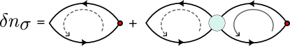
(a)

(b)

Figure 2: Diagrammatic representations of the key processes contributing to the Boltzman equation. (a) Density response. The dashed (solid) arrow indicates sum over internal frequency (frequency, momenta, and spin). The smaller/red (larger/cyan) filled disk represents the external field, $\lambda$, that elicits the density response (total 4-fermion vertex, $\Gamma$). (b) The Bethe-Salpeter equation for $\Gamma$ in terms of the irreducible vertex.

To see how the external field modifies the local electronic density to linear order, we write a semi-classical total density as $n_{\sigma}(k,\textbf{r},t)=n_{\sigma}^{0}(\textbf{k})+\delta n_{\sigma}(k,\textbf{q}_{0})e^{i(\textbf{q}_{0}\cdot\textbf{r}-\omega_{0}t)}+\mbox{h.c.}$. Here $k\equiv(\textbf{k},\Omega)$ is the average momentum and energy of the incoming particles. We have further defined variation of the density as the expectation value, $\delta n_{\sigma}(\textbf{k},q_{0})=\langle\psi(q_{0})|\alpha^{\dagger}_{\textbf{k}-\frac{1}{2}\textbf{q}_{0}\sigma}\alpha_{\textbf{k}+\frac{1}{2}\textbf{q}_{0}\sigma}|\psi(q_{0})\rangle$, where $\alpha_{\textbf{k}\sigma}$ is the quasiparticle operator, and $|\psi(q_{0})\rangle=|\psi_{0}\rangle+|\delta\psi(q_{0})\rangle$ is the ground state $|\psi_{0}\rangle$ corrected by $|\delta\psi\rangle$ due to the external field. The density response, $\delta n_{\sigma}(\textbf{k},q_{0})=\frac{1}{2\pi i}\int d\Omega\chi_{\sigma}(k,q_{0})$, can be evaluated using the diagram in Fig. 2(a), and it is given by

$$\chi_{\sigma}(k,q_{0})=z_{\textbf{k}}^{-1}\Lambda_{\sigma}(k,q_{0})G\left(k^{-}\right)G\left(k^{+}\right).$$ (2)

Here $z_{\textbf{k}}$ is the quasiparticle residue and is obtained by converting the quasiparticle operators in terms of the physical electron operators. $G(k^{\pm})\propto z_{\textbf{k}}$ are the interacting propagators for shifted wave vector and energies $k^{\pm}\equiv(\textbf{k}\pm\frac{1}{2}\textbf{q}_{0},\Omega\pm\frac{1}{2}\omega)$. Scatterings among electrons renormalize $\lambda_{\sigma}$ [red disk in Fig. 2(a)] to $\Lambda_{\sigma}$, which is given by

$$\Lambda_{\sigma}(k,q_{0})=\lambda_{\sigma}(\textbf{k})$$

$$\qquad+\sum_{\textbf{k}^{\prime}\sigma^{\prime}\Omega^{\prime}}\lambda_{\sigma^{\prime}}(\textbf{k}^{\prime})\Gamma_{\sigma,\sigma^{\prime}}(k,k^{\prime},q_{0})G\left(k^{-}\right)G\left(k^{+}\right),$$ (3)

where $\Gamma_{\sigma,\sigma^{\prime}}$ is the fully dressed 4-fermion vertex. In order to include renormalizations from both electron-electron and electron-impurity scatterings, we utilize the Bethe-Salpeter equation [see Fig. 2(b)] to obtain $\Gamma_{\sigma,\sigma^{\prime}}(k,k^{\prime},q_{0})=\hat{\Gamma}_{\sigma,\sigma^{\prime}}(k,k^{\prime},q_{0})+\Delta\Gamma_{\sigma,\sigma^{\prime}}(k,k^{\prime},q_{0})$ where

$$\Delta\Gamma_{\sigma,\sigma^{\prime}}(k,k^{\prime},q_{0})=\sum_{\begin{subarray}{c}\textbf{k}^{\prime\prime}\sigma^{\prime\prime}\\ \Omega^{\prime\prime}\end{subarray}}\hat{\Gamma}_{\sigma,\sigma^{\prime\prime}}(k,k^{\prime\prime},q_{0})$$

$$\times G\left(k^{\prime\prime-}\right)G\left(k^{\prime\prime+}\right)\Gamma_{\sigma^{\prime\prime},\sigma^{\prime}}(k^{\prime\prime},k^{\prime},q_{0})$$ (4)

and $\hat{\Gamma}_{\sigma,\sigma^{\prime}}(k,k^{\prime},q_{0})$ (Fig. 1) is the sum of all irreducible vertex diagrams including Coulomb and impurity scatterings.

Eliminating the vertex part $\Lambda_{\sigma}(k,q_{0})$ [Eq. (3)] between the density response [Fig. 2(a)] and the Bethe-Salpeter equation [Fig. 2(b)] in favor of the irreducible vertex $\hat{\Gamma}_{\sigma,\sigma^{\prime}}(k,k^{\prime},q_{0})$, we obtain the Boltzmann transport equation for the quasiparticles,

$$dn_{\bm{p}}(\bm{x},t)/dt+I(n_{\bm{p}})=0$$ (5)

with $d/dt=\partial_{t}+\dot{\bm{x}}\cdot\partial_{\bm{x}}\dot{\bm{p}}\cdot\partial_{\bm{p}}$, where $\dot{\bm{x}}=\partial\epsilon_{p}/\partial\bm{p}=\bm{v},\dot{\bm{p}}=-\partial\epsilon_{p}/\partial\bm{x}=e\bm{E}-\sum_{\bm{p}^{\prime}}f_{\bm{p},\bm{p}^{\prime}}\partial_{\bm{x}}\delta n_{\bm{p}^{\prime}}$, and

$$\epsilon_{\bm{p}}(x)=\epsilon_{\bm{p}}^{0}-e\bm{E}\cdot\bm{x}+\sum_{\bm{p}^{\prime}}f_{\bm{p},\bm{p}^{\prime}}\delta n_{\bm{p}^{\prime}}$$ (6)

denotes the total quasiparticle energy. $\epsilon^{0}_{\bm{p}}$ corresponds to the quasiparticle energy at global equilibrium. $\bm{v}$ denotes the quasiparticle velocity, $\bm{E}$ refers to the static electric field acting on the quasiparticles. $I(n_{\bm{p}})=I_{im}+I_{ee}$ consists of electron-impurity and electron-electron collision integrals. Note that the vertex parts can be solved exactly in the static long-wavelength limit of $\textbf{q}_{0},\omega_{0}\rightarrow 0$ with constant $|\textbf{q}_{0}|/\omega_{0}$ Betbeder-Matibet and Nozieres (1966). Since the Ward identities constrain $\Lambda_{\textbf{k}}\propto z_{\textbf{k}}^{-1}$, it is clear from the expression of $\chi_{\sigma}(\textbf{k},\Omega,\textbf{q}_{0},\omega_{0})$ that the density response, and as a consequence the Boltzmann equation, are independent of the quasiparticle residue.

While the Boltzmann transport equation is useful to calculate the nonequilibrium average electronic behavior, it is insufficient to describe their fluctuations. To do this, we introduce a Langevin source term $\delta J^{ext}$ to the Boltzmann equationKogan and Shulman (1969), which allows the room for quasiparticle fluctuations $n_{\bm{p}}\rightarrow n_{\bm{p}}+\delta n^{fl}_{\bm{p}}$ to give the Boltzmann-Langevin equation for a strongly correlated Fermi liquid,

$$(\partial_{t}+\bm{v}\cdot\partial_{\bm{x}})\delta n_{\bm{p}}^{fl}(\bm{x},t)+\delta I$$

$$= \frac{\partial n_{0}}{\partial{{\epsilon}}}\bm{v}\cdot\sum_{p^{\prime}}f_{p,p^{\prime}}\partial_{\bm{x}}\delta n^{fl}_{p^{\prime}}+\delta J^{ext}(\bm{p},\bm{x},t).$$ (7)

Here $\delta I$ represents the change of collision integral due to fluctuating quasiparticles $\delta n_{p}^{fl}$. These fluctuations have zero mean value but have finite correlations. The electric field is absent in Eq. (S9) because of its higher order contribution $E\sim O(\delta n)$. $\delta J^{ext}$ denotes the extraneous flux of particles in $\bm{p}$ state and equals

$$\delta J^{ext}(p,x,t)=\sum_{\bm{p}^{\prime}}\delta J(p^{\prime}p,x,t)-\delta J(pp^{\prime},x,t).$$ (8)

It is the difference between flux from all $\bm{p}^{\prime}$ states to $\bm{p}$ state and flux from $\bm{p}$ state to all $\bm{p}^{\prime}$ states. We assume that the different fluxes are correlated when and only when the initial and final states are identical thereby following a Poisson distribution of the form

$$\langle\delta J(p_{1}p_{1}^{\prime},x_{1},t_{1})\delta J(p_{2}p_{2}^{\prime},x_{2},t_{2})\rangle$$

$$= LA\delta_{p_{1},p_{2}}\delta_{p_{1}^{\prime},p_{2}^{\prime}}\delta(x_{1}-x_{2})\delta(t_{1}-t_{2})J(p_{1}p_{1}^{\prime},x_{1},t_{1}),$$ (9)

where $J(p_{1}p_{1}^{\prime},x_{1},t_{1})$ is the mean flux of particles. The presence of the Dirac delta functions in space-time reflect the fact that the duration and spatial extent of collisions is much smaller than the the electron-electron scattering lifetime and scattering length respectively. We will use Eq. (S9) to calculate the shot noise below.

Steady state:

Consider a diffusive correlated metallic wire with length $L$ and cross section $A$ $(L\gg\sqrt{A})$. We model the correlated metallic wire as a strongly interacting diffusive Fermi liquid with an applied voltage. An applied voltage drives the metal into a nonequilibrium steady state. The static electric potential energy $\delta\mu(x)=e\phi(x)=e\bm{E}\cdot\bm{x}$ serves as an $s$ wave perturbation to the quasiparticle distribution at every position along the system. The kinetics for the nonequilibrium system could be described by Boltzmann transport equation (5) for the quasiparticles. The two ends of the wire stay in their own equilibrium: $n_{p}(\pm L/2,t)=f(\epsilon_{p}(\pm L/2),T_{bath}=0)$, which serves as the boundary conditions to the Boltzmann equation, where $f$ is the Fermi-Dirac distribution function.

In the steady state, $\partial n_{\bm{p}}/\partial t=0$. In order to solve Eq. (5), we expand the Boltzmann equation in terms of $\delta\bar{n}(\bm{x},\bm{p})=n_{\bm{p}}(\bm{x})-n_{0}(\bm{x},\epsilon)$ in the regime where $E_{F}\gg 1/\tau_{im}\gg 1/\tau_{ee}\gg D/L^{2}$. The first inequality corresponds to the condition for dilute impurities, and the following inequalities denote for the strong correlation regime. The distribution $n_{0}(\bm{x},\epsilon)$ stands for local equilibrium distribution and $\epsilon$ refers to true quasiparticle energy defined in Eq. (6). $\delta\bar{n}(\bm{x},\bm{p})$ corresponds to the departure from local equilibrium. This should be contrasted with the quasiparticle excitation $\delta n_{\bm{p}}(x)=n_{\bm{p}}(\bm{x})-n_{0}(\epsilon_{\bm{p}}^{0})$ in Eq. (6), where $n_{0}(\epsilon_{\bm{p}}^{0})$ refers to the distribution at global equilibrium without any position dependence. The two quantities are connected by $\delta\bar{n}(\bm{x},\bm{p})=\delta n_{\bm{p}}-\frac{\partial{n_{0}}}{\partial{\epsilon}}\sum_{\bm{p}^{\prime}}f_{\bm{p},\bm{p}^{\prime}}\delta n_{\bm{p}^{\prime}}(\bm{x})$. Only the local equilibrium distribution $n_{0}(\bm{x},\epsilon)$ as a function of real quasiparticle energy $\epsilon$ could make the collision integral $I=I_{im}+I_{ee}$ vanish, and only $\delta\bar{n}(\bm{x},\bm{p})$, rather than $\delta{n}_{\bm{p}}(\bm{x})$, determines the currentLifschitz and Pitajewski (1983); Betbeder-Matibet and Nozieres (1966).

At the zeroth order, effective $e-e$ scattering drives the quasiparticles into local equilibrium, with a general position dependent Fermi-Dirac form $n_{0}(\epsilon,x)=f(\epsilon,T(x))$ such that $I(n_{0})=0$. After the expansion, we get two equations in terms of $n_{0}$ and $\delta\bar{n}$,

$$\bm{v}\cdot\partial_{\bm{x}}n_{0}(\bm{x},\bar{\epsilon})+e\bm{E}\cdot\bm{v}\partial_{\epsilon}n_{0}=\frac{\delta\bar{n}}{\tau}$$ (10)

$$\bm{v}\cdot\partial_{\bm{x}}\delta\bar{n}+e\bm{E}\cdot\partial_{\bm{p}}\delta\bar{n}=0$$ (11)

where $\bar{\epsilon}=\epsilon_{\bm{p}}^{0}-e\bm{E}\cdot\bm{x}$ is the non-interacting quasiparticle energy without any Landau parameters. In the case where the conductance is mainly contributed by impurity scattering, $\tau_{im}\ll\tau_{ee}$, we can relace $\tau$ with $\tau_{im}$ in Eq. (10). Then we follow the analysis of Kozub and Rudin Kozub and Rudin (1995). Substituting Eq. (10) into (11), and integrating with $\bar{\epsilon}d\epsilon$. We note that $\epsilon$ and $\bar{\epsilon}$ in the distribution function have no explicit dependence on position. We get the diffusion equation in terms of the local equilibrium temperature at leading order in $E$,

$$\frac{\pi^{2}}{6}\frac{\partial^{2}}{\partial x^{2}}T^{2}(x)+(eE)^{2}=0$$ (12)

with boundary conditions $T(\pm L/2)=0$. Same as the equation in a Fermi gas Kozub and Rudin (1995); Nagaev (1995), the solution to Eq. (12) has the form

$$T(x)=\frac{\sqrt{3}}{2\pi}eV\sqrt{1-\left(\frac{2x}{L}\right)^{2}}$$ (13)

with $V=EL$. The local equilibrium distribution function $n_{0}=f(\epsilon,T(x))$ is plotted at zero and finite environment temperature in Fig. S1 in the supplementary material.

Shot noise:

To calculate the shot noise, we model the mean particle flux as $J(p^{\prime}p,x,t)=W(p^{\prime}p)n_{p^{\prime}}(x,t)(1-n_{p}(x,t))$, where $W(pp^{\prime})$ is the scattering rate, which in the isotropic case $W(pp^{\prime})=\delta({\epsilon_{p}-\epsilon_{p^{\prime}}})/(LAN_{F}\tau_{im})$. The extraneous flux of quasiparticles could be connected with the quasiparticle fluctuation and thereby connects with the current fluctuation through Boltzmann-Langevin equation (S9). We leave the details of the derivations to the supplementary material and list the final results of the current noise,

$$S=2\int_{-\infty}^{\infty}dt\langle\delta I(t)\delta I(0)\rangle=\frac{\sqrt{3}}{2}GeV$$ (14)

where $T(x)$ is the local temperature in Eq. (13). $G=e^{2}DN_{F}A/L=ne^{2}\tau_{im}A/(m^{*}L)$ represents the conductance of the FL.

We find that under electron correlation, the Landau parameters only renormalize the conductance. Therefore the Fano factor $F=S/2eI$ is still $\sqrt{3}/4$ compared with the Fermi gas results in the hot electron regime, regardless of the interaction strength.

Discussion:

Several remarks are in order. First, in our calculations, we assume that the corrections to the quasiparticle density and energies are linear in the external perturbation (linear response). The role of non-linearities in the response and the Fano factor dependence of the interaction parameters will be captured by higher order terms. Second, our calculations also assume intermediate mesoscopic length scales in accordance with experimental values. If the wire is too long, electron-phonon scattering must be considered, which acts to suppress the shot noise and Fano factor. If the length of the wire is much smaller than $L_{ee}$, inelastic scattering does not contribute to the shot noise and Fano factor is automatically independent of the interaction strength and Landau parameters. Third, when retardation effects become important, as for example in the limit of lower electron densities, the Poissonian nature of the interaction fails. In this case, one must revisit the issue of the Fano factor dependence on the interaction parameters. Finally, in experiments on YbRh₂Si₂, the mesoscopic wire is quasi-three dimensional where FL theory continues to hold. However, when the transverse dimensions of the wire are sufficiently reduced, FL theory eventually gives way to Luttinger liquid physics. In this case, the Fano factor generally depends on the dimensionless Luttinger liquid parameters since the shot noise responds to an effective charge $ge$ with $g$ being the interaction parameter Kane and Fisher (1994); Blanter and Buttiker (2000).

To conclude, we have shown that the Fano factor of a strongly correlated Fermi liquid, defined by the ratio of its average current fluctuations to its average current, equals that of a Fermi gas in the linear response regime. More specifically, our results demonstrate that the Poissonian nature of the instantaneous Coulomb interaction and charge conservation dictate a Fano factor that is independent of the Landau parameters or (however small) quasiparticle residue respectively. This has important consequences to recent shot noise experiments in the heavy fermion material YbRh₂Si₂ where a strong suppression of the Fano factor was observed even when the effect of electron-phonon coupling is negligible Chen et al. (2022). The existence of a quasiparticle interpretation is a sufficient requirement for our analysis to hold. Thus, any suppression of the Fano factor below that of a correlated diffusive metal ($F=\frac{\sqrt{3}}{4}$) strongly suggests the loss of quasiparticles in YbRh₂Si₂. More generally, our work points to shot noise Fano factor as a powerful characterization of strongly correlated metallic phases and materials.

Acknowledgements:

This work was supported in part by the Robert A. Welch Foundation Grant No. C-1411 (Y.W.), the Air Force Office of Scientific Research under Grant No. FA9550-21-1-0356 (C.S.) and the National Science Foundation under Grant No. DMR-2220603 (S.S. and Q.S.). L.C. and D. N. acknowledge support by US Department of Energy, Basic Energy Sciences, under award No. DE-FG02-06ER46337. S.P. acknowledges funding from the Austrian Science Fund (projects No. I4047, 29279 and the Research unit QUAST-FOR5249) and the European Microkelvin Platform (H2020 project No. 824109). Q.S. acknowledges the hospitality of the Aspen Center for Physics, which is supported by NSF grant No. PHY-1607611.

Appendix A Supplementary Material: Shot noise as a characterization of strongly correlated metals

A.1 Additional details for the derivation of the Boltzmann equation

As noted in the main text, the Boltzmann equation follows from eliminating the dressed external vertex, $\Lambda$, from the explicit expression of density fluctuation, $\delta n_{\sigma}$. Since we want to describe the dynamics of fluctuations that live on the Fermi surface, we seek a solution of the form Betbeder-Matibet and Nozieres (1966),

$$\delta n_{\sigma}(\mathbf{k},q_{0})=\nu(\hat{k},q_{0})\delta(\epsilon_{\mathbf{k}}-\mu),$$ (S1)

where $\hat{k}$ represents Fermi surface coordinates. This leads to

$$\delta n_{\sigma}(\mathbf{k},q_{0})=z_{\mathbf{k}}\delta(\epsilon_{\mathbf{k}}-\mu)\left[\frac{\Lambda^{1}_{\sigma}(\hat{k},q_{0})+\Lambda^{2}_{\sigma}(\hat{k},q_{0})}{2i\Gamma_{\text{imp}}+\omega_{0}-\mathbf{v}_{k}\cdot\mathbf{q}_{0}}\omega_{0}-\Lambda^{0}_{\sigma}(\hat{k},q_{0})\right],$$ (S2)

where $\Gamma_{\text{imp}}$ is the rate of scattering between the electrons and the impurities, $\Lambda_{\sigma}^{0}(\hat{k})$ is the solution for $\Lambda_{\sigma}(\hat{k},q_{0})$ at $\omega_{0}=0$, and $\Lambda^{1,2}_{\sigma}$ are obtained by solving the Bethe-Salpeter equation for $\Lambda_{\sigma}$, which takes the general form

$$\Lambda_{\sigma}(k,q_{0})=\Lambda_{\sigma}^{1}(k,q_{0})+\Lambda_{\sigma}^{2}(k,q_{0})\Theta(\omega_{0}-2|\Omega-\mu|).$$ (S3)

On the Fermi surface a recursive relationship for $\Lambda^{n}$’s is obtained Betbeder-Matibet and Nozieres (1966)

$$\Lambda_{\sigma}^{1}(\hat{k},q_{0})=\Lambda_{\sigma}^{0}(\hat{k})+\frac{\omega_{0}}{8\pi}\sum_{\sigma^{\prime}}\int d\hat{k}^{\prime}\frac{X_{\sigma,\sigma^{\prime}}(\hat{k},\hat{k}^{\prime})}{2i\Gamma_{\text{imp}}+\omega_{0}-\mathbf{v}_{k^{\prime}}\cdot\mathbf{q}_{0}}\left[\Lambda_{\sigma^{\prime}}^{1}(\hat{k}^{\prime},q_{0})+\Lambda_{\sigma^{\prime}}^{2}(\hat{k}^{\prime},q_{0})\right]$$ (S4)

$$\Lambda_{\sigma}^{2}(\hat{k},q_{0})=\frac{i}{2\pi}\int d\hat{k}^{\prime}\frac{Y(\hat{k},\hat{k}^{\prime})}{2i\Gamma_{\text{imp}}+\omega_{0}-\mathbf{v}_{k^{\prime}}\cdot\mathbf{q}_{0}}\left[\Lambda_{\sigma}^{1}(\hat{k}^{\prime},q_{0})+\Lambda_{\sigma}^{2}(\hat{k}^{\prime},q_{0})\right].$$ (S5)

Here $X_{\sigma,\sigma^{\prime}}(\hat{k},\hat{k}^{\prime})$ is a function of Fermi surface coordinates and fully determined by Landau parameters. By contrast, $Y(\hat{k},\hat{k}^{\prime})$ encodes contributions that exist only due to electron-impurity scatterings. By adding $\Lambda^{1}_{\sigma}$ and $\Lambda^{2}_{\sigma}$, we replace their sum in Eq. (S2) to obtain the Boltzmann equation in frequency-momentum space with the collision integral,

$$I(n_{\mathbf{k}})=2i\int\frac{d\hat{k}^{\prime}}{4\pi}Y(\hat{k},\hat{k}^{\prime})\delta\bar{n}(\mathbf{k}^{\prime})-2i\Gamma_{\text{imp}}\delta\bar{n}(\mathbf{k}),$$ (S6)

where $\bar{n}(\mathbf{k})$ is defined in the main text. In Eq. (4) we express the Boltzmann equation in real-time and coordinate space.

We note that the contribution to $I$ above entirely results from electron-impurity collisions. In our calculations we model it as

$$I_{im}=\sum_{p^{\prime}}W(pp^{\prime})[n_{p}(x,t)(1-n_{p^{\prime}}(x,t))-n_{p^{\prime}}(x,t)(1-n_{p}(x,t))],$$ (S7)

where $W$ refers to the scattering rate for electron-impurity collisions, and propotional to $Y$. In principle, electron-electron collisions also contribute to $I$, but they vanish on the Fermi surface at $T_{\text{bath}}=0$. An applied voltage, however, generates scatterings among electrons at $T_{\text{bath}}=0$, which results in a finite local temperature $T(x)$ [see Sec. II]. Consequently, $I$ acquires a contribution resulting from the applied voltage,

$$I_{ee}=\sum_{2,3,4}\widetilde{W}(12;34)\delta_{\bm{p}+\bm{p}_{2},\bm{p}_{3}+\bm{p}_{4}}\delta{(\epsilon+\epsilon_{2}-\epsilon_{3}-\epsilon_{4})}[n_{3}n_{4}(1-n_{1})(1-n_{2})-n_{1}n_{2}(1-n_{3})(1-n_{4})],$$ (S8)

where $\widetilde{W}$ refers to the transmission probability for electron-electron collisions. Thus, the net $I$ in the presence of an applied voltage is $I=I_{im}+I_{ee}$.

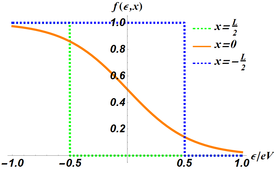
(a)

(b)

Figure S1: Plot of the local equilibrium distribution function with kinetic energy in the correlated metal with (a) $T_{bath}=0$, (b) $T_{bath}>0$ at $x=L/2$ (Green), $x=0$ (Orange) and $x=-L/2$ (Blue) respectively.

A.2 Fluctuations of the nonequilibrium Boltzmann-Langevin equation for a Fermi liquid

As described in the main text, the fluctuations of the nonequilibrium quasiparticles are described by the Boltzmann-Langevin equation:

$$(\partial_{t}+\bm{v}\cdot\partial_{\bm{x}})\delta n_{p}^{fl}(x,t)+\delta I=\frac{\partial n_{0}}{\partial{{\epsilon}}}\bm{v}\cdot\sum_{p^{\prime}}f_{p,p^{\prime}}\partial_{\bm{x}}\delta n^{fl}_{p^{\prime}}+\delta J^{ext}(p,x,t)\,$$ (S9)

where $\delta J^{ext}$ denotes the extraneous flux of the particles in $\bm{p}$ state, and $\delta I$ represents the change of the collision integral due to fluctuating quasiparticles. These fluctuations have finite correlations with zero mean values, $\langle\delta{n}^{fl}\rangle=\langle\delta I\rangle=\langle\delta J^{ext}\rangle=0$. Since the current is mainly contributed by the elastic collision $(\tau_{im}\ll\tau_{ee})$, we only consider flux from the elastic collisions,

$$I_{imp}= \sum_{p^{\prime}}J(p^{\prime}p)-J(pp^{\prime})$$ (S10)

$$J(p^{\prime}p,x,t)= W(p^{\prime}p)n_{p^{\prime}}(x,t)(1-n_{p}(x,t))$$ (S11)

where $W(pp^{\prime})$ is the scattering rate. In the isotropic case, it is given as follows:

$$W(pp^{\prime})=\frac{\delta(\epsilon_{p}-\epsilon_{p^{\prime}})}{LAN_{F}\tau_{im}}.$$ (S12)

The correlation of $\delta J^{ext}$ is determined only by the fact that each electron scattering event is independent of one another Kogan and Shulman (1969). Thus, each scattering is only self-correlated. The flux into the $\bm{p}$ state could be expressed by the subtraction between the flux from all $\bm{p}^{\prime}$ states to the $\bm{p}$ state and the flux from the $\bm{p}$ state to all $\bm{p}^{\prime}$ states,

$$\delta J^{ext}(p,x,t)=\sum_{\bm{p}^{\prime}}\delta J(p^{\prime}p,x,t)-\delta J(pp^{\prime},x,t)\,.$$ (S13)

Different fluxes are correlated when and only when the initial and final states are identical, following Poissonian statistics:

$$\langle\delta J(p_{1}p_{1}^{\prime},x_{1},t_{1})\delta J(p_{2}p_{2}^{\prime},x_{2},t_{2})\rangle=LA\delta_{p_{1},p_{2}}\delta_{p_{1}^{\prime},p_{2}^{\prime}}\delta(x_{1}-x_{2})\delta(t_{1}-t_{2})J(p_{1}p_{1}^{\prime},x_{1},t_{1})\,.$$ (S14)

Then

$$\langle\delta J^{ext}(p_{1},x_{1},t_{1})\delta J^{ext}(p_{2},x_{2},t_{2})\rangle=LA\delta(x_{1}-x_{2})\delta(t_{1}-t_{2})\{\delta_{p_{1},p_{2}}\sum_{q}[J(p_{1},q)+J(q,p_{1})]-J(p_{1},p_{2})-J(p_{2},p_{1})\}$$ (S15)

where $J(p_{1},p_{2})$ denotes the mean quasiparticle flux defined in Eq. (S11). The Boltzmann-Langevin equation (S9) could be re-expressed as

$$\partial_{t}\delta n^{fl}+\bm{v}\cdot\partial_{\bm{x}}\delta\bar{n}^{fl}+\delta I=\delta J^{ext},$$ (S16)

where $\delta\bar{n}_{p}^{fl}=\delta{n}_{p}^{fl}-\frac{\partial n_{0}}{\partial{\epsilon}}\sum_{p^{\prime}}f_{p,p^{\prime}}\partial_{x}\delta n_{p^{\prime}}^{fl}$, which is similar to the relation between $\delta n$ and $\delta\bar{n}$ in the Landau transport equation of a FL Lifschitz and Pitajewski (1983); Betbeder-Matibet and Nozieres (1966). Following the analysis of Nagaev Nagaev (1992), we express the fluctuation $\delta\bar{n}$ and the source as the sum of symmetric and antisymmetric components in momentum space,

$$\delta\bar{n}^{fl}(\bm{p},\bm{x})= \delta\bar{n}_{0}^{fl}(\epsilon,\bm{x})+\hat{\bm{n}}\cdot\delta\bar{\bm{n}}_{1}^{fl}(\epsilon,\bm{x})$$ (S17)

$$\delta J^{ext}(\bm{p},\bm{x})= \delta j^{ext}(\epsilon,\bm{x})+\hat{\bm{n}}\cdot\delta\bm{J}(\epsilon,\bm{x})$$ (S18)

where $\epsilon$ is the real quasiparticle energy, and $\hat{\bm{n}}$ refers to the unit vector in momentum space. Similar to what happens with the steady state current in the FL Lifschitz and Pitajewski (1983); Betbeder-Matibet and Nozieres (1966), the fluctuation of the current density $\delta\bm{j}^{fl}(\bm{x},t)$ is only determined by $\delta\bar{\bm{n}}_{1}^{fl}$,

$$\delta\bm{j}^{fl}= e\sum_{ps}\bm{v}\delta\bar{n}^{fl}=e\sum_{p}\bm{v}(\hat{\bm{n}}\cdot\delta\bar{\bm{n}}_{1}^{fl}).$$ (S19)

Integrating Eq. (S16) with $\hat{\bm{n}}d\hat{\bm{n}}$ gives

$$\delta\bm{J}=-\frac{\delta\bar{\bm{n}}^{fl}_{1}}{\tau_{im}}+v\partial_{\bm{x}}\delta{\bar{n}_{0}^{fl}}$$ (S20)

where we have used the relaxation time approximation for the impurity collision integral, $\delta I_{im}=-\hat{\bm{n}}\cdot\delta\bar{\bm{n}}^{fl}_{1}/\tau_{im}$. Combining the current formula in Eq. (S19) with the flux in Eq. (S20),

$$\delta I(t)= \frac{1}{L}\int d^{3}x\delta j(x,t)=\frac{ev_{F}N_{F}\tau_{im}}{3L}\int d^{3}xd\epsilon\delta J(\epsilon,x,t)\,.$$ (S21)

In general, the fluctuating quasiparticles $\delta n^{fl}$ could generate fluctuating electric fields $\delta E$, thereby contributing additional current. However, only the current generated by the Langevin source in Eq. (S21) contributes to the noise Kogan (2008).

On the other hand, the correlation of $\delta\bm{J}$ is determined by substituting Eq. (S18) into Eq. (S15), and integrating Eq. (S15) with $\hat{\bm{n}}d\hat{\bm{n}}\hat{\bm{n}}^{\prime}d\hat{\bm{n}}^{\prime}$ with the relation $\delta_{pp^{\prime}}=\delta(\hat{\bm{n}}-\hat{\bm{n}}^{\prime})\delta(\epsilon-\epsilon^{\prime})/N_{F}$

$$\langle\delta J_{\alpha}(\epsilon,\bm{x},t)J_{\beta}(\epsilon^{\prime},\bm{x}^{\prime},t^{\prime})\rangle=\delta_{\alpha\beta}\delta(t-t^{\prime})\delta(\bm{x}-\bm{x}^{\prime})\delta(\epsilon-\epsilon^{\prime})\frac{6}{\tau_{im}N_{F}}n(\epsilon,\bm{x})[1-n(\epsilon,\bm{x})],$$ (S22)

where the prefactor $6$ comes from the first two terms of Eq. (S15) and the relation $\hat{n}_{\alpha}^{2}=1/3$. The current noise is then calculated by combining Eqs. (S21,S22),

$$S= 2\int_{-\infty}^{\infty}dt\langle\delta I(t)\delta I(0)\rangle$$ (S23)

$$= \frac{4G}{L}\int_{-L/2}^{L/2}dxd\epsilon n(x,\epsilon)[1-n(x,\epsilon)]$$ (S24)

$$= \frac{4G}{L}\int_{-L/2}^{L/2}dxT(x)$$ (S25)

where $T(x)=\int d\epsilon n(1-n)$ represents the local equilibrium temperature, $G=\frac{e^{2}v_{F}^{2}\tau_{imp}N_{F}A}{3L}=\sigma A/L$ marks the conductance of a FL, and $\sigma=\frac{ne\tau_{im}}{m^{*}}$ denotes the conductivity. We note that, due to the local equilibraton, the distribution function develops a position dependence, as shown in Fig. S1.

If the system is in a global equilibrium, the current noise equals the thermal noise $S=4GT_{bath}$. In the strongly correlated nonequilibrium FL with a nonzero external voltage bias at $T_{bath}=0$, as shown in the main text, the current noise is the shot noise $S=\sqrt{3}GeV/2$, with Fano factor

$$F=\frac{S}{2eI}=\frac{\sqrt{3}}{4}.$$ (S26)

References

- Keimer and Moore (2017) B. Keimer and J. E. Moore, “The physics of quantum materials,” Nat. Phys. 13, 1045 (2017).
- Paschen and Si (2021) S. Paschen and Q. Si, “Quantum phases driven by strong correlations,” Nat. Rev. Phys. 3, 9 (2021).
- Hu et al. (2022) Haoyu Hu, Lei Chen, and Qimiao Si, “Quantum critical metals: Dynamical planckian scaling and loss of quasiparticles,” arXiv preprint arXiv:2210.14183 (2022).
- Phillips et al. (2022) Philip W. Phillips, Nigel E. Hussey, and Peter Abbamonte, “Stranger than metals,” Science 377, eabh4273 (2022).
- Kirchner et al. (2020) Stefan Kirchner, Silke Paschen, Qiuyun Chen, Steffen Wirth, Donglai Feng, Joe D. Thompson, and Qimiao Si, “Colloquium: Heavy-electron quantum criticality and single-particle spectroscopy,” Rev. Mod. Phys. 92, 011002 (2020).
- Coleman and Schofield (2005) P. Coleman and A. J. Schofield, “Quantum criticality,” Nature 433, 226–229 (2005).
- Stewart (2001) G. R. Stewart, “Non-fermi-liquid behavior in - and -electron metals,” Rev. Mod. Phys. 73, 797–855 (2001).
- Si et al. (2001) Q. Si, S. Rabello, K. Ingersent, and J. Smith, “Locally critical quantum phase transitions in strongly correlated metals,” Nature 413, 804–808 (2001).
- Coleman et al. (2001) P Coleman, C Pépin, Q. Si, and R. Ramazashvili, “How do Fermi liquids get heavy and die?” J. Phys. Cond. Matt. 13, R723 (2001).
- Senthil et al. (2004) T. Senthil, M. Vojta, and S. Sachdev, “Weak magnetism and non-fermi liquids near heavy-fermion critical points,” Phys. Rev. B 69, 035111 (2004).
- Paschen et al. (2004) S. Paschen, T. Lühmann, S. Wirth, P. Gegenwart, O. Trovarelli, C. Geibel, F. Steglich, P. Coleman, and Q. Si, “Hall-effect evolution across a heavy-fermion quantum critical point,” Nature 432, 881 (2004).
- Friedemann et al. (2010) S. Friedemann, N. Oeschler, S. Wirth, C. Krellner, C. Geibel, F. Steglich, S. Paschen, S. Kirchner, and Q. Si, “Fermi-surface collapse and dynamical scaling near a quantum-critical point,” PNAS 107, 14547–14551 (2010).
- Shishido et al. (2005) H. Shishido, R. Settai, H. Harima, and Y. Ōnuki, “A drastic change of the Fermi surface at a critical pressure in CeRhIn5: dHvA study under pressure,” J. Phys. Soc. Jpn. 74, 1103–1106 (2005).
- Schröder et al. (2000) A. Schröder, G. Aeppli, R. Coldea, M. Adams, O. Stockert, H. v. Löhneysen, E. Bucher, R. Ramazashvili, and P. Coleman, “Onset of antiferromagnetism in heavy-fermion metals,” Nature 407, 351–355 (2000).
- Aronson et al. (1995) M. C. Aronson, R. Osborn, R. A. Robinson, J. W. Lynn, R. Chau, C. L. Seaman, and M.B. Maple, “Non-Fermi-liquid scaling of the magnetic response in UCu5-xPdx ,” Phys. Rev. Lett. 75, 725–728 (1995).
- Prochaska et al. (2020) L. Prochaska, X. Li, D. C. MacFarland, A. M. Andrews, M. Bonta, E. F. Bianco, S. Yazdi, W. Schrenk, H. Detz, A. Limbeck, Q. Si, E. Ringe, G. Strasser, J. Kono, and S. Paschen, “Singular charge fluctuations at a magnetic quantum critical point,” Science 367, 285–288 (2020).
- Chester and Thellung (1961) GV Chester and A Thellung, “The law of wiedemann and franz,” Proceedings of the Physical Society (1958-1967) 77, 1005 (1961).
- Castellani et al. (1987) C Castellani, C DiCastro, G Kotliar, PA Lee, and G Strinati, “Thermal conductivity in disordered interacting-electron systems,” Physical review letters 59, 477 (1987).
- Blanter and Buttiker (2000) Ya M Blanter and Markus Buttiker, “Shot noise in mesoscopic conductors,” Physics reports 336, 1–166 (2000).
- Kobayashi and Hashisaka (2021) Kensuke Kobayashi and Masayuki Hashisaka, “Shot noise in mesoscopic systems: From single particles to quantum liquids,” Journal of the Physical Society of Japan 90, 102001 (2021), https://doi.org/10.7566/JPSJ.90.102001 .
- De-Picciotto et al. (1998) R De-Picciotto, M Reznikov, Moty Heiblum, V Umansky, G Bunin, and Diana Mahalu, “Direct observation of a fractional charge,” Physica B: Condensed Matter 249, 395–400 (1998).
- Saminadayar et al. (1997) L Saminadayar, DC Glattli, Y Jin, and B c-m Etienne, “Observation of the e/3 fractionally charged laughlin quasiparticle,” Physical Review Letters 79, 2526 (1997).
- Zhou et al. (2019) Panpan Zhou, Liyang Chen, Yue Liu, Ilya Sochnikov, Anthony T Bollinger, Myung-Geun Han, Yimei Zhu, Xi He, Ivan Bozovic, and Douglas Natelson, “Electron pairing in the pseudogap state revealed by shot noise in copper oxide junctions,” Nature 572, 493–496 (2019).
- Bastiaans et al. (2021) Koen M Bastiaans, Damianos Chatzopoulos, Jian-Feng Ge, Doohee Cho, Willem O Tromp, Jan M van Ruitenbeek, Mark H Fischer, Pieter J de Visser, David J Thoen, Eduard FC Driessen, et al., “Direct evidence for cooper pairing without a spectral gap in a disordered superconductor above t c,” Science 374, 608–611 (2021).
- Beenakker and Buttiker (1992) CWJ Beenakker and M Buttiker, “Suppression of shot noise in metallic diffusive conductors,” Physical Review B 46, 1889 (1992).
- Nagaev (1992) KE Nagaev, “On the shot noise in dirty metal contacts,” Physics Letters A 169, 103–107 (1992).
- Kozub and Rudin (1995) VI Kozub and AM Rudin, “Shot noise in mesoscopic diffusive conductors in the limit of strong electron-electron scattering,” Physical Review B 52, 7853 (1995).
- Nagaev (1995) KE Nagaev, “Influence of electron-electron scattering on shot noise in diffusive contacts,” Physical Review B 52, 4740 (1995).
- Chen et al. (2022) Liyang Chen, Dale T Lowder, E Bakali, AM Andrews, W Schrenk, M Waas, R Svagera, G Eguchi, L Prochaska, Yiming Wang, Chandan Setty, Shouvik Sur, Qimiao Si, S Paschen, and Douglas Natelson, “Shot noise indicates the lack of quasiparticles in a strange metal,” arXiv preprint arXiv:2206.00673 (2022).
- Betbeder-Matibet and Nozieres (1966) O Betbeder-Matibet and P Nozieres, “Transport equation for quasiparticles in a system of interacting fermions colliding on dilute impurities,” Annals of Physics 37, 17–54 (1966).
- Kogan and Shulman (1969) Sh M Kogan and A Ya Shulman, “Theory of fluctuations in a nonequilibrium electron gas,” Sov. Phys. JETP 29, 104 (1969).
- Lifschitz and Pitajewski (1983) EM Lifschitz and LP Pitajewski, “Physical kinetics,” in Textbook of theoretical physics. 10 (1983).
- Kane and Fisher (1994) C. L. Kane and Matthew P. A. Fisher, “Nonequilibrium noise and fractional charge in the quantum hall effect,” Phys. Rev. Lett. 72, 724–727 (1994).
- Kogan (2008) Sh Kogan, Electronic noise and fluctuations in solids (2008).