Is cosmic dynamics self-regulating?
   

Abstract

In this paper we discuss a cosmological model for a universe with self-regulating features. We set up the theoretical framework for the model and determine the time evolution of the scale-factor $a(t)$. It is shown that such a universe repeatedly goes through alternate periods of matter and dark energy domination. The resulting dynamics oscillates about the would-be ideal time-linear or coasting path, with monotonic expansion. When compared to dynamics of the observed physical Universe, the model recovers the observationally-established evolutionary features of the latter, from the big bang to the current acceleration, and farther. It suggests a universe that initially emerges from a non-singular state, associated with a non-inflationary acceleration, and which acceleration it exits naturally with matter-energy generation. The model does not have a horizon problem or a flatness problem. It reproduces the observed current values of standard cosmic parameters, including the age $t_{0}$, the current Hubble parameter $H_{0}$ and dark energy $\Omega_{de}\$and matter $\Omega_{m}$ density parameters. We find the dark matter density-profile generated by the model naturally leads to flat rotation curves in galaxy halos. The model is falsifiable. It makes predictions that can be tested, as suggested. Finally, we discuss the dimensionless age $(H_{0}t_{0}\simeq 1)$ paradox as an example of the model´s ability to address standing puzzles. The findings suggest dynamics of the physical Universe may be self-regulating and predictable.

1 Introduction

A little over two decades ago observations indicated [1][2] that the Universe has been in a state of acceleration for the last four billion years or so [3]. This acceleration is explained to result from dark energy, a field with negative pressure. According to $\Lambda CDM$ [4], the current leading model, this field has a constant energy density. The $\Lambda CDM$ model, which has its roots in the inflation paradigm [5], has been quite successful in agreeing with more observations than most other approaches [6]. Still there are challenges and unexplained issues. They include, an unexplained emergence of dark energy in cosmology [7], a need for a clear link between the current accelerated phase and previous cosmic phases, and a need for predicting the future of cosmic evolution, in general. There are also observations that are still unexplained. They include the recent James Web Telescope (JWST) observation of galaxies at earlier than expected cosmic ages [8], along with evidence of small and compact star distribution at low redshifts [9]. Then there are several observational puzzles, such as the synchronicity or dimensionless age problem [10]. These issues suggest either a need for significant improvement of the existing model or a need for a paradigm shift. Several new models based on GR have lately been suggested, including for example [11], [12], [13]. For a an exhaustive review (see [14]).

In the present work we study dynamics of a universe with self-regulating features. The model which is based on General Relativity (GR) [15] explores the consequences of introducing a couple of ingredients into the existing Friedman-Lamaitre-Robertson-Walker (FLRW) model (see [16]). The first ingredient is based on the accepted concept (in GR) that empty physical space deforms under the influence of matter-energy. Our interpretation is that if empty space (hereafter basic-space) can deform it must have a structure. In this model we show how based on this concept of its structure basic-space emerges as the main driver for the dynamics of the modeled universe. The second ingredient is that free matter-energy emerges as a perturbation to basic-space, and hence constituting a perturbation to the latter‘s dynamics. Thus, in the model, matter-energy tends to shift basic-space from its preferred dynamics, which we show to constitute a coasting path. It is shown that in a bid to remain stable to such perturbations, and to recover its dynamics, basic-space reacts by setting up a restoring tendency by creating matter of a gravitational signature opposing that of the perturbations. We set up the theoretical framework for the model and determine the time evolution of the scale-factor $a(t)$. In the resulting dynamics the system oscillates about the would-be ideal time-linear or coasting path, with monotonic expansion. We compare the results of the model with the features and dynamics of the observed physical Universe and discuss the results of the comparison.

The rest of the paper is arranged as follows. Section 2 discusses basic-space and its contributions to cosmic dynamics in the model. Section 3 discusses contributions to cosmic dynamics from free matter-energy of the model. Section 4 lays out the theoretical and observational basis for the approach. Section 5 combines the two ingredients to construct a full cosmic dynamics of the model. Section 6 establishes the model’s consistency with observations of the physical universe. Section 7 concludes the paper.

2 A model of basic-space and its contributions to cosmic dynamics

In this section we construct the dynamics of basic-space for the model based on Friedman cosmology which we first summarize below.

2.1 Friedman cosmology

In Friedman-Lamaitre-Robertson-Walker (FLRW) cosmology cosmic dynamics is driven by matter-energy which, at large scale, constitutes a homogeneous fluid with isotropic expansion. This constitutes the statement of the Cosmological Principle. The geometry is described in commoving coordinates by the Robertson-Walker metric [16] with a line element,

$$ds^{2}=dt^{2}-a\left(t\right)^{2}\left(\frac{dr^{2}}{1-kr^{2}}+r^{2}d\Omega^{2}\right),$$ (2.1)

where $a(t)$ is the cosmic scale-factor and $k=\left\{+1,0,-1,\right\}$ scales positive, flat or negative spatial curvature sections, respectively. The FLRW metric $g_{\mu\nu}$, giving rise to the line element in Eq 2.1, is a solution to the Einstein field equations $G_{\nu}^{\mu}=8\pi T_{\nu}^{\mu}$, for a perfect fluid $T_{\nu}^{\mu}=diag(\rho,-p,-p,-p)$ of density $\rho$ and pressure $p$. Here, the respective time and space components of the field equations, respectively, read as

$$\frac{\dot{a}^{2}}{a^{2}}+\frac{k}{a^{2}}=\frac{8\pi G}{3}\rho,$$ (2.2)

and

$$2\frac{\ddot{a}}{a}+\frac{\dot{a}^{2}}{a^{2}}+\frac{k}{a^{2}}=-8\pi Gp.$$ (2.3)

From Eq. 2.2 and Eq. 2.3 one obtains

$$\frac{\ddot{a}}{a}+\frac{4\pi G}{3}\left(\rho+3p\right)=0.$$ (2.4)

In cosmology, Eq. 2.2 and 2.4 constitute the Friedman equations. Taking time derivatives of Eq. 2.2 and working with Eq. 2.4 also gives the (not independent) conservation equation

$$\dot{\rho}+3\frac{\dot{a}}{a}\left(\rho+p\right)=0.$$ (2.5)

2.2 basic-space

As indicated by the time dependence of the scale-factor $a(t)$ in the equations above, gravitational interactions of matter-energy with space, as first predicted by Einstein [15] and observed by Hubble [17], lead to a non-static and sometimes accelerating [1][2] universe. Indeed, whether it is due to lumpy matter-energy fields as manifested by in gravitational lensing [18], or by gravitational waves [19], free matter-energy interactions with space lead to a spacetime that is either dynamic, curved, or both. This observation that empty space, in response to matter-energy interactions, is deformed by matter-energy logically suggests that basic-space does have a physical structure. Such structure need be energy-like, akin to the free energy fields that deform it. It also need be gravitationally neutral, with net zero gravitational charge, which implies that basic-space in this model need have net-zero spatial curvature, $k=0$. Our first challenge is to quantify these two seemingly conflicting characteristics, as we do below.

The notion that space does have an underlying structure is not new. Such concept is, for example, the basis for Loop Quantum Gravity [20][21]. Indeed, the purpose of this paper is not to construct and/or discuss an elementary theory of basic-space. Instead, here, we seek to identify expected emergent, large scale, manifestations of the above-mentioned energy-like structural characteristics of basic-space and whether (and how) they can influence the dynamics of the universe in the model by making basic-space, itself, dynamic.

We first isolate these basic-space effects from those expected to be due to free matter-energy fields (not part of basic-space). In consequent sections we shall use this approach to take a new look at effects of free matter-energy fields on cosmic dynamics, in the now dynamic basic-space background. Later, we combine the two influences into a framework that leads to the full working cosmic dynamics. To this end, we begin by supposing that at large (macroscopic) length scales the emergent features due an energy-like structure of basic-space (empty spacetime), effectively take on characteristics of a perfect fluid of density $\sigma_{s},$ and pressure $\hat{\pi}_{s}$, representable as a diagonal stress-energy tensor, $T_{\nu}^{\mu}=diag(\sigma_{s},-\hat{\pi}_{s},-\hat{\pi}_{s},-\hat{\pi}_{s})$. A fluid with similar characteristics was previously utilized [23], in a different setting by Kolb. The size scale of this effective fluid is identified by a scale-factor, $a_{s}$. Ideally, in absence of free-matter energy fields to dynamically deform it, the fluid rests in an inertial frame (which it constitutes), so that $\ddot{a}_{s}=0$. Further, in satisfaction of the gravitational neutrality as mentioned before we set $k=0$, which is also consistent with persisting observations [22] that the physical Universe appears virtually spatially flat. Applying these conditions to Eq. 2.2 and Eq. 2.3, respectively, we have that.

$$\frac{\dot{a}_{s}^{2}}{a_{s}^{2}}=\frac{8\pi G}{3}\sigma_{s},$$ (2.6)

and

$$\frac{\dot{a}_{s}^{2}}{a_{s}^{2}}=-8\pi G\hat{\pi}_{s},$$ (2.7)

Eq. 2.6 and Eq. 2.7 constitute the working Einstein’s field equations for basic-space, here. As is evident above, the equations reflect a high symmetry. This is a desired feature of basic-space. In particular, Eqs. 2.6 and 2.7 imply basic-space satisfies a barotropic equation of state $\rho=wp$ of the form

$$\hat{\pi}_{s}=-\frac{1}{3}\sigma_{s}.$$ (2.8)

In turn, Eq. 2.8 implies the vanishing of the active gravitational mass (charge) density, $\sigma_{s}+3\hat{\pi}_{s}=0$. This result both confirms and guarantees the earlier condition of energy-neutrality of this spacetime, with a non/vanishing energy density $\sigma_{s}$. Therefore basic-space can have a structure that is both energy-like and gravitationally neutral, with no conflict.

2.3 Dynamics induced by basic-space

Integration of the conservation relation of Eq. 2.5 along with use of $p=w\rho$ leads to $\sigma_{s}\propto a^{-3(w+1)}$ which (in our case) on use of Eq. 2.8 implies $\sigma_{s}\ \sim\frac{1}{a_{s}^{2}}$. Comparison of this result with Eq. 2.6 shows that the scale-factor grows linearly with time, $a_{s}\sim t$ or

$$a_{s}=\upsilon^{\ast}t,$$ (2.9)

where, for convenience, we denote inverse age as $\upsilon^{\ast}=\frac{1}{t_{0}}$, so that $\dot{a}_{s}=\upsilon^{\ast}$ and $\left(a_{s}\right)_{0}=1$. We revisit this relation later (in Section 4) when setting up boundary conditions for the full cosmic dynamics. Using Eq. 2.9 in Eq. 2.1 and   for $k=0$ we get the familiar looking flat metric form

$$ds^{2}=dt^{2}-\left(\upsilon^{\ast}t\right)^{2}\left(dr^{2}+r^{2}d\Omega^{2}\right).$$ (2.10)

Eq. 2.10 is the formal solution to the Einstein equations of Eq. 2.6 and Eq. 2.7 for basic-space, in this model.

On cosmological scales the above result (Eqs. 2.10 and 2.9) depicts a constant expansion-rate, flat spacetime, with a flat spatial section. As Eq. 2.9 indicates, basic-space will induce onto the Universe, time-linear or coasting dynamics. Coasting cosmologies have previously been discussed, going back to the Milne universe [24]. They include Kolb’s K-matter universe [23], Melia’s $R=ct\$universe [25], Benoit-Levy and Chardin’s Dirac-Milne universe [7], and the John and Joseph model [26], to name a few. For a recent review and expanded list of contributions in the area, please see [27]. With exception of Milne’s curvature-driven universe, in all these treatments all the available free matter-energy, in the relevant universe, is incorporated in the active gravitational mass density $\rho+3p=0$ to produce a coasting cosmology. On the other hand, in the present treatment the coasting behavior is purely a characteristic of basic-space (or empty spacetime), $\sigma_{s}+3\hat{\pi}_{s}=0$, $\sigma_{s}\neq 0$, with neither curvature nor free matter-energy fields playing any basic role. As noted below, the free matter-energy contribution is considered separately, later. Further, our present solution of basic-space, incorporating non-trivial elemental energy-like structures at fundamental length scales, also differs from Milne’s solution both in content and geometry. We will take the result of Eqs. 2.10 and 2.9 as a general relativistic representation of this emergent basic-space, which signifies an underlying elementary energy-like structure at fundamental length scales. It is in this respect we believe that this result represents a unique classical solution of basic-space with potential applications as classical limit of elementary space considerations.

Finally, we point out that the discussed coasting behavior from basic-space is only a background (and partial) contribution to cosmic dynamics, in this treatment. As we show later, the full evolutionary dynamics of the universe in the model will include contributions from free matter-energy fields and be represented by a relation whose solution is a scale factor evolving as

$$a\left(t\right)=a_{s}+\delta a,$$ (2.11)

where $a_{s}$ is the contribution from basic-space and $\delta a$ is a perturbative contribution from free matter-energy fields. In what follows, we find $\delta a$, determine $a\left(t\right)$ and then work backwards to find the equation for which $a\left(t\right)$ is a solution.

3 Contributions to cosmic dynamics from matter-energy

In this section a framework is set up to discuss the contribution of free matter-energy to dynamics of the universe in this model. Later, we seek to link such framework with the contribution to dynamics from basic-space previously discussed, leading to a working general framework for the dynamics.

3.1 Thermodynamics of matter-energy generation

We start by considering a fluid of $N$ particles contained in some volume $V$. From conservation requirements we have that $N_{;\mu}^{\ \mu}\equiv n_{;\mu}u^{\mu}+n\Theta=0$. Here $n=\frac{N}{V}$ is the particle density, $\Theta$ is the fluid expansion and $u^{\mu}$ is a 4-velocity of a commoving observer. If the fluid source is matter generating, then

$$n_{;\mu}u^{\mu}+n\Theta=n\Gamma,$$ (3.1)

where $\Gamma$ is the creation rate. For positive gravitational charge, $\Gamma>0$ implies matter-energy generation while $\Gamma<0$ implies matter-energy annihilation [28][29]. The concept of gravitationally-induced cosmic matter generation was introduced in cosmology by H. Bondi [30] and F. Hoyle [31] in their steady state model that later turned out unsuccessful. Matter generation has since been applied in different approaches such as in [32], [28] and [29]. Here, we start from the approach followed by [28] and [29].

For the above system of $N$ particles, with a density $\rho$ and pressure $p$, the Gibbs entropy density evolves as

$$Tds=d\left(\frac{\rho}{n}\right)+pd\left(\frac{1}{n}\right).$$ (3.2)

Taking time derivatives of Eq. 3.2 and substituting for $\dot{n}$ using Eq. 3.1 we have $nT\dot{s}=\dot{\rho}+\Theta(\rho+p)-\left(\rho+p\right)\Gamma$. Further, if we assume quasi-adiabatic conditions, so $\dot{s}=0$, then $\dot{\rho}+\Theta\rho+p-\left(\rho+p\right)\Gamma=0$. One can adopt the process to cosmology by setting $\Theta=3H$, where $H=\frac{\dot{a}}{a}$ is the Hubble parameter. One then finds that $\dot{\rho}+3H(\rho+p+P_{c})=0$, where $P_{c}=-\frac{1}{3H}\left(\rho+p\right)\Gamma$ is identified as the creation pressure [28].

3.2 Matter-energy generation by basic-space

Specializing to the current approach of creation by basic-space, we have that

$$\dot{\sigma}_{s}+3H_{m}(\sigma_{s}+\hat{\pi}_{s}+P_{c})=0,$$ (3.3)

where, as before, $\sigma_{s}$ and $\hat{\pi}_{s}$ are respectively the density and pressure in Section 2, and where now

$$P_{c}=-\frac{1}{3H_{m}}(\sigma_{s}+\hat{\pi}_{s})\Gamma$$ (3.4)

is the creation pressure of basic-space. Here $H_{m}=\frac{\dot{a}_{m}}{a_{m}}$, with $a_{m}$ identifying the influence on the evolution of the cosmic scale-factor $a(t)$ by creation. Putting Eq. 3.4 back into Eq. 3.3, and applying Eq. 2.6 to the result we have that,

$$\dot{H}_{m}+\frac{3}{2}\gamma H_{m}^{2}\left[1-\frac{\Gamma}{3H_{m}}\right]=0,$$ (3.5)

where, we have also used the general barometric pressure relation $\hat{\pi}_{s}\left(\sigma_{s}\right)=\left(\gamma-1\right)\sigma_{s}$. Comparison with Eq. 2.8 shows $\gamma=\frac{2}{3}$. Using this value in Eq. 3.5 gives $\dot{H}_{m}+H_{m}^{2}\left[1-\frac{\Gamma}{3H_{m}}\right]=0$, and on substituting for $\dot{H}_{m}$ using $\ \dot{H}_{m}=\frac{\ddot{a}}{a}-H_{m}^{2}$ we get

$$\frac{\ddot{a}_{m}}{a_{m}}-\frac{1}{3}\Gamma H_{m}=0.$$ (3.6)

We make a couple of observations about this result. Since the Friedman equation for basic-space (given by Eq. 2.6) here exclusively involves only one term on the right, it is a definition and can be conveniently is used to substitute for $\sigma_{s}$ and its derivatives in Eq. 3.3. This has two effects. First it leads to Eq. 3.6 which is purely an evolution of the space geometry. Secondly the background terms (of Eq. 2.6) self-cancel to leave Eq. 3.6 describing only the evolution of perturbations (of basic-space) terms. As will be demonstrated shortly, it is in this sense that matter is introduced in this model as a perturbation to background basic-space of Eqs. 2.6 and 2.7. In the section that follows we will seek to solve Eq. 3.6, and later link the results with those of unperturbed basic-space in Section 2 toward the model’s cosmic dynamics framework.

4 Basis for regulated cosmic dynamics

As the preceding brief discussion demonstrates, the dynamics associated with gravitationally-induced matter-energy generation is set here as a perturbative process on the background dynamics from the previous section, due to the properties of basic-space. As we set to build the model’s proposed cosmic dynamics framework from these two ingredients, we first highlight on existing observational and theoretical evidence that motivates and justifies the approach to be taken.

4.1 Observational and theoretical evidence

Modern cosmology essentially rests on two pillars, namely: Einstein’s General Relativity whose field equations show the Universe can not be static [2], and Hubble’s observation that the Universe is, indeed, expanding [3]. Starting from these pillars and evolving the Universe back in time led to the concept of an initial cosmic state in form of a hot big bang [33]. One important signature of the big bang was matter-energy created then as radiation, predicted to currently form a cosmic microwave background (CMB) [34]. The observation of CMB in 1962 by Wilson and Penzias [4] anchored the big bang as a theory. The current theoretical and observational consensus, then, is that matter-energy creation (in form of radiation soup) is associated with this initial period. The original big bang theory left puzzling features that included the flatness and horizon problems. The theoretical remedy by Guth [5] was to introducing a primordial phase of cosmic inflationary acceleration that preceded the big bang, driven by negative pressure of a constant net negative gravitational mass density, $\rho_{\phi}+3p_{\phi}<0$, scalar field. The end of this primordial accelerated phase is thereafter followed by a (gravitationally positively charged) radiation, $\rho_{r}+3p_{r}>0$, domination era, which eventually evolves into a cold matter, $\rho_{m}>0$, dominated era that facilitates structure formation. Observations [1][2] now show that this latter phase has, since about 4 billion years ago [3], given way to the current cosmic acceleration, which according to theory [4] is driven, by a dominating dark energy with negative pressure and with an overall net negative gravitational mass density $\rho_{d}+3p_{d}<0$.

Thus, based on this observational and theoretical evidence it can be inferred that (i) in the past the dynamics of the physical Universe has periodically changed the sign of its acceleration, and that (ii) such change in the sign of its acceleration was always associated with change in the sign of the dominating gravitational mass density charge. While its first phases are connected by reheat period [35] the current phase has neither any established connection with past phases nor any known graceful exit to a future phases.

In what follows we present a simple framework to discuss cosmic dynamics, grounded in the preceding observational and theoretical evidence. To proceed, we begin with a set of propositions as a grounding for the framework, based on evidence above of a universe with a history of alternating cosmic phases, dominated and driven by matter-energy of correspondingly alternating net gravitational mass density charge [36].

4.2 The Dynamic Equilibrium Protection Proposal (DEPP)

There are 3 attributes, based on preceding observational and theoretical evidence, which we state below in form of propositions and thereafter apply to link the model’s two ingredients.

Proposition 1

An ideal universe constituted purely by basic-space remains in a state of constant (coasting) expansion unless perturbed by free matter-energy fields.

Proposition 2

The universe creates stability against perturbations that tend to shift it from its coasting, dynamic equilibrium state. (Such include density perturbations growing from quantum fluctuations)

Proposition 3

When perturbed, the universe will suppress the perturbations through creation of free matter-energy with a net gravitational charge opposite that of the perturbations.

Explanation: The attribute leading to Proposition 1 is a consequence of the first ingredient, namely, that basic-space has structure, whose effects are discussed in Section 2. It is essentially the analogue of Newton ‘first law of motion. The attribute leading to Proposition 3 is, on the other hand, a consequence of the second ingredient, and a consequence of the observational and theoretical evidence just presented, that the universe can create matter-energy of either net gravitational charge, whenever it suits it to. As we find later, it is also by this proposition that, in search for dynamic stability, suppression of perturbations through creation of opposite gravitational charges will proceed. Proposition 2 establishes a linkage between attributes 1 and 2, and hence a linkage between the two ingredients. As we shall show, Proposition 2, which is the analogue of Lenz‘ law of induction in electrodynamics, is also the central explanation to why the idealized dynamic equilibrium state constitutes an attractor that ensures the observed Universe is never too far from this ideal state. This could also a reasonable starting point for a future resolution of the Coincidence Problem. The 3 propositions above constitute what is referred to, here, as the Dynamic Equilibrium Protection Proposal, DEPP. We proceed to use DEPP to develop this dynamics.

4.3 Regulation through annihilation

Referring to the attribute implied in Proposition 3, whenever the universe in the model happens to be in a state dominated by a net positive gravitational mass density $\rho_{r,m}+3p_{r}>0$, so that its dynamics is characterized by cosmic deceleration,$\ \ddot{a}<0$, away from equilibrium, then, in order to off-set such influence of net positive matter-energy domination, and in search of restoring its dynamic equilibrium state, the Universe will generate (or equivalently decay the former into) matter-energy with net negative gravitational mass density $\rho_{d}+3p_{d}<0$, by triggering $\Gamma<0$. Conversely, whenever the Universe is in a negative matter-energy-dominated state $\rho_{d}+3p_{d}<0$ so that its dynamics is characterized by cosmic acceleration, $\ddot{a}>0$, away from its equilibrium state, then, in order to off-set this influence of negative matter-energy domination, and in search of restoring its dynamic equilibrium state this universe will generate (or equivalently decay the former into) net positive matter-energy, $\rho_{r,m}+3p_{r}>0$, by triggering $\Gamma>0$.

In this sense, the Universe actually utilizes the gravitationally-induced creation rate, $\Gamma$, for purposes of annihilation of pre-existing matter-energy fields. This argument of regulation by matter-energy annihilation and the above three propositions that lead to it, form the basic argument for a regulated cosmic dynamics in the model. This behavior is consistent with, and motivated by the observational and theoretical evidence in the previous discussion.

Explicitly, the annihilation statement implies modification of Eq. 3.6 to now take the form$\ \frac{\pm\ddot{a}_{m}}{a_{m}}-\frac{\mp\left|\Gamma\right|H_{m}}{3}=0$. This can be re-written in a compact form as

$$\frac{\ddot{a}_{m}}{a_{m}}+\frac{1}{3}\left|\Gamma\right|H_{m}=0,$$ (4.1)

Eq. 4.1 sets the matter-energy regulatory controls on cosmic dynamics in the model. In this treatment we adapt a condition on $\left|\Gamma\right|$ such that $\left|\Gamma\right|\propto\frac{1}{H_{m}}$ (see justification below). Related conditions have previously been discussed before in the literature [28] [29], in different applications. In our case, the choice is made by the realization $\left|\Gamma\right|$  must tag and hence couple to $H_{m}$ as implied in Proportion 3.

Then, setting $\frac{1}{3}\left|\Gamma\right|H_{m}=\omega^{2}=constant$, we can rewrite Eq. 4.1 in a familiar form of a classical harmonic oscillator,

$$\ddot{a}_{m}+\omega^{2}a_{m}=0.$$ (4.2)

Eq. 4.2 describes the effects of the matter-energy perturbative contribution to the time evolution of the cosmic scale-factor, in this model. This equation admits harmonic solutions of the form:

$$a_{m}=a_{\max}\sin\left(\omega t+\psi\right),$$ (4.3)

where $a_{\max}$ is the maximum deviation (due to the perturbations), of the scale-factor from its would-be equilibrium path, and $\psi$ measures the initial $(t=0)$ phase angle of the implied cosmic oscillations. These 2 parameters will be constrained.

4.4 Regulation by annihilation $\left|\Gamma\right|$, and the cosmic period.

In transforming Eq. 4.1 into relation of Eq. 4.2 we demanded that $\frac{1}{3}\left|\Gamma\right|H_{m}=\omega^{2}=constant$. This choice can be independently reproduced. We set the creation /annihilation rate (absolute value) to be proportional to the acceleration at a given expansion rate $\left|\Gamma\right|\propto\frac{\ddot{a}_{m}}{\dot{a}_{m}}$, consistent with propositions 3 and 2. Then $\left|\Gamma\right|H_{m}=\kappa\left(\frac{\ddot{a}_{m}}{\dot{a}_{m}}\right)\left(\frac{\dot{a}_{m}}{a_{m}}\right)$ where $\kappa$ is a numerical constant. Assuming harmonic solutions of the form $a_{m}=a_{\max}\sin\left(2\pi\frac{t}{\tau}+\psi\right)$, with a period $\tau=\frac{2\pi}{\omega}$, we have that $\left|\Gamma\right|H_{m}=\left(\kappa\frac{\ddot{a}_{m}}{\dot{a}_{m}}\right)\left(\frac{\dot{a}_{m}}{a_{m}}\right)=\left(\kappa\frac{-\left(\frac{2\pi}{\tau}\right)^{2}a_{\max}\sin\left(2\pi\frac{t}{\tau}+\psi\right)}{\frac{2\pi}{\tau}a_{\max}\cos\left(2\pi\frac{t}{\tau}+\psi\right)}\right)\left(\frac{\frac{2\pi}{\tau}a_{\max}\cos\left(2\pi\frac{t}{\tau}+\psi\right)}{a_{\max}\sin\left(2\pi\frac{t}{\tau}+\psi\right)}\right)=-\left(\frac{2\pi}{\tau}\right)^{2}\kappa$. For $\kappa=-3$, we verify that$\ \frac{1}{3}\left|\Gamma\right|H_{m}=\omega^{2}$, justifying transforming of Eq. 4.1 into Eq. 4.2. We define a cosmic period parameter $\tau$ in the model as,

$$\tau=2\pi\sqrt{\frac{3}{\left|\Gamma\right|H_{m}}}.$$ (4.4)

5 Dynamics of a self-regulating universe

We have proposed an approach embodied in three propositions, in which the two ingredients can be brought together into a framework that justifies the process of gravitationally-induced matter creation/annihilation in dynamics of a universe in this model. In this Section we put together the results into a combined framework based on the Dynamic Protection Proposal (DEPP).

5.1 Combining the dynamics

Here we seek to describe the expansion rate $a(t)$ of this universe implied by combining the results in Eqs. 2.9 and 4.3. We note that while the two contributions to the expansion are separately sourced, as by implication of the Cosmological Principle, their expansion effects are collinear. The resulting time evolution of the scale-factor $a(t)$ is therefore an algebraic sum of the contributions, $a(t)=a_{s}(t)+a_{m}(t)$, consistent with the expectations of Eq. 2.11 provided we set $\delta a_{s}=a_{m}$. This then gives the general evolution of the scale-factor as

$$a(t)=\upsilon^{\ast}t+a_{\max}\sin\omega t+\psi$$ (5.1)

Further, the general expression for the Hubble parameter, $H\left(t\right)=\frac{\dot{a}}{a}$ can be written down directly from Eq. 5.1 as

$$H(t)=\frac{\upsilon^{\ast}+a_{\max}\omega\cos\left(\omega t+\psi\right)}{\upsilon^{\ast}t+a_{\max}\sin\left(\omega t+\psi\right)}.$$ (5.2)

The results obtained in Eq. 5.1 and Eq. 5.2 imply the merging of the two ingredients of the approach.

5.2 Boundary and initial conditions

In order that the two ingredients carried by Eq. 2.9 and Eq. 4.3 are linkable to represent the dynamics of the same physical system, the universe, it is desirable that the differential equation of Eq. 4.2 be subject to appropriate boundary conditions. This includes fixing both the oscillation amplitude $a_{\max}$ and the phase angle $\psi$. Below we briefly discuss the rationale for the appropriate choice in fixing each.

5.2.1 The ”no-stalling” condition

The contribution $a_{m}(t)$ from matter-energy sector in Eq. 4.3 to the scale factor $a\left(t\right)$ in Eq. 5.1 constitutes a perturbation on a time-linearly expanding background $a_{s}$. Recall, by Proposition 2 the universe, in the model, seeks to maintain cosmic dynamics stable to perturbations. In the process it creates matter-energy, whose effect is manifested by the $a_{m}(t)$ perturbative contribution from Eq. 4.3. In order that these do not grow into run-away perturbations, it is important that $\dot{a}(t)>0$ for all $t$ values. Thus if we denote by $\dot{a}_{\min}$, the minimum value of the net expansion rate $\dot{a}\left(t\right)=\upsilon^{\ast}+a_{\max}\omega\cos\left(\omega t+\psi\right)$, then noting that such a minimum occurs at $\omega t+\psi=\pi(2n+1),n=0,1,2...$, we can write $\dot{a}_{\min}=\upsilon^{\ast}-a_{\max}\omega=\alpha$, where the parameter $\alpha$ can be arbitrarily small but satisfies$\ \alpha>0$. We refer to this constraint as the no-stalling condition. In terms of $\upsilon^{\ast}$ one can write this as $\dot{a}_{\min}=\upsilon^{\ast}-a_{\max}\omega=\upsilon^{\ast}\beta$, where we shall later show $\beta\gtrsim$ $0$. From this we therefore have as a boundary condition that Eq. 4.2 is subject to

$$a_{\max}=\upsilon^{\ast}\tilde{\tau}\left[1-\beta\right],$$ (5.3)

where, $\tilde{\tau}=\frac{\tau}{2\pi}=\frac{1}{\omega}\$is the reduced period (a notation we shall often use for brevity). Also for brevity we shall often write $\left[1-\beta\right]=\eta$, where (see Section 5.2.2) $\eta\lesssim 1$. Use of Eq. 5.3 in Eqs. 5.1 and 5.2 gives the evolutions of the scale factor and Hubble parameter, respectively, as

$$a(t) =\upsilon^{\ast}\left[t+\tilde{\tau}\eta\sin\left(\frac{t}{\tilde{\tau}}+\psi\right)\right],$$ (5.4a)

$$H(t) =\frac{1+\eta\cos\left(\frac{t}{\tilde{\tau}}+\psi\right)}{t+\tilde{\tau}\eta\sin\left(\frac{t}{\tilde{\tau}}+\psi\right)}.$$ (5.4b)

Recall previously in Eq. 2.9 we set $\upsilon^{\ast}=\frac{1}{t_{0}}$, for the idealized linear case $a_{s}=\upsilon^{\ast}t$. We shall now re-calibrate $\upsilon^{\ast}$ (for convenience) and generally define it as $\upsilon^{\ast}=\frac{1}{t_{0}+\tilde{\tau}\eta\sin\left(\frac{t_{0}}{\tilde{\tau}}+\psi\right)}$, where $t_{0}$ is still the current age of the Universe, so that $a_{0}=1$. Note, here, we generally still have.$\upsilon^{\ast}=\frac{1}{t_{0}}$ at $a(t)=a_{s}(t)$, whenever $\omega t+\psi=n\pi,n=0,1,2,..$

Finally, as can be verified by inspection, Eq. 5.1 satisfies a second order differential equation of the form

$$\tilde{\tau}^{2}\ddot{a}+\left(a-\upsilon^{\ast}t\right)=0.$$ (5.5)

Therefore, Eq. 5.5 will be identified as the equation of motion that describes cosmic dynamics in this model, with Eqs. 5.4 as its solutions.

5.2.2 The phase angle $\psi$

From Eq. 5.1 we have at $t=0$ that $a_{t=0}=a_{\max}\sin\psi$ and that $\dot{a}_{t=0}=\upsilon^{\ast}+a_{\max}\omega\cos\psi$, which on use of Eq. 5.3 give

$$a_{t=0} =\upsilon^{\ast}\tilde{\tau}\eta\sin\psi$$ (5.6a)

$$\dot{a}_{t=0} =\upsilon^{\ast}\left(1+\eta\cos\psi\right)$$ (5.6b)

$$H_{t=0} =\left(\frac{\dot{a}}{a}\right)_{t=0}=\frac{1+\eta\cos\psi}{\tilde{\tau}\eta\sin\psi}.$$ (5.6c)

Eqs. 5.6 constitute a statement on initial conditions of cosmic expansion parameters in this approach. These results imply that, provided $\psi\neq 0$, the state the model universe emerges from at $t=0$ has finite and non-vanishing geometrical parameters. In section 5.2.4 we discuss more on initial conditions.

We now share some thoughts on how one may constrain $\psi$. Recall the above 3 attributes imply he universe is perpetually in search for its dynamic equilibrium state of a specific time-linear expansion $a_{eq}(t)=a_{s}(t)=\upsilon^{\ast}t$. It follows, from Eq. 5.6b, that, the initial, state for the Universe, $t=0$, must be a maximally out of equilibrium state, with regard to its expansion rate, so that $\dot{a}_{t=0}=\upsilon^{\ast}\left(1+\eta\cos\psi\right)=\left(\frac{da}{dt}\right)_{\max}$. The maximal deviation of the expansion rate from equilibrium at $t=0$, is $\left(\delta\dot{a}\right)_{\max}=\left[\dot{a}_{t=0}-\dot{a}_{eq}\right]=\left[\upsilon^{\ast}\left(1+\eta\cos\psi\right)-\upsilon^{\ast}\right]$. Giving

$$\left(\delta\dot{a}\right)_{\max}=\upsilon^{\ast}\eta\cos\psi$$ (5.7)

In order for $\left(\delta\dot{a}\right)_{\max}$ to be as large as possible one must have $\psi\left(<\frac{\pi}{2}\right)\$to be as small as possible.

Now in building $\psi$ the only parameters considerable in the model are: (i) the time scale $\tau$ and (ii) some fundamental length scale $l_{f}$ (such as the Planck length $l_{f}\sim l_{p}=\left(\frac{\hslash G}{c^{3}}\right)^{\frac{1}{2}}$. One can build from these two parameters a vanishingly small angle by setting $\psi\sim\frac{l_{f}}{c\tau}$, where $c$ is the velocity of light. In terms of the scale-factor $a\left(t\right)$, we have $\psi\sim\frac{l_{f}}{c\tau}=\frac{a_{l_{f}}}{\upsilon^{\ast}\tau}$, where $a_{l_{f}}$ is the scale-factor associate with $l_{f}$ and $\upsilon^{\ast}\tau$ is the scale factor at $t=\tau$, so that $\psi\sim\frac{l_{f}}{c\tau}=\frac{a_{l_{f}}}{\upsilon^{\ast}\tau}$. Thus, considering the $a_{t=0}$ given in Eq. 5.6a and substituting for $\psi$ gives, $a_{t=0}=\upsilon^{\ast}\tilde{\tau}\eta\sin\left(\frac{a_{l_{f}}}{\upsilon^{\ast}\tau}\right)$, which, in the small angle limit, $\lim\limits_{\psi\rightarrow 0}\sin\psi=\psi$ (and $\eta\simeq 1$) yields (on use of $\eta\simeq 1$) $a_{t=0}=a_{{}_{l_{f}}}$, Therefore the initial size of the universe in the model can be set to $R_{t=0}=l_{f}$ provided one sets $\psi\sim\frac{l_{f}}{c\tau}$.

5.2.3 Constraints on $\eta$

The solutions in Eqs. 5.4 imply the model has 3 free parameters $\beta$, $\psi$ and $\tau$. In the preceding discussion we showed that $\psi$ can be vanishingly small and we briefly discussed on how it can be constrained. From the discussion leading to Eq. 5.3 recall the no-stalling condition implies $\dot{a}_{\min}=\upsilon^{\ast}\beta>0$. If we were to set $\beta=0\Rightarrow\eta=1$, then $\dot{a}_{\min}=0$ and the Universe stalls. Since $\beta$ can be made arbitrarily small, we would like to set appropriate conditions $\beta=\beta\left(\psi\right)$ such that $\beta$ is as small as possible but $\beta>0$. This has the advantages that (i) the free parameters in the model are reduced to only 2, and (ii) $\psi$ now determines, not just the initial conditions in Eqs. 5.6, but also regulates the dynamics of the Universe from stalling. These characteristics are obtained if we set $\beta=\sin\psi$, which also recall $\sim\psi$. A detailed discussion of this feature and the implications of the no-stalling condition on cosmic dynamics will appear in an up-coming piece of work.

5.2.4 On horizon problem and flatness problems

The model can be tested for both the horizon and flatness problems. From Eq. 5.4a it is clear that $\int_{0}^{t}\frac{dt}{a}=\int_{0}^{t}\frac{dt}{\upsilon^{\ast}\left[t+\tilde{\tau}\eta\sin\left(\frac{t}{\tilde{\tau}}+\psi\right)\right]}$ diverges at $t=0$. Thus all the space then is within the horizon and the model has no horizon problem. Further from Eq. 5 one notes that at $t=0$, $\dot{a}=\upsilon^{\ast}\left[1+\eta\cos\left(\frac{t}{\tilde{\tau}}+\psi\right)\right]$ has no initial singularity. Consequently, at $t=0$ the model has no flatness problem either.

6 Consistency with cosmological observations

The effectiveness of the framework just set up to describe a working cosmic dynamics can now be tested. Here, we seek to establish the extent to which the framework reproduces the known profile of evolutionary features of the Universe in general, and whether in particular, it recovers the observed values of the standard cosmological parameters. In discussing these macroscopic features, we shall, with no loss of generality, set $\psi=0$. Then from Eqs. 5.4 the working equations for cosmic dynamics here become,

$$a(t) =\upsilon^{\ast}\left[t+\tilde{\tau}\sin\frac{t}{\tilde{\tau}}\right],$$ (6.1a)

$$H(t) =\frac{1+\cos\frac{t}{\tilde{\tau}}}{t+\tilde{\tau}\sin\frac{t}{\tilde{\tau}}}.$$ (6.1b)

6.1 Age $t_{0}$, period $\tau$ and Hubble constant $H_{0}$

Here we calculate cosmological parameters from the model and compare the results with known values. Observations [10] show that the product of current physical age of the Universe $t_{0}$ and the Hubble constant $H_{0}$, referred to as the dimensionless age is currently $H_{0}t_{0}\approx 1$. This estimate when applied on Eq. 6.1b implies, in our case, we can write $H_{0}t_{0}=\left(1+\cos\frac{t_{0}}{\tilde{\tau}}\right)\left(t_{0}+\tilde{\tau}\sin\frac{t_{0}}{\tilde{\tau}}\right)^{-1}t_{0}\approx 1$. More specifically, observations from type Ia supernovae (SN), combined with those from baryon acoustic oscillations (BAO) and from cosmic microwave radiation (CMB) data [37] constrain the dimensionless age to $H_{0}t_{0}=0.96$.

Additionally, the look-back time when the currently observed cosmic acceleration started, and which we call here the cosmic acceleration commencements look-back time $t_{ac}$, is estimated [3] to be around 4 billion years. From the established chronology of cosmic evolutionary phases [4] we shall take the current acceleration to be the first since the primordial acceleration [5] so that $\tau_{\frac{1}{2}}<t_{0}<\tau$, where $\tau_{\frac{1}{2}}=\frac{1}{2}\tau$. We can then rewrite the cosmic period in the model as $\tau_{\frac{1}{2}}=t_{0}-t_{ac}$, where $t_{0}$ is the age so that the above dimensionless age $H_{0}t_{0}$ expression becomes

$$\frac{1+\cos\left(\frac{\pi t_{0}}{t_{0}-t_{ac}}\right)}{1+\left(\frac{t_{0}-t_{ac}}{\pi t_{0}}\right)\sin\left(\frac{\pi t_{0}}{t_{0}-t_{ac}}\right)}\approx 0.96.$$ (6.2)

Therefore provided we can constrain $t_{ac}$ to the around the accepted estimate of $t_{ac}\sim 4Gyr$ [3] we can use Eq. 6.2 to estimate, in this model, the age $t_{0}$, the period $\tau=2\left(t_{0}-t_{ac}\right)$, and along with use Eq. 6.2b we also obtain $H_{0}$. Table 1 below gives the calculated values of $t_{0}$, $\tau_{\frac{1}{2}}$, $H_{0}$ for a range of values of $4.02\leq t_{ac}\leq 4.12$. It also gives a range of values (to be discussed in next subsection 6.2) for the synchronicity time $t_{sy}$ which gives $Ht_{sy}=1$

$$Table1 :Estimates\ of\ some\ time\ based\ cosmological\text{\ }parameters\ for\ range\ 4.02\leq t_{ac}\leq 4.12$$

One notes from Table 1, that for the range taken the corresponding results of cosmic age, $t_{0}$ is within cosmic age estimates (12-15Gyr) based on oldest stars from globular clusters [38]. From this range $4.02\leq t_{ac}\leq 4.12Gyr$ we find that $t_{ac}=4.07$ $Gyr$ gives the combined results of $t_{0}$ and $H_{0}$ most consistent with latest observations. We comment that this result is not a result of fine-tuning. The model depends on observational constraints on $t_{ac}$ used in Eq. 6.2 and hence use the range $4.02\leq t_{ac}\leq 4.12Gyr$, which clearly is quite tight. We also used the range extent $4.02-4.12$ $Gyr$ to generate (only range-based theoretical) error bars on the results. Thus, for $t_{ac}=4.07\pm 0.05$ $Gyr\$we find (see Table 1) as an estimate of the age of the Universe $t_{0}=13.76_{-0.17}^{+0.17}Gyr$. Besides lying within the age-range given above by globular clusters [38], this result further agrees very well with latest tighter observational constraints [6]. We also find (see Table 1) the cosmic period parameter as $\tau=19.38_{-0.24}^{+0.24}Gyr$. We observe that this latter parameter $\tau$ is, to our knowledge a new parameter, specific to the model. Finally, use of Eq. 6.1b gives our working estimate (see Table 1) for Hubble constant as $H_{0}=68.22_{-0.85}^{+0.87}\pm kms^{-1}/Mpc$. This result agrees well with recent observations, particularly showing little or no statistical difference from those by Freedman (2021) [39] of $H_{0}=69.8\ \pm.06(stat)\pm 1.6(sys)\ kms^{-1}/Mpc\$and those by N. Khetan (2021) [40], et al of $70.50\pm 2.37(stat.)\pm 3.38\ (sys.)\ kms-1Mpc-1$.

Figure 1 is a diagrammatic sketch of the time evolution of the cosmic scale-factor $a(t)$ of Eq. 5.9a based on $\tau_{\frac{1}{2}}\simeq 9.69$ $Gyrs$. It shows a harmonic variation of $a(t)$ (red curve) about the dynamic equilibrium (or coasting) expansion path $a_{s}=\upsilon^{\ast}t$ (blue line) derived in Eq. 2.9. The $a(t)$ curve here clearly displays the features embodied in the DEPP Proposal (Section 4.1). It shows that the ongoing acceleration which began at look back time $t_{ac}=4.07$ $Gyr$ (i.e. $t=\tau_{\frac{1}{2}}\simeq 9.69Gyrs)$ is currently ongoing (consistent with observations) and, according to the model, ends at cosmic age $t=\tau\simeq 19.38Gyrs$  In Appendix 1 we show a diagramatic sketch comparing cosmic evolution in this non-exponetial acceleration model and that of inflationary models, such as $\Lambda CDM$.

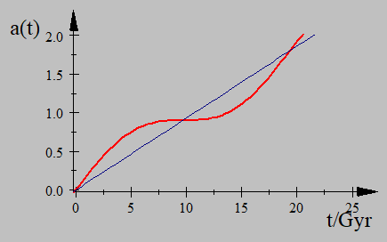
Figure 1: Shows the general features of the time evolution of the scale factor $a(t)$, as depicted by the model. The net expansion (red) which is a combination of two independent influences (basic-space and free matter-energy) is shown as an oscillatory curve about the linear (equilibrium) expansion rate of basic-space. Here we have used $\tau_{\frac{1}{2}}=9.69Gyr$ as the working cosmic half period. Note: $a_{0}\ =1$ at $t=13.76Gyr$.

Figure 2 shows the evolution of the Hubble parameter (red curve) of Eq. 5.9b based on $\tau_{\frac{1}{2}}=9.69$ $Gyr$. The curve oscillates about the would-be equilibrium (or coasting) case (blue hyperbola). Note that here the minimum value of the expansion rate first occurs at same time $\tau_{\frac{1}{2}}=9.69$ $Gyr$ when also (in Figure 1) the general $a(t)\$curve crosses the equilibrium path-line$\ a_{s}=\upsilon^{\ast}t$. Thus, it is at $\tau_{\frac{1}{2}}=9.69$ $Gyr$ the Universe first  virtually comes closest to a halt and also when the current cosmic acceleration commences.

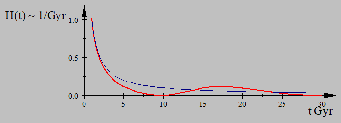
Figure 2: The time evolution of the Hubble parameter $H(t)\$(red curve). The curve is a periodic oscillation, period, about the would-be equilibrium evolutionary path of constant expansion. The intersections between the $H(t)$ curve and the $\frac{1}{t}$ hyperbola identify the ”synchronous points” where $H(t)t=1\$(see discussion below).

6.1.1 The dimensionless age synchronicity problem: why is $H_{0}t_{0}\simeq 1$ now$?$

We now discuss the dimensionless age puzzle.

Problem definition: Cosmological observations, including CMB power spectrum, baryon acoustic oscillations (BAO) and type Ia supernovae (SN Ia) apparent magnitude and redshift measurements [10] [37] do indicate that the current dimensionless age of the Universe appears to be close to unity, $H_{0}t_{0}\simeq 1$. To date, this observation has no satisfactory explanation. When this product is exact unity, it implies the average rate of expansion of the Universe over its entire age,$\frac{\Delta a}{\Delta t}=\frac{a}{t}$, is exactly the same as the Universe’s current local rate of expansion $\dot{a}\left(t\right)$. However, given a history of varied cosmic expansion rate, based on different past cosmic phases, such a result appears puzzling. The Synchronicity Problem [10] then arises out of lack of a satisfactory explanation of the suggestion, implied by this result, that we currently live in a special era when the two ratios are virtually equal. A related question is why the observed current cosmic state gives a result [37] so close to, but not exactly, unity either.

Analysis and resolution: In our approach $H\left(t\right)t=1$ has a natural explanation which also leads to a resolution of the Synchronicity Problem. Recall from Eq. 6.1a the scale-factor $a(t)$ evolves as a periodic function about a coasting path $\upsilon^{\ast}t$. Let us define the ”synchronous time” $t=t_{sy}$ as the time, measured from $t=0$, when in general the relation $\left(\frac{\Delta a}{\Delta t}=\frac{a}{t}\right)=\dot{a}\left(t\right)\Longrightarrow H\left(t\right)t=1$ is satisfied. Then at $\ t=t_{sy}$ we have in our case, on use of Eq. 6.1a, that $\frac{\upsilon^{\ast}\left[1+\cos\left(\frac{t_{sy}}{\tilde{\tau}}\right)\right]t_{sy}}{\upsilon^{\ast}\left[t_{sy}+\tilde{\tau}\sin\left(\frac{t_{sy}}{\tilde{\tau}}\right)\right]}=1$. This sets the ”synchronicity” condition in this approach, as

$$\frac{\tilde{\tau}_{\frac{1}{2}}}{t_{sy}}\tan\left(\frac{t_{sy}}{\tilde{\tau}_{\frac{1}{2}}}\right)=1,$$ (6.3)

where, as before, $\tilde{\tau}_{\frac{1}{2}}=\frac{\tau_{\frac{1}{2}}}{\pi}=\frac{\tau}{2\pi}=\tilde{\tau}$ is the reduced half cosmic period. Note that Eq. 6.3 and Eq. 6.2 refer to, closely related but, different scenarios. Eq. 6.3 admits periodic solutions of the form

$$t_{sy-n}=t_{sy-1}+(n-1)\tau_{\frac{1}{2}},$$ (6.4)

with $n=1,2....$. Using the previously calculated value of $\tau=2\tau_{\frac{1}{2}}=19.38$ $Gyr$ (see also Table 3) we find $t_{sy-1}=13.86_{-0.35}^{+0.17}$ $Gyr$. From Eq. 6.4 the next synchronous point at $t=t_{sy-2}$ appears as $t_{sy-2}=23.55\ Gyr$.

Figure 3 demonstrates the synchronicity situation. The synchronous point at $t=t_{sy-1}$ is shown where the (magenta) line from origin is tangent to the $a\left(t\right)$ (red) curve. As can be seen from Figure 3 this point coincidentally happens to fall within the (model independent ) observational limits [35] of the current age of the Universe $12-15$ $Gyr$.

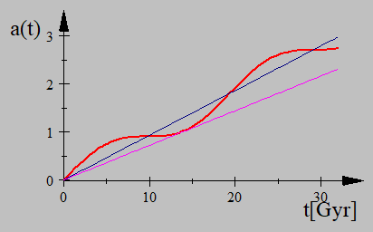
Figure 3: Time evolution of $a(t)$ (similar to Figure 1). The synchronous point appears where the purple line is tangent to the curve where $H\left(t\right)t=1$ (See also Figures 2 3 and 4).

Figures 2 and 4 identify the synchronous points $t_{sy-n}$ much more clearly. In each case, the points appear, respectively, at the intersections of the $H(t)$ curve and the $\frac{1}{t}$ hyperbola, and at the intersection of the $H(t)t$ curve and $f(t)=1$.

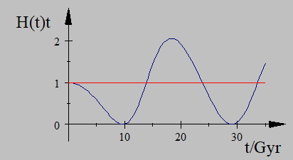
Figure 4: Plot of dimensionless age H(t)t as a function of time t in the model. The Synchronous points appear where this function intersects $f(t)=1\$(blue). They correspond to the points of intersection in Figure 2. Note here that $t=0=t_{sy-0}$ is the first of synchronous points. The Universe is currently approaching the second one.            

Recall we previously estimated the age of the Universe as $t_{0}=13.76\ Gyr$. Inspection of Figures 2 and 3 shows that currently $t_{0}<t_{sy-1}$ and the expansion rate $\dot{a}\left(t\right)\mid_{t_{0}}$ is very close to, but not quite, that at synchronous time, $\ \dot{a}\left(t\right)\mid_{t_{0}}\lesssim\dot{a}\left(t\right)\mid_{t_{sy}}$. According to our current estimate cosmic dynamics will therefore soon become synchronous, at a time from now, of $\left(t_{sy}-t_{0}\right)\simeq\left(13.86-13.76\right)=0.10$ $Gyr$. This is only $\sim 100$ million years from now. As Figures 2, 3- and 4, this event is a once-in-a-half-cosmic-cycle event, $\Delta t=\tau_{\frac{1}{2}}$. Therefore the implication by this analysis is that, according to this model, we currently live in a special era, very close to the first of these special events when the age of the Universe and the Hubble constant become synchronized.

6.2 Density parameters and their evolution

We close this section with a brief discussion regarding the matter-energy fields in the model and their evolution. The net gravitational mass density of all the matter-fields driving the dynamics, in the model, can be inferred from the relation $\frac{\ddot{a}}{a}+\frac{4\pi G}{3}\left(\rho+3p\right)=0$ of Eq. 2.4. Using the solution $a\left(t\right)=a(t)=\upsilon^{\ast}\left[t+\tilde{\tau}\sin\frac{t}{\tilde{\tau}}\right]$ from Eq. 6.1a we find on denoting, here, $\rho+3p=\Delta$, that the net gravitational mass density evolves as

$$\Delta=\frac{3}{4\pi G}\left[\frac{\frac{t}{\tilde{\tau}}\sin\frac{t}{\tilde{\tau}}+\sin^{2}\frac{t}{\tilde{\tau}}}{a^{2}}\right].$$ (6.5)

We note that this is made up of two fields, referred to here as $\Delta_{++}$ and $\Delta_{+-}$with different evolutionary characteristics, such that $\Delta=\Delta_{++}+\Delta_{+-}$, with

$$\Delta_{++}=\frac{3}{4\pi G}\left[\frac{\sin^{2}\frac{t}{\tilde{\tau}}}{a^{2}}\right],$$ (6.6)

and

$$\Delta_{+-}=\frac{3}{4\pi G}\left[\frac{\frac{t}{\tilde{\tau}}\sin\frac{t}{\tilde{\tau}}}{a^{2}}\right].$$ (6.7)

6.2.1 Some effective features of the fields $\Delta_{+-}$ and $\Delta_{++}:\$Cosmic acceleration and flat rotation curves

The gravitational mass density $\Delta$ of Eq. 6.5 represents the net gravitating fields in the model. As Eqs. 6.6 and 6.7 indicate $\Delta$ is made up of two kinds of fields $\Delta_{++}$ and $\Delta_{+-}$ which are functionally different. Below we highlight on some of these characteristics.

Features of $\Delta_{+-}$ as dark energy: The field $\Delta_{+-}$ is an odd function and changes its gravitational charge signature periodically, being currently negative. We will take $\Delta_{+-}$to contribute the net negative pressure component of dark energy which provides the acceleration of the universe in the model. To justify this assumption we evaluate $\Delta_{+-}$ in relation to $\Delta_{++}$, in section 6.2.2 below, and compare the results with observations.

Features of $\Delta_{++}$ as matter/dark matter: The field $\Delta_{++}$ is an even function with positive-definite gravitational charge signature, reminiscent of regular or dark matter. Because in this model, fields are only distinguished by their net gravitational charge, $\Delta_{++}$ represents all matter including dark matter, baryonic matter, radiation and neutrinos (and excludes negative pressure included in $\Delta_{+-}$). For a realistic model consistent with observations, one expects $\Delta_{++}$ to be dominated by a dark energy density $\rho_{d}$. To test this we make the reasonable assumption, based on its positive gravitational signature, that during structure formation the field $\Delta_{++}$ coalesces into galaxies enveloped, and dominated, by dark matter haloes. Considering $M\left(R\right)$ as the mass of such a halo enclosed by a distance $R$ from the origin, where $R>R_{0\text{ }}$($R_{0\text{ }}$ being the extent of the baryonic matter in the galaxy, of mass $M_{0}$), then along $R>R_{0\text{ }}$, the orbital velocities $v$ of the galaxy satellites can be obtained from their centripetal and gravitational accelerations relation, $\frac{v^{2}}{R}=\frac{GM}{R^{2}}$. In our case $\frac{GM}{R^{2}}\sim\frac{4}{3}\pi GR\Delta_{++}$. Given (see Eq. 6.6) that $\Delta_{++}\propto\frac{\sin^{2}\frac{t}{\tilde{\tau}}}{a^{2}}\propto\frac{\sin^{2}\frac{t}{\tilde{\tau}}}{R^{2}}$, and noting that $\sin^{2}\frac{t}{\tilde{\tau}}$ is a slowly varying function (with a long period $\tau\approx 19.38Gyr$), we see that for distances of few tens $kpcs$ usually associated with such halos [41] $v$ is constant. It follows then that the model produces fields identifiable as dark matter and whose halos have the physical structure to generate flat rotation curves in galaxies. Such flat rotation curves are consistent with observations [42] [43] [44]. We therefore consider this a noteworthy result of the model, whose detailed analysis and discussion will follow in an upcoming work.

6.2.2 Comparison with observations

It is reasonable to ask how the above gravitational mass density results do relate to current observations of an accelerating Universe. In principle, one should relate the strength (density) of the negative pressure causing the acceleration of space to the available inertia from the matter-energy density. In our case, the key quantities to compare with observations are the net accelerating field density $\Delta_{+-}$ and the source of inertia to be accelerated $\Delta_{++}$, and the comparison can sufficiently be expressed in the form $\frac{\Delta+-}{\Delta++}$.

In the $\Lambda CDM$ model, cosmic acceleration is assumed to be driven by a dark energy with an energy density $\rho_{de}$ and pressure $p_{de}$ which can be represented as an energy momentum tensor of a perfect fluid $T^{\mu\nu}=diag(\rho_{de},p_{de},\rho_{pde},p_{de})$. Its contribution to cosmic dynamics can be inferred from Eq. 2.4 as $\frac{\ddot{a}}{a}+\frac{4\pi G}{3}\left(\rho_{de}+3p_{de}\right)=0$. In particular, in $\Lambda CDM$ the dark energy density $\rho_{de}$ is assumed constant in time, satisfying an equation of state $p_{de}=-\rho_{de}$. It follows that, for a field with an energy density $\rho_{de}$, the driver of cosmic acceleration in $\Lambda CDM$ is a net negative pressure equivalent to $\rho_{de}-3\rho_{de}=-2\rho_{de}$. Therefore, from observations the ratio of the source of the acceleration to the source of inertia $\rho_{m}$ would be $\frac{\left|-2\rho_{de}\right|}{\rho_{m}}$. This result $\frac{\left|-2\rho_{de}\right|}{\rho_{m}}$, just like $\frac{\left|\Delta_{++}\right|}{\Delta_{+-}}$, is model-independent. In our present case, using Eq. 6.6 and Eq. 6.7 and our previously determined values of $t_{0}=13.76Gyrs$ and $\tau\simeq 19.38Gyrs$ we find $\frac{\left|\Delta+-\right|}{\Delta++}=4.\,605\,2$. Below, we show that this result is consistent with recent observations [6] (usually represented differently).

Traditionally, the results giving the ratio of the source of the acceleration to the inertia to accelerate is given, instead, in terms of the dark energy density $\rho_{de}$ and the matter-energy density $\rho_{m}$ (or more precisely in terms of their weighted parameters $\Omega_{de}$ and $\Omega_{m}$). This follows the observation that in $\Lambda CDM$, the driving pressure and the dark energy density are connected by the equation of state $p_{de}=-\rho_{de}$, making it more intuitively easier to compare the densities, instead. While valid for $\Lambda CDM$, such presentation is, clearly, model-dependent.

For easier, more transparent, verification we will now present the above result ($\frac{\left|\Delta+-\right|}{\Delta++}=4.\,605\,2$) using the (now common $\Lambda CDM$ ) approach of the density $\rho_{de}$ instead of the driving pressure $-2\rho_{de}$. To do this, denote by $\left|\Delta_{\frac{1}{2}\left(+-\right)}\right|=\frac{1}{2}\left|\Delta_{+-}\right|$ the analogue of $\rho_{de}=\frac{1}{2}\left|2p_{de}\right|$ in $\Lambda CDM$. Then in our model, the analogue of the net density in $\Lambda CDM$ would be $\left|\Delta_{\frac{1}{2}\left(+-\right)}\right|+\Delta_{++}$ It follows that the percentage contributions to this by the dark energy, and by matter, in our model at any time $t$ can be respectively computed from $\frac{\left|\Delta_{\frac{1}{2}\left(+-\right)}\right|}{\left|\Delta_{\frac{1}{2}\left(+-\right)}\right|+\Delta_{++}}$ and $\frac{\Delta_{++}}{\left|\Delta_{\frac{1}{2}\left(+-\right)}\right|+\Delta_{++}}$. In particular one finds the current values to be $\Omega_{de}=\left[\frac{\left|\Delta_{\frac{1}{2}\left(+-\right)}\right|}{\left|\Delta_{\frac{1}{2}\left(+-\right)}\right|+\Delta_{++}}\right]_{t=t_{0}}=0.697\,21$ and $\Omega_{m}=\left[\frac{\Delta_{++}}{\left|\Delta_{\frac{1}{2}\left(+-\right)}\right|+\Delta_{++}}\right]_{t=t_{0}}=0.302\,79$, where we used our results of $t_{0}=13.76Gyr$ and $\tau=19.38Gyr$.

Therefore summarizing, we have that taking the field $\Delta_{+-}$ in Eq. 6.6 to constitute the net driver of the acceleration (with $\left|\Delta_{\frac{1}{2}\left(+-\right)}\right|$ as its effective density corresponding to $\rho_{de}$ in $\Lambda CDM$) and taking the field $\Delta_{++}$ in Eq. 6.7 to constitute the mass-energy density (analogous to $\rho_{m}$) we have shown that, in this model, the analogous dark energy density contributes $\Omega_{de}=69.7\%$ while the entire matter sector contributes $\Omega_{m}=30.3\%$. These results are consistent with the recent observations [6].

6.3 Summary of results

Summarizing, we have in this section applied the current approach to discuss evolutionary features of the standard cosmological parameters and calculated their current values. Based on the estimated [3] acceleration commencement look-back time $t_{ac}$, we found from a range of choices that $t_{ac}=4.07\pm 0.05$ $Gyr$ gave estimates most consistent with observations for all the parameters. Using this value of $t_{ac}$ we estimated the age of the Universe $t_{0}$, the Hubble constant $H_{0}$. The results are consistent with the latest observations.[38][6][39][40]. The model also generates two fields $\Delta_{+-}$and $\Delta_{++}$ which we identified as the net pressure (component) of dark energy and net matter/dark matter density component. We have showed the two fields have the desirable characteristics. In particular $\Delta_{+-}$ can accelerate the universe, while $\Delta_{++}$ can constitute lumpy matter. The latter also provides dark matter halos with the correct density profile that can produce the observed flat rotation curves [42] [43] [44].. We have, futher, showed that the two fields $\Delta_{+-}$and $\Delta_{++}$ give the observed respective relative percentages of dark energy and of matter densities, in the universe [6]. Finally, in the process, we have also introduced some new parameters including the cosmic period $\tau$, and the synchronous time $t_{sy}$ and addressed the synchronicity problem. Table 2, below, summarizes our estimates of cosmological parameters, in the model.

$$Table2 :Summary\ of\text{ }model\prime s\ calculated\ best\ estimates\ of\ cosmological\text{ }parameters.$$

7 Concluding remarks

In this work we have presented a framework to discuss dynamics of a universe with self-regulating features. The approach builds on the Friedman model by introducing two ingredients. First, that basic-space is endowed with a physical structure and this makes it one of the active drivers of the dynamics of this universe, and second that matter-energy emerges as a perturbation to the structure and to the dynamics of this universe. The underlying idea that basic-space has structure leads to a flat geometry with a time-linear expanding space as the ideally unperturbed dynamic equilibrium state. We have described these contributions of basic-space to the dynamics of the modeled universe. Later we added those contributions of free matter-energy, as perturbations. The two ingredients are linked through a proposal referred to as the Dynamic Equilibrium Protection Proposal (DEPP). According to DEPP cosmic dynamics always seeks stability against perturbations of its dynamic equilibrium state. We combined the two contributions into one framework to describe the over-all dynamics. It describes a universe that oscillates periodically about a time-linearly, monotonically expanding path. The model isolates two density fields $\Delta_{++}$ and $\Delta_{+-}$ driving the dynamics

We have compared the features and characteristics of the modeled universe with the observed physical Universe. We find the former reproduces very well the general evolutionary profile of the observed Universe from the early big bang phase through radiation and structure formation phases to the current acceleration. The model is shown to have neither a horizon problem nor a flatness problem. Its initial phase acceleration ends into a big bang and matter creation. Similarly, the second acceleration, after structure formation, begins predictably and will end predictably. Further, subject only to observational constraints of when the current cosmic acceleration initiated, the model is able to reproduce the standard current values of the cosmological parameters, accurately, including the age, $t_{0}$, the Hubble $H_{0}$ and the density parameters of dark energy $\Omega_{de}$ and that of gravitating matter-energy fields $\Omega_{m}$ to a high accuracy consistent with recent observations. The dark matter produced in the model has a density profile that facilitates flat rotation curves in galaxy halos, consistent with observations.

We have demonstrated the model can address some standing puzzles. As an example we have discussed the origin of the dimensionless age/synchronicity problem and addressed it, in the process fixing the various times in future when cosmic dynamics will satisfy $Ht=1$. With regard to testability, the model predicts features that make it testable and falsifiable. For example according to the model the beginning of cosmic acceleration $t_{ac}\sim 4Gyr$ ago, also marks both the minimum expansion rate $\dot{a}_{\min}$ (see Figures 1 and 2) and the minimum of dark matter-energy density content $\Delta_{++}$ (see Eqs. 6.6 and 6.7). Therefore the temporal region of about $2-3Gyr$ centered at this point  constitutes a phase referred to here as the ”Cosmic Valley”, with special testable features. In the Cosmic Valley: 1) Expansion rate tests such as Type 1A supernovae should register lower than expected radial recession velocities of galaxies; 2) Galaxies observed in this region should mostly be compact with little or no dark matter halos. 3) The predicted primordial non-inflationary accelerated expansion of the model may favor earlier than expected formation of structure. Finally, it is expected that more tests, including CMB based, nucleosynthesis and structure formation will improve the model.

Appendix1

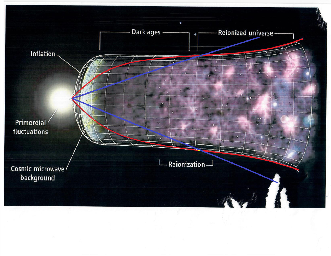
Figure 5: A diagramatic sketch of cosmic evolution: based on lambdaCDM model (Courtesy of NASA/WMAP Science Team). Superimposed on it is our model (in red) snaking about a (blue not on scale) coasting path.

References

- [1] Perlmutter, S., Aldering, G., Goldhaber, G., et al.; Measurements of and from 42 High-Redshift Supernovae, ApJ, 517, 565 (1999).
- [2] Riess, A. G., Filippenko, A. V., Challis, P., et al.; Observational Evidence from Supernovae for an Accelerating Universe and a Cosmological Constant1998, AJ, 116, 1009.
- [3] J. A. Frieman, M. S. Turner, D. Huterer, Dark Energy and the Accelerating Universe, Ann. Rev. of AA 46 (1): 385–432 (2008)
- [4] J. S. Bullock and M. Boylan-Kolchin, Small-Scale Challenges to the CDM Paradigm, Ann. Rev. AA 55 343-387 (2017).
- [5] A. Guth, Inflationary universe: A possible solution to the horizon and flatness problems, Phys. Rev. D 23, 347 (1981).
- [6] N. Aghanim et al, Planck Collaboration, Planck 2018 results. VI. Cosmological parameters, arXiv:1807.06209 [astro-ph.CO].
- [7] A. Benoit-Levy and G. Chardin, Introducing the Dirac-Milne universe, AA 537 A78 (2012).
- [8] N. Menci, et al, Morpheus Reveals Distant Disk Galaxy Morphologies with JWST: The First AI/ML Analysis of JWST Images, arXiv:2208.1147v1 [astro-ph CO] 24 Aug. 2022
- [9] K. Suess, et al., Rest-frame near-infrared sizes of galaxies at cosmic noon: objects in JWST’s mirror are smaller than they appeared, arXiv.2207:10655v2 [astro/ph.GA] 20 Sep 2022
- [10] A. Avelino and R. P. Kirshner, The dimensionless age of the Universe: A riddle for our time, ApJ. 828 1 (2016).
- [11] P. J. Steinhardt, N. Turok, Endless Universe. New York: Doubleday. ISBN 978-0-385-50964-0 (2007).
- [12] A. Ajja and P. steinhardt, Bouncing Cosmology made simple, arXiv:1803.01961 [astro-ph.CO].
- [13] V. G. Gurzadyan, R. Penrose, On CCC-predicted concentric low-variance circles in the CMB sky, arXiv:1302.5162 [astro-ph.CO].
- [14] K. Arun, S. B. Gudennarar, C. Sivaram, Dark Matter, Dark Energy, and Alternate Models: A Review, Adv. Space Res., 60 1,166-186 (2017).
- [15] A. Einstein, Peuss. Akad. Wiss. Berlin, Sitzber. 778 (1915)
- [16] S. Weinberg, Gravitation and Cosmology, John Wiley & Sons, NY, (1972).
- [17] E. Hubble; A relation between distance and radial velocity among extra-galactic nebulae, Proc. Nat. Acad. Sc., 15 3: March 15, (1929).
- [18] N. Cohen, Gravity’s Lens: Views of the New Cosmology, Wiley and Sons, 1988
- [19] B. P. Abbott; et al. (LIGO Scientific Collaboration and Virgo Collaboration (2016)), Observation of Gravitational Waves from a Binary Black Hole Merger, Phys. Rev. Lett. 116 (6): 061102.
- [20] L. Smolin, Atoms of Space and Time-Scientific American, February 2006
- [21] C. Rovelli, Quantum Gravity, CUP, Cambridge (2004); Quantum Gravity, Scholarpedia 3 (5): 7117 (2008)
- [22] D. N. Spergel, et al, Wilkinson Microwave Anisotropy Probe (WMAP) Three Year Observations: Implications for CosmologyAA Supl. Series 170 (2) 337-408 (2007); arXiv: astro-ph/0603449.
- [23] E. A. Milne, Relativity, Gravitation and World Structure, Oxford Univ. Press, 1935.
- [24] E. W. Kolb, A coasting cosmology. Astrophys. J. 344, 543–550 (1989).
- [25] F. Melia, A. S. H. Shevchuk, The Rh=ct universe Mon.Not.Roy.Astron. Soc. 419 2579-2586 (2012).
- [26] M. V. John,.Realistic coasting cosmology from the Milne model, arXiv:1610.09885
- [27] J. Casado, Linear expansion models vs. standard cosmologies: a critical and historical overview, Astrophys. Space Sci. 365 16 (2020).
- [28] S. Pan, J. Hiro, A. Paliathanasisde, R. J.. Slagter, Evolution and dynamics of a matter creation model, MNRAS, 460 1445 (2016).
- [29] A. Palianthanasis, J. D. Barrow and S. Pan, 4 May 2017.Cosmological solutions with gravitational particle production and nonzero curvature, Phys. Rev. D 95, 103516 (2017); arXiv:1610.02893 [gr-qc]
- [30] H. Bondi, Negative Mass in General Relativity, Rev. Mod. Phys. 29 423, (1957).
- [31] F. Hole, A Covariant Formulation of the Law of Creation of Matter, .MNRAS, 120 3 (1960).
- [32] I. Prigoggine and J. Gahineau, E. Gunzig, P. Nardone, Thermodynamics and Cosmology, Gen. Rel. and Grav. 21 8 (1989).
- [33] NASA/WMAP Science Team (6 June 2011). ”Cosmology: The Study of the Universe”.
- [34] R. A. Alpher, H. A., Bethe, G. Gamov, The Origin of Chemical Elements, Phys. Rev.73, 803–804 (1948)
- [35] L. Kofman, A. Linde, A. Starobinsky, Reheating after Inflation, arXiv:hep-th/9405187 (hep-th).
- [36] M. R. Mbonye, Cosmology with interacting dark energy, Mod. Phy. Lett. A 19 2 (2002).
- [37] J. Tonry, B. et al, Cosmological results from high-z supernovae, ApJ. 594, 1 (2003).
- [38] L. M. Kraus and B. Chaboyer, Age estimates of globular clusters in the Milky Way: constraints on cosmology, Science 299 65 (2003).
- [39] W. L. Freedman et al, Measurements of the Hubble Constant: Tensions in Perspective, Xiv:2106.15656v1 [astro-ph.CO]
- [40] N. Khetan, L. Izzo, M. Branchesi, et al, A new measurement of the Hubble constant using Type Ia supernovae calibrated with surface brightness fluctuations, AA 647 A72 (2021).
- [41] P. M. Drew et al, Evidence of a Flat Outer Rotation Curve in a Star-bursting Disk Galaxy at z= 1.6, ApJ 869 58 (2018).
- [42] H. Mo, F. van den Bosch and S. White, Galaxy Formation and Evolution. Camb. Univ. Press. (2010) ISBN 978-0-521-85793-2.
- [43] G. Sharma, O. Salucci, G. Van de Ven, Flat rotation curves of z1 forming galaxies MNRAS, 503 2 (2021)
- [44] R. H. Wechsler and J. L. Tinker, The Connection Between Galaxies and Their Dark Matter Halos, Ann Rev.AA 56 1 2018.