Long time behavior of solutions to the generalized Boussinesq equation in Sobolev spaces

Abstract

In this paper, we study the generalized Boussinesq equation to model the water wave problem with surface tension. First we investigate the initial value problem in the Sobolev spaces. We derive some conditions under which the solutions of this equation are global or blow-up in time, and next we extend our results to the Bessel potential spaces. The asymptotic behavior of the solutions is also determined. The non-existence of solitary waves for some parameters are proved using Pohozaev type identities. We generate solitary wave solutions of generalized Boussinesq equation using the Petviashvili iteration method numerically. In order to investigate time evolution of solutions to the generalized Boussinesq equation, we propose the Fourier pseudo-spectral numerical method. After studying the time evolution of the single solitary wave, we focus on the gap interval where neither a global existence nor a blow-up result has been established theoretically. Our numerical results successfully fill the gaps left by the theoretical ones.

1 Introduction

In this paper, we study the generalized Boussinesq (gBq) equation

$$\begin{cases}u_{tt}={\big{(}u-\alpha u_{xx}+u_{tt}-\kappa u_{xxtt}+f(u)\big{)}}_{xx},\\ u(x,0)=u_{0}(x),\quad u_{t}(x,0)=u_{1}(x),\quad\alpha,\kappa\geq 0.\end{cases}$$ (1.1)

This equation was proposed by Schneider and Eugene [23] to model the water wave problem with surface tension when $f(u)=u^{2}$. The solution $u(x,t)$ of (1.1) can be interpreted the vertical velocity component on the top surface of an irrotational, incompressible fluid in a domain. Equation (1.1) can also be derived from the two dimensional water wave problem. In a degenerate case (with Bond number $T=\frac{1}{3}$, a dimensionless parameter proportional to the surface tension), it was shown in [23] that the long wave limit can be described approximately by two decoupled Kawahara equations. In was also proved that the (improved) Boussinesq equation,

$$u_{tt}={(u+u_{tt}+u^{2})}_{xx},$$ (1.2)

is useful in the case of zero surface tension [22]. Equation (1.2) is formally equivalent to the most well known and classical Boussinesq equation

$$u_{tt}={(u\pm u_{xx}+u^{2})}_{xx},$$ (1.3)

which is also (from a formal point of view) valid for unidirectional wave propagation in the water wave problem [17]. Equation (1.3) was first derived in [2] (rediscovered later by Keulegan and Patterson [11]) in investigating the bidirectional propagation of small amplitude and long wavelength capillary-gravity waves on the surface of shallow water. Since the linear part of (1.3) with $+u_{xx}$ term contains the backward heat operator $\partial_{t}+\partial_{x}^{2}$, it is ill-posed. This does not occur with $-u_{xx}$ term, but in this case cannot be proved as a physical model of water waves as the original Boussinesq equation. In order to compensate for this situation, and related to (1.1), the following generalized Boussinesq equation was derived in [4] (see also [8] and references therein):

$$u_{tt}={(u\pm u_{xx}+u_{xxxx}+u^{2})}_{xx}.$$ (1.4)

Rosenau [20] was proposed the higher order Boussinesq (HBq) equation

$$u_{tt}=(u+\eta_{1}u_{tt}-\eta_{2}u_{xxtt}+(f(u))_{xx}$$ (1.5)

where $\eta_{1}$ and $\eta_{2}$ are real positive constants in order to include the higher order effects of dispersion. A more recent derivation of the HBq equation is given in [7] to model the bi-directional propagation of longitudinal waves in an infinite, nonlocally elastic medium.

Regarding the existence of local/global solutions of the initial value problem associated with (1.3), Bona and Sachs used Kato’s theory to show the local well-posedness of smooth solutions. This result was extended to $H^{1}$ in [28]. For the nonlinearity $f(u)=-|u|^{p}u$, it was shown in [14] the existence of $L^{2}$- and $H^{1}$-solutions of (1.1). It also proved in [14] that these solutions, with small initial data, are global in $H^{1}$ if $0<p<4$. The existence of finite-time blow-up of solutions, decay of small solutions, and strong instability of a solitary wave with small speed of propagation for the Cauchy problem of the Boussinesq equation were investigated in [16].

In this paper, we study the initial value problem (1.1). The well-posedness for (1.1) was shown in [29] by using the contraction mapping principle. Here we improved the results of [29] to the lower Sobolev indices (See Theorem 2.2) in Section 2. Wang and Xu in [29] also obtained some conditions under which solutions of problem (1.1) are global or blow up by applying the potential well approach. These results rely on the potential well depth $d$ and constructing two stable and unstable submanifolds of $H^{2}$. The value $d$ is determined variationally in terms of stationary solution of (1.1), that is the unique positive solution of

$$0=Q_{0}-\alpha Q_{0}^{\prime\prime}+\beta Q_{0}^{p+1},\qquad\beta<0.$$

Our next aim in this paper is to study the time-decay behavior of solutions of (1.1). First we use the properties of the group associated to the linear part of (1.1) and extend our local well-posedness result to the Bessel potential spaces $H^{s,q}(\mathbb{R})$ in Section 3. In Section 4, we present two equivalent forms of equation (1.1) and use again decay properties of the linear part of (1.1) and obtain some time decay estimates of solution in $L^{\infty}$ and $H^{s}$ spaces.

We also study the existence of nonstationary solitary waves of (1.1). Contrary to the stationary case, we observe that the coefficient of $\beta$ should be positive to guarantee the existence of solitary waves. We refer reader to Section 5 to see some non-existence results. To the best of our knowledge, the analytical solitary wave solution of (1.1) is unknown, we use the Petviashvili’s iteration method to generate the solitary wave solution numerically in Section 5.

A numerical method combining a Fourier pseudo-spectral method in space and a Runge Kutta method in time for time evolution of solutions of the gBq equation is proposed in Section 6. To the best of our knowledge, there is no numerical study for gBq equation although there have been a large amount of works in the literature to solve the equations (1.2)-(1.5) (see [1, 3, 10, 24, 26, 27] and references therein). The time evolution of the generated solitary waves obtained by the Petviashvili’s iteration method is studied in Section 6. There is a gap interval where neither a global existence nor a blow-up result has been established analytically in Section 2. After we confirm the analytical results obtained for global existence and blow-up numerically given in Section 2, we present some numerical results for the behavior of solutions corresponding to the gap interval. We obtain a threshold value. When the initial amplitude is below this threshold, the solution exists globally. If the initial amplitude exceeds this threshold, then the solution blows-up in finite time.

In the throughout of this paper, we assume that $f\in C(\mathbb{R})$ such that $|f(u)|\leq C|u|^{p+1}$ and $C\geq 0$, and $\|u\|_{s}$ stands by the norm of $u$ in the Soblev space $H^{s}(\mathbb{R})$.

2 Well-posedness

In this section, we study the well-posedness of initial value problem (1.1). To do so, first, similar to the method in [8], by using a Fourier transform and the Duhamel principle, the solution of problem (1.1) can be written as follows:

$$u(x,t)=\mathbb{A}(u)=\partial_{t}S(t)u_{0}(x)+S(t)u_{1}(x)+\int_{0}^{t}S(t)\mathcal{L}_{R}^{-1}\partial_{x}^{2}f(u){\;\rm d}\tau,$$ (2.1)

where $\mathcal{L}_{R}=I-\partial_{x}^{2}+\kappa\partial_{x}^{4}$ and

$$\partial_{t}S(t)=\cos\left(\frac{t|\xi|\sqrt{1+\alpha\xi^{2}}}{\sqrt{1+\xi^{2}+\kappa\xi^{4}}}\right),\qquad S(t)=\sin\left(\frac{t|\xi|\sqrt{1+\alpha\xi^{2}}}{\sqrt{1+\xi^{2}+\kappa\xi^{4}}}\right)\frac{\sqrt{1+\xi^{2}+\kappa\xi^{4}}}{|\xi|\sqrt{1+\alpha\xi^{2}}}.$$

Remark 2.1.

Notice that $\mathcal{L}_{R}^{-1}f=K\ast f$, where

$$K(x)=\kappa\pi\left\{\begin{array}[]{lll}\frac{1}{\lambda_{2}^{2}-\lambda_{1}^{2}}\left(\frac{1}{\lambda_{1}}{\rm e}^{-\lambda_{1}|x|}-\frac{1}{\lambda_{2}}{\rm e}^{-\lambda_{2}|x|}\right),&&4\kappa<1,\\ \\ \frac{\kappa^{\frac{3}{4}}}{2}\left(1+\kappa^{-\frac{1}{4}}|x|\right)\;{\rm e}^{-\kappa^{-\frac{1}{4}}|x|},&&4\kappa=1,\\ \\ \frac{e^{-\sigma|x|}}{2\sigma\omega(\sigma^{2}+\omega^{2})}\left(\omega\cos(\omega x)+\sigma\sin(\omega|x|)\right),&&4\kappa>1,\end{array}\right.$$ (2.2)

and

$$\begin{split}&\lambda_{1}=\sqrt{\frac{1}{2\kappa}\left(1-\sqrt{1-4\kappa}\right)}\qquad\lambda_{2}=\sqrt{\frac{1}{2\kappa}\left(1+\sqrt{1-4\kappa}\right)}\\ &\sigma=\frac{1}{2}\sqrt{\frac{2}{\sqrt{\kappa}}+\frac{1}{\kappa}}\qquad\omega=\frac{1}{2}\sqrt{\frac{2}{\sqrt{\kappa}}-\frac{1}{\kappa}}.\end{split}$$ (2.3)

It is clear that $K$ is real-valued, even, continuous function in $\mathbb{R}$. Moreover, $K$ is smooth at $\mathbb{R}\setminus\{0\}$ and all its derivatives decay exponentially. Furthermore, $K^{(n)}\in L^{q}(\mathbb{R})$ for any $1\leq q\leq\infty$ and $n\in\mathbb{N}$.

By the arguments in [29], we can obtain the following lemmas.

Lemma 2.1.

The following inequalities hold for all $\varphi\in H^{s}(\mathbb{R})$ and $\psi\in H^{s-2}(\mathbb{R})$:

1. $\|\partial_{t}S(t)\varphi\|_{s}\leq\|\varphi\|_{s}$,

2. $\|S(t)\varphi\|_{s}\leq 2(1+t)\|\varphi\|_{s}$,

3. $\|\partial_{tt}S(t)\varphi\|_{s}\leq\sqrt{2(1+t)}\|\varphi\|_{s}$,

4. $\|\mathcal{L}_{R}^{-1}S(t)\partial_{x}^{2}\psi\|_{s}\leq\sqrt{2}\|\psi\|_{s-2}$,

5. $\|\mathcal{L}_{R}^{-1}\partial_{t}\partial_{x}^{2}S(t)\psi\|_{s}\leq\|\psi\|_{s-2}$.

Lemma 2.2.

Let $f\in C^{m}(\mathbb{R})$, where $m\geq 0$ is an integer. Then the following statements hold.

1. If $0\leq s\leq m$ and $u\in H^{s}(\mathbb{R})\cap L^{\infty}(\mathbb{R})$, then $f(u)\in H^{s}(\mathbb{R})$ and $\|f(u)\|_{s}\leq C(\|u\|_{L^{\infty}(\mathbb{R})})\|u\|_{s}$.

2. If $\leq s\leq m$ and $u,v\in H^{s}(\mathbb{R})\cap L^{\infty}(\mathbb{R})$, then $\|f(u)-f(v)\|_{s}\leq C(\|u\|_{L^{\infty}(\mathbb{R})},\|v\|_{L^{\infty}(\mathbb{R})})\|u-v\|_{s}$.

Now we define the function space $X(T)=C^{1}(0,T;H^{s}(\mathbb{R}))$ equipped with the norm

$$\|u\|_{X(T)}=\sup_{t\in[0,T]}(\|u(t)\|_{s}+\|u_{t}(t)\|_{s}).$$

Using the Sobolev embedding and the arguments in [29] one can prove the following result.

Theorem 2.1.

Let $f\in C^{m}$ with $m\geq s$. If $u_{0},u_{1}\in{H^{s}(\mathbb{R})}$, then there exist $T>0$ and a unique solution $u\in C^{1}([0,T],{H^{s}(\mathbb{R})})$ of (1.1).

In the case $p\in\mathbb{N}$, we can extend the above result to the lower Sobolev indices.

Theorem 2.2.

Let $u_{0},u_{1}\in H^{s}(\mathbb{R})$ and $p\in\mathbb{N}$. Assume that $s>\frac{p-1}{2(p+1)}$ if $p>1$ and $s\geq 0$ if $p=1$. Then there exists $T>0$ and a unique solution $u\in C^{1}(0,T;H^{s}(\mathbb{R}))$ such that $u(0)=u_{0}$ and $u_{t}(0)=u_{1}$. Moreover, if $T<+\infty$ is the maximal existence time of $u$, then

$$\sup_{t\in[0,T]}(\|u(t)\|_{s}+\|u_{t}(t)\|_{s})=+\infty.$$

Furthermore, we have $u_{tt}\in C(0,T;H^{s}(\mathbb{R}))$. In addition, if $(-\partial_{x}^{2})^{-\frac{1}{2}}u_{1}\in L^{2}(\mathbb{R})$, then $(-\partial_{x}^{2})^{-\frac{1}{2}}u_{t}\in C^{1}(0,T;L^{2}(\mathbb{R}))$.

Proof.

It is shown that the right hand side of (2.1) defined is a contraction mapping $A$ of $C(0,T;B)$ for some $T>0$, where $B$ is a closed ball in $X(T)$. Indeed, since $S$ and $\partial_{t}S$ are both bounded on $H^{s}(\mathbb{R})$, then it is enough to study the nonlinear part of (2.1).

Note that when $p=1$, then $\langle\xi\rangle^{s}|\widehat{f(u)}|\leq(\langle\xi\rangle^{s}|\hat{u}|)\ast(\langle\xi\rangle^{s}|\hat{u}|)\leq\|u\|_{s}^{2}$, where $\langle\xi\rangle=1+|\xi|$. If $p>1$, then we get from the Young inequality that

$$\begin{split}\langle\xi\rangle^{s_{1}}|\widehat{f(u)}|&\leq(\langle\xi\rangle^{s_{1}}|\hat{u}|)\ast\cdots\ast(\langle\xi\rangle^{s_{1}}|\hat{u}|)\\ &\leq\left\|\langle\xi\rangle^{s_{1}}|\hat{u}|\right\|_{L^{(p+1)/p}(\mathbb{R})}^{p+1}\leq\|u\|_{s}^{p+1}\left(\int_{\mathbb{R}}\langle\xi\rangle^{\frac{2(p+1)(s_{1}-s)}{p-1}}{\;\rm d}x\right)^{\frac{p-1}{2}}\\ &\lesssim\|u\|_{s}^{p+1}\end{split}$$ (2.4)

provided $s>s_{1}+\frac{p-1}{2(p+1)}$. We have from the above inequalities that

$$\begin{split}\|\partial_{x}^{2}\mathcal{L}_{R}^{-1}f(u)\|_{s}^{2}&=\int_{\mathbb{R}}\frac{\xi^{4}\langle\xi\rangle^{2s}}{(1+\xi^{2}+\kappa\xi^{4})^{2}}|\widehat{f(u)}|^{2}{\;\rm d}\xi\\ &\lesssim\int_{\mathbb{R}}\langle\xi\rangle^{2s-4}|\widehat{f(u)}|^{2}{\;\rm d}\xi\\ &\lesssim\|u\|_{s}^{2(p+1)}\int_{\mathbb{R}}\langle\xi\rangle^{2s-4-2s_{1}}{\;\rm d}x\\ &\lesssim\|u\|_{s}^{2(p+1)},\end{split}$$

for any $s>\frac{p-1}{2(p+1)}$ if $p>1$, and $s\geq 0$ if $p=1$.

Next, we have from (1.1) that

$$\hat{u}_{tt}=-\frac{\xi^{2}(1+\alpha\xi^{2})}{1+\xi^{2}+\kappa\xi^{4}}\hat{u}+\frac{\xi^{2}}{1+\xi^{2}+\kappa\xi^{4}}\widehat{f(u)}.$$ (2.5)

Then,

$$\|u_{tt}\|_{s}=\|\hat{u}_{tt}\|_{s}\lesssim\|u\|_{s}+\|u\|_{s}^{p+1}\leq C(t)$$

for any $t\in(0,T)$. On the other hand, we get from

$$\|u_{tt}(t+\Delta t)-u_{tt}(t)\|_{s}=\|\hat{u}_{tt}(t+\Delta t)-\hat{u}_{tt}(t)\|_{s}\leq C(T)\|u(t+\Delta t)-u(t)\|_{s}\to 0,\quad\mbox{as}\,\,\Delta t\to 0,$$

that $u_{tt}\in C(0,T;H^{s}(\mathbb{R}))$.

Now, we show that $(-\partial_{x}^{2})^{-\frac{1}{2}}u_{t}\in C^{1}(0,T;L^{2}(\mathbb{R}))$ if $(-\partial_{x}^{2})^{-\frac{1}{2}}u_{1}\in L^{2}(\mathbb{R})$. Similar to above argument, we have from (2.5) and (2.4) that

$$\left\|\frac{|\xi|(1+\alpha\xi^{2})}{1+\xi^{2}+\kappa\xi^{4}}\hat{u}\right\|_{s+1}\lesssim\|u\|_{s}^{2}$$

and

$$\left\|\frac{|\xi|}{1+\xi^{2}+\kappa\xi^{4}}\widehat{f(u)}\right\|_{s+1}^{2}\leq C(\|u\|_{s})\|u\|_{s}^{2}.$$

Analogous the above estimate, we can show that

$$\left\|(-\partial_{x}^{2})^{-\frac{1}{2}}u_{tt}(t+\Delta t)-(-\partial_{x}^{2})^{-\frac{1}{2}}u_{tt}(t)\right\|_{s+1}\to 0\quad\mbox{as}\,\,\Delta t\to 0.$$

So that $(-\partial_{x}^{2})^{-\frac{1}{2}}u_{tt}\in C(0,T;H^{s+1}(\mathbb{R}))$. Now, if $(-\partial_{x}^{2})^{-\frac{1}{2}}u_{1}\in L^{2}(\mathbb{R})$, then we derive from

$$(-\partial_{x}^{2})^{-\frac{1}{2}}u_{t}=(-\partial_{x}^{2})^{-\frac{1}{2}}u_{1}+\int_{0}^{t}(-\partial_{x}^{2})^{-\frac{1}{2}}u_{\tau\tau}{\;\rm d}\tau$$

that $(-\partial_{x}^{2})^{-\frac{1}{2}}u_{t}\in C^{1}(0,T;L^{2}(\mathbb{R}))$. ∎

In order to get more time-regularity of the local solution, we obtain the following result by using Lemma 2.1. The invariant $E$ also shows that the solutions is global in time.

Theorem 2.3.

Let $s\geq 1$ and $u_{0},u_{1}\in H^{s}(\mathbb{R})$ and $(-\partial_{x}^{2})^{-\frac{1}{2}}u_{1}\in H^{s+1}(\mathbb{R})$. Then the solution $u(t)$, obtained from Theorem 2.2, satisfies $u\in C^{2}(0,T;H^{s}(\mathbb{R}))$,

$$(-\partial_{x}^{2})^{-\frac{1}{2}}u_{t}\in C^{1}(0,T;H^{s+1}(\mathbb{R})),$$

$$Q(u(t))=\int_{\mathbb{R}}\left(u(-\partial_{x}^{2})^{-\frac{1}{2}}u_{t}+u_{x}u_{t}+\kappa u_{xx}u_{xt}\right){\;\rm d}x=Q(u(0))$$

and

$$\begin{split}E(u(t))&=\frac{1}{2}\left(\|(-\partial_{x}^{2})^{-\frac{1}{2}}u_{t}\|_{L^{2}(\mathbb{R})}^{2}+\|u_{t}\|_{L^{2}(\mathbb{R})}^{2}+\kappa\|u_{xt}\|_{L^{2}(\mathbb{R})}^{2}+\|u\|_{L^{2}(\mathbb{R})}^{2}+\alpha\|u_{x}\|_{L^{2}(\mathbb{R})}^{2}\right)\\ &\quad+\int_{\mathbb{R}}F(u){\;\rm d}x=E(u(0))\end{split}$$

for all $t\in(0,T)$, where $F(u)=\int_{0}^{u}f(\tau){\;\rm d}\tau$. Moreover, if $F(u)\geq 0$ for all $u\in\mathbb{R}$, the solution $u(t)$ can be extended in time.

Proof.

Following the same lines of the proof of Lemma 2.1, we can obtain that

$$\begin{split}&\|(-\partial_{x}^{2})^{-\frac{1}{2}}\partial_{t}S(t)\varphi\|_{s}\leq\|(-\partial_{x}^{2})^{-\frac{1}{2}}\varphi\|_{s}\\ &\|(-\partial_{x}^{2})^{-\frac{1}{2}}\partial_{tt}S(t)\varphi\|_{s}\leq\sqrt{2}\|\varphi\|_{s},\\ &\|(-\partial_{x}^{2})^{-\frac{1}{2}}\mathcal{L}_{R}^{-1}\partial_{t}\partial_{x}^{2}S(t)\psi\|_{s+1}\leq\|\psi\|_{s-2}.\end{split}$$

Therefore, we have from (2.1) and the proof of Theorem 2.2 that $(-\partial_{x}^{2})^{-\frac{1}{2}}u_{t}\in C^{1}(0,T;H^{s+1}(\mathbb{R}))$ and $u_{tt}\in C^{1}(0,T;H^{s}(\mathbb{R}))$. The conservation of the energy $E$ and the momentum $Q$ easily follow from a simple regularization argument. This completes the proof of first part of Theorem.

The global existence theorem is derived immediately form the conservation law $E$. ∎

Remark 2.2.

Theorem 2.3 shows that the local solution of (1.1) is globally well-posedness if $f(u)=au^{2p+1}$ with $a>0$.

Our next aim is to obtain the conditions under which the local solution is global or blows up in time.

In the rest of this section, we assume for simplicity that $\alpha=1$.

Let $s\geq 1$. Define the functionals

$$J(u)=\frac{1}{2}\|u\|_{1}^{2}+\int_{\mathbb{R}}F(u){\;\rm d}x,\qquad I(u)=\|u\|_{1}^{2}+\int_{\mathbb{R}}uf(u){\;\rm d}x,$$

and the minimizing value $d=\inf_{u\in N}J(u)$, where

$$N=\{u\in H^{1}\setminus\{0\},\;I(u)=0\}.$$

The potential well theory provide some global results (see [21, Corollary 5.2]).

Theorem 2.4.

Let $s\geq 1$, $a>0$ and $f(u)$ satisfies one of the following form

1. $f(u)=-a|u|^{p}u$, $p\neq 2k$, $k\in\mathbb{N}$, $[p]+1\geq s$,

2. $f(u)=\pm au^{2k}$, $k\in\mathbb{N}$,

3. $f(u)=-au^{2k+1}$, $k\in\mathbb{N}$,

4. $f(u)=\pm a|u|^{p+1}$, $p>0$,

5. $f(u)=-a|u|^{p}u$, $p>0$.

Moreover, assume that $u_{0},u_{1}\in H^{s}$ and $(-\partial_{x}^{2})^{-1/2}u_{1}\in{L^{2}(\mathbb{R})}$ and $E(u(0))<d$ and $u_{0}\in W^{\prime}$ then (1.1) admits a unique global solution $u\in C^{2}(0,\infty;H^{1})$, with $(-\partial_{x}^{2})^{-1/2}u_{t}\in C^{1}(0,\infty;{L^{2}(\mathbb{R})})$ and $u\in W$ for all $0\leq t<\infty$, where

$$W^{\prime}=\{u\in H^{1},\;I(u)>0\}\cup\{0\},\qquad W=\{u\in H^{1},\;I(u)>0,\;J(u)<d\}\cup\{0\}.$$

The same approach used for Theorem 2.4 provides the following blow-up result (see [21, Theorem 6.2]).

Theorem 2.5.

Let $s\geq 1$ and $f(u)=\pm a|u|^{p+1}$, with $p+1\neq 2k$, $k\in\mathbb{N}$, and $[p]+1\geq s$, or $f$ satisfy one of conditions (ii)-(iv) of Theorem 2.4, with $[p]\geq 2$. Assume that $u_{0},u_{1}\in H^{s}$, $(-\partial_{x}^{2})^{-1/2}u_{0},(-\partial_{x}^{2})^{-1/2}u_{1}\in{L^{2}(\mathbb{R})}$, $E(u(0))<d$ and $I(u_{0})<0$. Then the solution of (1.1) blows up in finite time.

Following Levine’s method (see [13]), one can show the following blow-up result (see [29, Theorem 3.4]). The nonlinearites $f(u)=-au^{2p+1}$ with $a>0$ or $f(u)=au^{2p}$ with $a\neq 0$ and $p\in\mathbb{N}$ satisfy the following theorem.

Theorem 2.6.

Let $f\in C^{1}(\mathbb{R})$ and $u_{0},u_{1}\in H^{1}$ such that $F(u_{0})\in L^{1}$, $(-\partial_{x}^{2})^{-1/2}u_{0}\in H^{2}$ and $(-\partial_{x}^{2})^{-1/2}u_{1}\in L^{2}$. Suppose that there exists $\varepsilon>0$ such that

$$uf(u)\leq 2(2\varepsilon+1)F(u)+2\varepsilon u^{2},\qquad\forall u\in\mathbb{R},$$ (2.6)

and one of the following two assumptions holds:

1. $E(u(0))<0$,

2. $E(u(0))\geq 0$ and

   $$\left\langle(-\partial_{x}^{2})^{-1/2}u_{0},(-\partial_{x}^{2})^{-1/2}u_{1}\right\rangle +\kappa\left\langle(u_{0})_{x},(u_{1})_{x}\right\rangle+\left\langle u_{0},u_{1}\right\rangle$$

   $$>\sqrt{E(u(0))\left(\|(-\partial_{x}^{2})^{-1/2}u_{0}\|_{L^{2}(\mathbb{R})}^{2}+\kappa\|(u_{0})_{x}\|_{L^{2}(\mathbb{R})}^{2}+\|u_{0}\|_{L^{2}(\mathbb{R})}^{2}\right)}.$$

Then the solution of (1.1) blows up in finite time.

Proof.

The proof is based on applying the well-know inequality $\phi^{\prime\prime}\phi\geq(\varepsilon+1)(\phi^{\prime})^{2}$, where

$$\phi(t)=\|(-\partial_{x}^{2})^{-1/2}u(t)\|_{L^{2}}^{2}+\kappa\|u_{x}(t)\|_{L^{2}}^{2}+\|u(t)\|_{L^{2}}^{2}+\delta(t+t_{0})^{2}$$

for suitable numbers $t_{0}$ and $\delta$ depending on $E(u(0))$. So we omit the details. ∎

Remark 2.3.

Inequality (2.6) can be replaced with

$$uf(u)\leq 2(1+2\varepsilon)F(u)+\frac{2}{C_{\ast}^{2}}\left(\int_{\mathbb{R}}F(u){\;\rm d}x\right)^{\frac{2}{p+2}},$$ (2.7)

where $C_{\ast}=\|\varphi\|_{1}^{-\frac{p}{p+2}}$ and $\varphi(x)=\left(\frac{p+2}{2}\right)^{\frac{1}{p}}\operatorname{sech}^{\frac{2}{p}}(\frac{px}{2})$.

In the case $f(u)=-a|u|^{p}u$ with $a>0$, we define the stable (potential well) and unstable submanifolds, by

$$W^{-}=\left\{u\in H^{1}(\mathbb{R}),\;\|u\|_{1}^{2}<\frac{2(p+2)}{p}e_{0}\right\},\quad W^{+}=\left\{u\in H^{1}(\mathbb{R}),\;\|u\|_{1}^{2}>\frac{2(p+2)}{p}e_{0}\right\},$$

where

$$e_{0}=\frac{p}{2(p+2)}a^{-\frac{2}{p}}C_{\ast}^{-\frac{2(p+2)}{p}}.$$

It can be shown similar to the proof of Lemma 4.1 in [29] that if $E(u(0))<e_{0}$, $u_{0},v_{1}\in H^{1}$ and $(-\partial_{x}^{2})^{-1/2}u_{1}\in H^{2}$, then the submanifolds $W^{\pm}$ are invariant under the flow of (1.1). These sets enable us to find the following global/blow-up result by following the proof of [29, Theorem 4.6] with slight modifications.

Theorem 2.7.

Let $u_{0},v_{1}\in H^{s}$ and $(-\partial_{x}^{2})^{-1/2}u_{1}\in H^{s+1}$ with $1\leq s\leq[p]+3$ such that $E(u(0))\leq e_{0}$. If $\|u_{0}\|_{1}^{2}\leq\frac{2(p+2)e_{0}}{p}$, then the solution $u(t)$ of (1.1) exists globally in $C^{2}([0,\infty);H^{s})$. If $\|u_{0}\|_{1}^{2}>\frac{2(p+2)e_{0}}{p}$, and

$$\left\langle(-\partial_{x}^{2})^{-1/2}u_{0},(-\partial_{x}^{2})^{-1/2}u_{1}\right\rangle+\kappa\left\langle(u_{0})_{x},(u_{1})_{x}\right\rangle+\left\langle u_{0},u_{1}\right\rangle\geq 0$$

when $E(u(0))=e_{0}$, then the solution $u(t)$ of (1.1) blows up in finite time.

3 Well-posedness in the Bessel potential spaces

In this section we extend the results of Section 2 to the inhomogeneous Bessel potential spaces. These spaces are denoted by $H^{s,q}$ as the completion of Schwartz class with respect to the norm $\|u\|_{s,q}=\|u\|_{H^{s,q}(\mathbb{R})}=\|\Lambda^{s}u\|_{L^{q}(\mathbb{R})}$, where $\Lambda^{s}$ is the Fourier multiplier with the symbol $(1+|\xi|^{2})^{1/2}$. We use the following version of the Mihlin multiplier theorem.

Lemma 3.1.

[6] Let $L\in\mathbb{N}$ and $L>n/2$. Assume that $f$ is a measurable function such that $u\in C^{L}(\mathbb{R}^{n}\setminus\{0\})$.

1. If there exists a constant $\sigma_{1}>0$ such that for all $|\gamma|\leq L$

   $$|D^{\gamma}u(\xi)|\leq A_{\gamma}(1+|\xi|)^{-\sigma_{1}-|\gamma|},\quad\xi\in\mathbb{R}^{n},$$

   then $u$ is a $L^{q}$-multiplier for any $1\leq q<\infty$. If $\sigma_{1}=0$, then $u$ is a $L^{q}$-multiplier for any $1<q<\infty$.

2. If there exist constants $\sigma_{2},\sigma_{3}>0$ such that for all $|\gamma|\leq L$

   $$|D^{\gamma}u(\xi)|\leq A_{\gamma}\min(|\xi|^{\sigma_{2}-|\gamma|},|\xi|^{-\sigma_{3}-|\gamma|}),\quad\xi\in\mathbb{R}^{n}\setminus\{0\},$$

   then $u$ is a $L^{q}$-multiplier for any $1\leq q<\infty$.

Lemma 3.2.

Let $\alpha,\kappa>0$, $1\leq q<\infty$ and $s\in\mathbb{R}$. Then,

$$\|S(t)u\|_{s,q}\lesssim\langle t\rangle^{2|\frac{1}{2}-\frac{1}{q}|}\|u\|_{s,q},\qquad\|\partial_{t}S(t)u\|_{s,q}\lesssim\langle t\rangle^{2|\frac{1}{2}-\frac{1}{q}|}\|u\|_{s,q}$$

The above inequalities hold also if $\alpha=\kappa=0$.

Proof.

We prove the first inequality. The second one can similarly proved. Define

$$m(\xi)=\cos\left(\frac{t|\xi|\sqrt{1+\alpha\xi^{2}}}{\sqrt{1+\xi^{2}+\kappa\xi^{4}}}\right)-\cos(t).$$

It is straightforward to see that $m$ satisfies Lemma 3.1, so $m$ is a $L^{1}$-multiplier. Moreover,

$$\|(m\hat{u})^{\vee}\|_{L^{1}(\mathbb{R})}\lesssim\|m\|_{L^{2}(\mathbb{R})}^{1/2}\|m^{\prime}\|_{L^{2}(\mathbb{R})}^{1/2}\|u\|_{L^{1}(\mathbb{R})}.$$

Some computations show that

$$|m(\xi)|\lesssim|t|\langle\xi\rangle^{-3},\qquad|m^{\prime}(\xi)|\lesssim|t|\langle\xi\rangle^{-3},$$

whence we get for all $t$ that

$$\|(m\hat{u})^{\vee}\|_{L^{1}(\mathbb{R})}\lesssim|t|\|u\|_{L^{1}(\mathbb{R})}.$$

Hence, we derive

$$\|S(t)u\|_{L^{1}(\mathbb{R})}\lesssim\langle t\rangle\|u\|_{L^{1}(\mathbb{R})}.$$

Finally, the Plancherel identity, an interpolation and a duality argument show that

$$\|S(t)u\|_{L^{q}(\mathbb{R})}\lesssim\langle t\rangle^{2|\frac{1}{2}-\frac{1}{q}|}\|u\|_{L^{q}(\mathbb{R})}.$$

The proof is completed from the fact that the operator $\Lambda$ commutes with $S(t)$. In the case $\alpha=\kappa=0$, one can observe simply that the above arguments still are valid for $S(t)$ and $\partial_{t}S(t)$. ∎

Lemma 3.3.

If $f\in C^{1}(\mathbb{R})$, $u\in H^{s,q}(\mathbb{R})$ and $s\geq\max(0,\frac{1}{q}-\frac{1}{p+1})$, then

$$\|\mathcal{L}_{R}^{-1}\partial_{x}^{2}f(u)\|_{s,q}\lesssim\|u\|_{s,q}^{p+1}.$$

Proof.

First we assume that $q\geq p+1$. By rewriting $\mathcal{L}_{R}^{-1}\partial_{x}^{2}f(u)$ by $\mathcal{L}_{R}^{-1}\partial_{x}^{2}\Lambda^{\varsigma}(\Lambda^{-\varsigma}f(u))$, we notice for $\varsigma=\frac{p}{q}$ that $\mathcal{L}_{R}^{-1}\partial_{x}^{2}\Lambda^{\varsigma}$ is $L^{q}$-multiplier, with $1\leq q<\infty$ from Lemma 3.1. Hence, by applying the Hardy-Littlewood-Sobolev inequality and the fractional Chain rule (see e.g. [15]), we obtain that

$$\begin{split}\|\mathcal{L}_{R}^{-1}\partial_{x}^{2}f(u)\|_{s,q}&=\|\mathcal{L}_{R}^{-1}\partial_{x}^{2}\Lambda^{\varsigma}(\Lambda^{-\varsigma}f(u))\|_{s,q}\\ &\lesssim\|\Lambda^{s-\varsigma}f(u)\|_{L^{q}(\mathbb{R})}\\ &\lesssim\|\Lambda^{s}f(u)\|_{L^{\frac{p}{q}}(\mathbb{R})}\\ &\lesssim\|f^{\prime}(u)\|_{L^{\frac{p}{q}}(\mathbb{R})}\|u\|_{s,q}\\ &\lesssim\|u\|_{L^{q}(\mathbb{R})}^{p}\|u\|_{s,q}\\ &\lesssim\|u\|_{s,q}^{p+1},\end{split}$$

where in the last inequality we have use the inequality $\|u\|_{L^{q}(\mathbb{R})}\lesssim\|u\|_{s,q}$.

Next, we assume that $1\leq q<p+1$ and $s\leq\frac{1}{q}$. In this case, we observe for any $\varsigma<2$, similar to previous case, that $\mathcal{L}_{R}^{-1}\partial_{x}^{2}\Lambda^{\varsigma}$ is $L^{q}$-multiplier, with $1\leq q<\infty$ from Lemma 3.1. Then, by applying the Hardy-Littlewood-Sobolev inequality and the Sobolev embedding we have

$$\begin{split}\|\mathcal{L}_{R}^{-1}\partial_{x}^{2}\Lambda^{\varsigma}(\Lambda^{-\varsigma}f(u))\|_{s,q}&\lesssim\|\Lambda^{s-\varsigma}f(u)\|_{L^{q}(\mathbb{R})}\\ &\lesssim\|f(u)\|_{L^{1}(\mathbb{R})}\\ &\lesssim\|u\|_{L^{q}(\mathbb{R})}^{p+1}\\ &\lesssim\|u\|_{s,q}^{p+1}.\end{split}$$

Finally assume that $s>\frac{1}{q}$, then $H^{s,q}(\mathbb{R})$ is an algebra. Lemma 3.1 shows that $\mathcal{L}_{R}^{-1}\partial_{x}^{2}$ is a $L^{q}$-multiplier with $1\leq q<\infty$. Then

$$\|\mathcal{L}_{R}^{-1}\partial_{x}^{2}f(u)\|_{s,q}\lesssim\|f(u))\|_{s,q}\lesssim\|u\|_{s,q}^{p+1}.$$

∎

Theorem 3.1.

Let $f\in C^{1}(\mathbb{R})$, $u_{0},u_{1}\in H^{s,q}(\mathbb{R})$ with $1\leq q<\infty$ and $s\geq\max(0,\frac{1}{q}-\frac{1}{p+1})$, then there exist $T>0$ and a unique solution $u\in C^{2}(0,T;H^{s,q}(\mathbb{R}))$ of (1.1). Moreover, if $f$ is a polynomial, then the flow map $(u_{0},u_{1})\mapsto u(t)$ is real analytic from $H^{s,q}(\mathbb{R})\times H^{s,q}(\mathbb{R})$ to $C^{2}(0,T;H^{s,q}(\mathbb{R}))$.

Proof.

The proof comes from the classical Banach fixed point theorem by defining the ball

$$B=\left\{u\in X_{T},\;\|u\|_{X_{T}}\leq C\langle T\rangle^{2|\frac{1}{2}-\frac{1}{q}|}(\|u_{0}\|_{s,q}+\|u_{1}\|_{s,q})\right\},$$

where $C$ is the implicit constant of Lemma 3.2, and $X_{T}$ is the space of bounded functions on $[0,T]$ with values in $H^{s,q}(\mathbb{R})$ equipped with norm

$$\|u\|_{X_{T}}=\sup_{t\in[0,T]}\|u(t)\|_{s,q}.$$

Given $u,v\in B$, Lemmas 3.2 and 3.3 imply that the right hand side of (2.1) is estimated by

$$\begin{split}\mathbb{A}(u)&\leq C\langle T\rangle^{2|\frac{1}{2}-\frac{1}{q}|}(\|u_{0}\|_{s,q}+\|u_{1}\|_{s,q})+CT\langle T\rangle^{2(p+2)|\frac{1}{2}-\frac{1}{q}|}(\|u_{0}\|_{s,q}+\|u_{1}\|_{s,q})^{p+1}\\ &=C\langle T\rangle^{2|\frac{1}{2}-\frac{1}{q}|}(\|u_{0}\|_{s,q}+\|u_{1}\|_{s,q})\left(1+C^{\prime}T\langle T\rangle^{2(p+1)|\frac{1}{2}-\frac{1}{q}|}(\|u_{0}\|_{s,q}+\|u_{1}\|_{s,q})^{p}\right).\end{split}$$

Moreover,

$$\|\mathbb{A}(u)-\mathbb{A}(v)\|_{X_{T}}\leq C^{\prime\prime}T\langle T\rangle^{2p|\frac{1}{2}-\frac{1}{q}|}(\|u_{0}\|_{s,q}+\|u_{1}\|_{s,q})^{p}\|u-v\|_{X_{T}}.$$

Taking $T$ sufficiently small, we see that $\mathbb{A}$ is a contraction, and its unique solution is continuous from $[0,T]$ to $H^{s,q}(\mathbb{R})$. The analyticity of the flow map $(u_{0},u_{1})\mapsto u(t)$ follows from a standard argument by the implicit function theorem and the smoothness property of the flow map, deduced from Lemma 3.3.

To see $u_{tt}\in C(0,T;H^{s,q}(\mathbb{R}))$, we first observe that $m_{1}=\frac{\alpha}{\kappa}-\frac{|\xi^{2}|(1+\alpha\xi^{2})}{1+\xi^{2}+\kappa\xi^{4}}$ is $L^{q}$-multiplier for any $1\leq q<\infty$, so we get from (2.5) and Lemma 3.3 that

$$\|u_{tt}\|_{s,q}\lesssim\|u\|_{s,q}+\|u\|_{s,q}^{p+1}\leq C(t)$$

for any $t\in(0,T)$. The continuity of $u_{tt}$ is shown similar to the proof of Theorem 2.2. This implies that $(-\partial_{x}^{2})^{-\frac{1}{2}}u_{tt}\in C(0,T;H^{s+1,q}(\mathbb{R}))$. Indeed, we have from (2.5) that

$$\frac{1}{|\xi|}\hat{u}_{tt}=-\frac{|\xi|(1+\alpha\xi^{2})}{1+\xi^{2}+\kappa\xi^{4}}\hat{u}+\frac{|\xi|}{1+\xi^{2}+\kappa\xi^{4}}\widehat{f(u)}.$$

Hence we repeat the above argument by using Lemma 3.3 and Lemma 3.1 to get

$$\|(-\partial_{x}^{2})^{-\frac{1}{2}}u_{tt}\|_{s,q}\lesssim\|u\|_{s+1,q}+\|u\|_{s,q}^{p+1}.$$

∎

4 Asymptotic behavior

To obtain the asymptotic behavior of the solutions of (1.1), a series of useful lemmas are laid out. The first one is the well-known Van der Corput lemma [25] as follows.

Lemma 4.1.

Let $h$ be either convex or concave on $[a,b]$ with $-\infty\leq a<b\leq+\infty$. If $F$ is a continuously differentiable function on $[a,b]$, then

$$\left|\int_{a}^{b}F(\xi)\;{\rm e}^{{\rm i}h(\xi)}{\;\rm d}\xi\right|\leq 4\left(\min_{\xi\in[a,b]}|h^{\prime\prime}(\xi)|\right)^{-1/2}\left(|F(b)|+\|F^{\prime}\|_{L^{1}[a,b]}\right),$$

if $h^{\prime\prime}\neq 0$ in $[a,b]$.

Lemma 4.2.

Let $\epsilon>0$ be sufficiently small and $N>0$ be sufficiently large. Then there exists $C>0$ such that

$$\sup_{{\lambda}\in\mathbb{R}}\left|\int_{|\xi|\leq N}{\rm e}^{{\rm i}th(\xi,{\lambda})}{\;\rm d}\xi\right|\leq C(t^{-1/2}\max\{N^{\ell_{0}/2},\epsilon^{-\ell/2}\}+\epsilon),$$

for all $t>0$, where $\ell=7$ and $\ell_{0}=6$ if $\kappa=\alpha$ or $\alpha=0$, while $\ell=9$ and $\ell_{0}=4$ if $\kappa\neq\alpha\neq 0$, and $h(\xi,{\lambda})=\frac{\xi\sqrt{\alpha\xi^{2}+1}}{\sqrt{\kappa\xi^{4}+\xi^{2}+1}}+{\lambda}\xi$.

Proof.

Let $\xi_{0}=0$ and $\pm\xi_{j}$, for $j=0,\cdots,k$ where $k=0,\cdots,4$, be the inflection points of $h$, where $\xi_{j}>0$, for $j=1,2,3,4$. Indeed we have

$$h^{\prime\prime}(\xi):=\frac{\partial^{2}h}{\partial\xi^{2}}=\frac{\xi g(\xi)}{(\alpha\xi^{2}+1)^{3/2}(\kappa\xi^{4}+\xi^{2}+1)^{5/2}},$$

where

$$g(\xi)=3\alpha(\kappa-\alpha)\kappa\xi^{8}+2\kappa(\kappa-\alpha(5\alpha+1))\xi^{6}-(\alpha(\alpha+18\kappa-1)+\kappa)\xi^{4}+2((\alpha-1)\alpha-5\kappa)\xi^{2}+3(\alpha-1)$$

Define $\Gamma=\bigcup_{j=0}^{k}\Gamma_{j}$, where

$$\Gamma_{j}=\{\xi\in\mathbb{R};\;\xi_{j}+\epsilon<|\xi|<\xi_{j+1}+\epsilon\},\qquad j=0,\cdots,k-1,$$

and

$$\Gamma_{k}=\{\xi\in\mathbb{R};\;\xi_{k}+\epsilon<|\xi|<N\}.$$

Hence,

$$\min_{\xi\in\Gamma_{j}}|h^{\prime\prime}(\xi)|=\min\{|h^{\prime\prime}(\xi_{j}+\epsilon)|,|h^{\prime\prime}(\xi_{j+1}+\epsilon)|\}\gtrsim\epsilon^{\ell},\qquad j=0,\cdots,k-1,$$

and

$$\min_{\xi\in\Gamma_{k}}|h^{\prime\prime}(\xi)|=\min\{|h^{\prime\prime}(\xi_{k}+\epsilon)|,|h^{\prime\prime}(N)|\}\gtrsim\min\{\epsilon^{\ell},N^{-\ell_{0}}\},$$

where $\ell=7$ and $\ell_{0}=6$ if $\kappa=\alpha$ or $\alpha=0$, and $\ell=9$ and $\ell_{0}=4$ if $\kappa\neq\alpha$ and $\alpha\neq 0$. Using Lemma 4.1, we obtain

$$\left|\int_{\Gamma}{\rm e}^{{\rm i}th(\xi)}{\;\rm d}\xi\right|\leq Ct^{-1/2}\max\{\epsilon^{-\ell/2},N^{\ell_{0}/2}\}.$$

On the other hand, we have

$$\left|\int_{{|\xi\pm\xi_{j}|\leq\epsilon}}{\rm e}^{{\rm i}th(\xi)}{\;\rm d}\xi\right|\leq C\epsilon,\qquad j=0,\cdots,k.$$

It follows that

$$\sup_{{\lambda}\in\mathbb{R}}\left|\int_{|\xi|\leq N}{\rm e}^{{\rm i}th(\xi,{\lambda})}{\;\rm d}\xi\right|\leq C(t^{-1/2}\max\{N^{\ell_{0}/2},\epsilon^{-\ell/2}\}+\epsilon).$$

∎

To get the asymptotic behaviot of the solutions of (1.1), one can see that (1.1) can be also written as the following system of equations

$$\left\{\begin{array}[]{lll}u_{t}=v_{x},\\ \\ v_{t}=\mathcal{L}_{R}^{-1}{\left(\mathcal{L}_{D}(u)-f(u)\right)}_{x},\end{array}\right.$$ (4.1)

where $\mathcal{L}_{R}=I-\partial_{x}^{2}+\kappa\partial_{x}^{4}$ and $\mathcal{L}_{D}=I-\alpha\partial_{x}^{2}.$

The following lemma gives a time estimate on the solutions of the linearized problem. The space $H^{s}(\mathbb{R})\times H^{s+1}(\mathbb{R})$ is denoted by $\mathscr{X}_{s}$.

Lemma 4.3.

Let $S(t)$ be the $C_{0}$ group of unitary operators for the linearized problem of (4.1)

$$\vec{u}_{t}-\left(\begin{array}[]{lr}0&I\\ \mathcal{L}_{R}^{-1}\mathcal{L}_{D}&0\end{array}\right)\vec{u}_{x}=0,$$

with $\vec{u}(0)=\vec{u}_{0}=(u_{0},v_{0})$. If $u_{0}\in L^{1}(\mathbb{R})$, $\vec{u}_{0}\in\mathscr{X}_{s}$, for $s>1/2$, and $v_{0}\in H^{1,1}(\mathbb{R})$, then

$$\|S(t)\vec{u}_{0}\|_{L^{\infty}(\mathbb{R})\times L^{\infty}(\mathbb{R})}\leq C(1+t)^{-\mu}\left(\|\vec{u}_{0}\|_{\mathscr{X}_{s}}+\|u_{0}\|_{L^{1}(\mathbb{R})}+\|v_{0}\|_{H^{1,1}(\mathbb{R})}\right),$$ (4.2)

where $C>0$ is a constant depending only on s,

$$\mu=\left\{\begin{array}[]{lrlr}\frac{1}{2s+\ell-1}&s\geq\frac{3}{2},\\ \\ \frac{2s-1}{2(2s+\ell-1)}&s\leq\frac{3}{2},\\ \end{array}\right.$$ (4.3)

and $\ell$ is the same as in Lemma 4.2.

Proof.

Since

$$\vec{u}(t)=S(t)\vec{u}_{0}(x)=\int_{\mathbb{R}}{\rm e}^{{\rm i}x\xi}\left(\begin{array}[]{lr}\cos\left(\frac{t\xi\varrho(\xi)}{\vartheta(\xi)}\right)&\frac{{\rm i}\vartheta(\xi)}{\varrho(\xi)}\sin\left(\frac{t\xi\varrho(\xi)}{\vartheta(\xi)}\right)\\ \\ \frac{{\rm i}\varrho(\xi)}{\vartheta(\xi)}\sin\left(\frac{t\xi\varrho(\xi)}{\vartheta(\xi)}\right)&\cos\left(\frac{t\xi\varrho(\xi)}{\vartheta(\xi)}\right)\end{array}\right)\widehat{\vec{u}_{0}}(\xi){\;\rm d}\xi,$$

where $\vartheta(\xi)=\sqrt{1+\xi^{2}+\kappa\xi^{4}}$ and $\varrho(\xi)=\sqrt{1+\alpha\xi^{2}}$. It is deduced from Fubini’s theorem that

$$\begin{split}|\vec{u}(t)|&=|S(t)\vec{u}_{0}(x)|\lesssim\sum\left|\int_{\mathbb{R}}\left(\widehat{u_{0}}\pm\frac{\vartheta(\xi)}{\varrho(\xi)}\widehat{{v_{0}}}\right){\rm e}^{{\rm i}th(\xi,\pm x/t)}{\;\rm d}\xi\right|+\sum\left|\int_{\mathbb{R}}\left(\widehat{v_{0}}\pm\frac{\varrho(\xi)}{\vartheta(\xi)}\widehat{{u_{0}}}\right){\rm e}^{{\rm i}th(\xi,\pm x/t)}{\;\rm d}\xi\right|\\ &\lesssim\sum\left|\int_{\mathbb{R}}\left(\widehat{u_{0}}\pm\widehat{\Lambda^{1}{v_{0}}}\right){\rm e}^{{\rm i}th(\xi,\pm x/t)}{\;\rm d}\xi\right|+\sum\left|\int_{\mathbb{R}}\left(\widehat{v_{0}}\pm\widehat{\Lambda^{-1}{u_{0}}}\right){\rm e}^{{\rm i}th(\xi,\pm x/t)}{\;\rm d}\xi\right|,\end{split}$$

where the sums are over all two sign combinations. It suffices to estimate the first term of the right hand side of the last inequality. The second term is estimates analogously.

By using the Cauchy-Schwarz inequality, it yields from Lemma 4.2 that

$$\begin{split}&\left|\int_{\mathbb{R}}(\widehat{u}_{0}+\sqrt{1+\xi^{2}}\widehat{v}_{0}){\rm e}^{{\rm i}th(\xi,\pm x/t)}{\;\rm d}\xi\right|\\ &\quad\lesssim\left|\int_{|\xi|>N}(\widehat{u}_{0}+\sqrt{1+\xi^{2}}\widehat{v}_{0}){\;\rm d}\xi\right|\quad+\left|\int_{|\xi|\leq N}(\widehat{u}_{0}+\sqrt{1+\xi^{2}}\widehat{v}_{0}){\rm e}^{{\rm i}th(\xi,\pm x/t)}{\;\rm d}\xi\right|\\ &\quad\lesssim\|\vec{u}_{0}\|_{\mathscr{X}_{s}}N^{-(s-1/2)}+\left(\|u_{0}\|_{L^{1}(\mathbb{R})}+\|v_{0}\|_{H^{1,1}(\mathbb{R})}\right)\left(\epsilon+t^{-1/2}\max\{\epsilon^{-\ell/2},N^{\kappa/2}\}\right).\end{split}$$ (4.4)

For $t>1$, choosing $\epsilon=N^{-1}=t^{-\theta}$, $\theta>0$, we obtain that

$$\begin{split}&\left|\int_{\mathbb{R}}(\widehat{u}_{0}+\sqrt{1+\xi^{2}}\widehat{v}_{0}){\rm e}^{{\rm i}th(\xi,\pm x/t)}{\;\rm d}\xi\right|\\ &\qquad\leq C\left(\|\vec{u}_{0}\|_{\mathscr{X}_{s}}+\|u_{0}\|_{L^{1}(\mathbb{R})}+\|v_{0}\|_{H^{1,1}(\mathbb{R})}\right)\left(t^{-\theta(s-1/2)}+t^{-\theta}+t^{-1/2(1-\ell\theta)}\right).\end{split}$$

Hence, for $\theta=1/(2s+\ell-1)$ and some $C>0$, it is concluded that

$$\begin{split}|\vec{u}(t)|&\leq C\left(\|\vec{u}_{0}\|_{\mathscr{X}_{s}}+\|u_{0}\|_{L^{1}(\mathbb{R})}+\|v_{0}\|_{H^{1,1}(\mathbb{R})}\right)t^{-\mu},\end{split}$$ (4.5)

for $t>1$. On the other hand, we have for $|t|\leq 1$ that

$$|\vec{u}(t)|\leq C\|\vec{u}_{0}\|_{\mathscr{X}_{s}},$$ (4.6)

for $s>1/2$. Combining (4.5) for $|t|>1$ with (4.6) for $|t|\leq 1$, the proof of the estimate (4.2) is complete. ∎

Following [16], now for $\delta>0$ if we define the metric space

$$X=\{\vec{u}\in C(0,\infty,\mathscr{X}_{s})\;\|\vec{u}\|_{X}\leq\delta C\}$$

with the norm

$$\|\vec{u}\|_{X}=\sup_{t}((1+t)^{\mu}\|\vec{u}(t)\|_{L^{\infty}(\mathbb{R})\times L^{\infty}(\mathbb{R})}+\|\vec{u}(t)\|_{\mathscr{X}_{s}}),$$

then, by choosing $C>0$ appropriately in terms of the constant of Lemma 4.3, we can obtain the following estimate. We omit the details.

Theorem 4.1.

Let $m\geq s>1/2$ with $m$ an integer, and $f\in C^{m}(\mathbb{R})$. Suppose $p\mu>1$, where $\mu$ is defined in (4.3). Then there exists $\delta>0$ such that for any $\vec{u}_{0}=(u_{0},v_{0})\in\mathscr{X}_{s}$, $u_{0}\in L^{1}(\mathbb{R})$ and $v_{0}\in H^{1,1}(\mathbb{R})$, satisfying

$$\|\vec{u}_{0}\|_{\mathscr{X}_{s}}+\|u_{0}\|_{L^{1}(\mathbb{R})}+\|v_{0}\|_{H^{1,1}(\mathbb{R})}<\delta,$$

there exists a unique solution $\vec{u}=(u,v)\in C^{1}([0,+\infty);\mathscr{X}_{s})$ of (4.1) with $\vec{u}(0)=\vec{u}_{0}$ such that

$$\sup_{0\leq t<+\infty}\left((1+t)^{\mu}\|u(t)\|_{L^{\infty}(\mathbb{R})}+\|\vec{u}(t)\|_{\mathscr{X}_{s}}\right)\leq C\delta,$$

where the constant $C$ only depends on $f$, $\|\vec{u}_{0}\|_{\mathscr{X}_{s}}$, $\|u_{0}\|_{L^{1}(\mathbb{R})}$ and $\|v_{0}\|_{H^{1,1}(\mathbb{R})}$. Moreover, $E$, $Q$ and $Q_{1}$ are conserved for all $t\geq 0$.

Now our aim is to investigate the time asymptotic behavior of solutions of (1.1) in the Sobolev spaces. Recalling to Theorem 2.3, our main result reads as follows.

Theorem 4.2.

Assume that $F(u)\geq 0$ for all $u\in\mathbb{R}$. Let $s>1$ and $u_{0},u_{1}\in H^{s}(\mathbb{R})$, then the solution $u(t)$ of (1.1) satisfies

$$\|u(T)\|_{s}\leq CT^{\frac{2}{2-\varrho_{s}}}$$

for any $T>0$, where $C=C(s,\|u_{0}\|_{s},\|u_{1}\|_{s})>0$ and

$$\varrho_{s}=\begin{cases}0,&s\in(1,\frac{3}{2}),\\ \frac{2(s-1)}{s-\frac{1}{2}}^{+},&s\in(\frac{3}{2},2),\\ s-1,&s\geq 2.\end{cases}$$

Proof.

We introduce $w=u+{\rm i}B^{-1}u_{t}$, where $B=\sqrt{\frac{-\partial_{x}^{2}\mathcal{L}_{D}}{\mathcal{L}_{R}}}$. Then, (1.1) is transformed into

$$\begin{cases}{\rm i}w_{t}-Bw-Mf(\Re(w))=0,\\ w(0)=w_{0}=u_{0}+B^{-1}u_{1},\end{cases}$$ (4.7)

where

$$M=\sqrt{\frac{-\partial_{x}^{2}}{\mathcal{L}_{R}\mathcal{L}_{D}}}.$$

It is clear that $u=\Re(w)$ and $B^{-1}u_{t}=\Im(w)$. By the Duhamel principle, (4.7) can be written as following integral equation,

$$w(t)={\rm e}^{-{\rm i}tB}w_{0}-{\rm i}\int_{0}^{t}{\rm e}^{-{\rm i}(t-\tau)B}Mf(\Re(w)){\;\rm d}\tau.$$ (4.8)

For the simplicity, we can assume that $f(u)=|u|^{p}u$. We observe that this transformation gives a correspondence between the solutions $(u,(-\partial_{x}^{2})^{-1/2}u_{t})\in H^{s}\times H^{s+1}$ of (1.1) and $(w,\bar{w})\in H^{s}\times H^{s}$ of (4.7).

Let $D$ be the Fourier multiplier with the symbol $|\xi|$. By multiplying (4.7) by $D^{2s}\bar{w}$ and taking the image part, we get

$$\frac{{\;\rm d}}{{\;\rm d}t}\|D^{s}w\|_{{L^{2}(\mathbb{R})}}+\Im\langle D^{2s}\bar{w},M|\Re(w)|^{p}\Re(w)\rangle=0.$$ (4.9)

Let $s-1=m+\nu$, where $m\geq 0$ and $\nu\in[0,1)$. Then, we obtain by the Plancherel identity and an interpolation for $g=|\Re(w)|$ that

$$\begin{split}\Im\langle D^{2s}\bar{w},M|\Re(w)|^{p}\Re(w)\rangle&=\Im\langle D^{s-1}\bar{w},D^{s-1}|\Re(w)|^{p}\Re(w)\rangle\\ &\leq\Im\langle D^{s-1}\bar{w},D^{s-1}g^{p+1}\rangle\\ &\lesssim\|w\|_{s-1}\|D^{s-1}g^{p+1}\|_{L^{2}(\mathbb{R})}\\ &\lesssim\|w\|_{1}^{\frac{1}{s-1}}\|w\|_{s}^{\max\{0,\frac{s-2}{s-1}\}}\|D^{s-1}g^{p+1}\|_{L^{2}(\mathbb{R})}.\end{split}$$

By the expansion

$$D^{s-1}g^{p+1}\cong D^{\nu}g^{p}\partial_{x}^{m}g+D^{\nu}\sum_{\begin{subarray}{c}j_{1}+\cdots+j_{p+1}=m,\\ 0\leq j_{1},\cdots,j_{p+1}\leq m-1\end{subarray}}c_{j_{1},\cdots,j_{p+1}}\partial_{x}^{j_{1}}g\cdots\partial_{x}^{j_{p+1}}g=:I_{1}+I_{2},$$

we write

$$I_{1}=g^{p}D^{\nu}\partial_{x}^{m}g+[D^{\nu},g^{p}]\partial_{x}^{m}g=:I_{3}+I_{4},$$

where $[\cdot,\cdot]$ is the commutator. Hence, an interpolation reveals again that

$$\|I_{3}\|_{L^{2}(\mathbb{R})}\lesssim\|g\|_{1}^{p+\frac{1}{s-1}}\|g\|_{s}^{\max\{0,\frac{s-2}{s-1}\}}.$$

Noting that $\|g\|_{s}\leq\|w\|_{s}$ for any $s\geq 0$, we obtain that

$$\|I_{3}\|_{L^{2}(\mathbb{R})}\lesssim\|w\|_{1}^{p+\frac{1}{s-1}}\|w\|_{s}^{\max\{0,\frac{s-2}{s-1}\}}.$$

To estimate $I_{4}$, we use the commutator estimate in Theorem A.12 of [12] to obtain that

$$\|I_{4}\|_{L^{2}(\mathbb{R})}\lesssim\|\partial_{x}^{m}g\|_{L^{2}(\mathbb{R})}\|D^{\nu}g^{p}\|_{L^{\infty}(\mathbb{R})}.$$

By using the following pointwise inequality for the fractional derivatives [5]

$$D^{\nu}\phi(g)\leq\phi^{\prime}(g)D^{\nu}g,\qquad\text{any convex function }\phi,$$

we deduce from some interpolations and the Sobolev inequality that

$$\begin{split}\|I_{4}\|_{L^{2}(\mathbb{R})}&\lesssim\|\partial_{x}^{m}g\|_{L^{2}(\mathbb{R})}\|g\|_{1}^{p-1}\|D^{\nu}g\|_{L^{\infty}(\mathbb{R})}\\ &\lesssim\|g\|_{m}\|g\|_{1}^{p-1}\|D^{\nu}g\|_{L^{\infty}(\mathbb{R})}\\ &\lesssim\|g\|_{1}^{\frac{1+\alpha}{s-1}}\|g\|_{s}^{\frac{s-\alpha}{s-1}}\|g\|_{1}^{p-1}\|g\|_{\nu+\frac{1}{2}^{+}}\\ &\leq C({\|w\|_{1}})\|w\|_{s}^{\max\left\{0,\frac{\nu-\frac{1}{2}^{+}}{s-1}\right\}}\end{split}$$

where $C(\cdot)$ is an increasing function. On the other hand, we have by several interpolation that

$$\begin{split}\|I_{2}\|_{L^{2}(\mathbb{R})}&\lesssim\sum_{\begin{subarray}{c}j_{1}+\cdots+j_{p+1}=m,\\ 0\leq j_{1},\cdots,j_{p+1}\leq m-1\end{subarray}}c_{j_{1},\cdots,j_{p+1}}\left\|D^{\nu}\left(\prod_{k=1}^{p+1}\partial_{x}^{j_{k}}g\right)\right\|_{L^{2}(\mathbb{R})}\\ &\lesssim\sum_{\begin{subarray}{c}j_{1}+\cdots+j_{p+1}=m,\\ 0\leq j_{1},\cdots,j_{p+1}\leq m-1\end{subarray}}c_{j_{1},\cdots,j_{p+1}}\sum_{k=1}^{p+1}\|\partial_{x}^{j_{k}}g\|_{H^{\nu,2(p+1)}}\prod_{i\neq k}\|\partial_{x}^{j_{i}}g\|_{2(p+1)}\\ &\lesssim\sum_{\begin{subarray}{c}j_{1}+\cdots+j_{p+1}=m,\\ 0\leq j_{1},\cdots,j_{p+1}\leq m-1\end{subarray}}\sum_{k=1}^{p+1}\|g\|_{H^{\nu+j_{k},2(p+1)}}\prod_{i\neq k}\|g\|_{j_{i}+\frac{p}{2(p+1)}}\\ &\lesssim\sum_{\begin{subarray}{c}j_{1}+\cdots+j_{p+1}=m,\\ 0\leq j_{1},\cdots,j_{p+1}\leq m-1\end{subarray}}\sum_{k=1}^{p+1}\|g\|_{\nu+j_{k}+\frac{p}{2(p+1)}}\prod_{i\neq k}\|g\|_{j_{i}+\frac{p}{2(p+1)}}.\end{split}$$

Now by using the estimates

$$\|g\|_{j_{i}+\frac{p}{2(p+1)}}\lesssim\|g\|_{1}^{1-\theta_{j_{i}}}\|g\|_{s}^{\theta_{j_{i}}}$$

and

$$\|g\|_{\nu+j_{k}+\frac{p}{2(p+1)}}\lesssim\|g\|_{1}^{1-\theta_{\theta_{j_{k}}}}\|g\|_{s}^{\theta_{j_{k}}},$$

where

$$\theta_{j_{i}}=\frac{j_{i}+\frac{p}{2(p+1)}-1}{s-1},\qquad\theta_{j_{k}}=\frac{\nu+j_{k}+\frac{p}{2(p+1)}-1}{s-1},$$

we conclude that

$$\begin{split}\|I_{4}\|_{L^{2}(\mathbb{R})}&\lesssim\sum_{\begin{subarray}{c}j_{1}+\cdots+j_{p+1}=m,\\ 0\leq j_{1},\cdots,j_{p+1}\leq m-1\end{subarray}}c_{j_{1},\cdots,j_{p+1}}C(\|g\|_{1})\|g\|_{s}^{\theta}\\ &\leq C(\|w\|_{1})\|w\|_{s}^{\max\left\{0,\frac{2s-p}{2(s-1)}\right\}},\end{split}$$

where

$$\theta=\frac{\nu+j_{k}-1+\frac{p}{2(p+1)}-\frac{(p+1)^{2}-1}{2(p+1)}+\sum_{i\neq k}j_{i}}{s-1}$$

and $C(\cdot)$ is an increasing function. After calculation the maximum value of the above exponents, we obtain that

$$\Im\langle D^{2s}\bar{w},M|\Re(w)|^{p}\Re(w)\rangle\leq C(\|w\|_{1})\|w\|_{s}^{\varrho_{s}}.$$ (4.10)

Inserting (4.10) into (4.9) and integrating over $[T,T+1]$, we obtain that

$$\|D^{s}w(T+1)\|_{L^{2}(\mathbb{R})}^{2}\leq\|D^{s}w(T)\|_{L^{2}(\mathbb{R})}^{2}+C(\|w(T)\|_{1})\|w(T)\|_{s}^{\varrho_{s}}.$$

Since $\|u(T)\|_{1}$ is bounded independent of $T$, then

$$\|w(T+1)\|_{s}^{2}\leq\|w(T)\|_{s}^{2}+C_{\|w_{0}\|_{s}}\|w(T)\|_{s}^{\varrho_{s}}$$

for all $T\geq 0$. Hence, we get

$$\|w(T)\|_{s}\lesssim\langle T\rangle^{\frac{2}{2-\varrho_{s}}}.$$

The proof is complete by recalling $u=\Re(w)$. ∎

5 Solitary wave solutions

In this section, we study the non-existence of solitary waves of (1.1) for some parameters. Throughout this section, we assume that $f(u)=\beta u^{p+1}$ with $\beta\in\mathbb{R}$.

To find the localized solitary wave solutions of the equation (1.1), we use the ansatz $u(x,t)=Q_{c}(\xi),~{}~{}\xi=x-ct$ with $\displaystyle{\lim_{|\xi|\rightarrow\infty}Q_{c}(\xi)=0}$ which yields to the following ordinary differential equation

$$c^{2}Q_{c}^{\prime\prime}=Q_{c}^{\prime\prime}-(\alpha-c^{2})Q_{c}^{\prime\prime\prime\prime}-\kappa c^{2}Q_{c}^{\prime\prime\prime\prime\prime\prime}+\beta(Q_{c}^{p+1})^{\prime\prime}.$$ (5.1)

Here ^′ denotes the derivative with respect to $\xi$. Integrating the equation (5.1) twice, we obtain

$$\kappa c^{2}Q_{c}^{\prime\prime\prime\prime}+(\alpha-c^{2})Q_{c}^{\prime\prime}+(c^{2}-1)Q_{c}=\beta Q_{c}^{p+1}.$$ (5.2)

In the case $\beta<0$ and $c=0$, it is well-known that the equation (5.2) has the unique solitary wave

$$Q_{0}(x)=\left(\frac{p+2}{-2\beta}\right)^{\frac{1}{p}}\operatorname{sech}^{\frac{2}{p}}\left(\frac{p}{2}\sqrt{\frac{1}{\alpha}}x\right).$$

Theorem 5.1.

The equation (5.2) with $\alpha>0$ and $\kappa>0$ does not admit any nontrivial solution $Q_{c}\in H^{4}(\mathbb{R})$ if one of the following conditions holds.

i.

$c^{2}\geq\max\{\alpha,1\}$, $\beta<0$ and $p$ is even.

ii.

$c^{2}\leq\min\{\alpha,1\},~{}\beta>0$ and $p$ is even.

iii.

$\alpha\leq c^{2}<1$ for all $p>0$.

Proof: Let $Q_{c}$ be any nontrivial solution of the equation (5.2). Multiplying the equation (5.2) by $Q_{c}$, integrating on $\mathbb{R}$ and performing integration by parts, we get

$$\kappa c^{2}\int_{\mathbb{{R}}}(Q_{c}^{\prime\prime})^{2}{\;\rm d}x+(c^{2}-\alpha)\int_{\mathbb{R}}(Q_{c}^{\prime})^{2}{\;\rm d}x+(c^{2}-1)\int_{\mathbb{{R}}}{Q_{c}^{2}{\;\rm d}x}=\beta\int_{\mathbb{{R}}}Q_{c}^{p+2}{\;\rm d}x.$$ (5.3)

The term on the left side of this equation will be non-negative, a contradiction, if the condition $(i)$ is satisfied.

On the other hand, multiplying the equation (5.2) by $xQ_{c}^{\prime}$ and integrating over $\mathbb{R}$ yields the Pohozaev type identity

$$\frac{3\kappa c^{2}}{2}\int_{\mathbb{{R}}}(Q_{c}^{\prime\prime})^{2}{\;\rm d}x+\frac{c^{2}-\alpha}{2}\int_{\mathbb{R}}(Q_{c}^{\prime})^{2}{\;\rm d}x-\frac{c^{2}-1}{2}\int_{\mathbb{{R}}}{Q_{c}^{2}{\;\rm d}x}=-\frac{\beta}{p+2}\int_{\mathbb{{R}}}Q_{c}^{p+2}{\;\rm d}x.$$ (5.4)

Eliminating $(Q_{c}^{\prime\prime})^{2}$ terms in the equations (5.3) and (5.4), we get

$$2(c^{2}-\alpha)\int_{\mathbb{R}}(Q_{c}^{\prime})^{2}{\;\rm d}x+4(c^{2}-1)\int_{\mathbb{R}}Q_{c}^{2}{\;\rm d}x=\frac{p+4}{p+2}~{}\beta\int_{\mathbb{{R}}}Q_{c}^{p+2}{\;\rm d}x.$$ (5.5)

The term on the left side of this equation will be negative, a contradiction, when condition $(ii)$ is satisfied.

Eliminating $Q_{c}^{p+2}$ terms in the eqs. (5.3) and (5.4) leads to

$$\kappa c^{2}\left(\frac{3p}{2}+4\right)\int_{\mathbb{{R}}}(Q_{c}^{\prime\prime})^{2}{\;\rm d}x+(c^{2}-\alpha)\frac{p+4}{2}\int_{\mathbb{R}}(Q_{c}^{\prime})^{2}{\;\rm d}x=(c^{2}-1)\frac{p}{2}\int_{\mathbb{{R}}}Q_{c}^{2}{\;\rm d}x.$$ (5.6)

The condition $\alpha\leq c^{2}<1$ implies that the left hand side is non-negative and the right hand side is negative.

Corollary 5.1.

It is also possible to extend the previous result, independent of $p$. Indeed, since $Q_{c}\in H^{2}$, a bootstrap argument shows the solution $Q_{c}\in H^{\infty}$ and $Q_{c}\to 0$ together with its derivatives as $|x|\to\infty$ (see [9]). Thus, to study the asymptotic behavior of solution, it suffices to study the solutions of the linearized equation by ignoring the nonlinear term, that is

$$\kappa c^{2}g^{\prime\prime\prime\prime}+(\alpha-c^{2})g^{\prime\prime}+(c^{2}-1)g=0.$$

The characteristic equation is

$$\kappa c^{2}\lambda^{4}+(\alpha-c^{2})\lambda^{2}+c^{2}-1=0,$$ (5.7)

and the roots are

$$\lambda^{2}=\frac{\alpha-c^{2}\pm\sqrt{\Delta}}{-2\kappa c^{2}},$$

where

$$\Delta=(\alpha-c^{2})^{2}-4\kappa c^{2}(c^{2}-1)$$ (5.8)

In the case $\alpha>c^{2}>1$ and

$$\kappa\leq\frac{(\alpha-c^{2})^{2}}{4c^{2}(c^{2}-1)}$$ (5.9)

the above roots are pure imaginary. It turns out that the solution of the linearized equation, and whence the nonlinear equation do not vanish at infinity. This is a contradiction.

Corollary 5.2.

By using the proof of Theorem 5.1, one can extend the non-existence results. Actually, by using the inequality

$$\|g^{\prime}\|_{L^{2}}^{2}\leq\|g\|_{L^{2}}\|g^{\prime\prime}\|_{L^{2}}$$

and the Cauchy-Schwartz inequality $ab\leq\epsilon a^{2}+b^{2}/(4\epsilon)$, we obtain from (5.6) that

$$(\kappa c^{2}(3p+8)-\epsilon|c^{2}-\alpha|(p+4))\|Q_{c}^{\prime\prime}\|_{L^{2}}^{2}+\left(p(1-c^{2})-\frac{|c^{2}-\alpha|(p+4)}{4\epsilon}\right)\|Q_{c}\|_{L^{2}}^{2}\leq 0.$$

If $c^{2}\neq\alpha$ and $c^{2}<1$, by choosing $\epsilon=\frac{\kappa c^{2}(3p+8)}{|c^{2}-\alpha|(p+4)}$ we have

$$\left(p(1-c^{2})-\frac{(c^{2}-\alpha)^{2}(p+4)^{2}}{4\kappa c^{2}(3p+8)}\right)\|Q_{c}\|_{L^{2}}^{2}\leq 0.$$

Thus, $Q_{c}\equiv 0$ if

$$\frac{\kappa(1-c^{2})c^{2}}{(c^{2}-\alpha)^{2}}>\frac{(p+4)^{2}}{4p(3p+8)}.$$

In the case $\beta>0$, we can consider the variational problem

$$\inf\{I_{c}(u),\;u\in H^{2}(\mathbb{R}),\;\|u\|_{L^{p+2}(\mathbb{R})}=1\},$$ (5.10)

where

$$I_{c}(u)=\frac{1}{2}\int_{\mathbb{R}}\left(\kappa c^{2}u_{xx}^{2}+(c^{2}-\alpha)u_{x}^{2}+(c^{2}-1)u^{2}\right){\;\rm d}x,$$

and obtain the existence of solitary waves of (5.2) by using the arguments in [9] and applying the concentration-compactness principle. More details can be found in [9, Theorem 2.1].

Theorem 5.2.

Let $p>1$, $\kappa,\beta>0$, $c^{2}>1$ and the condition

$$c^{4}(1-4\kappa)+\alpha^{2}+2c^{2}(2\kappa-\alpha)<0$$ (5.11)

holds. If $\{u_{n}\}$ is a minimizing sequence of (5.10), then there is a subsequence $u_{n_{k}}\subset H^{2}(\mathbb{R})$, scalars $y_{k}\in\mathbb{R}$ and $u\in H^{2}(\mathbb{R})$ such that $u_{n_{k}}(\cdot+y_{k})\to u$ in $H^{2}(\mathbb{R})$ and $u$ is a minimizer of (5.10).

5.1 The Petviashvili iteration method

The Petviashvili’s iteration method was first introduced by V.I. Petviashvili for the Kadomtsev-Petviashvili equation in [19] to construct solitary wave solution. We use the Petviashvili’s iteration method [18, 19, 30] to construct the solitary wave solution of (1.1) cannot be determined analytically.

If we use the Fourier transform,

$$u(x)=\frac{1}{2\pi}\int_{-\infty}^{\infty}\widehat{u}(k)e^{ikx}{\;\rm d}k,\hskip 30.0pt\widehat{u}(k)=\int_{-\infty}^{\infty}u(x)e^{-ikx}{\;\rm d}x,$$ (5.12)

the equation (5.2) is rewritten

$$\left[\kappa c^{2}k^{4}+(c^{2}-\alpha)k^{2}+c^{2}-1\right]\widehat{Q_{c}}(k)=\beta~{}\widehat{Q_{c}^{p+1}}(k).$$ (5.13)

From now on, we write $Q$ shortly instead of $Q_{c}$. A simple iterative algorithm for $\widehat{Q}(k)$ of the equation (5.13) can be proposed in the form

$$\widehat{Q}_{n+1}(k)=\frac{\beta~{}\widehat{Q_{n}^{p+1}}(k)}{\kappa c^{2}k^{4}+(c^{2}-\alpha)k^{2}+c^{2}-1}.$$ (5.14)

where $\widehat{Q}_{n}(k)$ is the Fourier transform of $Q_{n}(x)$ which is the $n^{th}$ iteration of the numerical solution. Although there exists a fixed point $\widehat{Q}_{n}(k)$ of the equation (5.13), the algorithm (5.14) diverges. To ensure the convergence, we add a stabilizing factor $M_{n}$ given in [19]. The new algorithm for (1.1) is given by

$$\widehat{Q}_{n+1}(k)=M_{n}^{\gamma}\frac{\beta~{}\widehat{Q_{n}^{p+1}}(k)}{\kappa c^{2}k^{4}+(c^{2}-\alpha)k^{2}+c^{2}-1},$$ (5.15)

where the stabilizing factor is

$$M_{n}=\frac{\int_{-\infty}^{\infty}~{}\left[\kappa c^{2}k^{4}+(c^{2}-\alpha)k^{2}+c^{2}-1\right][\widehat{Q}_{n}(k)]^{2}{\;\rm d}k}{\int_{-\infty}^{\infty}{\beta}~{}\widehat{Q^{p+1}_{n}}(k)\widehat{Q}_{n}(k){\;\rm d}k}$$ (5.16)

and $\gamma$ is a free parameter. We construct the solitary wave solutions for (1.1) if the following condition

$$\kappa c^{2}k^{4}+(c^{2}-\alpha)k^{2}+c^{2}-1\neq 0$$ (5.17)

is satisfied for all $k\in\mathbb{R}$. The iterative process is controlled by the error,

$$Error(n)=\|Q_{n}-Q_{n-1}\|,~{}~{}~{}~{}n=0,1,\cdots$$

between two consecutive iterations defined with the number of iterations, the stabilization factor error

$$|1-M_{n}|,~{}~{}~{}~{}n=0,1,\cdots$$

and the residual error

$${RES(n)}=\|{\cal R}Q_{n}\|_{\infty},~{}~{}~{}~{}n=0,1,\cdots$$

where

$${\cal R}Q=\kappa c^{2}Q_{c}^{\prime\prime\prime\prime}+(\alpha-c^{2})Q_{c}^{\prime\prime}+(c^{2}-1)Q_{c}-\beta Q_{c}^{p+1}$$ (5.18)

5.1.1 Accuracy test

In the case of $\alpha=0$, equation (1.1) reduces the HBq equation (1.5). The solitary wave solution of the HBq equation with $f(u)=u^{p}$ is given by

$$\hskip 80.0ptu(x,t)=A\left\{{\mbox{sech}}^{4}\left(B(x-ct-x_{0})\right)\right\}^{\frac{1}{p-1}},$$ (5.19)

$$A=\left[\frac{\eta_{1}^{2}c^{2}(p+1)~{}(p+3)~{}(3p+1)}{2\eta_{2}~{}(p^{2}+2p+5)^{2}}\right]^{\frac{1}{p-1}},\hskip 10.0ptB=\left[\frac{\eta_{1}(p-1)^{2}}{4\eta_{2}(p^{2}+2p+5)}\right]^{\frac{1}{2}},$$ (5.20)

$$\hskip 50.0ptc^{2}=\left\{{1-\left[\frac{4\eta_{1}^{2}~{}(p+1)~{}^{2}}{\eta_{2}~{}(p^{2}+2p+5)^{2}}\right]}\right\}^{-1},$$ (5.21)

where $A$ is the amplitude and $B$ is the inverse width of the solitary wave in [27]. Here $c$ represents the velocity of the solitary wave centered at $x_{0}$ with $c^{2}>1$.

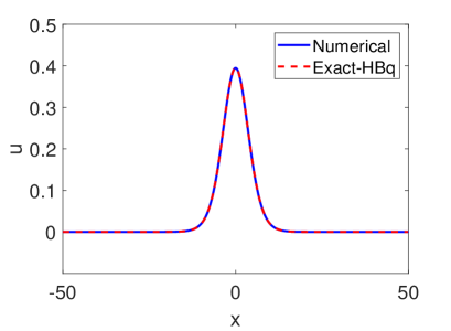
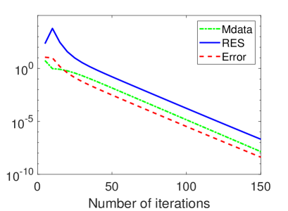
Figure 1: The solitary wave solution constructed by Petviashvili method for (1.1) and the exact solitary wave solution of the HBq equation for the speed $c=1.1272$ and the variation of the $Error(n)$, $|1-M_{n}|$ and $RES$ with the number of iterations in semi-log scale.

In order to test our scheme, we compare the solitary wave profile generated by the Petviashvili’s method for (1.1) ($\alpha=0,\kappa=1,p=1,\beta=1$) with the exact solitary wave solution of the HBq equation given in (5.19)-(5.21) ($\eta_{1}=\eta_{2}=1,p=2)$. The space interval is $-50\leq x\leq 50$ and we choose the the number of spatial grid points $N=1024$. Choosing $\eta_{1}=\eta_{2}=1,p=2$ in the equation (5.21), we compute the wave speed as $c=1.1272$. Then, taking the same wave speed, we generate the solitary wave profile by the Petviashvili’s method for (1.1) ($\alpha=0,\kappa=1,p=1,\beta=1$). In the left panel of Figure 1, we present the solitary wave solution constructed by Petviashvili method for (1.1) ($\alpha=0,\kappa=1,p=1,\beta=1$) with the exact solitary wave solution of the HBq equation. In the right panel of Figure 1, we show the variation of three different errors with the number of iterations in semi-log scale. As it seen from the figure, the solitary wave profile generated by Petviashvili’s method coincides with the exact solitary wave solution of the HBq equation which is a special case of the gBq equation. We also compute the $L_{\infty}$-error norm as $5.69\times 10^{-12}$.

5.1.2 Numerical generation of solitary waves for the gBq equation

To the best of authors’ knowledge, there is no exact solitary wave solution of the gBq equation where the parameter $\alpha$ is different from zero. It is natural to ask how the higher-order effects of dispersion and nonlinearity affect the solitary wave solutions. We now construct the solitary wave solution for some values of $\alpha,\kappa$ and $\beta$. The space interval is $-50\leq x\leq 50$ chosing the number of spatial grid points $N=1024$. We consider the quadratic nonlinearity $(p=1,f(u)=\beta u^{p+1})$.

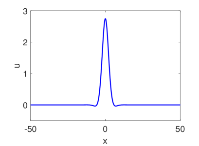
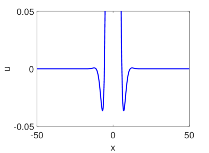
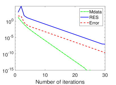
Figure 2: The solitary wave solution generated by the Petviashvili’s method for (1.1) with the parameters $\alpha=2$, $c=\sqrt{3},\kappa=\beta=1$ (top left), the close-up look at the profile (top right) and the variation of the $Error(n)$, $|1-M_{n}|$ and $RES$ with the number of iterations in semi-log scale (bottom).

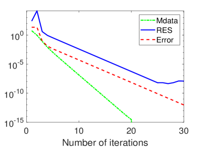
Figure 3: The solitary wave solution generated by the Petviashvili’s method for (1.1) with the parameters $\alpha=2$, $c=1.3,\kappa=\beta=1$ (left panel) and the variation of the $Error(n)$, $|1-M_{n}|$ and $RES$ with the number of iterations in semi-log scale (right panel).

The solitary wave profile generated by the Petviashvili’s method for the parameters $\alpha=2$, $c=\sqrt{3},\kappa=\beta=1$, where $c^{2}>\alpha>1$ is illustrated in the top left panel of Figure 2. The top right panel of Figure 2 gives a closer look. In the bottom panel, we present the variation of three different errors with the number of iterations in semi-log scale. The solitary wave profile generated by the Petviashvili’s method for the parameters $\alpha=2$, $c=1.3,\kappa=\beta=1$, where $1<c^{2}<\alpha$ is illustrated in the left panel of Figure 3. In the right panel of Figure 3, we present the variation of three different errors with the number of iterations in semi-log scale. As it seen from the Figures 2 and 3, the solitary wave solution has an oscillatory structure. For the parameters $(i)~{}\alpha=2,c=\sqrt{3},~{}\kappa=\beta=1$, $(ii)~{}\alpha=2,c=1.3,~{}\kappa=\beta=1$, the discriminant in (5.8) is calculated approximately as $-22.99,-4.56$, respectively. The presence of the imaginary parts of the roots, the solitary wave solution has oscillatory asymptotics. Therefore, the numerical results are compatible with the expected theoretical result.

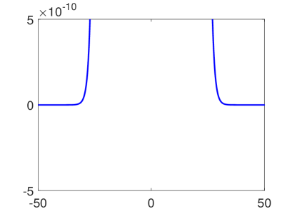
Figure 4: The solitary wave solution generated by the Petviashvili’s method for (1.1) with the parameters $\alpha=0.5,c=\sqrt{2.1},\kappa=0.1,\beta=1$ (left panel), the close-up look at the profile (right panel).

The solitary wave profile for the parameters $\alpha=0.5,c=\sqrt{2.1},\kappa=0.1,\beta=1$ is presented in the left panel of Figure 4. Contrary to the above experiments, we observe that (1.1) has the monotone sech-type solitary wave profile. The right panel of Figure 4 gives a closer look. It takes nonnegative values even if near zero. We observe that the equation (5.7) has four real roots for the chosen parameters. Therefore, the oscillatory asymptotic profile is disappered for this case.

6 Fourier pseudo-spectral numerical method for the gBq equation

In order to investigate the time evolution of the solutions for (1.1), we propose the numerical method combination of a Fourier pseudo-spectral method for the space component and a fourth-order Runge Kutta scheme (RK4) for time. If the spatial period $[-L,L]$ is, for convenience, normalized to $[0,2\pi]$ using the transformation $X=\pi(x+L)/L$, the equation (1.1) becomes

$$u_{tt} = \left(\frac{\pi}{L}\right)^{2}u_{XX}-\left(\frac{\pi}{L}\right)^{4}\alpha~{}u_{XXXX}+\left(\frac{\pi}{L}\right)^{2}u_{XXtt}-\left(\frac{\pi}{L}\right)^{4}\kappa~{}u_{XXXXtt}+(\frac{\pi}{L})^{2}\beta~{}(u^{p+1})_{XX}$$

The interval $[0,2\pi]$ is divided into $N$ equal subintervals with grid spacing $\Delta X=2\pi/N$, where the integer $N$ is even. The spatial grid points are given by $X_{j}=2\pi j/N$, $j=0,1,2,...,N$. The approximate solutions to $u(X_{j},t)$ is denoted by $U_{j}(t)$. The discrete Fourier transform of the sequence $\{U_{j}\}$

$$\widetilde{U}_{k}={\cal F}_{k}[U_{j}]=\frac{1}{N}\sum_{j=0}^{N-1}U_{j}\exp(-ikX_{j}),~{}~{}~{}~{}-\frac{N}{2}\leq k\leq\frac{N}{2}-1~{}$$ (6.2)

gives the corresponding Fourier coefficients. Similarly, $\{U_{j}\}$ can be recovered from the Fourier coefficients by the inversion formula for the discrete Fourier transform (6.2)

$$U_{j}={\cal F}^{-1}_{j}[\widetilde{U}_{k}]=\sum_{k=-\frac{N}{2}}^{\frac{N}{2}-1}\widetilde{U}_{k}\exp(ikX_{j}),~{}~{}~{}~{}j=0,1,2,...,N-1.$$ (6.3)

Here $\cal F$ denotes the discrete Fourier transform and ${\cal F}^{-1}$ its inverse. These transforms are performed using the well-known software package FFT algorithm in Matlab.

Applying the discrete Fourier transform to the equation (6), the system of ordinary differential equations is given explicitly

$$(\widetilde{U}_{k})_{t}=\widetilde{V}_{k}$$ (6.4)

$$(\widetilde{V}_{k})_{t}=-\frac{\Big{\{}\big{[}(\pi k/L)^{2}+\alpha(\pi k/L)^{4}\big{]}\widetilde{U}_{k}+\beta(\pi k/L)^{2}(\widetilde{U^{p+1}})_{k}\Big{\}}}{1+(\pi k/L)^{2}+\kappa(\pi k/L)^{4}}$$ (6.5)

We use the fourth-order Runge-Kutta method to solve the system of ordinary differential equations (6.4)-(6.5) in time. Finally, we find the approximate solution by using the inverse Fourier transform (6.3).

6.1 Time evolution of the single solitary wave

The aim of this subsection is to investigate the time evolution of the single solitary wave solution of (1.1). First we show that our proposed method is capable of high accuracy and to confirm the convergence of the scheme in space and time. The $L_{\infty}$-error norm is defined as

$$L_{\infty}\mbox{-error}=\max_{i}|~{}u_{i}-U_{i}~{}|,$$ (6.6)

where $u_{i}$ denotes the exact solution at $u(X_{i},t)$.

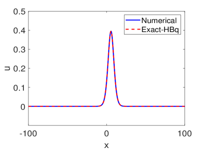
Figure 5: The solitary wave solution obtained by the Fourier pseudo-spectral scheme for (1.1) with $\alpha=0$ and the exact solitary wave solution for the HBq equation

In the first numerical experiment, we take the initial data

$$u(x,0)=\frac{15}{38}\,\operatorname{sech}^{4}(\frac{x}{2\sqrt{13}})$$ (6.7)

$$v(x,0)=\frac{15\sqrt{13}}{19\sqrt{133}}\operatorname{sech}^{4}(\frac{x}{2\sqrt{13}})\tanh(\frac{x}{2\sqrt{13}})$$ (6.8)

corresponding to the solitary wave solution (5.19) for $\eta_{1}=\eta_{2}=1,p=2$ initially located at $x_{0}=0$. The experiment was run from $t=0$ to $t=5$ in the space interval $-100\leq x\leq 100$ taking the number of spatial grid points $N=2048$ and the number of temporal grid points $M=1000$. To test the accuracy of the scheme (6.4)-(6.5), the numerical solution obtained for (1.1) with $\alpha=0$ is compared with the exact solitary wave solution for the HBq equation (5.19) at $t=5$ in Figure 5. As it is seen from the Figure 5, the numerical solution and the exact solution coincide very well. The $L_{\infty}$-error norm at $t=5$ is $8.33\times 10^{-16}$. It shows that our proposed method is capable of high accuracy.

Figure 6: The convergence rates in time calculated from the $L_{\infty}$-errors (left panel) and in space calculated from the $L_{\infty}$-errors (right panel).

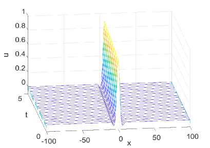
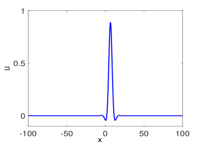
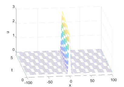
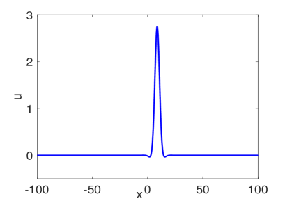
Figure 7: Evolution of the solitary wave (top left), the profile at $t=5$ (top right) for the parameters $\alpha=2,c=1.3$, $\kappa=\beta=1$ and the evolution of the solitary wave (bottom left), the profile at $t=5$ (bottom right) for the parameters $\alpha=2,c=\sqrt{3},\kappa=\beta=1$.

Our goal is to understand numerically how the higher-order effects of dispersion and nonlinearity affect the solitary wave solutions of (1.1) as time increases. Therefore, we need an initial conditions for $u(x,0)$ and $u_{t}(x,0)$. The generated solitary wave profile $Q_{c}$ using Petviashvili’s iteration method for the parameters $\alpha=2,c=1.3,\kappa=\beta=1$ is taken as $u(x,0)$. Since the localized solitary wave solution has the form $u(x,t)=Q_{c}(x-ct)$, we get $u_{t}(x,t)=-cQ_{c}^{\prime}(x-ct)$. We set $u_{t}(x,0)=-cQ_{c}^{\prime}(x)$. It is computed by $-c{\cal F}_{j}^{-1}[ik{\cal F}_{k}[Q_{c}(j)]]$ numerically. Since the exact solitary wave solution is unknown, the “exact” solitary wave solution $u^{\rm ex}$ is obtained numerically with a very fine spatial step size $N=1024$ and a very small time step $M=5000$ by using Fourier pseudo-spectral method.

In order to test the temporal discretization errors for the gBq equation where the parameter $\alpha$ is different from zero, we fix the number of spatial grid points $N=1024$ and solve (1.1) for different time step $\tau$. The convergence rates calculated from the $L_{\infty}$-errors at the terminating time $t=5$ are illustrated in the left panel of Figure 6. The computed convergence rates agree well with the fact that Fourier pseudo-spectral method exhibits the fourth-order convergence in time. In order to test the spatial discretization errors, we fix the the time step $(\tau=0.001)$ such that the temporal error can be neglected, and solve (1.1) for different spatial step size $h$. The right panel of Figure 6 shows the variation of $L_{\infty}$-errors with spatial step size. The error decays very rapidly when the spatial step size decreases. These results show that the numerical solution obtained using the Fourier pseudo-spectral scheme converges rapidly to the accurate solution in space.

Figure 7 shows evolution of the oscillatory solitary wave for the parameters $(i)~{}\alpha=2,c=\sqrt{3}$ , $\kappa=1$ (top left panel), $(ii)~{}\alpha=2,c=1.3,\kappa=1$ (bottom left panel). We also present the solitary wave profile at the final time $t=5$. The experiment was run from $t=0$ to $t=5$ in the space interval $-100\leq x\leq 100$ taking the number of spatial grid points $N=1024$ and the number of temporal grid points $M=5000$. As it seen from the figure, the solitary wave emerges without any change in their shapes. We do not observe any dispersive tail as time increases.

6.2 Global and Blow-up Solutions

In this subsection, we first test the ability of the proposed method investigating the global existence and blow-up solutions of the gBq equation. The analytical results needed for the global existence or blow-up of the solutions for (1.1) have been discussed in Section 2 but there remains a gap between the global existence and blow-up intervals. Our aim is to give a shed of light for the gap interval neither a global existence nor a blow-up result is established.

For the numerical experiments in this subsection, the problem is solved on the interval $-100\leq x\leq 100$ taking the spatial grid points as $N=2048$. In the rest of the study, we consider (1.1) with cubic nonlinearity $f(u)=-u^{3}$ setting the parameters $\alpha=\kappa=1$ and $\beta=-1$ in (1.1). The steady state solution of the equation

$$u-u^{\prime\prime}-u^{3}=0$$

is given by $g(x)=\sqrt{2}\operatorname{sech}(x)$. If we choose the initial data

$$u(x,0)=-\sqrt{2}A\operatorname{sech}(x)\tanh(x),\hskip 30.0ptv(x,0)=0,$$ (6.9)

where $A>0$, one gets

$$d = J(g)=\frac{1}{2}\|g\|_{H^{1}}^{2}-\frac{1}{4}\|g\|_{L^{4}}^{4}=\frac{4}{3},$$

$$E(u(x,0)) = \frac{1}{2}\left(\|u(\cdot,0)\|_{L^{2}}^{2}+\|v(\cdot,0)\|_{L^{2}}^{2}+\|u_{x}(\cdot,0)\|_{L^{2}}^{2}+\|v_{x}(\cdot,0)\|_{L^{2}}^{2}+\|(-\partial_{x}^{2})^{-1/2}v(.,0)\|_{L^{2}}^{2}\right)$$

$$\hskip 15.0pt-\frac{1}{4}\|u(\cdot,0)\|_{L^{4}}^{4}$$

$$= \frac{4A^{2}}{35}(14-A^{2}),$$

$$I(u(x,0)) = \|u(.,0)\|_{H^{1}}^{2}-\|u(\cdot,0)\|_{L^{4}}^{4}=\frac{16A^{2}}{35}(7-A^{2}).$$

Thus we obtain that

$$E(u(x,0)) < d\Leftrightarrow A\in(0,0.943)\cup(3.621,\infty)$$

$$I(u(x,0) < 0\Leftrightarrow A>\sqrt{7}\approx 2.646.$$

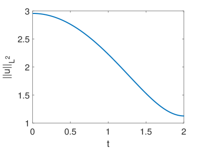
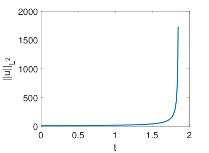
Figure 8: The variation of the $L^{2}$-norm of the approximate solution for $A=0.8$ (left panel) and $A=3.7$ (right panel).

We present the variation of the $L^{2}$-norm of the approximate solution obtained using the Fourier pseudo-spectral scheme for $A=0.8$ and $A=3.7$ in Figure 8. In the left panel of Figure 8, the $L^{2}$-norm of the approximate solution solution decreases as time increases for $A=0.8$. The numerical result indicates the global existence of the solution. This numerical result is also compatible with the analytical result given in Theorem $2.6$. In the right panel of Figure 8, the $L^{2}$-norm of the approximate solution solution increases as time increases for $A=3.7$. This is a strong indication of that the solutions blow-up in finite time. This numerical result is in complete agreement with the analytical result given in Theorem $2.7$.

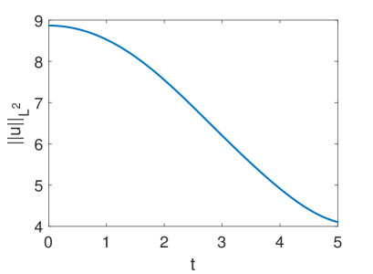
Figure 9: The variation of the $L^{2}$-norm of the approximate solution for $A=2.4$ (left panel) and $A=2.5$ (right panel).

There is no analytical result for the gap interval $A\in[0.943,3.621]$. We performed lots of numerical experiments for different parameters of $A$. The numerical experiments indicate that there is a thereshold value $A^{*}\in(2.4,2.5)$ such that the solution exists globally for $A\in[0.943,A^{*})$ and it blows-up in finite time for $A\in[A^{*},3.621]$. The variation of the $L^{2}$-norm of the approximate solution is illustrated for $A=2.4$ and $A=2.5$ in Figure 9. The $L^{2}$-norm of the approximate solution decreases as time increases for $A=2.4$ which indicates the global existence of the solution. If $A=2.5$, then the $L^{2}$-norm of the approximate solution increases as time increases for $A=2.5$ which shows the solution blows-up in finite time.

In the second numerical experiment, we take the initial data

$$u(x,0)=v(x,0)=-\sqrt{2}A\operatorname{sech}(x)\tanh(x)$$ (6.10)

where $A>0$. It yields

$$E(u(x,0))=A^{2}\left(\frac{78}{15}-\frac{4}{35}A^{2}\right),$$

and

$$E(u(x,0)) < d\Leftrightarrow A\in(0,0.508)\cup(6.726,\infty),$$

$$I(u(x,0) < 0\Leftrightarrow A>\sqrt{7}\approx 2.646.$$

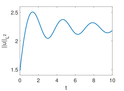
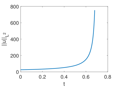
Figure 10: The variation of the $L^{2}$-norm of the approximate solution for $A=0.4$ (left panel) and $A=7$ (right panel).

In the left panel of Figure 10, the $L^{2}$-norm of the approximate solution solution remains bounded for $A=0.4$. It oscillates as time increases. The numerical result indicates the global existence of the solution. This numerical result is also compatible with the analytical result given in Theorem $2.6$ since $E(u(x,0)<d$ and $I(u(x,0))>0$. The $L^{2}$-norm of the approximate solution solution increases as time increases for $A=7$. This is a strong indication of that the solutions blow-up in finite time. This numerical result is in complete agreement with the analytical result given in Theorem $2.7$.

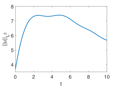
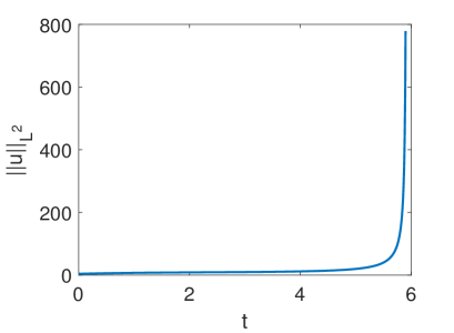
Figure 11: The variation of the $L^{2}$-norm of the approximate solution for $A=1$ (left panel) and $A=1.1$ (right panel).

For the gap interval $A\in[0.508,6.726]$, the numerical experiments indicate that there is a thereshold value $A^{*}\in(1,1.1)$ such that the solution exists globally for the parameter $A\in[0.508,A^{*})$ and it blows-up in finite time for time parameter $A\in[A^{*},6.726]$. The variation of the $L^{2}$-norm of the approximate solutions are illustrated for $A=1$ and $A=1.1$ in Figure 11.

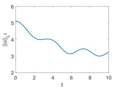
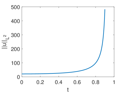
Figure 12: The variation of the $L^{2}$-norm of the approximate solution for $A=1.6$ (left panel) and $A=6.5$ (right panel).

In the last numerical experiment, we take the initial data

$$u(x,0)=A\Big{[}g(x)-\frac{1}{2}g(x-1)-\frac{1}{2}g(x+1)\Big{]},\hskip 30.0ptv(x,0)=0,$$ (6.11)

where $A>0$. It yields

$$E(u(x,0)) < d\Leftrightarrow A\in(0,1.728)\cup(6.435,\infty),$$

$$I(u(x,0) < 0\Leftrightarrow A>4.712.$$

The $L^{2}$-norm of the approximate solutions correspond to $A=1.6$ and $A=6.5$ are depicted in Figure 12. The $L^{2}$-norm of the approximate solution solution decreases with oscillations $A=1.6$. It remains bounded. The numerical result indicates the global existence of the solution which is compatible with the Theorem $2.6$. The $L^{2}$-norm of the approximate solution solution increases as time increases for $A=6.5$. This is a strong indication of that the solutions blow-up in finite time which is compatible with Theorem $2.7$.

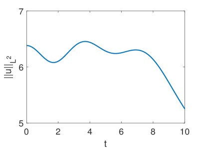
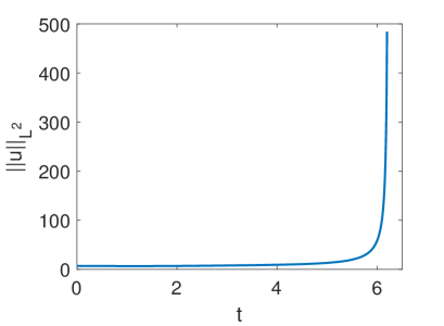
Figure 13: The variation of the $L^{2}$-norm of the approximate solution for $A=2$ (left panel) and $A=2.1$ (right panel).

For the gap interval $A\in[1.728,6.435]$, the numerical experiments indicate that there is a thereshold value $A^{*}\in(2,2.1)$ such that the solution exists globally for the parameter $A\in[1.728,A^{*})$ and it blows-up in finite time for time parameter $A\in[A^{*},6.435]$. The variation of the $L^{2}$-norm of the approximate solution is illustrated for $A=2$ and $A=2.1$ in Figure 13.

References

- [1] H. Borluk, G. M. Muslu, A Fourier pseudospectral method for a generalized improved Boussinesq equation, Numer. Methods Partial Differ. Equ. 31 (2015) 995–1008.
- [2] J.V. Boussinesq, Théorie des ondes et des remous qui se propagent le long dun canal rectangulaire horizontal, en communiquant au liquide contene dans ce canal des vitesses sensiblement pareilles de la surface au fond, J. Math. Pures Appl. 17 (1872) 55–108.
- [3] A. G. Bratsos, A predictor-corrector scheme for the improved Boussinesq equation, Chaos Soliton Fract. 40 (2009) 2083–2094.
- [4] C.I. Christov, G.A. Maugin, M.G. Velarde, Well-posed Boussinesq paradigm with purely spatial higherorder derivatives, Phy. Rev. E 54 (1996) 3621–3638.
- [5] A. Córdoba, Á.D. Martínez, A pointwise inequality for fractional Laplacians, Adv. Math. 280 (2015) 79–85.
- [6] Q. Deng, Y. Ding, X. Yao, Gaussian bounds for higher-order elliptic differential operators with Kato type potentials, J. Funct. Anal. 266 (2014) 5377–5397.
- [7] N. Duruk, A. Erkip, H. A. Erbay, A higher-order Boussinesq equation in locally non-linear theory of one-dimensional non-local elasticity, IMA J. Appl. Math. 74 (2009) 97-106.
- [8] A. Esfahani, L.G. Farah, H. Wang, Global existence and blow-up for the generalized sixth-order Boussinesq equation, Nonlinear Anal. 75 (2012) 4325–4338.
- [9] A. Esfahani, S. Levandosky, Stability of solitary waves for the generalized higher-order Boussinesq equation, J. Dynam. Diff. Equations 24 (2012) 391–425.
- [10] J. D. Frutos, T. Ortega and J. M. Sanz-Serna, Pseudospectral method for the good Boussinesq equation, Math. Comput. 57 (1991) 109–122.
- [11] G.H. Keulegan, G.W. Patterson, Mathematical theory of irrotational translation waves, J. Res. Natl. Bur. Stand. 24 (1940) 47–101.
- [12] C.E. Kenig, G. Ponce, L. Vega, Well-posedness and scattering results for the generalized Korteweg-de Vries equation via the contraction principle, Commun. Pure App. Math. 46 (1993) 527–620.
- [13] H.A. Levine, Some additional remarks on the nonexistence of global solutions to nonlinear equations, SIAM J. Math. Anal. 5 (1974) 138–146.
- [14] F. Linares, Global existence of small solutions for a generalized Boussinesq equation, J. Diff. Equations 106 (1993) 257–293.
- [15] F. Linares, G. Ponce, Gustavo, Introduction to nonlinear dispersive equations, Second edition, Universitext, Springer, New York, 2015.
- [16] Y. Liu, Decay and scattering of small solutions of a generalized Boussinesq equation, J. Funct. Anal. 147 (1997) 51–68.
- [17] R.L. Pego, M.I. Weinstein, On the strong spectral stability of some Boussinesq solitary waves, Structure and Dynamics of Nonlinear Waves in Fluids, A. Mielke, K. Kirchgässner, eds., World Scientific, Singapore, 1995, pp. 370–382.
- [18] D. Pelinovsky, Y. Stepanyants, Convergence of Petviashvili’s iteration method for numerical approximation of stationary solution of nonlinear wave equations, SIAM J. Numer. Anal. 42 (2004) 1110–1127.
- [19] V.I. Petviahvili, Equation of an extraordinary soliton, Plasma Physics 2 (1976) 469–472.
- [20] P. Rosenau, Dynamics of dense discrete systems: High order effects, Prog. Theor. Phys. 79 (1988) 1028–1042.
- [21] X. Runzhang, L. Yacheng, L. Bowei, The Cauchy problem for a class of the multidimensional Boussinesq-type equation, Nonlinear Analysis 74 (2011) 2425–2437.
- [22] G. Schneider, The long wave limit for a Boussinesq equation, SIAM J. Appl. Math. 58 (1998) 1237–1245.
- [23] G. Schneider, C.W. Eugene, Kawahara dynamics in dispersive media, Physica D 152-153 (2001) 384–394.
- [24] A. Shokri, M. Dehghan, A not-a-knot meshless method using radial basis functions and predictor-corrector scheme to the numerical solution of improved Boussinesq equation, Comput. Phys. Commun. 181 (2010) 1990–2000.
- [25] E.M. Stein, Oscillatory integrals in Fourier analysis, in : Beijing Lectures in Harmonic Analysis, Princeton Press, 1986, pp. 307–355.
- [26] C. Su, G.M. Muslu, An exponential integrator sine pseudospectral method for the generalized improved Boussinesq equation, BIT Numer. Math. 61 (2021) 1397–1419.
- [27] G. Topkarci, H. Borluk, G.M. Muslu, Higher order dispersive effects in regularized Boussinesq equation, Wave Motion 68 (2017) 272–282.
- [28] M. Tsutsimi, T. Matahashi, On the Cauchy problem for the Boussinesq type equation, Math. Jap. 36 (1991) 371–379.
- [29] S. Wang, G. Xu, The Cauchy problem for the Rosenau equation, Nonlinear Anal. 71 (2009) 456–466.
- [30] J. Yang, Nonlinear waves in integrable and nonintegrable systems, SIAM, 2010.