[a]Andrei Rabusov

Partial wave analysis of $\mathup{{{\uptau}}^{\scriptstyle{-}}}\mspace{1.0mu}\to\mspace{1.0mu}\mathup{{{\uppi}}^{\scriptstyle{-}}}\mathup{{{\uppi}}^{\scriptstyle{+}}}\mathup{{{\uppi}}^{\scriptstyle{-}}}\mathup{{{\upnu}}{}_{\scriptstyle{\!\uptau}}}$ at Belle

Abstract

We present simulation studies in preparation for analyzing $\mathup{{{\uptau}}^{\scriptstyle{-}}}\mspace{1.0mu}\to\mspace{1.0mu}\mathup{{{\uppi}}^{\scriptstyle{-}}}\mathup{{{\uppi}}^{\scriptstyle{+}}}\mathup{{{\uppi}}^{\scriptstyle{-}}}\mathup{{{\upnu}}{}_{\scriptstyle{\!\uptau}}}$ in data from the Belle experiment at the KEK $\mathup{{{e}}^{\scriptstyle{+}}}\mathup{{{e}}^{\scriptstyle{-}}}$ collider. Analyzing this decay can shed light on the ${\mathup{{{a}}{}_{\scriptstyle{1}}}}{\mathup{{\left({1260}\right)}}}$ and ${\mathup{{{a}}{}_{\scriptstyle{1}}}}{\mathup{{\left({1420}\right)}}}$ resonances and yield results that improve measurement of the $\mathup{{{\uptau}}}$ electric and magnetic dipole moments. We show that we can achieve a higher signal efficiency than previous analyses of the same decay. We also demonstrate that neural networks can model our complicated six-dimensional background distributions and that quasi-model-independent partial-wave analysis can extract resonance masses, widths, and production amplitudes and phases.

In the decay $\mathup{{{\uptau}}^{\scriptstyle{-}}}\mspace{1.0mu}\to\mspace{1.0mu}\mathup{{{\uppi}}^{\scriptstyle{-}}}\mathup{{{\uppi}}^{\scriptstyle{+}}}\mathup{{{\uppi}}^{\scriptstyle{-}}}\mathup{{{\upnu}}{}_{\scriptstyle{\!\uptau}}}$, hadrons are produced from unflavored axial-vector resonances [1]. This is an opportune setting in which to study such composite particles without strong interaction with other particles that may alter their resonance shapes. The dominantly produced resonance is the ${\mathup{{{a}}{}_{\scriptstyle{1}}}}{\mathup{{\left({1260}\right)}}}$, whose shape is much debated and whose mass and width are not well determined [2, 3, 4]. The COMPASS experiment observed an unexpected narrow axial-vector resonance, ${\mathup{{{a}}{}_{\scriptstyle{1}}}}{\mathup{{\left({1420}\right)}}}$, in partial-wave analysis (PWA) of three-pion final states produced in pion-proton scattering [5]. Whether this is a true particle resonance or an effect of $\mathup{{{K}}^{\scriptstyle{\ast}}}\mathup{{{K}}}$ scattering is debated [6].

A better model for $\mathup{{{\uptau}}^{\scriptstyle{-}}}\mspace{1.0mu}\to\mspace{1.0mu}\mathup{{{\uppi}}^{\scriptstyle{-}}}\mathup{{{\uppi}}^{\scriptstyle{+}}}\mathup{{{\uppi}}^{\scriptstyle{-}}}\mathup{{{\upnu}}{}_{\scriptstyle{\!\uptau}}}$, driven by experimental measurement, will improve the simulation of this decay in existing MC generators, which is necessary for general $\mathup{{{\uptau}}}$ studies at currently running experiments such as Belle II [7]. In particular, it will improve measurement of the tauon electric and magnetic dipole moments [8].

The Belle experiment, which ran for a decade at the $10.58$-$\mathrm{G}\mathrm{e}\mathrm{V}$ $\mathup{{{e}}^{\scriptstyle{+}}}\mathup{{{e}}^{\scriptstyle{-}}}$ collider KEKB in Tsukuba, Japan, can study the ${\mathup{{{a}}{}_{\scriptstyle{1}}}}{\mathup{{\left({1260}\right)}}}$ and ${\mathup{{{a}}{}_{\scriptstyle{1}}}}{\mathup{{\left({1420}\right)}}}$ and the general structure of $\mathup{{{\uptau}}^{\scriptstyle{-}}}\mspace{1.0mu}\to\mspace{1.0mu}\mathup{{{\uppi}}^{\scriptstyle{-}}}\mathup{{{\uppi}}^{\scriptstyle{+}}}\mathup{{{\uppi}}^{\scriptstyle{-}}}\mathup{{{\upnu}}{}_{\scriptstyle{\!\uptau}}}$ using partial-wave analysis and data containing $50\text{\times}{10}^{6}$ $\mathup{{{\uptau}}^{\scriptstyle{-}}}\mspace{1.0mu}\to\mspace{1.0mu}\mathup{{{\uppi}}^{\scriptstyle{-}}}\mathup{{{\uppi}}^{\scriptstyle{+}}}\mathup{{{\uppi}}^{\scriptstyle{-}}}\mathup{{{\upnu}}{}_{\scriptstyle{\!\uptau}}}$ decays [9]. This data size is comparable to that of the COMPASS experiment, five and fifty times larger than what the Belle and Babar experiments used to publish $\mathup{{{\uppi}}}\mathup{{{\uppi}}}\mathup{{{\uppi}}}$ mass spectra, and one-thousand times larger than what the CLEO II experiment used to publish the only amplitude analysis of $\mathup{{{\uptau}}^{\scriptstyle{-}}}\mspace{1.0mu}\to\mspace{1.0mu}\mathup{{{\uppi}}}\mathup{{{\uppi}}}\mathup{{{\uppi}}}\mathup{{{\upnu}}{}_{\scriptstyle{\!\uptau}}}$ [5, 10, 11, 3].

We present preliminary studies of the applicability of PWA to $\mathup{{{\uptau}}^{\scriptstyle{-}}}\mspace{1.0mu}\to\mspace{1.0mu}\mathup{{{\uppi}}^{\scriptstyle{-}}}\mathup{{{\uppi}}^{\scriptstyle{+}}}\mathup{{{\uppi}}^{\scriptstyle{-}}}\mathup{{{\upnu}}{}_{\scriptstyle{\!\uptau}}}$ using simulated data. Since Belle cannot detect neutrinos and $\mathup{{{\uptau}}}$ decays are measured in events with at least two neutrinos, we do not know the full coordinate of each decay in its eight-dimensional phase space. We analyze in a six-dimensional subspace spanned by the three-pion mass, $m_{3\mathup{{{\uppi}}}}$, the two $\mathup{{{\uppi}}^{\scriptstyle{+}}}\mathup{{{\uppi}}^{\scriptstyle{-}}}$ squared masses, $s_{1}$ and $s_{2}$, and the three Euler angles, $\alpha$, $\beta$, and $\gamma$, defined in [12]. We average decay rates over the unknown neutrino direction and calculate them from hadronic currents written in the relativistic tensor formalism of [13].

We study data simulated as if it is produced by the Belle experiment, with all known interactions originating from $\mathup{{{e}}^{\scriptstyle{+}}}\mathup{{{e}}^{\scriptstyle{-}}}$ collision, including $\mathup{{{e}}^{\scriptstyle{+}}}\mathup{{{e}}^{\scriptstyle{-}}}\to\mathup{{{\uptau}}^{\scriptstyle{+}}}\mathup{{{\uptau}}^{\scriptstyle{-}}}$. To isolate $\mathup{{{\uptau}}^{\scriptstyle{+}}}\mathup{{{\uptau}}^{\scriptstyle{-}}}$ events containing $\mathup{{{\uptau}}^{\scriptstyle{-}}}\mspace{1.0mu}\to\mspace{1.0mu}\mathup{{{\uppi}}^{\scriptstyle{-}}}\mathup{{{\uppi}}^{\scriptstyle{+}}}\mathup{{{\uppi}}^{\scriptstyle{-}}}\mathup{{{\upnu}}{}_{\scriptstyle{\!\uptau}}}$, we select events that each have four charged particles, having total charge zero, coming from the $\mathup{{{e}}^{\scriptstyle{+}}}\mathup{{{e}}^{\scriptstyle{-}}}$ interaction region, each with transverse momentum in the lab frame above $100\text{\,}\mathrm{M}\mathrm{e}\mathrm{V}$. We select events with a $3{\times}1$ topology relative to the thrust axis in the $\mathup{{{e}}^{\scriptstyle{+}}}\mathup{{{e}}^{\scriptstyle{-}}}$ center-of-momentum (CM) frame.

We use a boosted-decision-tree algorithm (BDT) from the ROOT TMVA library to further select signal decays and veto background events; it looks at six event-wide kinematic variables. After selecting events by their BDT score, we further select for pion-identification quality and veto events in which any pair of oppositely charged pions are consistent with coming from a $\mathup{{{K}}{}_{\scriptstyle{S}}^{\scriptstyle{0}}}$ or in which the total energy of photons in the signal hemisphere is consistent with the presence of one or more $\mathup{{{\uppi}}^{\scriptstyle{0}}}$. Photons counted for the veto must have energy above $40\text{\,}\mathrm{M}\mathrm{e}\mathrm{V}$ in the lab frame. Our signal efficiency is $31$%, with a signal purity of $87$%.

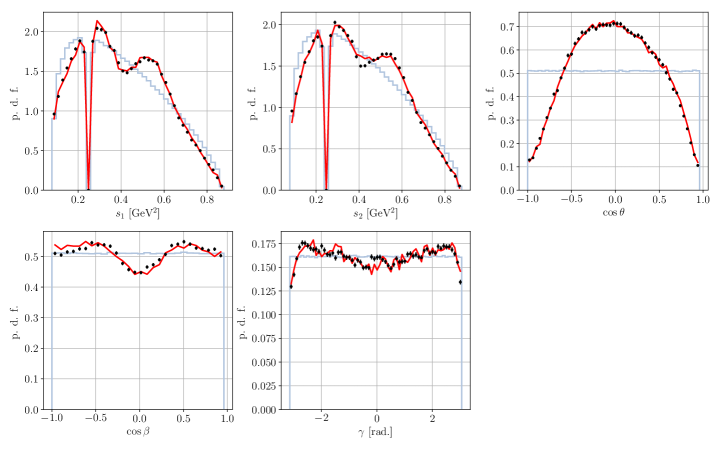
Figure 1: Distribution in simulation (black), from neural-network (red), and structureless (blue)

The other $13$% of events are from $\mathup{{{e}}^{\scriptstyle{+}}}\mathup{{{e}}^{\scriptstyle{-}}}\mspace{1.0mu}\to\mspace{1.0mu}\mathup{{{\uptau}}^{\scriptstyle{+}}}\mathup{{{\uptau}}^{\scriptstyle{-}}}$ in which the three-prong tau decay is $\mathup{{{\uptau}}^{\scriptstyle{-}}}\mspace{1.0mu}\to\mspace{1.0mu}\mathup{{{\uppi}}^{\scriptstyle{-}}}\mathup{{{\uppi}}^{\scriptstyle{+}}}\mathup{{{\uppi}}^{\scriptstyle{-}}}\mathup{{{\uppi}}^{\scriptstyle{0}}}\mathup{{{\upnu}}{}_{\scriptstyle{\!\uptau}}}$ (with possible further $\mathup{{{\uppi}}^{\scriptstyle{0}}}$) or $\mathup{{{\uptau}}^{\scriptstyle{-}}}\mspace{1.0mu}\to\mspace{1.0mu}\mathup{{{K}}^{\scriptstyle{-}}}\mathup{{{\uppi}}^{\scriptstyle{+}}}\mathup{{{\uppi}}^{\scriptstyle{-}}}\mathup{{{\upnu}}{}_{\scriptstyle{\!\uptau}}}$ or from $\mathup{{{e}}^{\scriptstyle{+}}}\mathup{{{e}}^{\scriptstyle{-}}}\mspace{1.0mu}\to\mspace{1.0mu}\mathit{{q}{}_{\mspace{-3.0mu}\scriptstyle{}}^{\mspace{-1.0mu}\scriptstyle{}}}\mathit{{\mkern 4.0mu\overline{\mkern-4.0mu{q}}}{}_{\mspace{-2.0mu}\scriptstyle{}}^{\mspace{0.0mu}\scriptstyle{}}}$. The dynamic structure of these backgrounds in the 6D analysis space is too complicated to model parametrically. Instead we let a neural network learn the background shape, a method pioneered in amplitude analysis by LHCb in [14] to use a single neural network to parametrize the background in the entire phase space. We find it necessary to train multiple neural networks, each for a subregion of $m(3\uppi)$. Fig. 1 shows the resulting background shape for $m_{3\mathup{{{\uppi}}}}\in$1.061.08\text{\,}\mathrm{G}\mathrm{e}\mathrm{V}$$. The neural network prediction agrees with the simulated background.

We analyze the data in subregions of $m_{3\uppi}$ with background modeled by the neural network and signal modeled with isobars and quasi-model-independent partial-wave analysis (QMIPWA) as described in [15]. To cross check the method, we analyze data simulated with only four partial waves: $1^{+}[{\mathup{{{f}}{}_{\scriptstyle{0}}}}{\mathup{{\left({980}\right)}}}\mathup{{{\uppi}}}]_{\text{P}}$, $1^{+}[\uprho(770)\mathup{{{\uppi}}}]_{\text{S}}$, $1^{+}[\uprho(770)\mathup{{{\uppi}}}]_{\text{D}}$, and $1^{+}[{\mathup{{{f}}{}_{\scriptstyle{2}}}}{\mathup{{\left({1270}\right)}}}\mathup{{{\uppi}}}]_{\text{P}}$. We use a QMIPWA isobar for the $1^{+}[1^{--}\mathup{{{\uppi}}}]_{\text{S}}$ wave only, to avoid zero modes and simplify the test. We fit the QMIPWA complex amplitudes and a complex multiplier for each remaning wave. We then fit a Breit-Wigner function to the QMIPWA results (Fig. 2). The second fit determines the $\uprho$’s mass and width to be $769.8\pm 0.6\text{\,}\mathrm{M}\mathrm{e}\mathrm{V}$ and $155.2\pm 1.3\text{\,}\mathrm{M}\mathrm{e}\mathrm{V}$, agreeing with the simulated values of $769.0\text{\,}\mathrm{M}\mathrm{e}\mathrm{V}$ and $150.9\text{\,}\mathrm{M}\mathrm{e}\mathrm{V}$. The fit results (Table 1) all agree with their simulated values.

Wave	Amplitude			Phase [deg]
	sim.	res.		sim.	res.
$[{\mathup{{{f}}{}_{\scriptstyle{0}}}}{\mathup{{\left({980}\right)}}}\mathup{{{\uppi}}}]_{\text{P}}$	$0.10$	$0.099$$\,\pm\,$	$0.001$	$-60$	$-55.485$$\,\pm\,$	$1.947$
$[\uprho(770)\mathup{{{\uppi}}}]_{\text{S}}$	$0.70$	$0.712$$\,\pm\,$	$0.005$	$0$	reference phase
$[\uprho(770)\mathup{{{\uppi}}}]_{\text{D}}$	$0.92$	$0.959$$\,\pm\,$	$0.025$	$120$	$120.546$$\,\pm\,$	$0.459$
$[{\mathup{{{f}}{}_{\scriptstyle{2}}}}{\mathup{{\left({1270}\right)}}}\mathup{{{\uppi}}}]_{\text{P}}$	$0.53$	$0.514$$\,\pm\,$	$0.020$	$15$	$18.255$$\,\pm\,$	$2.525$

Table 1: Comparison of simulated values and fit results. Figure 2: QMIPWA (violet) and Breit-Wigner (orange) fit results for the $1^{+}[1^{--}\mathup{{{\uppi}}}]_{\text{S}}$ wave in simulated data; elipses show 68%-confidence intervals.

In conclusion, we have developed selection criteria with higher efficiency than previously achieved by the BaBar and Belle experiments [11, 10], though with a higher background contamination. However, we can still analyze this data well using a neural-network to parameterize background. We have also demonstrated that a fit algorithm using quasi-model-independent partial-wave analysis reproduces simulation inputs. This technique will be useful to study the ${\mathup{{{a}}{}_{\scriptstyle{1}}}}{\mathup{{\left({1260}\right)}}}$, ${\mathup{{{a}}{}_{\scriptstyle{1}}}}{\mathup{{\left({1420}\right)}}}$, ${\mathup{{{a}}{}_{\scriptstyle{1}}}}{\mathup{{\left({1640}\right)}}}$ and general structure of $\mathup{{{\uptau}}^{\scriptstyle{-}}}\mspace{1.0mu}\to\mspace{1.0mu}\mathup{{{\uppi}}^{\scriptstyle{-}}}\mathup{{{\uppi}}^{\scriptstyle{+}}}\mathup{{{\uppi}}^{\scriptstyle{-}}}\mathup{{{\upnu}}{}_{\scriptstyle{\!\uptau}}}$ independent of a model.

References

• [1] G. Alexander et al., Evidence for the $\uptau\to\upnu\uprho\uppi$ decay mode, Physics Letters B 73 (1978) 99.
• [2] M. Aghasyan et al., Light isovector resonances in ${\uppi}^{-}p\rightarrow{\uppi}^{-}{\uppi}^{-}{\uppi}^{+}p$ at $190\text{ }\text{ }\mathrm{GeV}/c$, Phys. Rev. D 98 (2018) 092003.
• [3] CLEO Collaboration collaboration, Hadronic structure in the decay ${\uptau}^{-}\rightarrow{\upnu}_{\uptau}{\uppi}^{-}{\uppi}^{0}{\uppi}^{0}$ and the sign of the tau neutrino helicity, Phys. Rev. D 61 (1999) 012002.
• [4] P.D. Group, P.A. Zyla, R.M. Barnett, J. Beringer, O. Dahl, D.A. Dwyer et al., Review of Particle Physics, Progress of Theoretical and Experimental Physics 2020 (2020) .
• [5] COMPASS Collaboration collaboration, Observation of a new narrow axial-vector meson ${a}_{1}(1420)$, Phys. Rev. Lett. 115 (2015) 082001.
• [6] M. Mikhasenko, B. Ketzer and A. Sarantsev, Nature of the ${a}_{1}(1420)$, Phys. Rev. D 91 (2015) .
• [7] E. Kou et al., The Belle II Physics Book, Progress of Theoretical and Experimental Physics 2019 (2019) .
• [8] F. Krinner and S. Paul, Precision measurements on dipole moments of the tau and hadronic multi-body final states, in 16th International Workshop on Tau Lepton Physics , 12, 2021.
• [9] Belle collaboration, The Belle Detector, Nucl. Instr. Meth. A 479 (2002) 117.
• [10] Belle collaboration, Measurement of the branching fractions and the invariant mass distributions for $\uptau^{-}\to h^{-}h^{+}h^{-}\upnu_{\uptau}$ decays, Phys. Rev. D 81 (2010) 113007.
• [11] I. Nugent, Invariant mass spectra of $\uptau^{-}\to h^{-}h^{-}h^{+}\upnu_{\uptau}$ decays, Nucl. Phys. B - Proceedings Supplements 253-255 (2014) 38.
• [12] J.H. Kühn and E. Mirkes, Structure functions in $\uptau$ decays, Zeitschrift für Physik C Particles and Fields 56 (1992) 661.
• [13] F. Krinner and S. Paul, Hadronic currents and form factors in three-body semileptonic $\uptau$ decays, The European Physical Journal C 81 (2021) 1073.
• [14] A. Mathad, D. O’Hanlon, A. Poluektov and R. Rabadan, Efficient description of experimental effects in amplitude analyses, JINST 16 (2021) P06016.
• [15] F. Krinner, D. Greenwald, D. Ryabchikov, B. Grube and S. Paul, Ambiguities in model-independent partial-wave analysis, Phys. Rev. D 97 (2018) 114008.