Deep Signature Algorithm for Multi-dimensional Path-Dependent Options

Abstract

In this work, we study the deep signature algorithms for path-dependent options. We extend the backward scheme in [Huré-Pham-Warin. Mathematics of Computation 89, no. 324 (2020)] for state-dependent FBSDEs with reflections to path-dependent FBSDEs with reflections, by adding the signature layer to the backward scheme. Our algorithm applies to both European and American type option pricing problems while the payoff function depends on the whole paths of the underlying forward stock process. We prove the convergence analysis of our numerical algorithm with explicit dependence on the truncation order of the signature and the neural network approximation errors. Numerical examples for the algorithm are provided including: Amerasian option under the Black-Scholes model, American option with a path-dependent geometric mean payoff function, and the Shiryaev’s optimal stopping problem.

Primary: 65C30, 60H35 ; Secondary: 65M75.

1 Introduction

The recent development of deep learning and neural networks in optimal stopping [9, 12, 14, 26, 27, 32, 40], optimal control [48], and optimal switching [11] promote the developments and application of forward backward stochastic differential equations (FBSDEs) in various financial and economic fields. The idea of combining BSDEs and deep learning is first introduced in [29]. There are several works further advance such an idea for coupled FBSDEs [30], path-dependent FBSDEs [22], which all relies on the forward Euler scheme of the backward process. On the other hand, the backward scheme of the backward process was recently studied in [47, 34], which is then further developed to solve optimal stopping [9, 10], and optimal switching [11] problems.

In the current work, we focus on solving path-dependent European and American option pricing problems by using FBSDEs with/without reflection and adding a signature layer. In particular, our algorithm can be used to solve optimal stopping problems in the backward schemes in a path-dependent setting. The path-dependent American option pricing problems have been studied in [19, 3] using diffusion operator integral methods, [39] by using Wiener chaos expansion, [31] by deriving analytical formulas, [7] using forward shooting grid, to list a few. More precisely, the signature layer and the LSTM neural networks have been used in path-dependent FBSDE algorithm [22] and backward PDE algorithm [45] for European options. In the current backward setting, we need to modify the signature layer input, as the LSTM structure does not fit into the backward scheme for American options. Furthermore, we reduce the regularity assumption for the coefficients of the BSDE, which improves the signature layer idea introduced in [22]. We do not need to apply Taylor expansion to apply the signature approximation, which makes our algorithm applicable for more general terminal payoff function and the generator of the BSDE. In particular, we provide the convergence/error analysis regarding the truncation order of the signature layer in our algorithm, which is not known in [22, 45]. Indeed, the error analysis is new in the literature for path-dependent American option pricing and optimal stopping problems. The idea of applying signature has been used in [9] to study randomized stopping time associated with the signature, which is not in the FBSDE framework and is not suitable for American type path-dependent payoff function. A different path-dependent scenario is recently studied in [32], where they consider non-Markovian stock price and state dependent option payoffs. Some truly path-dependent American/Bermudan type option problems, which can not be transformed into state-dependent problems, are recently investigated in [39] with moving average of the stock price, and [12] with delays. Both of the examples are only investigated in one dimension. In particular, the delay problem investigated in [12, 13] deals with large time horizon and does not have convergence analysis. The high dimension examples are carried out in [40, 14] for only state-dependent options. We investigate both scenarios in the current work in a more general setting, which are in line with our error analysis. We focus on solving path-dependent American type option pricing problems (i.e., optimal stopping problems) by using signature layers, which naturally solve the difficulty from the path-dependent feature. Comparing to these related works on path-dependent American type options and optimal stopping problems, we are able to compute examples in relatively high dimension and provide the error analysis at the same time. As direct application of our algorithm, it is reasonable to further apply our backward signature scheme together with obliquely reflected BSDEs to solve path-dependent optimal switching problems in the energy markets [17, 11, 15] and other related fields. This will be studied in future works.

The paper is organized as below. In Section 2, we introduce the preliminary and the main algorithm. In Section 3, we show the convergence analysis for the path-dependent backward deep signature FBSDE algorithm with and without reflection. Under the additional smoothness assumption of the vector fields for the forward SDE, we show the error analysis due to the truncation order of the signature process. In Section 4, we focus on numerical examples involving path-dependent American type options: American type Asian option pricing problems, American option with a path-dependent geometric mean payoff function, and the Shiryaev’s optimal stopping problem.

2 Main algorithm

In this paper we study backward numerical algorithms for the following path-dependent decoupled FBSDE, for any $0\leq t\leq T$,

(2.1) $$\begin{cases}X_{t}=x+\int_{0}^{t}b(s,X_{s})ds+\int_{0}^{t}\sigma(s,X_{s})dW_{s},\\ Y_{t}=g(X_{\cdot\wedge T})+\int_{t}^{T}f(s,X_{\cdot\wedge s},Y_{s},Z_{s})ds-\int_{t}^{T}Z_{s}dW_{s},\quad Y_{T}=g(X_{\cdot\wedge T}),\end{cases}$$

and the following path-dependent decoupled FBSDE with reflections,

(2.2) $$\begin{cases}X_{t}=x+\int_{0}^{t}b(s,X_{s})ds+\int_{0}^{t}\sigma(s,X_{s})dW_{s},\\ Y_{t}=g(X_{\cdot\wedge T})+\int_{t}^{T}f(s,X_{\cdot\wedge s},Y_{s},Z_{s})ds-\int_{t}^{T}Z_{s}dW_{s}+K_{T}-K_{t},\quad Y_{T}=g(X_{\cdot\wedge T}),\\ Y_{t}\geq g(t,X_{\cdot\wedge t}),\quad 0\leq t\leq T,\end{cases}$$

where $K$ is an adapted non-decreasing process satisfying

(2.3) $$\int_{0}^{T}(Y_{t}-g(t,X_{\cdot\wedge t}))dK_{t}=0,$$

and $W$ is a $d_{1}$-dimensional Brownian motion on a complete filtered probability space $(\Omega,\mathcal{F},\mathbb{F},$ $\mathbb{P})$, with natural filtration $\mathbb{F}=(\mathcal{F}_{t})_{0\leq t\leq T}$. Throughout this paper, we denote $X_{\cdot\wedge t}$ as the whole path of $X$ on $[0,t]$, for $t\in[0,T]$. The path-dependent FBSDE could be used to solve path-dependent European option pricing, which has been studied in a forward Euler scheme with signature layer in [22]. In the current paper, we apply the signature layer in the backward Euler scheme and provide explicit error regarding the truncation order of the signature process. The reflected FBSDE (2.2) is motivated by optimal stopping and American option pricing problems (e.g., [41, 20]). The state-dependent and mean field version of (2.2) have been studied in [42, 38, 33] and the references therein. Following the idea from [34] for state-dependent reflected FBSDEs, we propose the following backward scheme in the current path-dependent setting. Firstly, we consider the following Euler scheme for the forward process $X_{t}$,

(2.4) $$X^{n}_{t_{i+1}}=X^{n}_{t_{i}}+b(t_{i},X^{n}_{t_{i}})\Delta t_{i}+\sigma(t_{i},X^{n}_{t_{i}})\Delta W_{t_{i}},$$

for $i=0,1,\cdots,n-1$, $\Delta t_{i}=t_{i+1}-t_{i}=T/n$ and $X_{0}=x_{0}$. We then apply the following signature layer to the discrete sequential points $\{X^{n}_{t_{i}}\}_{i=0}^{n}$. For a more comprehensive review of signature in the rough paths theory, we refer interesting readers to [37, 23, 24].

Definition 2.1 (Signature).

For a bounded variation path $x_{t}\in\mathbb{R}^{d}$, for $t\in[0,T]$, the signature of enhanced path $(t,x_{t})_{t\in[0,T]}$ is defined as the iterated integrals of $(t,x)_{t\in[0,T]}$. More precisely, for a word $J=(j_{1},\cdots,j_{k})\in\{1,\cdots,d\}^{k}$ with size $|J|=k$, we denote $\pi_{m}$ as the truncation of the signature up to degree $m$ as below. For $x^{0}_{t}=t$,we have

(2.5) $$\pi_{m}(\mathsf{Sig}(x)_{t})=\Big{(}1,\sum_{j=0}^{d}\int_{0}^{t}dx^{j}_{t_{1}},\cdots,\sum_{|J|=m}\int_{0<t_{1}<\cdots<t_{m}<t}dx^{j_{1}}_{t_{1}}\cdots dx^{j_{m}}_{t_{m}}\Big{)}.$$

Definition 2.2.

Consider a discrete $d$-dimensional time series $(x_{t_{i}})_{i=1}^{n}$ over time interval $[0,T]$. A signature layer of degree $m$ is a mapping from $\mathbb{R}^{(d+1)\times n}$ to $\mathbb{R}^{\widehat{d}}$, which computes $\mathsf{Sig}^{m}(x)_{t_{i}}$ as an output for any $(t,x)$, where $\mathsf{Sig}^{m}(x)_{t_{i}}$ is the truncated signature of $(t,x)$ over time interval $[0,t_{i}]$ of degree $m$ as follows:

(2.6) $$\mathsf{Sig}^{m}(x)_{t_{i}}=\pi_{m}(\mathsf{Sig}(x)_{[0,t_{i}]}),$$

where $i\in\{1,...,n\}$ and $\widehat{d}$ is the dimension of the truncated signature.

Following the above definition, we denote $\tilde{n}=n/k$ as the number of segments (i.e. signature layers) for the sequence $\{X^{n}_{t_{i}}\}_{i=0}^{n}$ and denote $k\in\mathbb{N}^{+}$ as the number of data points in each segment. That said, we have $u_{i}=T/n*i*k$ for $i=1,\cdots,\tilde{n}.$ We then define

(2.7) $$X^{n}_{u_{i+1}}=X^{n}_{u_{i}}+b(u_{i},X^{n}_{u_{i}})\Delta u_{i}+\sigma(u_{i},X^{n}_{u_{i}})\Delta W_{{u_{i}}},$$

for $i=0,1,\cdots,\tilde{n}-1$. We then consider the linear interpolation of the sequence $\{X^{n}_{t_{i}}\}_{i=0}^{n}$ as the continuous paths input for generating the signature. We are now ready to introduce the following backward scheme,

$$\mathcal{U}_{u_{i+1}}^{\theta,\mathsf{Sig}^{m}}=F^{\tilde{n},\mathsf{Sig}^{m}}(u_{i},X^{n}_{\cdot\wedge u_{i}},\mathcal{U}^{\theta,\mathsf{Sig}^{m}}_{u_{i}},\mathcal{Z}^{\theta,\mathsf{Sig}^{m}}_{u_{i}},\Delta u_{i},\Delta W_{u_{i}}),$$

where

$$\begin{split}&F^{\tilde{n},\mathsf{Sig}^{m}}(u_{i},X^{n}_{\cdot\wedge u_{i}},\mathcal{U}^{\theta,\mathsf{Sig}^{m}}_{u_{i}},\mathcal{Z}^{\theta,\mathsf{Sig}^{m}}_{u_{i}},\Delta u_{i},\Delta W_{u_{i}})\\ &:=\mathcal{U}^{\theta,\mathsf{Sig}^{m}}_{u_{i}}-f(u_{i},X^{n}_{\cdot\wedge u_{i}},\mathcal{U}^{\theta,\mathsf{Sig}^{m}}_{u_{i}},\mathcal{Z}^{\theta,\mathsf{Sig}^{m}}_{u_{i}})\Delta u_{i}+\mathcal{Z}^{\theta,\mathsf{Sig}^{m}}_{u_{i}}\Delta W_{u_{i}},\end{split}$$

and we denote

(2.8) $$\mathcal{U}_{u_{i}}^{\theta,\mathsf{Sig}^{m}}:=\mathcal{R}^{\theta}(\mathsf{Sig}^{m}(X^{n})_{u_{i}};\xi),\quad\mathcal{Z}_{u_{i}}^{\theta,\mathsf{Sig}^{m}}:=\mathcal{R}^{\theta}(\mathsf{Sig}^{m}(X^{n})_{u_{i}};\eta).$$

Here, for $\theta=(\xi,\eta)$, we fix the neural network $\mathcal{R}^{\theta}$ at each time step $u_{i}$, for $i=0,\cdots,\tilde{n}-1$, with input dimension $\widehat{d}$ for the truncated signature $\mathsf{Sig}^{m}(X^{n})_{u_{i}}$, and output dimension $\tilde{d}=1$ for $\mathcal{U}_{u_{i}}$ and $\tilde{d}=d_{1}$ for $\mathcal{Z}_{u_{i}}$. In particular, we denote $\xi$ (resp. $\eta$) as the parameter for $\mathcal{U}_{u_{i}}$ (resp. $\mathcal{Z}_{u_{i}}$), which are assumed to be independent. The backward scheme for path-dependent FBSDE (2.1) is defined as:

(2.9) $$\begin{cases}\textbf{Step 1}:\text{Initialization:}~{}\widehat{\mathcal{U}}_{{u_{\tilde{n}}}}=g(X_{\cdot\wedge T});\\ \textbf{Step 2}:\text{For}~{}i=\tilde{n}-1,\cdots,0,\text{given}~{}\widehat{\mathcal{U}}_{u_{i+1}},\text{compute the minimizer of the loss function}\\ \begin{cases}L_{u_{i}}(\theta)&:=\mathbb{E}\Big{|}\widehat{\mathcal{U}}_{u_{i+1}}(X^{n}_{\cdot\wedge u_{i+1}})-F^{\tilde{n},\mathsf{Sig}^{m}}(u_{i},X^{n}_{\cdot\wedge u_{i}},\mathcal{U}^{\theta,\mathsf{Sig}^{m}}_{u_{i}},\mathcal{Z}^{\theta,\mathsf{Sig}^{m}}_{u_{i}},\Delta u_{i},\Delta W_{u_{i}})\Big{|}^{2},\\ &\theta^{*}\in\arg\min_{\theta}L_{u_{i}}(\theta).\\ \text{Update:}&\widehat{\mathcal{U}}_{u_{i}}=\mathcal{U}_{u_{i}}^{\theta^{*},\mathsf{Sig}^{m}},\text{and set}~{}\widehat{\mathcal{Z}}_{u_{i}}=\mathcal{Z}_{u_{i}}^{\theta^{*},\mathsf{Sig}^{m}}.\end{cases}\end{cases}$$

And the backward scheme for path-dependent FBSDE with reflection (2.2) is defined as:

(2.10) $$\begin{cases}\textbf{Step 1 {: }}\text{Initialization}:\widehat{\mathcal{U}}_{{u_{\tilde{n}}}}=g(X_{\cdot\wedge T});\\ \textbf{Step 2 {: }}\text{For }i=\tilde{n}-1,\cdots,0,\text{given}~{}\widehat{\mathcal{U}}_{u_{i+1}},\text{compute the minimizer of the loss function}\\ \begin{cases}\widehat{L}_{u_{i}}(\theta)&:=\mathbb{E}\Big{|}\widehat{\mathcal{U}}_{u_{i+1}}(X^{n}_{\cdot\wedge u_{i+1}})-F^{\tilde{n},\mathsf{Sig}^{m}}(u_{i},X^{n}_{\cdot\wedge u_{i}},\mathcal{U}^{\theta,\mathsf{Sig}^{m}}_{u_{i}},\mathcal{Z}^{\theta,\mathsf{Sig}^{m}}_{u_{i}},\Delta u_{i},\Delta W_{u_{i}})\Big{|}^{2},\\ &\theta^{*}\in\arg\min_{\theta}\widehat{L}_{u_{i}}(\theta).\\ \text{Update}:&\widehat{\mathcal{U}}_{u_{i}}=\max[\mathcal{U}_{u_{i}}^{\theta^{*},\mathsf{Sig}^{m}},g(u_{i},X_{\cdot\wedge u_{i}})],~{}\text{and set}~{}\widehat{\mathcal{Z}}_{u_{i}}=\mathcal{Z}^{\theta^{*},\mathsf{Sig}^{m}}_{u_{i}}.\end{cases}\\ \end{cases}$$

3 Convergence Analysis

Throughout this section, we keep the following assumption. Let the following assumptions be in force.

• $b\in\mathbb{C}(\mathbb{R}^{+}\times\mathbb{R}^{d};\mathbb{R}^{d}),\sigma\in\mathbb{C}(\mathbb{R}^{+}\times\mathbb{R}^{d};\mathbb{R}^{d\times d_{1}}),f\in\mathbb{C}(\mathbb{R}^{+}\times\mathbb{C}(\mathbb{R}_{+};\mathbb{R}^{d})\times\mathbb{R}\times\mathbb{R}^{d_{1}};\mathbb{R}),g\in\mathbb{C}(\mathbb{R}^{+}\times\mathbb{C}(\mathbb{R}_{+};\mathbb{R}^{d});\mathbb{R})$ are Lipschitz continuous functions with Lipschitz constant $L$ in all variables; $b(\cdot,0),\sigma(\cdot,0),f(\cdot,0,0,0)$ and $g(\cdot,0)$ are bounded.

• $b$ and $\sigma$ are smooth with all their derivatives bounded.

• The terminal function $g$ satisfies a linear growth condition.

In this section, we show the convergence analysis for Algorithm (2.9) and Algorithm (2.10). We first prove the convergence analysis for the deep signature backward scheme associated with the FBSDE without reflection (2.1). In particular, we show the explicit dependence of the truncation order of the signature process in the convergence analysis, which is given in the following key lemma.

Lemma 3.1.

Under Assumption 3. For any $2\leq m\in\mathbb{N}^{+}$, $\Delta t=T/n$, and $\tilde{n}=n/k$ as the number of segments for the signature process, we have

$$\mathbb{E}\Big{[}\|\mathsf{Sig}(\tilde{X}^{n})_{T}-\mathsf{Sig}^{m}(\tilde{X}^{n})_{T}\|^{2}\Big{]}\leq C_{T,d_{1},b,\sigma}(k\Delta t)^{m+1}\tilde{n},$$

where we denote $\tilde{X}^{n}$ as the continuous interpolation of $X^{n}$ in (2.4). The constant $C$ depends on $T$, $d_{1}$, and the bound of $b$, $\sigma$ together with all their derivatives up to order $m$.

Proof 3.2.

Step 1 (tail estimates): Denote $(X^{n}_{i})_{i=1}^{n}$ as the discrete approximation from Euler scheme with step size $\Delta t=T/n$, and $\tilde{X}^{n}$ as the continuous interpolation of $X^{n}$. We consider the following SDE for $(\tilde{X}^{n}_{t})_{t\in[0,T]}$,

(3.1) $$\tilde{X}^{n}_{t}=X_{0}+\int_{0}^{t}b(\lfloor s/\Delta t\rfloor\Delta t,\tilde{X}^{n}_{\lfloor s/\Delta t\rfloor\Delta t})ds+\int_{0}^{t}\sigma(\lfloor s/\Delta t\rfloor\Delta t,\tilde{X}^{n}_{\lfloor s/\Delta t\rfloor\Delta t})dW_{s},$$

where we have $\tilde{X}^{n}_{t}=\tilde{X}^{n}_{i\Delta t}=X^{n}_{i}$, for $t=i\Delta t$, $i=1,\cdots,n$. The solution $\tilde{X}^{n}$ has the following tail probability for general SDEs, (see e.g. [1][Appendix 2] for the Brownian motion case, and a stronger estimates in [5][Proposition 2.10]) for general fractional Brownian motion case),

(3.2) $$\mathbb{P}(\sup_{t\in[0,T]}|\tilde{X}^{n}_{t}-x_{0}|\geq\xi)\leq\exp(-\frac{c\xi^{2}}{t}).$$

Step 2 (tail estimates for the remainder term of signature): The truncated signature $\mathsf{Sig}^{m}(\tilde{X}^{n})_{t}$ of the path $(\tilde{X}_{s}^{n})_{s\in[0,t]}$ with $t\in[0,T]$ at order m satisfies the following SDE,

(3.3) $$d\mathsf{Sig}^{m}(\tilde{X}^{n})_{t}=\sum_{i=1}^{d}V_{i}(\mathsf{Sig}^{m}(\tilde{X}^{n})_{t}){\circ}d\tilde{X}^{i,n}_{t},$$

and

(3.4) $$\tilde{X}^{i,n}_{t}=\int_{0}^{t}b_{i}(\lfloor s/\Delta t\rfloor\Delta t,\tilde{X}^{n}_{\lfloor s/\Delta t\rfloor\Delta t})ds+\int_{0}^{t}\sum_{j=1}^{d_{1}}\sigma_{ij}(\lfloor s/\Delta t\rfloor\Delta t,\tilde{X}^{n}_{\lfloor s/\Delta t\rfloor\Delta t})dW^{j}_{s},$$

where the vector fields $V_{i}$ form a horizontal basis of the Carnot group of depth $m$ and the explicit forms of $V_{i}$, $i=1,\cdots,d$ are given in [23][Proposition 7.8 & Remark 7.9]. Note that, (3.3) is usually taken as a Stratonovich SDE (see e.g. [6] for truncated signature of fBm) in the rough path sense. In the current Itô SDE setting, there is an equivalent form (see e.g. [4][Remark 1.4]), we will simply take (3.3) in the Stratonovitch form. This is based on the following equivalent formulation. There exits $\tilde{b}$ and $\tilde{\sigma}$, such that, by using the first order projection $\pi_{1}(\mathsf{Sig}^{m}(\tilde{X})_{t})$, we have

$$\begin{split}b_{i}(\lfloor s/\Delta t\rfloor\Delta t,\tilde{X}^{n}_{\lfloor s/\Delta t\rfloor\Delta t})&=\tilde{b}_{i}\circ\pi_{1}(\mathsf{Sig}^{m}(\tilde{X})_{t}),\\ \sigma_{ij}(\lfloor s/\Delta t\rfloor\Delta t,\tilde{X}^{n}_{\lfloor s/\Delta t\rfloor\Delta t})&=\tilde{\sigma}_{ij}\circ\pi_{1}(\mathsf{Sig}^{m}(\tilde{X})_{t}).\end{split}$$

With some abuse of notation, we use $\circ$ as the composition of two functions in the above definition. Combining (3.3), (3.4) with the above notation, for $B^{0}_{t}=t$, we have

(3.5) $$d\mathsf{Sig}^{m}(\tilde{X}^{n})_{t}=\sum_{j=0}^{d_{1}}U_{j}(\mathsf{Sig}^{m}(\tilde{X}^{n})_{t})\circ dW^{j}_{t},$$

where we have $U_{0}^{i}(\mathsf{Sig}^{m}(\tilde{X}^{n})_{t})=V_{i}(\mathsf{Sig}^{m}(\tilde{X}^{n})_{t})\cdot\tilde{b}_{i}\circ\pi_{1}((\mathsf{Sig}^{m}(\tilde{X}^{n})_{t}))$ and $U_{j}^{i}(\mathsf{Sig}^{m}(\tilde{X}^{n})_{t})=V_{i}(\mathsf{Sig}^{m}(\tilde{X}^{n})_{t})\cdot\tilde{\sigma}_{ij}\circ\pi_{1}((\mathsf{Sig}^{m}(\tilde{X}^{n})_{t}))$ for $i=1,\cdots,d$ and $j=1,\cdots,d_{1}$. Following the Chen-Strichartz formula in [4, 16, 6] for our SDE (3.3), we have

(3.6) $$\mathsf{Sig}^{m}(\tilde{X})_{t}=\exp\Big{(}\sum_{I,l(I)\leq m}\Lambda_{I}(\tilde{X}^{n})_{t}V_{I}\Big{)},$$

where we denote $I\in\{1,\cdots,d\}^{k}$ as a word, and $V_{I}=[V_{i_{1}},[V_{i_{2}},\cdots,[V_{i_{k-1}},V_{i_{k}}]\cdots]$ as the iterated Lie bracket. We refer the explicit definition of the exponential map and the explicit formula of $\Lambda_{I}(\tilde{X}^{n})_{t}$ to [4][Theorem 1.1] and [16][Theorem 2.1]. Indeed, following the Taylor expansion [1] and Castell estimates [16] for the following SDE associated with the signature process $\mathsf{Sig}(\tilde{X}^{n})_{t}$,

(3.7) $$d\mathsf{Sig}(\tilde{X}^{n})_{t}=\sum_{i=1}^{d}V_{i}(\mathsf{Sig}(\tilde{X}^{n})_{t})\circ d\tilde{X}^{n}_{t},$$

we have the following expansion,

$$\begin{split}\mathsf{Sig}(\tilde{X}^{n})_{t}&=\exp\Big{(}\sum_{I,l(I)\leq m}\Lambda_{I}(\tilde{X}^{n})_{t}V_{I}\Big{)}+t^{\frac{m+1}{2}}R_{m+1}(t)\\ &=\mathsf{Sig}^{m}(\tilde{X}^{n})_{t}+t^{\frac{m+1}{2}}R_{m+1}(t),\end{split}$$

and there exists a random time $\zeta$, some constants $\alpha,c>0$, for every $\xi\geq 1$, such that

(3.8) $$\mathbb{P}(\sup_{t\in[0,\tau]}\|t^{\frac{m+1}{2}}R_{m+1}(t)\|\geq\xi\tau^{\frac{m+1}{2}};\tau<\zeta)\leq\exp(-\frac{c\xi^{\alpha}}{\tau}).$$

The above estimates (3.8) follows from the tail estimates for SDE (3.2). The proof follows from [1, 16] for SDE driven by Brownian motion, see also [21][Theorem 3.3 and Remark 3.5 with $H=1/2$]. The random time $\zeta$ is the exit time of $\Lambda_{I,|I|\leq m}(\tilde{X}^{n})_{t}$ in a compact domain $K$. We pick the compact domain $K$ large enough, such that $\Lambda_{I,|I|\leq m}(\tilde{X}^{n})_{t}$ stays inside $K$ for $t\in[0,T]$.

Step 3 ( remainder estimate on small interval $[0,S]$): Following Step 2, assuming $t\in[0,S]$ with small $S<T$, and $K$ large enough with $T\leq\zeta$, there exist constants $c,\alpha>0$, such that

(3.9) $$\mathbb{P}(\sup_{t\in[0,S]}\|\mathsf{Sig}(\tilde{X}^{n})_{t}-\mathsf{Sig}^{m}(\tilde{X}^{n})_{t}\|\geq\xi S^{\frac{m+1}{2}})\leq\exp(-\frac{c\xi^{\alpha}}{S}).$$

Namely, we have

$$\mathbb{P}(\|\mathsf{Sig}(\tilde{X}^{n})_{S}-\mathsf{Sig}^{m}(\tilde{X}^{n})_{S}\|^{2}\geq\xi^{2}S^{m+1})=\mathbb{P}(\|\mathsf{Sig}(\tilde{X}^{n})_{S}-\mathsf{Sig}^{m}(\tilde{X}^{n})_{S}\|\geq\xi S^{\frac{m+1}{2}})\leq\exp(-\frac{c\xi^{\alpha}}{S}).$$

Denote $Y=\|\mathsf{Sig}(\tilde{X}^{n})_{S}-\mathsf{Sig}^{m}(\tilde{X}^{n})_{S}\|^{2}$, we have

(3.10) $$\begin{split}\mathbb{E}[\|\mathsf{Sig}(\tilde{X}^{n})_{S}-\mathsf{Sig}^{m}(\tilde{X}^{n})_{S}\|^{2}]=&\mathbb{E}[Y]\\ =&\int_{0}^{\infty}\mathbb{P}(Y>y)dy\\ (\text{change of variable:}\quad y=\xi S^{m+1})=&S^{m+1}\int_{0}^{\infty}\mathbb{P}(Y\geq\xi S^{m+1})d\xi\\ \leq&S^{m+1}\int_{0}^{\infty}\exp(-\frac{c\xi^{\alpha}}{S})d\xi\\ \leq&CS^{m+1}.\end{split}$$

Step 4 (Chen’s relation ): Denote the time interval as $[0,T]=[0=u_{0},u_{1}]\cup[u_{1},u_{2}]\cup\cdots\cup[u_{\tilde{n}-1},u_{\tilde{n}}=T]$. By using the Chen’s relation [23][Theorem 7.11] , we have

$$\mathsf{Sig}(\tilde{X}^{n})_{T}=\mathsf{Sig}(\tilde{X}^{n})_{[0,u_{1}]}\otimes\mathsf{Sig}(\tilde{X}^{n})_{[u_{1},u_{2}]}\cdots\mathsf{Sig}(\tilde{X}^{n})_{[u_{\tilde{n}-1},u_{\tilde{n}}]},$$

which holds true for $\mathsf{Sig}^{m}(\tilde{X}^{n})_{T}$ as well. We then have the following interpolation,

$$\begin{split}&\mathbb{E}\Big{[}\Big{\|}\mathsf{Sig}(\tilde{X}^{n})_{[0,u_{1}]}\otimes\mathsf{Sig}(\tilde{X}^{n})_{[u_{1},u_{2}]}\cdots\mathsf{Sig}(\tilde{X}^{n})_{[u_{\tilde{n}-1},T]}\\ &\quad\quad-\mathsf{Sig}^{m}(\tilde{X}^{n})_{[0,u_{1}]}\otimes\mathsf{Sig}^{m}(\tilde{X}^{n})_{[u_{1},u_{2}]}\cdots\mathsf{Sig}^{m}(\tilde{X}^{n})_{[u_{\tilde{n}-1},T]}\Big{\|}^{2}\Big{]}\\ =&\mathbb{E}\Big{[}\Big{\|}\sum_{k=0}^{\tilde{n}-1}\Big{(}\otimes_{j=0}^{k}\mathsf{Sig}(\tilde{X}^{n})_{[u_{j},u_{j+1}]}\otimes_{\tilde{j}=k+1}^{\tilde{n}-1}\mathsf{Sig}^{m}(\tilde{X}^{n})_{[u_{\tilde{j}},u_{\tilde{j}+1}]}\\ &\quad\quad-\otimes_{j=0}^{k-1}\mathsf{Sig}(\tilde{X}^{n})_{[u_{j},u_{j+1}]}\otimes_{\tilde{j}=k}^{i-1}\mathsf{Sig}^{m}(\tilde{X}^{n})_{[u_{\tilde{j}},u_{\tilde{j}+1}]}\Big{)}\Big{\|}^{2}\Big{]}\\ \leq&\mathbb{E}\Big{[}\sum_{k=0}^{\tilde{n}-1}\|\mathsf{Sig}(\tilde{X}^{n})_{[u_{k},u_{k+1}]}-\mathsf{Sig}^{m}(\tilde{X}^{n})_{u_{k},u_{k+1}}\|^{2}\|\mathsf{Sig}(\tilde{X}^{n})_{[0,T]}\|^{2}\Big{]}\\ \leq&C(\frac{T}{\tilde{n}})^{m+1}*\tilde{n}=C(k\Delta t)^{m+1}*\tilde{n},\end{split}$$

where the last inequality follows from Cauchy-Schwarz inequality together with applying the estimates in (3.10) for each $\mathbb{E}\Big{[}\|\mathsf{Sig}(\tilde{X}^{n})_{[u_{k},u_{k+1}]}-\mathsf{Sig}^{m}(\tilde{X}^{n})_{u_{k},u_{k+1}}\|^{4}\Big{]}$ and the constant $C$ depends on the upper bound of $\mathbb{E}[\|\mathsf{Sig}(\tilde{X}^{n})_{[0,T]}\|^{4}]$. Based on the equivalent formulation (3.5), the dynamics of $\mathsf{Sig}(\tilde{X}^{n})_{t}$ follows similar SDE driven by Brownian motion with vector fields $U_{i}$, $i=0,1,\cdots,d_{1}$. Following [4][Proposition 1.3 & Remark 1.9], we have $\mathbb{E}[\mathsf{Sig}(\tilde{X}^{n})_{t}]=\exp(tU_{0}+\frac{1}{2}t\sum_{i=1}^{d_{1}}U_{j}^{2})$. Similar to (3.6), the signature $\mathsf{Sig}(\tilde{X}^{n})_{t}$ also has an exponential representation. Given that $\tilde{X}^{n}$ and $\Lambda(\tilde{X}^{n})_{t}$ stays inside a compact set, there exists an upper bound C depends on the time $T$, the dimension $d_{1}$, and the uniform upper bound of the vector fields $U_{i}$ together with their derivatives up to order $m$. The proof is thus completed.

Next, we introduce the following error term $\varepsilon^{Z}$ as the $L^{2}$-regularity of $Z$,

$$\varepsilon^{Z}=:\mathbb{E}[\sum_{i=0}^{\tilde{n}-1}\int_{u_{i}}^{u_{i+1}}|Z_{t}-\bar{Z}_{u_{i}}|dt],\quad\text{with}\quad\bar{Z}_{u_{i}}:=\frac{1}{\Delta u_{i}}\mathbb{E}_{u_{i}}[\int_{u_{i}}^{u_{i+1}}Z_{t}dt],$$

which means that $\varepsilon^{Z}=\mathcal{O}(k\Delta t)$ if $g$ is Lipschitz (see e.g. [49]). Furthermore, we introduce the following error between a continuous function and its neural network approximation at each time step $u_{i}$, for $i=0,1\cdots,\tilde{n}-1.$

Lemma 3.3.

For any continuous function $\mathsf{v}_{u_{i}}\in\mathbb{C}(\mathbb{C}([0,u_{i}];\mathbb{R}^{d});\mathbb{R})$ with input $X^{n}_{\cdot\wedge u_{i}}$ and its neural network approximation $\mathcal{U}_{u_{i}}(\mathsf{Sig}^{m}(X^{n})_{u_{i}};\xi)$ with input $\mathsf{Sig}^{m}(X^{n})_{u_{i}}$ and neural network parameter $\xi$, we define the approximation error as below,

(3.11) $$\widetilde{\varepsilon}_{u_{i}}^{{\mathcal{N}},\mathsf{v}}:=\inf_{\xi}\mathbb{E}|\mathsf{v}_{u_{i}}(X^{n}_{\cdot\wedge u_{i}})-\mathcal{U}_{u_{i}}(\mathsf{Sig}^{m}(X^{n})_{u_{i}};\xi)|^{2}.$$

We then have the following bound of the error,

(3.12) $$\widetilde{\varepsilon}_{u_{i}}^{{\mathcal{N}},\mathsf{v}}\leq\varepsilon_{u_{i}}^{{\mathcal{N}},\mathsf{v}}+\varepsilon_{u_{i}}^{{\mathcal{N}},\mathsf{v},\mathsf{Sig},m},$$

where $\varepsilon_{u_{i}}^{{\mathcal{N}},\mathsf{v}}$ denotes the error introduced from the neural network at time $u_{i}$, and $\varepsilon_{u_{i}}^{{\mathcal{N}},\mathsf{v},\mathsf{Sig},m}$ denotes the error from the truncation of the signature at order $m$.

Proof 3.4.

We apply the following interpolation inequality for the right hand side of (3.11),

$$\mathbb{E}|\mathsf{v}_{u_{i}}(X^{n}_{\cdot\wedge u_{i}})-\mathcal{U}_{u_{i}}(\pi_{m}(\mathsf{Sig}^{m}(X^{n})_{u_{i}};\xi)|^{2}$$

$$\leq \mathbb{E}|\mathsf{v}_{u_{i}}(X^{n}_{\cdot\wedge u_{i}})-\mathcal{L}(\mathsf{Sig}(X^{n})_{u_{i}})|^{2}\cdots\cdots\mathcal{I}$$

$$+\mathbb{E}|\mathcal{L}(\mathsf{Sig}(X^{n})_{u_{i}})-\mathcal{L}(\mathsf{Sig}^{m}(X^{n})_{u_{i}})|^{2}\cdots\cdots\mathcal{J}$$

$$+\mathbb{E}|\mathcal{L}(\mathsf{Sig}^{m}(X^{n})_{u_{i}})-\mathcal{U}(\mathsf{Sig}^{m}(X^{n})_{u_{i}};\xi)|^{2}\cdots\cdots\mathcal{K},$$

where we denote $\mathcal{L}$ as a linear functional for $\mathsf{v}_{u_{i}}$. According to the universal nonlinearity proposition [e.g., [2], see also [35] Proposition A.6], for continuous function $\mathsf{v}_{u_{i}}$, and continuous paths $X_{\cdot\wedge u_{i}}$, for any $\varepsilon_{u_{i}}^{{\mathcal{N}},\mathsf{v},1}>0$, there exists a linear functional $\mathcal{L}$ depending on a compact set $\mathfrak{K}$ (i.e. a compact subset of the space of all geometric p-rough paths defined on $[0,T]$, see e.g. [36][Lemma 3.4]), such that

$$\mathcal{I}=\mathbb{E}|\mathsf{v}_{u_{i}}(X^{n}_{\cdot\wedge u_{i}})-\mathcal{L}(\mathsf{Sig}(X^{n})_{u_{i}})|^{2}\leq\varepsilon_{u_{i}}^{{\mathcal{N}},\mathsf{v},1}.$$

Since $\mathcal{L}$ is a linear functional, applying the remainder term estimates for the signature of the path (e.g. continuous interpolation) generated by $\{X^{n}_{u_{1}},\cdots,X^{n}_{u_{\tilde{n}}}\}$, we have

$$\mathcal{J} = \mathbb{E}|\mathcal{L}(\mathsf{Sig}(X^{n})_{u_{i}})-\mathcal{L}(\mathsf{Sig}^{m}(X^{n})_{u_{i}})|^{2}\leq C_{T,d_{1},b,\sigma}(k\Delta t)^{m+1}i:=\varepsilon_{u_{i}}^{{\mathcal{N}},\mathsf{v},\mathsf{Sig},m},$$

for $i=1,\cdots,\tilde{n}$, where the error comes from Lemma 3.1 on $[u_{0},u_{i}]$. In particular, we denote $C_{T,d_{1},b,\sigma}$ as the uniform upper bound for the linear functional $\mathcal{L}$ among all the time step $u_{i}$ based on the compact set $\mathfrak{K}$. Next, applying the universality property [25], for the linear functional $\mathcal{L}$, for any $\varepsilon_{u_{i}}^{{\mathcal{N}},\mathsf{v},2}>0$, there exists a neural network $\mathcal{U}$, such that

$$\mathcal{K}=\mathbb{E}|\mathcal{L}(\mathsf{Sig}^{m}(X^{n})_{u_{i}})-\mathcal{U}(\mathsf{Sig}^{m}(X^{n})_{u_{i}};\xi)|^{2}\leq\varepsilon_{u_{i}}^{{\mathcal{N}},\mathsf{v},2}.$$

Combining the above estimates, for a fixed neural network at time $u_{i}$, we conclude that

$$\widetilde{\varepsilon}_{u_{i}}^{{\mathcal{N}},\mathsf{v}}\leq\varepsilon_{u_{i}}^{{\mathcal{N}},\mathsf{v},1}+\varepsilon_{u_{i}}^{{\mathcal{N}},\mathsf{v},2}+\varepsilon_{u_{i}}^{{\mathcal{N}},\mathsf{v},\mathsf{Sig}^{m}}\leq\varepsilon_{u_{i}}^{{\mathcal{N}},\mathsf{v}}+\varepsilon_{u_{i}}^{{\mathcal{N}},\mathsf{v},\mathsf{Sig},m},$$

where we denote

$$\varepsilon_{u_{i}}^{{\mathcal{N}},\mathsf{v}}:=\varepsilon_{u_{i}}^{{\mathcal{N}},\mathsf{v},1}+\varepsilon_{u_{i}}^{{\mathcal{N}},\mathsf{v},2}.$$

Theorem 3.5.

Under Assumption 3, for Algorithm (2.9) and FBSDE (2.1), there exists a constant $C$ depending on $T$ and Lipschitz constant $L$, such that,

(3.14) $$\begin{split}&\max_{1\leq i\leq\tilde{n}-1}\mathbb{E}[|Y_{u_{i}}-\widehat{\mathcal{U}}_{u_{i}}|]+\sum_{i=0}^{\tilde{n}-1}\mathbb{E}[\int_{u_{i}}^{u_{i+1}}|Z_{t}-\widehat{\mathcal{Z}}_{u_{i}}|^{2}dt]\\ \leq&C\mathbb{E}|g(X_{\cdot\wedge T})-g(X^{n}_{\cdot\wedge T})|^{2}+Ck\Delta t+C\varepsilon^{Z}+\varepsilon^{\mathsf{Sig},m}+C\sum_{i=0}^{\tilde{n}-1}(\tilde{n}\varepsilon_{u_{i}}^{{\mathcal{N}},\mathsf{v}}+\varepsilon_{u_{i}}^{{\mathcal{N}},\mathsf{z}}).\end{split}$$

Here $\varepsilon_{u_{i}}^{{\mathcal{N}},\mathsf{v}}$ and $\varepsilon_{u_{i}}^{{\mathcal{N}},\mathsf{z}}$ denote the errors at each time step $u_{i}$ as defined in Lemma 3.3, and $\varepsilon^{\mathsf{Sig},m}$ denotes the accumulated error from the truncation of the signature at order $m$, with $\varepsilon^{\mathsf{Sig},m}\leq C_{T,d_{1},b,\sigma}\tilde{n}^{4}(k\Delta t)^{m+1}$ and $k\Delta t=T/\tilde{n}$.

Remark 3.6.

We refer to [46] for the error analysis introduced from the neural networks in the above theorem.

Proof 3.7.

Following [34, Theorem 4.1] for the state-dependent backward implicit scheme, we consider the backward scheme in the current path-dependent setting as below,

$$Y_{u_{i}}=\mathbb{E}_{u_{i}}[Y_{u_{i+1}}]+\mathbb{E}_{u_{i}}\left[\int_{u_{i}}^{u_{i+1}}f(t,X_{\cdot\wedge t},Y_{t},Z_{t})dt\right].$$

Furthermore, we could define the implicit scheme, with $k\Delta t_{i}=\Delta u_{i}=u_{i+1}-u_{i}$ and $\Delta W_{u_{i}}=W_{u_{i+1}}-W_{u_{i}}$,

$$\begin{split}\widehat{\mathcal{V}}_{u_{i}}&=\mathbb{E}_{u_{i}}[\widehat{\mathcal{U}}_{u_{i+1}}(\mathsf{Sig}^{m}(X^{n})_{u_{i+1}})]+f(u_{i},X^{n}_{\cdot\wedge u_{i}},\widehat{\mathcal{V}}_{u_{i}},\overline{\widehat{Z}}_{u_{i}})k\Delta t,\\ {\overline{\widehat{Z}}_{u_{i}}}&=\frac{1}{k\Delta t}\mathbb{E}_{u_{i}}[\widehat{\mathcal{U}}_{u_{i+1}}(\mathsf{Sig}^{m}(X^{n})_{u_{i+1}})\Delta W_{u_{i}}].\end{split}$$

We investigate the convergence analysis for the following quantity,

$$\max_{i=0,1,\cdots,\tilde{n}}\mathbb{E}|Y_{u_{i}}-\widehat{\mathcal{U}}_{u_{i}}(\mathsf{Sig}^{m}(X^{n})_{u_{i}})|^{2}+\mathbb{E}\Big{[}\sum_{i=0}^{\tilde{n}-1}\int_{u_{i}}^{u_{i+1}}|Z_{t}-\widehat{\mathcal{Z}}_{u_{i}}(\mathsf{Sig}^{m}(X^{n})_{u_{i}})|^{2}{dt}\Big{]},$$

where $\widehat{\mathcal{U}}_{u_{i}}(\mathsf{Sig}^{m}(X^{n})_{u_{i}})=\mathcal{U}_{u_{i}}(\mathsf{Sig}^{m}(X^{n})_{u_{i}};\theta^{*}_{\mathcal{U}})$ and $\widehat{\mathcal{Z}}(\mathsf{Sig}^{m}(X^{n})_{u_{i}})=\mathcal{Z}(\mathsf{Sig}^{m}(X^{n})_{u_{i}};\theta^{*}_{\mathcal{Z}})$. Due to the Markovian property of the discretized forward process $X^{n}_{t_{i}}$, there exists deterministic continuous functions $\mathsf{v}_{u_{i}},\mathsf{z}_{u_{i}}:\mathbb{C}([0,T],\mathbb{R}^{d})\rightarrow\mathbb{R}$ such that,

(3.15) $$\widehat{\mathcal{V}}_{u_{i}}=\mathsf{v}_{u_{i}}(X^{n}_{\cdot\wedge u_{i}}),\quad\overline{\widehat{Z}}_{u_{i}}=\mathsf{z}_{u_{i}}(X^{n}_{\cdot\wedge u_{i}}).$$

By the martingale representation theorem, there exists an $\mathbb{R}^{d}$-valued square integrable process $\widehat{Z}_{t}$, such that

(3.16) $$\begin{split}\widehat{\mathcal{U}}_{u_{i+1}}(\mathsf{Sig}^{m}(X^{n})_{u_{i+1}}):=&\widetilde{\widehat{\mathcal{U}}}_{u_{i+1}}(X^{n}_{\cdot\wedge u_{i+1}})\\ =&\widehat{\mathcal{V}}_{u_{i}}-f(u_{i},X^{n}_{\cdot\wedge u_{i}},\widehat{\mathcal{V}}_{u_{i}},\overline{\widehat{Z}}_{u_{i}})\Delta u_{i}+\int_{u_{i}}^{u_{i+1}}\widehat{Z}^{\mathsf{T}}dW_{s},\end{split}$$

and we have,

$$\overline{\widehat{Z}}_{u_{i}}=\frac{1}{k\Delta t}\mathbb{E}_{u_{i}}[\int_{u_{i}}^{u_{i+1}}\widehat{Z}_{s}ds],~{}\text{for}~{}~{}i=1,\cdots,\tilde{n}.$$

According to the implicit scheme above, we have

(3.17) $$\begin{split}Y_{u_{i}}-\widehat{\mathcal{V}}_{u_{i}}=&\mathbb{E}_{u_{i}}[Y_{u_{i+1}}-\widehat{\mathcal{U}}_{u_{i+1}}(\mathsf{Sig}^{m}(X^{n})_{u_{i+1}})]\\ &+\mathbb{E}_{u_{i}}[\int_{u_{i}}^{u_{i+1}}f(t,X_{\cdot\wedge t},Y_{t},Z_{t})-f(u_{i},X^{n}_{\cdot\wedge u_{i}},\widehat{\mathcal{V}}_{u_{i}},\overline{\widehat{Z}}^{n}_{u_{i}}){dt}].\end{split}$$

By using the Young inequality, Cauchy-Schwartz inequality, and Assumption 3, we get

$$\mathbb{E}|Y_{u_{i}}-\widehat{\mathcal{V}}_{u_{i}}|^{2}\leq(1+\gamma\Delta u_{i})\mathbb{E}\Big{|}[Y_{u_{i+1}}-\widehat{\mathcal{U}}_{u_{i+1}}(\mathsf{Sig}^{m}(X^{n})_{u_{i+1}})]\Big{|}^{2}+\frac{4L^{2}(1+\gamma\Delta u_{i})}{\gamma}$$

(3.18) $$\quad\qquad\times\Big{\{}(\sup_{t\in[u_{i},u_{i+1}]}\mathbb{E}|X_{\cdot\wedge t}-X^{n}_{\cdot\wedge u_{i}}|^{2})^{2}+2\Delta u_{i}\mathbb{E}|Y_{u_{i}}-\widehat{\mathcal{V}}_{u_{i}}|^{2}+\mathbb{E}[\int_{u_{i}}^{u_{i+1}}|Z_{t}-\overline{\widehat{Z}}_{u_{i}}|^{2}dt]\Big{\}}.$$

Here the parameter $\gamma$ is a constant to be chosen later. Following [44] [Theorem 9.6.2], for some nonnegative function $c(\Delta u_{i})$ with $\lim_{\Delta u_{i}\downarrow 0}c(\Delta u_{i})=0$, we obtain

(3.19) $$\sup_{t\in[u_{i},u_{i+1}]}\mathbb{E}|X_{\cdot\wedge t}-X^{n}_{\cdot\wedge u_{i}}|^{2}\leq C(\Delta u_{i}+c(\Delta u_{i})).$$

The estimate of $(\sup_{t\in[u_{i},u_{i+1}]}\mathbb{E}|X_{\cdot\wedge t}-X^{n}_{\cdot\wedge u_{i}}|^{2})^{2}$ is the first difference here compared to the state-dependent FBSDE setting. For $\Delta u_{i}$ small enough, choosing $\gamma=8dL^{2}$, following Step 1 in the proof of [34][Theorem 4.1] for the backward implicit Euler scheme,

$$\mathbb{E}|Y_{u_{i}}-\widehat{\mathcal{V}}_{u_{i}}|^{2}\leq(1+C|\Delta u_{i}|)\mathbb{E}\Big{|}[Y_{u_{i+1}}-\widehat{\mathcal{U}}_{u_{i+1}}(\mathsf{Sig}^{m}(X^{n})_{u_{i+1}})]\Big{|}^{2}+C(\Delta u_{i}+c(\Delta u_{i}))^{2}$$

(3.20) $$\qquad\qquad\qquad+C\mathbb{E}[\int_{u_{i}}^{u_{i+1}}|Z_{t}-\overline{\widehat{Z}}_{u_{i}}|^{2}dt]+C|\Delta u_{i}|\mathbb{E}[\int_{u_{i}}^{u_{i+1}}|f(t,X_{t},Y_{t},Z_{t})|^{2}dt].$$

Applying the Young inequality, i.e. $(a+b)^{2}\geq(1-|\Delta u_{i}|)a^{2}+(1-\frac{1}{|\Delta u_{i}})b^{2}\geq(1-|\Delta u_{i}|)a^{2}-\frac{1}{|\Delta u_{i}|}b^{2},$ we have

$$\begin{split}\mathbb{E}|Y_{u_{i}}-\widehat{\mathcal{V}}_{u_{i}}|^{2}=&\mathbb{E}|Y_{u_{i}}-\widehat{\mathcal{U}}_{u_{i}}(\mathsf{Sig}^{m}(X^{n})_{u_{i}})+\widehat{\mathcal{U}}_{u_{i}}(\mathsf{Sig}^{m}(X^{n})_{u_{i}})-\widehat{\mathcal{V}}_{u_{i}}|^{2}\\ \geq&(1-|\Delta u_{i}|)\mathbb{E}|Y_{u_{i}}-\widehat{\mathcal{U}}_{u_{i}}(\mathsf{Sig}^{m}(X^{n})_{u_{i}})|^{2}-\frac{1}{|\Delta u_{i}|}\mathbb{E}|\widehat{\mathcal{U}}_{u_{i}}(\mathsf{Sig}^{m}(X^{n})_{u_{i}})-\widehat{\mathcal{V}}_{u_{i}}|^{2}.\end{split}$$

Plugging estimate (3.7) into estimate (3.7), for $|\Delta u_{i}|=k\Delta t$ small enough, we have

$$\begin{split}&\mathbb{E}|Y_{u_{i}}-\widehat{\mathcal{U}}_{u_{i}}(\mathsf{Sig}^{m}(X^{n})_{u_{i}})|^{2}\\ \leq&(1+Ck\Delta t)\mathbb{E}|Y_{u_{i+1}}-\widehat{\mathcal{U}}_{u_{i+1}}(\mathsf{Sig}^{m}(X^{n})_{u_{i+1}})|^{2}+C(k\Delta t+c(k\Delta t))^{2}\\ &+C\mathbb{E}[\int_{u_{i}}^{u_{i+1}}|Z_{t}-\bar{Z}_{u_{i}}|^{2}dt]+Ck\Delta t\mathbb{E}[\int_{u_{i}}^{u_{i+1}}|f(t,X_{t},Y_{t},Z_{t})|^{2}dt]\\ &+C\tilde{n}\mathbb{E}|\widehat{\mathcal{V}}_{u_{i}}-\widehat{\mathcal{U}}_{u_{i}}(\mathsf{Sig}^{m}(X^{n})_{u_{i}})|^{2}.\end{split}$$

Applying the Gronwall’s inequality, and using the error $\varepsilon^{Z}$ for the $L^{2}$-regularity of $Z$ and the fact $\mathbb{E}[\int_{0}^{T}f(t,X_{\cdot\wedge t},Y_{t},Z_{t})^{2}dt]<\infty$, and recalling the fact $Y_{u_{\tilde{n}}}=g(X_{\cdot\wedge T})$, and $\widehat{\mathcal{U}}_{u_{\tilde{n}}}(\mathsf{Sig}^{m}(X^{n})_{T})=g(X_{\cdot\wedge T})$, we have

(3.21) $$\begin{split}&\max_{i=0,1,\cdots,\tilde{n}-1}\mathbb{E}|Y_{u_{i}}-\widehat{\mathcal{U}}_{u_{i}}(\mathsf{Sig}^{m}(X^{n})_{u_{i}})|\\ &\leq C\mathbb{E}|g(X_{\cdot\wedge T})-g(X^{n}_{\cdot\wedge T})|^{2}+Ck\Delta t+C\varepsilon^{Z}+C\tilde{n}\sum_{i=0}^{\tilde{n}-1}\mathbb{E}|\widehat{\mathcal{V}}_{u_{i}}-\widehat{\mathcal{U}}_{u_{i}}(\mathsf{Sig}^{m}(X^{n})_{\wedge u_{i}})|^{2},\end{split}$$

where we use the estimate $C((k\Delta t)+c(k\Delta t))^{2}<Ck\Delta t$ when $k\Delta t$ is small enough. Now, we are left to estimate $C\tilde{n}\sum_{i=0}^{\tilde{n}-1}\mathbb{E}|\widehat{\mathcal{V}}_{u_{i}}-\widehat{\mathcal{U}}_{u_{i}}(X^{n}_{\cdot\wedge u_{i}})|^{2}$, which is the main difference compared to Step 3 and Step 4 in [34][Theorem 4.1]. Following (3.15), we first define the following errors at each time step $u_{i}$, for $i=1,\cdots,\tilde{n}$.

(3.22) $$\begin{split}\widetilde{\varepsilon}_{u_{i}}^{{\mathcal{N}},\mathsf{v}}&:=\inf_{\xi}\mathbb{E}|\mathsf{v}_{u_{i}}(X^{n}_{\cdot\wedge u_{i}})-\mathcal{U}_{u_{i}}(\mathsf{Sig}^{m}(X^{n})_{u_{i}};\xi)|^{2};\\ \widetilde{\varepsilon}_{u_{i}}^{{\mathcal{N}},\mathsf{z}}&:=\inf_{\eta}\mathbb{E}|\mathsf{z}_{u_{i}}(X^{n}_{\cdot\wedge u_{i}})-\mathcal{Z}_{u_{i}}(\mathsf{Sig}^{m}(X^{n})_{u_{i}};\eta)|^{2}.\end{split}$$

We then decompose the error in (2.9) as $L_{u_{i}}(\theta):=\widetilde{L}_{u_{i}}+\mathbb{E}[\int_{u_{i}}^{u_{i+1}}|\widehat{Z}_{t}-\overline{\widehat{Z}}|^{2}dt]$ for $\theta=(\xi,\eta)$, where we define

$$\begin{split}\widetilde{L}_{u_{i}}(\theta):=&\Delta u_{i}\mathbb{E}|\overline{\widehat{Z}}_{u_{i}}-\mathcal{Z}_{u_{i}}(\mathsf{Sig}^{m}(X^{n})_{u_{i}};\eta)|^{2}\\ &+\mathbb{E}\Big{|}\widehat{\mathcal{V}}_{u_{i}}-{\mathcal{U}_{u_{i}}(\mathsf{Sig}^{m}(X^{n})_{u_{i}};\xi)}+\Big{[}f(u_{i},X_{\cdot\wedge u_{i}},\mathcal{U}_{u_{i}}(\mathsf{Sig}^{m}(X^{n})_{u_{i}}),\mathcal{Z}_{u_{i}}(\mathsf{Sig}^{m}(X^{n})_{u_{i}}))\\ &\qquad\qquad\qquad\qquad-f(u_{i},X_{\cdot\wedge u_{i}},\widehat{\mathcal{V}}_{u_{i}},\overline{\widehat{Z}}_{u_{i}})\Big{]}\Delta u_{i}\Big{|}^{2}.\end{split}$$

In the following, we show that the errors defined above are indeed small at each time $u_{i}$. We first observe that,

(3.23) $$\begin{split}\widetilde{L}_{u_{i}}(\theta)&\leq(1+C\Delta u_{i})\mathbb{E}|\widehat{\mathcal{V}}_{u_{i}}-\mathcal{U}_{u_{i}}(\mathsf{Sig}^{m}(X^{n})_{u_{i}};\xi)|^{2}\\ &+C\Delta u_{i}\mathbb{E}|\overline{\widehat{Z}}_{u_{i}}-\mathcal{Z}_{u_{i}}(\mathsf{Sig}^{m}(X^{n})_{u_{i}};\eta)|^{2}.\\ \end{split}$$

Furthermore, applying the Young inequality: $(a+b)^{2}\geq(1-\gamma\Delta u_{i})a^{2}+(1-\frac{1}{\gamma\Delta u_{i}})b^{2}\geq(1-\gamma\Delta u_{i})a^{2}-\frac{1}{\gamma\Delta u_{i}}b^{2}$, we have

$$\begin{split}\widetilde{L}_{u_{i}}(\theta)&\geq\Delta u_{i}\mathbb{E}|\overline{\widehat{Z}}_{u_{i}}-\mathcal{Z}_{u_{i}}(\mathsf{Sig}^{m}(X^{n})_{u_{i}};\eta)|^{2}+(1-\gamma\Delta u_{i})\mathbb{E}|\widehat{\mathcal{V}}_{u_{i}}-\mathcal{U}_{u_{i}}(\mathsf{Sig}^{m}(X^{n})_{u_{i}};\xi)|^{2}\\ &-\frac{2\Delta u_{i}L^{2}}{\gamma}\Big{(}\mathbb{E}|\widehat{\mathcal{V}}_{u_{i}}-\mathcal{U}_{u_{i}}(\mathsf{Sig}^{m}(X^{n})_{u_{i}};\xi)|^{2}+\Delta u_{i}\mathbb{E}|\overline{\widehat{Z}}_{u_{i}}-\mathcal{Z}_{u_{i}}(\mathsf{Sig}^{m}(X^{n})_{u_{i}};\eta)|^{2}\Big{)}.\end{split}$$

Let $\gamma=4L^{2}$, we get

$$\widetilde{L}_{u_{i}}(\theta)\geq(1-C\Delta u_{i})\mathbb{E}|\widehat{\mathcal{V}}_{u_{i}}-\mathcal{U}_{u_{i}}(\mathsf{Sig}^{m}(X^{n})_{u_{i}};\xi)|^{2}+\frac{\Delta u_{i}}{2}\mathbb{E}|\overline{\widehat{Z}}_{u_{i}}-\mathcal{Z}_{u_{i}}(\mathsf{Sig}^{m}(X^{n})_{u_{i}};\eta)|^{2}.$$

Combining with (3.23), we observe that

$$\begin{split}&(1-C\Delta u_{i})\mathbb{E}|\widehat{\mathcal{V}}_{u_{i}}-\mathcal{U}_{u_{i}}(\mathsf{Sig}^{m}(X^{n})_{u_{i}};\xi)|^{2}+\frac{\Delta u_{i}}{2}\mathbb{E}|\overline{\widehat{Z}}_{u_{i}}-\mathcal{Z}_{u_{i}}(\mathsf{Sig}^{m}(X^{n})_{u_{i}};\eta)|^{2}\leq\widetilde{L}_{u_{i}}(\theta^{*})\\ \leq&\widetilde{L}_{u_{i}}(\theta)\leq(1+C\Delta u_{i})\underbrace{\mathbb{E}|\widehat{\mathcal{V}}_{u_{i}}-\mathcal{U}_{u_{i}}(\mathsf{Sig}^{m}(X^{n})_{u_{i}};\xi)|^{2}}_{\mathbf{I}}+C\Delta u_{i}\underbrace{\mathbb{E}|\overline{\widehat{Z}}_{u_{i}}-\mathcal{Z}_{u_{i}}(\mathsf{Sig}^{m}(X^{n})_{u_{i}};\eta)|^{2}}_{\mathbf{J}}.\end{split}$$

Applying Lemma 3.3 for the errors defined in (3.22) or equivalently the terms $\mathbf{I}$ and $\mathbf{J}$ above, we conclude that

(3.24) $$\widetilde{\varepsilon}_{u_{i}}^{{\mathcal{N}},\mathsf{v}}\leq\varepsilon_{u_{i}}^{{\mathcal{N}},\mathsf{v},1}+\varepsilon_{u_{i}}^{{\mathcal{N}},\mathsf{v},2}+\varepsilon_{u_{i}}^{{\mathcal{N}},\mathsf{v},\mathsf{Sig}^{m}}\leq\varepsilon_{u_{i}}^{{\mathcal{N}},\mathsf{v}}+\varepsilon_{u_{i}}^{{\mathcal{N}},\mathsf{v},\mathsf{Sig},m},$$

where we denote

(3.25) $$\varepsilon_{u_{i}}^{{\mathcal{N}},\mathsf{v}}:=\varepsilon_{u_{i}}^{{\mathcal{N}},\mathsf{v},1}+\varepsilon_{u_{i}}^{{\mathcal{N}},\mathsf{v},2}.$$

Similarly, we obtain the same estimates for $\widetilde{\varepsilon}_{u_{i}}^{{\mathcal{N}},\mathsf{z}}$ according to Lemma 3.11, namely,

(3.26) $$\widetilde{\varepsilon}_{u_{i}}^{{\mathcal{N}},\mathsf{z}}\leq\varepsilon_{u_{i}}^{{\mathcal{N}},\mathsf{z},1}+\varepsilon_{u_{i}}^{{\mathcal{N}},\mathsf{z},2}+\varepsilon_{u_{i}}^{{\mathcal{N}},\mathsf{z},\mathsf{Sig}^{m}}\leq\varepsilon_{u_{i}}^{{\mathcal{N}},\mathsf{z}}+\varepsilon_{u_{i}}^{{\mathcal{N}},\mathsf{z},\mathsf{Sig},m}.$$

In particular, for each fixed $u_{i}$, we apply Lemma 3.1 to get the upper bounds of $\varepsilon_{u_{i}}^{\mathcal{N},\mathsf{v},\mathsf{Sig},m}$ and $\varepsilon_{u_{i}}^{\mathcal{N},\mathsf{z},\mathsf{Sig},m}$. From now on, we will refer to

(3.27) $$\varepsilon_{u_{i}}^{{\mathcal{N}},\mathsf{v}},\quad\varepsilon_{u_{i}}^{{\mathcal{N}},\mathsf{z}},\quad\varepsilon_{u_{i}}^{{\mathcal{N}},\mathsf{v},\mathsf{Sig},m},\quad\varepsilon_{u_{i}}^{{\mathcal{N}},\mathsf{z},\mathsf{Sig},m},$$

as the error for (3.22) from neural network and the signature layer. For $\Delta u_{i}$ small enough, we end up with

(3.28) $$\mathbb{E}|\widehat{\mathcal{V}}_{u_{i}}-\mathcal{U}_{u_{i}}(\mathsf{Sig}^{m}(X^{n})_{u_{i}};\xi)|^{2}+\Delta u_{i}\mathbb{E}|\overline{\widehat{Z}}_{u_{i}}-\mathcal{Z}_{u_{i}}(\mathsf{Sig}^{m}(X^{n})_{u_{i}};\eta)|^{2}$$

$$\leq C(\varepsilon_{u_{i}}^{\mathcal{N},\mathsf{v}}+\varepsilon_{u_{i}}^{\mathcal{N},\mathsf{v},\mathsf{Sig},m}+\Delta u_{i}(\varepsilon_{u_{i}}^{\mathcal{N},\mathsf{z}}+\varepsilon_{u_{i}}^{\mathcal{N},\mathsf{z},\mathsf{Sig},m})).$$

Applying the error defined in (3.22) and (3.27) to (3.21), we have

$$\begin{split}&\max_{i=0,1,\cdots,\tilde{n}-1}\mathbb{E}|Y_{u_{i}}-\widehat{\mathcal{U}}_{u_{i}}(\mathsf{Sig}^{m}(X)_{u_{i}})|\\ &\leq C\mathbb{E}|g(X_{\cdot\wedge T})-g(X_{\cdot\wedge T}^{n})|^{2}+Ck\Delta t+C\varepsilon^{Z}\\ &+C\tilde{n}\sum_{i=0}^{\tilde{n}-1}(\tilde{n}(\varepsilon_{u_{i}}^{{\mathcal{N}},\mathsf{v}}+\varepsilon_{u_{i}}^{{\mathcal{N}},\mathsf{v},\mathsf{Sig},m})+\varepsilon_{u_{i}}^{{\mathcal{N}},\mathsf{z}}+\varepsilon_{u_{i}}^{{\mathcal{N}},\mathsf{z},\mathsf{Sig},m})\\ &\leq C\mathbb{E}|g(X_{\cdot\wedge T})-g(X_{\cdot\wedge T}^{n})|^{2}+Ck\Delta t+C\varepsilon^{Z}+\varepsilon^{\mathsf{Sig},m}+C\tilde{n}\sum_{i=0}^{\tilde{n}-1}(\tilde{n}\varepsilon_{u_{i}}^{{\mathcal{N}},\mathsf{v}}+\varepsilon_{u_{i}}^{{\mathcal{N}},\mathsf{z}}),\end{split}$$

where we denote $\varepsilon^{\mathsf{Sig},m}$ as the total accumulated error from the signature truncation, and it has the following upper bound according to Lemma 3.1,

(3.29) $$\varepsilon^{\mathsf{Sig},m}=C\tilde{n}\sum_{i=0}^{\tilde{n}-1}(\tilde{n}\varepsilon_{u_{i}}^{{\mathcal{N}},\mathsf{v},\mathsf{Sig},m}+\varepsilon_{u_{i}}^{{\mathcal{N}},\mathsf{z},\mathsf{Sig},m})\leq C_{T,d_{1},b,\sigma}(k\Delta t)^{m+1}\tilde{n}^{4}.$$

The estimates for $\mathbb{E}[\int_{u_{i}}^{u_{i+1}}|Z_{t}-\widehat{\mathcal{Z}}_{u_{i}}|^{2}dt]$ follows from the following observation,

(3.30) $$\begin{split}\mathbb{E}[\int_{u_{i}}^{u_{i+1}}|Z_{t}-\widehat{\mathcal{Z}}_{u_{i}}|^{2}dt]&\leq 2\mathbb{E}[\int_{u_{i}}^{u_{i+1}}|Z_{t}-\overline{\widehat{Z}}_{u_{i}}|^{2}dt]+2\Delta u_{i}\mathbb{E}|\overline{\widehat{Z}}_{u_{i}}-\widehat{\mathcal{Z}}_{u_{i}}(\mathsf{Sig}^{m}(X)_{u_{i}})|^{2}\\ &=:\mathbf{J}_{1}+\mathbf{J}_{2}.\end{split}$$

The estimate of $\mathbf{J}_{2}$ follows from error (3.22), the estimate of $\mathbf{J}_{1}$ is similar to Step 5 in [34][Theorem 4.1] by using our neural network error defined in (3.22),

(3.31) $$\begin{split}\sum_{i=0}^{\tilde{n}-1}\mathbb{E}[\int_{u_{i}}^{u_{i+1}}|Z_{t}-\overline{\widehat{Z}}_{u_{i}}|^{2}dt]&\leq C\mathbb{E}|g(X_{\cdot\wedge T})-g(X_{\cdot\wedge T}^{n})|^{2}+Ck\Delta t+C\varepsilon^{Z}+\varepsilon^{\mathsf{Sig},m}\\ &+C\sum_{i=0}^{\tilde{n}-1}(\tilde{n}\varepsilon_{u_{i}}^{{\mathcal{N}},\mathsf{v}}+\varepsilon_{u_{i}}^{{\mathcal{N}},\mathsf{z}}).\end{split}$$

Combining the above two estimate, we complete the proof.

3.1 Convergence Analysis: reflected FBSDE

We are now ready to present the convergence analysis for Algorithm 2.10, which produces the following scheme,

(3.32) $$\begin{cases}\widetilde{\mathcal{V}}_{u_{i}}=\mathbb{E}_{u_{i}}[\widehat{\mathcal{U}}_{u_{i+1}}(\mathsf{Sig}^{m}(X^{n})_{u_{i+1}})]+f(u_{i},X^{n}_{\cdot\wedge u_{i}},\widetilde{\mathcal{V}}_{u_{i}},\overline{\widetilde{Z}}_{u_{i}})\Delta u_{i},\\ {\overline{\widetilde{Z}}_{u_{i}}}=\frac{1}{k\Delta t}\mathbb{E}_{u_{i}}[\widehat{\mathcal{U}}_{u_{i+1}}(\mathsf{Sig}^{m}(X^{n})_{u_{i+1}})\Delta W_{u_{i}}],\\ \widehat{\mathcal{V}}_{u_{i}}:=\max[\widetilde{\mathcal{V}}_{u_{i}},g(u_{i},X^{n}_{\cdot\wedge u_{i}})]\end{cases}$$

Similar to Lemma 3.11, and (3.22), (3.24), (3.26), we consider the error below,

(3.33) $$\begin{split}\widetilde{\varepsilon}_{u_{i}}^{{\mathcal{N}},\tilde{\mathsf{v}}}:=\inf_{\xi}\mathbb{E}|\tilde{\mathsf{v}}_{u_{i}}(X^{n}_{\cdot\wedge u_{i}})-\mathcal{U}_{u_{i}}(\mathsf{Sig}^{m}(X^{n})_{u_{i}};\xi)|^{2}=\varepsilon^{\mathcal{N},\tilde{\mathsf{v}}}_{u_{i}}+\varepsilon^{\mathcal{N},\tilde{\mathsf{v}},\mathsf{Sig},m}_{u_{i}};\\ \widetilde{\varepsilon}_{u_{i}}^{{\mathcal{N}},\tilde{\mathsf{z}}}:=\inf_{\eta}\mathbb{E}|\tilde{\mathsf{z}}_{u_{i}}(X^{n}_{\cdot\wedge u_{i}})-\mathcal{Z}_{u_{i}}(\mathsf{Sig}^{m}(X^{n})_{u_{i}};\eta)|^{2}=\varepsilon^{\mathcal{N},\tilde{\mathsf{z}}}_{u_{i}}+\varepsilon^{\mathcal{N},\tilde{\mathsf{z}},\mathsf{Sig},m}_{u_{i}},\end{split}$$

which could be bounded as shown in (3.22).

Theorem 3.8.

Let Assumption 3 hold. For Algorithm (2.10) and reflected FBSDE (2.2), there exists a constant $C>0$ depending on $T$ and Lipschitz constant $L$, such that,

(3.34) $$\begin{split}&\max_{0\leq i\leq\tilde{n}-1}\mathbb{E}[|Y_{u_{i}}-\widehat{\mathcal{U}}_{u_{i}}(\mathsf{Sig}^{m}(X^{n})_{u_{i}})|]+\sum_{i=0}^{\tilde{n}-1}\mathbb{E}[\int_{u_{i}}^{u_{i+1}}|Z_{t}-\widehat{\mathcal{Z}}_{u_{i}}(\mathsf{Sig}^{m}(X^{n})_{u_{i}})|^{2}dt]\\ \leq&C(k\Delta t+\sum_{i=0}^{\tilde{n}-1}(\tilde{n}\varepsilon_{u_{i}}^{{\mathcal{N}},\tilde{\mathsf{v}}}+\varepsilon_{u_{i}}^{{\mathcal{N}},\tilde{\mathsf{z}}}))+\varepsilon^{\mathsf{Sig},m}.\end{split}$$

Here $\varepsilon_{u_{i}}^{{\mathcal{N}},\tilde{\mathsf{v}}}$ and $\varepsilon_{u_{i}}^{{\mathcal{N}},\tilde{\mathsf{z}}}$ denotes the error introduced in (3.33) at time $u_{i}$ from the neural network approximation, and $\varepsilon^{\mathsf{Sig},m}$ denotes the accumulated error from the truncation of the signature at order $m$, with $\varepsilon^{\mathsf{Sig},m}\leq C_{T,d_{1},b,\sigma}\tilde{n}^{4}(k\Delta t)^{m+1}$ and $k\Delta t=T/\tilde{n}$.

Proof 3.9.

We first introduce the discrete-time approximation of the path-dependent reflected BSDE,

(3.35) $$\begin{cases}Y^{n}_{u_{\tilde{n}}}=g(X^{n}_{\cdot\wedge u_{\tilde{n}}}),\\ Z_{u_{i}}^{n}=\frac{1}{\Delta u_{i}}\mathbb{E}_{u_{i}}[Y^{n}_{u_{i+1}}\Delta W_{u_{i}}]\\ \widetilde{Y}^{n}_{u_{i}}=\mathbb{E}_{u_{i}}[Y^{n}_{u_{i+1}}]+f(u_{i},X_{\cdot\wedge u_{i}},\widetilde{Y}_{u_{i}}^{n},Z^{n}_{u_{i}})\Delta u_{i},\\ Y_{u_{i}}^{n}=\max[\widetilde{Y}_{u_{i}}^{n},g(X_{\cdot\wedge u_{i}})],~{}~{}i=0,\cdots,\tilde{n}-1.\end{cases}$$

We first need the Euler scheme estimate for the path-dependent reflected BSDE. According to the well-posedness for a general oblique reflected BSDE in [28][Section 2.2], in our current situation, $Y_{t}$ is one-dimensional and the path-dependence of the generator $f$ on $X_{\cdot\wedge t}$ does not affect the measurability assumption in [28][Section 2.2], the existence of the RBSDE follows directly. The rate of convergence follows similar to the ones in [18], where they derive the convergence for relaxed condition on the coefficient in the state-dependent case. The dependence on the path of $X$ will not introduce extra difficulty. To be more precise, adding the path-dependence of the generator $f$ and terminal condition $g$ on $(X_{\cdot\wedge t})_{0\leq t\leq T}$, we can update the discretized scheme in [28][equation (3.2)] (or [18][equation (1.5)] and [43]), as long as $f$ and $g$ are Lipschitz continuous (Assumption (3)) for all the variables and $X$ itself is Markovian. Combining with the estimates in (3.19), we get the similar estimates as below,

(3.36) $$\max_{i=0,\cdots,\tilde{n}-1}\mathbb{E}|Y_{u_{i}}-Y^{n}_{u_{i}}|^{2}=\mathcal{O}(k\Delta t),\qquad\mathbb{E}[\sum_{i=0}^{\tilde{n}-1}\int_{u_{i}}^{u_{i+1}}|Z_{t}-Z_{u_{i}}^{n}|^{2}dt]=\mathcal{O}(\sqrt{k\Delta t}).$$

The rest of the proof follows closely to [34][Theorem 4.4] after the following adjustment,

(3.37) $$\widehat{\mathcal{U}}_{u_{i}}(\mathsf{Sig}^{m}(X^{n})_{u_{i}})=\max[\mathcal{U}(\mathsf{Sig}^{m}(X^{n})_{u_{i}},\xi^{*}),g(u_{i},X_{\cdot\wedge u_{i}})].$$

First, we observe that

$$\widetilde{Y}_{u_{i}}^{n}-\widetilde{\mathcal{V}}_{u_{i}}=\mathbb{E}_{u_{i}}[Y_{u_{i+1}}^{n}-\widehat{\mathcal{U}}_{u_{i+1}}(\mathsf{Sig}^{m}(X^{n})_{u_{i+1}})]+\Delta u_{i}(f(u_{i},X_{\cdot\wedge u_{i}},\widetilde{Y}_{u_{i}}^{n},Z^{n}_{u_{i}})-f(u_{i},X^{n}_{\cdot\wedge u_{i}},\widetilde{\mathcal{V}}_{u_{i}},\overline{\widetilde{Z}}^{n}_{u_{i}})),$$

for $i=0,1\cdots,\tilde{n}-1$. Similar to (3.7), we further get

(3.38) $$\begin{split}\mathbb{E}|\widetilde{Y}_{u_{i}}^{n}-\widetilde{\mathcal{V}}_{u_{i}}|^{2}\leq&(1+\gamma\Delta u_{i})\mathbb{E}|\mathbb{E}_{u_{i}}[Y^{n}_{u_{i+1}}-\widehat{\mathcal{U}}_{u_{i+1}}(\mathsf{Sig}^{m}(X^{n})_{u_{i+1}})]|^{2}\\ &+2\frac{L^{2}}{\gamma}(1+\gamma\Delta u_{i})[\Delta u_{i}\mathbb{E}|\widetilde{Y}_{u_{i}}^{n}-\widetilde{\mathcal{V}}_{u_{i}}|^{2}+\Delta u_{i}\mathbb{E}|Z^{n}_{u_{i}}-\overline{\widetilde{Z}}_{u_{i}}|^{2}].\end{split}$$

Notice that (3.32) and (3.35) share the same $X_{\cdot\wedge u_{i}}$ dependence for $f$, we get the following similar estimates as in [34][Theorem 4.4],

(3.39) $$\begin{split}\Delta u_{i}\mathbb{E}|Z^{n}_{u_{i}}-\overline{\widetilde{Z}_{u_{i}}}|^{2}&\leq 2d\Big{[}\mathbb{E}|Y^{n}_{u_{i+1}}-\widehat{\mathcal{U}}_{u_{i+1}}(\mathsf{Sig}^{m}(X^{n})_{u_{i+1}})|^{2}\\ &\qquad\qquad\qquad\qquad-\mathbb{E}|\mathbb{E}_{u_{i}}[Y^{n}_{u_{i+1}}-\widehat{\mathcal{U}}_{u_{i+1}}(\mathsf{Sig}^{m}(X^{n})_{u_{i+1}})]|^{2}\Big{]}.\end{split}$$

Let $\gamma=4dL^{2}$, for $\Delta u_{i}$ small enough, we get

$$\mathbb{E}|\widetilde{Y}^{n}_{u_{i}}-\widetilde{\mathcal{V}}_{u_{i}}|^{2}\leq(1+Ck\Delta t)\mathbb{E}|Y^{n}_{u_{i+1}}-\widehat{\mathcal{U}}_{u_{i+1}}(\mathsf{Sig}^{m}(X^{n})_{u_{i+1}})|^{2}.$$

Following the steps for deriving the estimates in (3.7), we have

(3.40) $$\begin{split}\mathbb{E}|\widetilde{Y}^{n}_{u_{i}}-{\mathcal{U}}_{u_{i}}(\mathsf{Sig}^{m}(X^{n})_{u_{i}};\xi)|^{2}\leq&(1+Ck\Delta t)\mathbb{E}|Y_{u_{i+1}}^{n}-\widehat{\mathcal{U}}_{u_{i+1}}(\mathsf{Sig}^{m}(X^{n})_{u_{i+1}})|^{2}\\ &+C\tilde{n}\mathbb{E}|\widetilde{\mathcal{V}}_{u_{i}}-{\mathcal{U}}_{u_{i}}(\mathsf{Sig}^{m}(X^{n})_{u_{i}};\xi)|^{2}.\end{split}$$

Similar to (3.15) and (3.16), applying the Martingale representation theorem for $\widehat{\mathcal{U}}_{u_{i+1}}(\mathsf{Sig}^{m}(X^{n})_{u_{i+1}})$, there exists an $\mathbb{R}^{d}$-valued square integrable process $\widetilde{Z}$ such that

(3.41) $$\widehat{\mathcal{U}}_{u_{i+1}}(\mathsf{Sig}^{m}(X^{n})_{u_{i+1}})=\widetilde{\mathcal{V}}_{u_{i}}-f(u_{i},X^{n}_{\cdot\wedge u_{i}},\widetilde{\mathcal{V}}_{u_{i}},\overline{\widetilde{Z}}_{u_{i}})\Delta u_{i}+\int_{u_{i}}^{u_{i+1}}\widetilde{Z}^{\mathsf{T}}_{t}dW_{t}.$$

Following (3.7) in the previous case, in order to estimate the second term on the right hand side of (3.40), we denote $\widehat{L}_{u_{i}}=\widetilde{L}_{u_{i}}+\mathbb{E}[\int_{u_{i}}^{u_{i+1}}|\widetilde{Z}_{t}-\overline{\widetilde{Z}}_{u_{i}}|^{2}dt]$, and

$$\widetilde{L}_{u_{i}}(\theta):=\Delta u_{i}\mathbb{E}|\overline{\widetilde{Z}}_{u_{i}}-\mathcal{Z}_{u_{i}}(\mathsf{Sig}^{m}(X^{n})_{u_{i}};\eta)|^{2}+\mathbb{E}\Big{|}\widetilde{V}_{u_{i}}-\mathcal{U}_{u_{i}}(\mathsf{Sig}^{m}(X^{n})_{u_{i}};\xi)$$

$$+[f(u_{i},X^{n}_{\cdot\wedge u_{i}},\mathcal{U}_{u_{i}}(\mathsf{Sig}^{m}(X^{n})_{u_{i}};\xi),\mathcal{Z}_{u_{i}}(\mathsf{Sig}^{m}(X^{n})_{u_{i}};\eta))-f(u_{i},X^{n}_{\cdot\wedge u_{i}},\widetilde{\mathcal{V}}_{u_{i}},\overline{\widetilde{Z}}_{u_{i}})]{\Delta}u_{i}\Big{|}^{2}.$$

Following the steps in (3.23), (3.4), (3.28) and applying the new error in (3.33), recalling the fact $\widehat{\mathcal{U}}(\mathsf{Sig}^{m}(X^{n}))_{u_{i}}=\max[\mathcal{U}(\mathsf{Sig}^{m}(X^{n})_{u_{i}};\xi^{*});g(X^{n}_{\cdot\wedge u_{i}},u_{i})]$, $Y^{n}_{u_{i}}=\max[\widetilde{Y}^{n}_{u_{i}};g(X_{\cdot\wedge u_{i}},u_{i})]$, together with (3.40) and $|\max(a,c)-\max(b,c)|\leq|a-b|$, we have

(3.42) $$\begin{split}\mathbb{E}|Y^{n}_{u_{i}}-\widehat{\mathcal{U}}_{u_{i}}(\mathsf{Sig}^{m}(X^{n})_{u_{i}})|^{2}&\leq(1+Ck\Delta t)\mathbb{E}|Y^{n}_{u_{i+1}}-\widehat{\mathcal{U}}_{u_{i+1}}(\mathsf{Sig}^{m}(X^{n})_{u_{i+1}})\|^{2}\\ &+C\tilde{n}(\varepsilon_{u_{i}}^{{\mathcal{N}},\tilde{\mathsf{v}}}+\varepsilon_{u_{i}}^{{\mathcal{N}},\tilde{\mathsf{v}},\mathsf{Sig},m}+\Delta u_{i}(\varepsilon_{u_{i}}^{{\mathcal{N}},\tilde{\mathsf{z}}}+\varepsilon_{u_{i}}^{{\mathcal{N}},\tilde{\mathsf{z}},\mathsf{Sig},m})).\end{split}$$

By induction and the estimate in (3.29), we conclude

(3.43) $$\max_{i=0,\cdots,\tilde{n}}\mathbb{E}|Y^{n}_{u_{i}}-\widehat{\mathcal{U}}_{u_{i}}(\mathsf{Sig}^{m}(X^{n})_{u_{i}})|^{2}\leq C\sum_{i=0}^{\tilde{n}-1}(\tilde{n}\varepsilon_{u_{i}}^{{\mathcal{N}},\tilde{\mathsf{v}}}+\varepsilon_{u_{i}}^{{\mathcal{N}},\tilde{\mathsf{z}}})+\varepsilon^{\mathsf{Sig},m}.$$

Combining (3.36) and (3.43), we finish the proof.

4 Numerical Example

4.1 Amerasian Option

We consider the following Amerasian option under the Black-Scholes model that involves $d$ stocks $X_{1},\dots,X_{d}$. The risk neural dynamics are given by

(4.1) $$dX_{t}^{i}=rX_{t}^{i}dt+\sigma_{i}X_{t}^{i}dW_{t}^{i},\ X_{0}^{i}=x_{0}^{i},\ i=1,\dots,d,$$

Here, $r$ represents the risk-free rate, $\sigma_{i}$ denotes the volatility, and $W^{1},\dots,W^{d}$ are independent standard Brownian motions. The payoff of the basket Amerasian call option at a strike price of $K$ is defined as follows, where $(w_{i})_{i=1,\dots,d}$ represents a vector of weights:

(4.2) $$g(X_{\cdot\wedge T})=\left(\sum_{i=1}^{d}\frac{w_{i}}{T}\int_{0}^{T}X^{i}_{t}dt-K\right)^{+}.$$

We have summarized the experimental results for Bermudan options in Table 1, with the following parameters:

$$X_{0}^{i}=100,r=5\%,\sigma_{i}=0.15,w_{i}=\frac{1}{d},T=1,K=100,\ \forall i\in\{1,\dots,d\}.$$

The European price is computed using Monte Carlo approximation to $e^{-rT}\mathbb{E}[g(X_{\cdot\wedge T})]$. Recall from Section 2, we defined $n$ as the number of Euler scheme steps and $\tilde{n}$ as the number of segments for the signature layers, which corresponds to the number of exercise times in the Bermudan approximation. Bermudan options are a type of American option that permits early exercise, but only at predetermined dates. Using our method, we computed the Bermudan price with $\tilde{n}=20$ and $n=1000$. In contrast, the method from [34] uses $n=\tilde{n}=20$, and the neural network takes all stock prices $X_{t}^{i}$ and their integrals $I_{i}(t)=\int_{0}^{t}X_{s}^{i}ds$ for $i=1,\dots,d$ as inputs. By introducing the extra variables $I_{i}(t)$, for $i=1,\cdots,d$, we are able to transform the path-dependent problem to a state-dependent problem and apply the algorithm in [34].

We utilize a fully connected feedforward network featuring five hidden layers, each containing 16 neurons. The activation function for the hidden layers is tanh, while the output layer uses the identity function. To optimize our model, we use Adam Optimizer, which is implemented in TensorFlow, and utilize mini-batch with 100 trajectories for stochastic gradient descent.

We can compare our findings to those in [19], which put forth a formula for the price of the American option using a series expansion. However, this method cannot be used to price multi-dimensional American options. When using the same parameters but increased $\tilde{n}$ to 2024, the American option price in [19] was $4.6643$, with a $95\%$ confidence interval of $([4.5506,4.7780])$. This result was slightly lower than the value of the European Asian option price computed using the Monte Carlo method in Table 1. Our results, which align with values from the Monte Carlo method of the European Asian option and the method in [34], are shown in Table 1. Furthermore, our 95% confidence interval from a sample of 100 runs is narrower, indicating greater stability in the price obtained from our method. Table (1) also reports the running time for obtaining a single value, which shows that the computation time is not exponential. Our algorithm is also approximately 4 times shorter than the method from [34].

Our scheme can price high dimensional path-dependent American-type options. Applying the Jensen’s inequality for $\mathbb{E}[\cdot]$ and plugging in the parameters, we observe that $\mathbb{E}[e^{-rT}(\sum_{i=1}^{d}\frac{1}{dT}\int_{0}^{T}X^{i}_{t}dt-K)^{+}]\geq(e^{-rT}\mathbb{E}[\frac{1}{d}\sum_{i=1}^{d}\frac{1}{T}\int_{0}^{T}X_{t}^{i}dt-K])^{+}=100e^{-r}(\frac{1}{d}\sum_{i=1}^{d}\int_{0}^{1}\mathbb{E}[$ $e^{(r-\frac{1}{2}\sigma_{i}^{2})t+\sigma_{i}W_{t}^{i}}]dt-1)^{+}=2.42$ for the European option price, which also provides a lower bound for the American option. We can find an upper bound from the following observation: For any stopping time $\tau\in[0,T]$, applying Jensen’s inequality for the summation, we have $e^{-r\tau}(\sum_{i=1}^{d}\frac{1}{d\tau}\int_{0}^{\tau}X^{i}_{t}dt-K)^{+}\leq e^{-r\tau}\frac{1}{d}\sum_{i=1}^{d}(\frac{1}{\tau}\int_{0}^{\tau}X_{t}^{i}dt-K)^{+}$. After taking expectations and maximizing over $\tau$ and using the fact that the stocks are identically distributed, we see that $d=1$ case provides an upper bound. Moreover, the value of the option is monotonically decreasing with respect $d$, which can be seen again using Jensen’s inequality: for example, the value for the option $2d$ dimensions can be bounded by the $d$ dimensional counterpart using $e^{-r\tau}(\sum_{i=1}^{2d}\frac{1}{\tau(2d)}\int_{0}^{\tau}X_{t}^{i}dt-K)^{+}\leq\frac{1}{2}e^{-r\tau}(\sum_{i=1}^{d}\frac{1}{\tau d}\int_{0}^{\tau}X_{t}^{i}dt-K)^{+}+\frac{1}{2}e^{-r\tau}(\sum_{i=d+1}^{2d}\frac{1}{\tau d}\int_{0}^{\tau}X_{t}^{i}dt-K)^{+}$. Furthermore, since the option price is decreasing in $d$, we can take the limit in $d$ first and use the Law of Large Numbers and Merton’s no-early exercise theorem to conclude that the option price, in fact, converges as $d\to\infty$ to $X_{0}e^{-rT}(e^{rT}/r-1/r-1)^{+}=2.42$. Our calculations in Table 1 are in line with these theoretical observations.

The limitation of our signature algorithm is due to the fact that the dimension of the signature input grows exponentially in dimension. To reduce the limitation from the dimension of the signature is interesting on its own, we leave this for future studies.

$d$	Price	CI	Method	Time
1	4.732	–	European Price
	4.963	[4.896, 5.03]	Our Method	1631.85s
	5.113	[5.009, 5.217]	Method from [34]	5457.59s
5	3.078	–	European Price
	3.190	[3.115, 3.266]	Our Method	1927.55s
	3.335	[3.207, 3.462]	Method from[34]	5887.68s
10	2.701	–	European Price
	2.914	[2.844, 2.983]	Our Method	1947.64s
	3.142	[2.975, 3.309]	Method from [34]	7636.96s
20	2.51	–	European Price
	3.093	[3.017, 3.168]	Our Method	2287.57s
	3.095	[2.883, 3.308]	Method from [34]	8887.61s

Table 1: Estimate of Bermudan option price ($Y_{0}$) from the average over 100 independent runs, and $95\%$ confidence interval (CI) of $Y_{0}$ are reported.

4.2 Bermudan Option with moving average

In this example, we study a truly path-dependent Bermudan option, which has been studied in [40] for one dimensional stock with moving average. We generalize this example to a more general and high dimensional truly path-dependent Bermudan put option and its payoff with a strike price $K$ is given by

(4.3) $$g(X_{\cdot\wedge T})=\left(K-\sum_{i=1}^{d}w_{i}I_{i}\right)^{+},$$

where $I_{i}=\left(\prod_{j=0}^{\tilde{n}-1}\frac{1}{t_{j+1}-t_{j}}\int_{t_{j}}^{t_{j+1}}X^{i}_{t}dt\right)^{1/\tilde{n}}$, and $t_{j}=jT/\tilde{n}$. Our experiments on Bermudan options are summarized in Table 2, with the following parameters chosen:

$$X_{0}^{i}=1,r=5\%,\sigma_{i}=0.15,w_{i}=\frac{1}{d},T=1,K=1,n=1000,\ \forall i\in\{1,\dots,d\}.$$

$d$	$\tilde{n}$	Price	CI	Time	$d$	$\tilde{n}$	Price	CI	Time
1	10	0.0277	[0.0275, 0.0283]	157.82s	10	10	0.0234	[0.0231, 0.0237]	348.41s
1	20	0.0291	[0.0272, 0.0311]	386.10s	10	20	0.0247	[0.0242, 0.0253]	852.41s
1	50	0.0367	[0.0339, 0.0395]	1391.24s	10	50	0.0265	[0.0258, 0.0271]	2779.21s
5	10	0.0258	[0.0252, 0.0264]	238.10s	20	10	0.0226	[0.0217, 0.0223]	653.64s
5	20	0.0273	[0.0266, 0.028]	484.42s	20	20	0.0233	[0.0228, 0.0237]	1444.27s
5	50	0.0289	[0.0277, 0.0301]	1907.22s	20	50	0.0247	[0.0239, 0.0255]	4736.77s

Table 2: Estimate of Bermudan option price ($Y_{0}$) from the average over 100 independent runs, and $95\%$ confidence interval (CI) of $Y_{0}$ are reported.

4.3 Shiryaev’s optimal stopping problem

In this section, we demonstrate the application of our algorithm to solve Shiryaev’s optimal stopping problem [8].

(4.4) $$v^{\varepsilon}=\sup_{\tau\in\mathcal{T}_{0,T}}\mathbb{E}W_{(\tau-\varepsilon)^{+}},$$

where $\tau$ is a stopping time that takes values between $\varepsilon$ and $T$, a fixed time horizon. Here, $(W_{t})_{0\leq t\leq T}$ represents Brownian motion, and $\varepsilon\in[0,T]$ is a constant delay parameter. We can obtain the solution to this problem by using the following path-dependent reflected BSDE (see [8][Proposition 1]):

(4.5) $$W_{t-\varepsilon}\leq Y_{t}=W_{T-\varepsilon}-\int_{t}^{T}Z_{s}dW_{s}+(K_{T}-K_{t}),\quad 0\leq t\leq T,$$

(4.6) $$\int_{0}^{T}(Y_{t}-W_{t-\varepsilon})dK_{t}=0.$$

It is important to note that this is a path-dependent reflected BSDE, which cannot be transformed into a state-dependent reflected BSDE. We apply our Algorithm (2.10) with $g(W_{\cdot\wedge t})=W_{t-\varepsilon}$. Both of the upper and lower bounds for the value $v^{(\varepsilon)}$ are established in [8]. When $\varepsilon$ falls within the range of $[0,T/2)$,

$$\sqrt{\frac{2\varepsilon}{\pi}}<v^{(\varepsilon)}\leq\sqrt{\frac{2T}{\pi}}.$$

On the other hand, when $\varepsilon$ falls within the range of $[T/2,T]$, the value of $v^{(\varepsilon)}$ can be determined as $\frac{2(T-\varepsilon)}{\pi}$. Using $T=1$, Table 3 displays the results of numerical experiments. The upper bound, which is $\sqrt{2/\pi}=0.798$, remains constant. However, the lower bounds vary for different values of $\varepsilon$, with values of 0.025, 0.08, and 0.252 for $\varepsilon=0.001,0.01,$ and $0.1$, respectively. Our numerical results fall within the established bounds. Furthermore, as the number of segmentation increases, the value of $v^{(\varepsilon)}$ also increases due to the presence of more exercise dates. When $\varepsilon$ lies within the range of $[0.5,1]$, the exact value is given by $\sqrt{\frac{2(T-\varepsilon)}{\pi}}$. For example, when $\varepsilon=0.7$, our result approaches the explicit solution of 0.437 as the number of segmentation increases, as demonstrated in Figure 1.

		$m=5$	$m=10$	lower bound	upper bound
$\varepsilon$	$\tilde{n}$	$v^{(\varepsilon)}$	$v^{(\varepsilon)}$	$\sqrt{2\varepsilon/\pi}$	$\sqrt{2T/\pi}$
0.001	10	0.044	0.047	0.025	0.798
	20	0.051	0.055	0.025	0.798
	50	0.058	0.063	0.025	0.798
0.01	10	0.117	0.131	0.08	0.798
	20	0.165	0.161	0.08	0.798
	50	0.219	0.192	0.08	0.798
0.1	10	0.389	0.4	0.252	0.798
	20	0.402	0.448	0.252	0.798
	50	0.422	0.52	0.252	0.798

Table 3: Numerical Implementation of [8].

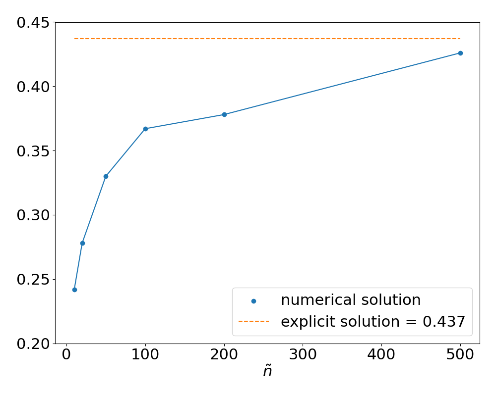
Figure 1: Numerical Implementation of [8] with delay = 0.7.

Acknowledgment The authors would like to thank Xavier Warin for providing the code in [34], and Huyên Pham for insightful discussions during his visit to U Michigan in April 2022.

References

- [1] Robert Azencott. Formule de Taylor stochastique et développements asymptotiques d’intégrales de Feynman In Azéma, Yor (Eds), Séminaire de probabilités, XVI, LNM921 237–284, Springer.
- [2] Imanol Perez Arribas. Derivatives pricing using signature payoffs. arXiv preprint arXiv:1809.09466, 2018.
- [3] Johan Auster, Ludovic Mathys, and Fabio Maeder. JDOI variance reduction method and the pricing of American-style options. Quantitative Finance, 22(4):639–656, 2022.
- [4] Fabrice Baudoin. An Introduction to the geometry of stochastic flows, Imperial College Press, 140 pp, 2005.
- [5] Fabrice Baudoin, Eulalia Nualart, Cheng Ouyang. and Samy Tindel. On probability laws of solutions to differential systems driven by a fractional Brownian motion. Ann. Probab. 44(2016), no.4, 2554–2590.
- [6] Fabrice Baudoin, Qi Feng, and Cheng Ouyang. Density of the signature process of fBm. Trans. Amer. Math. Soc. 373 (2020), no. 12, 8583-8610.
- [7] Jerome Barraquand and Thierry Pudet. Pricing of American path-dependent contingent claims. Mathematical Finance, 6(1):17–51, 1996.
- [8] Erhan Bayraktar and Zhou Zhou. On an Optimal Stopping Problem of an Insider. Theory of Probability & Its Applications, 61(2017), no. 1, 129-133.
- [9] Christian Bayer, Paul Hager, Sebastian Riedel, and John Schoenmakers. Optimal stopping with signatures. arXiv preprint arXiv:2105.00778, 2021.
- [10] Christian Bayer, Jinniao Qiu, and Yao Yao. Pricing options under rough volatility with backward SPDEs. SIAM Journal on Financial Mathematics, 13(1):179–212, 2022.
- [11] Erhan Bayraktar, Asaf Cohen, and April Nellis. A neural network approach to high-dimensional optimal switching problems with jumps in energy markets. arXiv preprint arXiv:2210.03045, 2022.
- [12] Sebastian Becker, Patrick Cheridito, and Arnulf Jentzen. Deep optimal stopping. The Journal of Machine Learning Research. 20.1 (2019): 2712-2736.
- [13] Sebastian Becker, Patrick Cheridito, and Arnulf Jentzen. Pricing and Hedging American-Style Options with Deep Learning Journal of Risk Financial Management. 2020, 13, 158. https://doi.org/10.3390/jrfm13070158.
- [14] Sebastian Becker, Patrick Cheridito, Arnulf Jentzen, and Timo Welti. Solving high-dimensional optimal stopping problems using deep learning. European Journal of Applied Mathematics, 32(3):470–514, 2021.
- [15] Cyril Benezet, Jean-Francois Chassagneux, and Adrien Richou. Switching problems with controlled randomisation and associated obliquely reflected BSDEs. Stochastic Processes and their Applications, 144:23–71, 2022.
- [16] Fabienne Castell. Asymptotic expansion of stochastic flows, Probab. Theory Relat. Fields (1993), 96, 225–239, .
- [17] René Carmona and Michael Ludkovski. Pricing asset scheduling flexibility using optimal switching. Applied Mathematical Finance, 15(5-6):405–447, 2008.
- [18] Jean-Francois Chassagneux and Adrien Richou. Rate of convergence for the discrete-time approximation of reflected BSDEs arising in switching problems. Stochastic Processes and their Applications, 129(11):4597–4637, 2019.
- [19] Kailin Ding, Zhenyu Cui, and Xiaoguang Yang. Pricing arithmetic Asian and Amerasian options: a diffusion operator integral expansion approach. Journal of Futures Markets, 2022, forthcoming.
- [20] Nicole El Karoui, Christophe Kapoudjian, Etienne Pardoux, Shige Peng, and Marie-Claire Quenez. Reflected solutions of backward SDE’s, and related obstacle problems for PDE’s. the Annals of Probability, 25(2):702–737, 1997.
- [21] Qi Feng and Xuejing Zhang. Taylor Expansions and Castell Estimates for Solutions of Stochastic Differential Equations Driven by Rough Paths. Journal of Stochastic Analysis: Vol. 1 : No. 2 , Article 4., 2020.
- [22] Qi Feng, Man Luo, and Zhaoyu Zhang. Deep signature FBSDE algorithm. Numerical Algebra, Control and Optimization, 2022.
- [23] Peter K. Friz and Nicolas B. Victoir Multidimensional stochastic processes as rough paths: theory and applications Cambridge University Press, vol 120, 2010.
- [24] Peter K Friz and Martin Hairer. A course on rough paths, Springer, 2020.
- [25] Ken-ichi Funahashi and Yuichi Nakamura. Approximation of dynamical systems by continuous time recurrent neural networks. Neural networks, 6(6):801–806, 1993.
- [26] Chengfan Gao, Siping Gao, Ruimeng Hu, and Zimu Zhu. Convergence of the backward deep BSDE method with applications to optimal stopping problems. arXiv preprint arXiv:2210.04118, 2022.
- [27] Lukas Gonon. Deep neural network expressivity for optimal stopping problems. arXiv preprint arXiv:2210.10443, 2022.
- [28] Said Hamadene and Jianfeng Zhang. Switching problem and related system of reflected backward SDEs. Stochastic Processes and their applications, 120(4):403–426, 2010.
- [29] Jiequn Han, Arnulf Jentzen, and Weinan E. Solving high-dimensional partial differential equations using deep learning. Proceedings of the National Academy of Sciences, 115(34):8505–8510, 2018.
- [30] Jiequn Han and Jihao Long. Convergence of the deep BSDE method for coupled FBSDEs. Probability, Uncertainty and Quantitative Risk, 5(1):1–33, 2020.
- [31] Asbjorn T Hansen and Peter Lochte Jorgensen. Analytical valuation of American-style Asian options. Management Science, 46(8):1116–1136, 2000.
- [32] Calypso Herrera, Florian Krach, Pierre Ruyssen, and Josef Teichmann. Optimal stopping via randomized neural networks. arXiv preprint arXiv:2104.13669, 2021.
- [33] Ying Hu, Remi Moreau, and Falei Wang. Mean-field reflected BSDEs: the general lipschitz case. arXiv preprint arXiv:2201.10359, 2022.
- [34] Côme Huré, Huyên Pham, and Xavier Warin. Deep backward schemes for high-dimensional nonlinear PDEs. Mathematics of Computation, 89(324):1547–1579, 2020.
- [35] Patrick Kidger, Patric Bonnier, Imanol Perez Arribas, Cristopher Salvi, and Terry Lyons. Deep signature transforms. In Advances in Neural Information Processing Systems, pages 3105–3115, 2019.
- [36] Jasdeep Kalsi, Terry Lyons and Imanol Perez Arribas Optimal Execution with Rough Path Signatures SIAM J. Financial Math., Vol. 11, No. 2, pages 470-493, 2020.
- [37] Terry Lyons and Zhongmin Qian. System control and rough paths. Oxford University Press, 2002.
- [38] Juan Li. Reflected mean-field backward stochastic differential equations. approximation and associated nonlinear PDEs. Journal of Mathematical Analysis and Applications, 413(1):47–68, 2014.
- [39] Jérôme Lelong. Pricing Path-Dependent Bermudan Options Using Wiener Chaos Expansion: An Embarrassingly Parallel Approach Journal of Computational Finance, Vol. 24, No. 2, 2019.
- [40] Bernard Lapeyre and Jérôme Lelong. Neural network regression for Bermudan option pricing Monte Carlo Methods and Applications, vol. 27, no. 3, 2021, pp. 227-247.
- [41] Francis A Longstaff and Eduardo S Schwartz. Valuing american options by simulation: a simple least-squares approach. The review of financial studies, 14(1):113–147, 2001.
- [42] Jin Ma and Jianfeng Zhang. Representations and regularities for solutions to BSDEs with reflections. Stochastic processes and their applications, 115(4):539–569, 2005.
- [43] Jean Mémin, Shi-ge Peng, and Ming-Yu Xu. Convergence of solutions of discrete reflected backward SDEs and simulations. Acta Mathematicae Applicatae Sinica, English Series, 24(1):1–18, 2008.
- [44] Eckhard Platen and Nicola Bruti-Liberati. Numerical solution of stochastic differential equations with jumps in finance, volume 64. Springer Science & Business Media, 2010.
- [45] Marc Sabate-Vidales, Daviv Siska, and Lukasz Szpruch. Solving path dependent PDEs with LSTM networks and path signatures. arXiv preprint, arXiv:2011.10630, 2020.
- [46] Johannes Schmidt-Hieber. Nonparametric regression using deep neural networks with ReLU activation function. Ann. Statist. 48(4): 1875-1897 (August 2020). DOI: 10.1214/19-AOS1875.
- [47] Haojie Wang, Han Chen, Agus Sudjianto, Richard Liu, and Qi Shen. Deep learning-based BSDE solver for LIBOR market model with application to Bermudan swaption pricing and hedging. arXiv preprint arXiv:1807.06622, 2018.
- [48] Yutian Wang and Yuan-Hua Ni. Deep BSDE-ML learning and its application to model-free optimal control. arXiv preprint arXiv:2201.01318, 2022.
- [49] Jianfeng Zhang. A numerical scheme for BSDEs. The Annals of Applied Probability, 14(1):459–488, 2004.