On-shell versus curvature mass parameter fixing schemes in the three flavor quark-meson model with vacuum fluctuations

Abstract

The vacuum effective potential and phase diagram for the three (2+1) flavor quark-meson model have been computed and compared in an extended mean-field approximation (e-MFA) where the model parameters are fixed by using different renormalization prescriptions after including quark one-loop vacuum fluctuations. When the vacuum one-loop divergence is regularized in the minimal subtraction scheme and the curvature masses of the scalar and pseudo-scalar mesons are used for fixing the parameters, the setting of the quark-meson model with the vacuum term (QMVT) turns out to be inconsistent as one notes that the curvature masses are defined by the evaluation of self-energy at zero momentum. This work constitutes the first application of the consistent on-shell parameter fixing scheme to the three flavor quark-meson (QM) model. In this setting of the renormalized quark-meson (RQM) model, the physical (pole) masses of the $\pi,K,\eta$ and $\eta^{\prime}$ pseudo-scalar mesons and the scalar $\sigma$ meson,the pion decay constant and kaon decay constant are put into the relation of the running mass parameter and couplings by using the on-shell and the minimal subtraction renormalization schemes. The nonstrange direction normalized vacuum effective potential plots for both the RQM model and QMVT model, are exactly identical for the $m_{\sigma}=$ 658.8 MeV while the nonstrange direction order parameter temperature variations and phase diagrams for both the models RQM and QMVT are identical when the $m_{\sigma}$ value is smaller by 10 MeV i.e. $m_{\sigma}=$ 648 MeV. This happens because the normalized vacuum effective potential variation in the nonstrange direction is somewhat influenced by its variation in the strange direction. When the $m_{\sigma}<$ 658.8 MeV, the nonstrange direction normalized vacuum effective potential is deepest for the QMVT model. One observes an interesting trend reversal for the $m_{\sigma}>$ 658.8 MeV when the nonstrange direction vacuum effective potential of the RQM model becomes deepest. Similar $m_{\sigma}$ dependent differences and similarities are noticed in the nature of the RQM and QMVT model phase diagrams and the nonstrange direction order parameter temperature variations. The normalized vacuum effective potential plots in the strange direction for both the RQM model and QMVT model, are nearly coincident for the $m_{\sigma}=$ 785 MeV. The effective potential variation in the strange direction for the $m_{\sigma}<$ 785 MeV is deepest in the QMVT model while for the $m_{\sigma}>$ 785 MeV, it becomes deepest for the RQM model.

1 Introduction

The study of quantum chromodynamics (QCD) phase diagram in all its details has been a very active research area of strong interaction physics since 1970s when the first QCD schematic phase diagram appeared Cabibbo75 . It depicted a confined phase of hadrons at a low temperature (low baryonic density) and a deconfined phase of quarks and gluons SveLer ; SveLer1 ; Mull ; Ortms ; Riske at a high temperature (zero baryonic density) or high baryonic density (zero temperature). One gets important and valuable information for the QCD phase transition from the lattice QCD simulations AliKhan:2001ek ; Digal:01 ; Karsch:02 ; Fodor:03 ; Allton:05 ; Karsch:05 ; Aoki:06 ; Cheng:06 ; Cheng:08 at zero chemical potential but for the non zero baryon densities/chemical potentials, the lattice QCD calculations get seriously compromised as the QCD action becomes complex on account of the fermion sign problem Karsch:02 . For mapping out the phase diagram regions where the lattice simulations do not work, one gets much help from the investigations carried out in the ambit of phenomenological models developed using the effective degrees of freedom Alf ; Fukhat .

In the zero quark mass limit, the QCD Lagrangian with the three flavor of quarks has the $SU_{L+R}(3)\times SU_{L-R}(3)$ symmetry. The axial ($A=L-R$) part of the symmetry is called the chiral symmetry. It gets spontaneously broken in the low energy hadronic vacuum of the QCD. This leads to the formation of chiral condensate and one gets eight massless pseudoscalar bosons as Goldstone bosons. The chiral symmetry gets explicitly broken as well due to the small mass of the light quarks $u,d$ and a relatively heavy $s$ quark. In the nature, we find light pions while kaons and eta are heavier due to the large mass of strange quark. Furthermore ’t Hooft tHooft:76prl ; tHooft:76prl1 showed that the $U_{A}(1)$ axial symmetry is explicitly broken to $Z_{A}(N_{f})$ at the quantum level by the instanton effects. Even in the chiral limit of zero quark masses, the $\eta^{\prime}$ meson is not a massless Goldstone boson as it acquires a mass of about 1 GeV due to the $U_{A}(1)$ axial anomaly. The framework of the three flavor linear sigma model Rischke:00 ; Rischke:001 ; Schaefer:09 is very conducive for investigating the $SU_{A}(3)$ chiral as well as the $U_{A}(1)$ axial symmetry breaking and restoration. It enables the construction of chiral invariant combinations using the chiral partners from the respective octet as well as the singlet of the scalar and pseudoscalar mesons. When the nine scalar and nine pseudo-scalar mesons are coupled to the three flavor of quarks, one gets the QCD-like framework of the quark-meson (QM) model for computing and exploring the QCD phase diagram.

Furthermore, the QCD confinement at low temperatures and densities is mimicked in a statistical sense by coupling the chiral models to a constant background $SU(N_{c})$ gauge field $A_{\mu}^{a}$ Polyakov:78plb ; fuku ; benji ; Pisarski:00prd ; Vkt:06 . Thus the confinement of quarks inside the hadrons gets implemented by the introduction of the Polyakov loop. When the free energy density from the gluons in the form of the phenomenological Polyakov loop potential ratti ; fuku2 is added to the QM model, one gets the PQM model. Different QCD phase structure/phase diagram studies, have already been done in the chiral models scav ; Roder ; fuku11 ; grahl ; jakobi ; Herpay:05 ; Herpay:06 ; Herpay:07 ; Kovacs:2006ym ; kahara ; kahara1 ; kahara2 ; Bowman:2008kc ; Bowman:2008kc1 ; Fejos ; Jakovac:2010uy ; koch ; marko , two and three flavor QM model mocsy ; bj ; Schaefer:2006ds and PQM model SchaPQM2F ; SchaPQM3F ; Mao ; TiPQM3F .

The quark one-loop vacuum fluctuations and the associated renormalization issues are neglected altogether scav ; mocsy ; bj ; Schaefer:2006ds ; SchaPQM2F ; kahara ; kahara1 ; kahara2 ; Schaefer:09 ; SchaPQM3F ; Mao ; TiPQM3F in the QM model with the standard mean field approximation (s-MFA) under the assumption that the redefinition of the meson potential parameters would account for their effects. The QM model in the chiral limit under the s-MFA, gives a first-order chiral phase transition at zero baryon densities. This result is inconsistent because the general theoretical arguments rob ; hjss predict that the abovementioned chiral phase transition should be of second order. In order to remedy the inconsistency, proper treatment of the Dirac sea was first proposed in the Ref. vac . Afterwards, the quark one-loop vacuum corrections were included in the two and three flavor QM/PQM models and its detailed impact on the phase diagram and phase structure was investigated in several research papers lars ; guptiw ; schafwag12 ; chatmoh1 ; TranAnd ; vkkr12 ; chatmoh2 ; vkkt13 ; Herbst ; Weyrich ; kovacs ; zacchi1 ; zacchi2 ; Rai . For the fixing of the model parameters, these publications have used the curvature masses of the mesons while the pion decay constant is identified with the vacuum expectation value of the sigma mean field. In the three flavor QM/PQM model with fermionic vacuum correction schafwag12 ; chatmoh1 ; chatmoh2 ; vkkt13 ; Rai , one has the kaon decay constant also which is given by the combination of the vacuum expectation values of the strange and nonstrange condensate. The quark one-loop vacuum divergence in the abovementioned works has been properly regularized by using the minimal subtraction scheme. The curvature mass is akin to defining the meson mass by the evaluation of self-energy at zero momentum because the effective potential is the generator of the n-point functions of the theory at vanishing external momenta laine ; Adhiand1 ; BubaCar ; Naylor ; fix1 . This consideration makes the above parameter fixing procedure inconsistent. For making comparisons and quantifying the effect of the parameter fixing with the curvature meson masses, this model setting has been named as the quark-meson model with vacuum term (QMVT).

The radiative corrections to the physical quantities in most of the renormalization procedures, change their tree level relations to the parameters of the Lagrangian. Thus the effective potential calculation becomes inconsistent if one uses the tree level values of the parameters. The on-shell parameters have their tree-level values while the running parameters in the $\overline{\text{MS}}$ scheme depend on the renormalization scale $\Lambda$. According to the correct renormalization prescription, one needs to calculate the counterterms both in the $\overline{\text{MS}}$ scheme and in the on-shell scheme and then connect the renormalized parameters of the two schemes. Afterwards the effective potential is calculated using the modified minimal subtraction procedure where the relations between the on-shell parameters (physical quantities) and the running parameters are used as the input Adhiand1 . In a series of papers, Adhikari and collaborators Adhiand1 ; Adhiand2 ; Adhiand3 ; asmuAnd have used this renormalization prescription for the proper accounting of the effect of Dirac sea in the context of two flavor QM model which uses the $O(4)$ sigma model with the iso-singlet scalar $\sigma$ and the iso-triplet pseudoscalar $\pi$ meson.

In a very recent research work, we have also applied RaiTiw the on-shell parameter fixing scheme to that version of the quark-meson (QM) model in which the two flavor of quarks are coupled to the eight mesons of the $SU_{L}(2)\times SU_{R}(2)$ linear sigma model and then made a comparative study of the effective potentials as well as the phase diagrams when the QM model setting with the on-shell parameters is contrasted with QM model parameter fixing using the curvature masses. In the present work, we will apply the on-shell parameter fixing scheme to the three (2+1) flavor quark-meson (QM) model in which the three flavor of quarks are coupled to the octect and singlet scalar as well as pseudoscalar mesons of the $SU_{L}(3)\times SU_{R}(3)$ linear sigma model. This model setting has been termed as the renormalized quark-meson (RQM) model which has the advantage of providing us the framework in which apart from the $SU_{A}(3)$ chiral, we can investigate the $U_{A}(1)$ axial symmetry breaking and restoration also together with the interplay of axial $U_{A}(1)$ and $SU_{A}(3)$ chiral symmetry.

The paper is arranged as follows. The brief formulation of the $SU_{L}(3)\times SU_{R}(3)$ QM model is presented in the section 2. The section 3 presents the calculation of the effective potential of the quark-meson model with vacuum term (QMVT) together with its parameter fixing procedure which uses the curvature masses of the scalar and pseudo-scalar mesons. The on-shell scheme counterterms and self-energy calculations are presented in the section 4.1. The relations between the physical quantities and the running parameters, are derived in the section 4.2, the derivation of the effective potential in the RQM model is presented in the section 4.3. The result and discussion is presented in the section 5. Finally summary and conclusion is presented in the section 6.

2 Model Formulation

We are presenting the formulation of the $SU_{L}(3)\times SU_{R}(3)$ quark-meson model in this section. Three flavor of quarks in this model are coupled to the $SU_{V}(3)\times SU_{A}(3)$ symmetric meson fields. The model Lagrangian is written in terms of quarks, mesons and couplings as

$${\cal L_{QM}} = \bar{\psi}[i\gamma^{\mu}\partial_{\mu}-g\;T_{a}\big{(}\sigma_{a}+i\gamma_{5}\pi_{a}\big{)}]\psi+\cal{L(M)},$$ (1)

where $\psi$ is a color $N_{c}$-plet, a four-component Dirac spinor as well as a flavor triplet

$$\psi = \left(\begin{array}[]{c}u\\ d\\ s\end{array}\right)\;.$$ (5)

The flavor blind Yukawa coupling $g$ couples the three flavor of quarks with the nine scalar ($\sigma_{a},J^{P}=0^{+}$) and nine pseudoscalar ($\pi_{a},J^{P}=0^{-}$) mesons. The massless quarks become massive due to the spontaneous breaking of the chiral symmetry as the chiral condensate assumes non-zero vacuum expectation value. The Lagrangian for the meson fields has the following form Schaefer:09 ; Roder ; TiPQM3F

$$\cal{L(M)} = \text{Tr}(\partial_{\mu}{\cal{M}}^{\dagger}\partial^{\mu}{\cal{M}}-m^{2}({\cal{M}}^{\dagger}{\cal{M}}))$$ (6)

$$-\lambda_{1}\left[\text{Tr}({\cal{M}}^{\dagger}{\cal{M}})\right]^{2}-\lambda_{2}\text{Tr}({\cal{M}}^{\dagger}{\cal{M}})^{2}$$

$$+c[\text{det}{\cal{M}}+\text{det}{\cal{M}}^{\dagger}]+\text{Tr}\left[H({\cal{M}}+{\cal{M}}^{\dagger})\right]\;,$$

here the field ${\cal{M}}$ is a complex $3\times 3$ matrix which contains the nine scalars $\sigma_{a}$ and the nine pseudoscalar $\pi_{a}$ mesons.

$${\cal{M}} = T_{a}\xi_{a}=T_{a}(\sigma_{a}+i\pi_{a})\;.$$ (7)

Here the $T_{a}$ represent 9 generators of $U(3)$ with $T_{a}=\frac{\lambda_{a}}{2}$ where $a=0,1,\dots~{},8$. The $\lambda_{a}$ are standard Gell-Mann matrices with $\lambda_{0}=\sqrt{\frac{2}{3}}\ {\mathbb{I}}_{3\times 3}$. The generators follow the $U(3)$ algebra $\left[T_{a},T_{b}\right]=if_{abc}T_{c}$ and $\left\{T_{a},T_{b}\right\}=d_{abc}T_{c}$ where $f_{abc}$ and $d_{abc}$ are the standard antisymmetric and symmetric structure constants respectively with $f_{ab0}=0$ and $d_{ab0}=\sqrt{\frac{2}{3}}\ \delta_{ab}$ and matrices are normalized as $\text{Tr}(T_{a}T_{b})=\frac{\delta_{ab}}{2}$. The following term breaks the $SU_{L}(3)\times SU_{R}(3)$ chiral symmetry explicitly.

$$H=T_{a}h_{a}\;.$$ (8)

Here $H$ is a $3\times 3$ matrix with nine external parameters. On account of the spontaneous breaking of the chiral symmetry, the filed $\xi$ picks up the nonzero vacuum expectation value, $\bar{\xi}$. Only three possible nonzero parameters $h_{0}$, $h_{3}$ and $h_{8}$ might cause the explicit breakdown of the chiral symmetry because $\bar{\xi}$ must have the quantum numbers of the vacuum. We are choosing $h_{0}$, $h_{8}\neq 0$ and isospin symmetry breaking is neglected. Thus having the nonzero condensates $\bar{\sigma_{0}}$ and $\bar{\sigma_{8}}$, one gets the $2+1$ flavor symmetry breaking scenario. The model has five other parameters in addition to the $h_{0}$ and $h_{8}$. These are the tree-level mass parameter squared $m^{2}$, quartic coupling constants $\lambda_{1}$ and $\lambda_{2}$, a Yukawa coupling $g$ and a cubic coupling constant $c$ which models the $U_{A}(1)$ axial anomaly of the QCD vacuum.

Table 1: Meson masses calculated from the second derivative of the grand potential at its minimum as given in Ref. Schaefer:09 ; Herpay:06

	Scalar meson masses		Pseudo-scalar meson masses
$(m_{a_{0}})^{2}$	$m^{2}+\lambda_{1}(x^{2}+y^{2})+\frac{3\lambda_{2}}{2}x^{2}+\frac{\sqrt{2}c}{2}y$	$(m_{\pi})^{2}$	$m^{2}+\lambda_{1}(x^{2}+y^{2})+\frac{\lambda_{2}}{2}x^{2}-\frac{\sqrt{2}c}{2}y$
$(m_{\kappa})^{2}$	$m^{2}+\lambda_{1}(x^{2}+y^{2})+\frac{\lambda_{2}}{2}(x^{2}+\sqrt{2}xy+2y^{2})+\frac{c}{2}x$	$(m_{K})^{2}$	$m^{2}+\lambda_{1}(x^{2}+y^{2})+\frac{\lambda_{2}}{2}(x^{2}-\sqrt{2}xy+2y^{2})-\frac{c}{2}x$
$(m_{s,00})^{2}$	$m^{2}+\frac{\lambda_{1}}{3}(7x^{2}+4\sqrt{2}xy+5y^{2})+\lambda_{2}(x^{2}+y^{2})-\frac{\sqrt{2}c}{3}(\sqrt{2}x+y)$	$(m_{p,00})^{2}$	$m^{2}+\lambda_{1}(x^{2}+y^{2})+\frac{\lambda_{2}}{3}(x^{2}+y^{2})+\frac{c}{3}(2x+\sqrt{2}y)$
$(m_{s,88})^{2}$	$m^{2}+\frac{\lambda_{1}}{3}(5x^{2}-4\sqrt{2}xy+7y^{2})+\lambda_{2}(\frac{x^{2}}{2}+2y^{2})+\frac{\sqrt{2}c}{3}(\sqrt{2}x-\frac{y}{2})$	$(m_{p,88})^{2}$	$m^{2}+\lambda_{1}(x^{2}+y^{2})+\frac{\lambda_{2}}{6}(x^{2}+4y^{2})-\frac{c}{6}(4x-\sqrt{2}y)$
$(m_{s,08})^{2}$	$\frac{2\lambda_{1}}{3}(\sqrt{2}x^{2}-xy-\sqrt{2}y^{2})+\sqrt{2}\lambda_{2}(\frac{x^{2}}{2}-y^{2})+\frac{c}{3\sqrt{2}}(x-\sqrt{2}y)$	$(m_{p,08})^{2}$	$\frac{\sqrt{2}\lambda_{2}}{6}(x^{2}-2y^{2})-\frac{c}{6}(\sqrt{2}x-2y)$
$(m_{s,xx})^{2}$	$m^{2}+3(\lambda_{1}+\frac{\lambda_{2}}{2})x^{2}+\lambda_{1}y^{2}-\frac{c}{\sqrt{2}}y$	$(m_{p,xx})^{2}$	$m^{2}+(\lambda_{1}+\frac{\lambda_{2}}{2})x^{2}+\lambda_{1}y^{2}+\frac{c}{\sqrt{2}}y$
$(m_{s,yy})^{2}$	$m^{2}+\lambda_{1}x^{2}+3(\lambda_{1}+\lambda_{2})y^{2}$	$(m_{p,yy})^{2}$	$m^{2}+\lambda_{1}x^{2}+(\lambda_{1}+\lambda_{2})y^{2}$
$(m_{s,xy})^{2}$	$2\lambda_{1}xy-\frac{c}{\sqrt{2}}x$	$(m_{p,xy})^{2}$	$\frac{c}{\sqrt{2}}x$
$m_{\sigma}^{2}$	$\frac{1}{2}(m_{s,00}^{2}+m_{s,88}^{2})$	$m_{\eta}^{2}$	$\frac{1}{2}(m_{p,00}^{2}+m_{p,88}^{2})$
	$-\frac{1}{2}\sqrt{(m_{s,00}^{2}-m_{s,88}^{2})^{2}+4m_{s,00}^{4}}$		$-\frac{1}{2}\sqrt{(m_{p,00}^{2}-m_{p,88}^{2})^{2}+4m_{p,00}^{4}}$
$m_{f_{0}}^{2}$	$\frac{1}{2}(m_{s,00}^{2}+m_{s,88}^{2})$	$m_{\eta^{\prime}}^{2}$	$\frac{1}{2}(m_{p,00}^{2}+m_{p,88}^{2})$
	$+\frac{1}{2}\sqrt{(m_{s,00}^{2}-m_{s,88}^{2})^{2}+4m_{s,00}^{4}}$		$+\frac{1}{2}\sqrt{(m_{p,00}^{2}-m_{p,88}^{2})^{2}+4m_{p,00}^{4}}$

2.1 Grand Potential in the Mean Field Approach

The considered system is spatially uniform and it is in thermal equilibrium at temperature $T$ and quark chemical potential $\mu_{f}(f=u,d,s)$. The partition function is obtained by the path integral over the quark/antiquark and meson fields Schaefer:09 ; TiPQM3F

$$\mathcal{Z} = \mathrm{Tr\,exp}[-\beta(\hat{\mathcal{H}}-\sum_{f=u,d,s}\mu_{f}\hat{\mathcal{N}}_{f})]$$ (9)

$$= \int\prod_{a}\mathcal{D}\sigma_{a}\mathcal{D}\pi_{a}\int\mathcal{D}\psi\mathcal{D}\bar{\psi}\;\mathrm{exp}\bigg{[}-\int_{0}^{\beta}d\tau\int_{V}d^{3}x$$

$$\bigg{(}\mathcal{L_{QM}^{E}}+\sum_{f=u,d,s}\mu_{f}\bar{\psi}_{f}\gamma^{0}\psi_{f}\bigg{)}\bigg{]}\;.$$

Where $\beta=\frac{1}{T}$ and the three dimensional volume of the system is $V$. In general, the three quark chemical potentials will be different for the three quark flavors. It is assumed that the $SU_{V}(2)$ symmetry is preserved in this work. Hence the small difference in the mass of $u$ and $d$ quark is neglected. Thus the quark chemical potential for the $u$ and $d$ quarks is equal $\mu_{u}=\mu_{d}$ and the strange quark chemical potential is $\mu_{s}$.

In the standard mean-field approximation scav ; Schaefer:09 ; TiPQM3F , the partition function is calculated by replacing the meson fields with their vacuum expectation values $\langle M\rangle=T_{0}\bar{\sigma_{0}}+T_{8}\bar{\sigma_{8}}$ and neglecting the thermal as well as quantum fluctuations of the meson fields while retaining the quarks and antiquarks as quantum fields. Using the standard method given in Refs. fuku ; SchaPQM2F ; Kapusta_Gale , one can find the expression of grand potential as the sum of meson and quark/antiquark contribution,

$$\Omega_{\rm MF}(T,\mu)=-\frac{T\ln Z}{V} = U(\sigma_{0},\sigma_{8})+\Omega_{\bar{q}q}(T,\mu)\;.$$ (10)

The 2 + 1 flavor case is studied by performing the following basis transformation of condensates and external fields from the original singlet octet (0, 8) basis to the nonstrange strange basis ($x$, $y$)

$$\sigma_{x} = x=\sqrt{\frac{2}{3}}\bar{\sigma}_{0}+\frac{1}{\sqrt{3}}\bar{\sigma}_{8},$$ (11)

$$\sigma_{y} = y=\frac{1}{\sqrt{3}}\bar{\sigma}_{0}-\sqrt{\frac{2}{3}}\bar{\sigma}_{8}.$$ (12)

The grand potential is written in $x$, $y$ basis as,

$$\Omega_{\rm MF}(T,\mu)=U(x,y)+\Omega_{q\bar{q}}(T,\mu)\;.$$ (13)

The external fields ($h_{x}$, $h_{y}$) are written in terms of the ($h_{0}$, $h_{8}$) by similar expressions. Since the nonstrange and strange quark/antiquark decouple, the quark masses are written as,

$$m_{u}=g\frac{x}{2},\qquad m_{s}=g\frac{y}{\sqrt{2}}\;.$$ (14)

The tree level effective potential in the nonstrange-strange basis is written as,

$$U(x,y) = \frac{m^{2}}{2}\left(x^{2}+y^{2}\right)-h_{x}x-h_{y}y-\frac{c}{2\sqrt{2}}x^{2}y$$ (15)

$$+\frac{\lambda_{1}}{2}x^{2}y^{2}+\frac{1}{8}\left(2\lambda_{1}+\lambda_{2}\right)x^{4}$$

$$+\frac{1}{8}\left(2\lambda_{1}+2\lambda_{2}\right)y^{4}\ ,$$

The stationarity conditions $\frac{\partial U(x,y)}{\partial x}|_{x=\overline{x},y=\overline{y}}=0=\frac{\partial U(x,y)}{\partial y}|_{x=\overline{x},y=\overline{y}}$ for the effective potential (15) give

$${\hskip-21.33955pt}h_{x} = \overline{x}\ m^{2}_{\pi}\ \text{and}\ h_{y}={\biggl{\{}\frac{\sqrt{2}}{2}(m_{K}^{2}-m_{\pi}^{2})\overline{x}+m_{K}^{2}\overline{y}\biggr{\}}}\;.\quad$$ (16)

The tree level curvature masses of the pions, kaons and other mesons in the QM model are given by the mass matrix $(m_{\alpha,ab})^{2}$ evaluated in Ref. Rischke:00 ; Rischke:001 ; Schaefer:09 . Here $\alpha=$ s, p; “s” stands for the scalar and “p” stands for the pseudoscalar mesons and $a,b=0,1,2,\cdots,8$. In the scalar sector, the $a_{0}$ meson mass is given by the 11 element (degenerate with the 22 and 33 elements) and the $\kappa$ meson mass is given by the 44 element (degenerate with the 55, 66 and 77 elements). The $\sigma$ and $f_{0}$ meson masses are found by diagonalizing the (00)-(88) sector of the scalar mass matrix. In exactly analogous manner for the pseudoscalar sector $m^{2}_{\text{p},11}=m^{2}_{\text{p},22}=m^{2}_{\text{p},33}\equiv m^{2}_{\pi}$ and $m^{2}_{\text{p},44}=m^{2}_{\text{p},55}=m^{2}_{\text{p},66}=m^{2}_{\text{p},77}\equiv m^{2}_{K}$. Diagonalization of the pseudoscalar (00)-(88) sector of the mass matrix gives us the masses of the physical $\eta$ and $\eta^{\prime}$ mesons. All the meson masses are given in the Table 1.

The quark/antiquark contribution is given by,

$$\Omega_{q\bar{q}}(T,\mu;x,y) = \Omega_{q\bar{q}}^{vac}+\Omega_{q\bar{q}}^{T,\mu}\;,$$ (17)

$$\Omega_{q\bar{q}}^{vac} = -2N_{c}\sum_{u,d,s}\int\frac{d^{3}p}{(2\pi)^{3}}E_{f}\theta(\Lambda_{c}^{2}-\vec{p}^{2})\;,$$ (18)

$$\Omega_{q\bar{q}}^{T,\mu} = -2N_{c}\sum_{u,d,s}\int\frac{d^{3}p}{(2\pi)^{3}}T\left[\ln\left(1+e^{-E_{f}^{+}/T}\right)+\ln\left(1+e^{-E_{f}^{-}/T}\right)\right]\;.$$ (19)

The fermion vacuum contribution is given by the first term of the Eq. (17), where $\Lambda_{c}$ is the ultraviolet cutoff. $E_{f}^{\pm}=E_{f}\mp\mu_{f}$ and $E_{f}=\sqrt{p^{2}+m{{}_{f}}{{}^{2}}}$ is the flavor dependent single particle energy of the quark/antiquark, $m_{u}=m_{d}=\frac{gx}{2}$ is the mass of the light quarks $u$, $d$ and strange quark mass is $m_{s}=\frac{gy}{\sqrt{2}}$. For the present work, it is assumed that $\mu_{u}=\mu_{d}=\mu_{s}=\mu$.

In the standard mean-field approximation (s-MFA), the quark one-loop vacuum term of the Eq. (17) is neglected and the QM model grand potential is written as,

$$\Omega_{QM}(T,\mu,x,y) = U(x,y)+\Omega_{q\bar{q}}^{T,\mu}\;.$$ (20)

The chiral order parameters $x$ for the nonstrange and $y$ for the strange sector are obtained by minimizing the thermodynamic potential the Eq. (20) in the nonstrange and strange directions

$$\frac{\partial\Omega_{QM}(T,\mu,x,y)}{\partial x}|_{x,y}=\frac{\partial\Omega_{QM}(T,\mu,x,y)}{\partial y}|_{x,y}=0.$$ (21)

2.2 Parameter fixing

The six model parameters $m^{2}$, $\lambda_{1}$, $\lambda_{2}$, $c$, $h_{x}$ and $h_{y}$ are obtained using six experimentally known quantities in the vacuum. The pion, kaon mass, the average squared mass of the $\eta$ and $\eta^{\prime}$ mesons ($m_{\eta}^{2}+m_{\eta^{\prime}}^{2}$) from the pseudo-scalar side and the mass $m_{\sigma}$ of the scalar meson $\sigma$ together with the pion and kaon decay constants $f_{\pi}$ and $f_{K}$ are used as the input Rischke:00 ; Rischke:001 ; Schaefer:09 for determining the six model parameters.

In accordance of the partially conserved axial-vector current relation (PCAC), the vacuum condensates values are $\overline{x}=f_{\pi}$ and $\overline{y}=(2f_{K}-f_{\pi})/\sqrt{2}$. The minimum of the effective potential in the Eq. (21) for $T=0,\mu=0$ is located at the above values. The parameters $\lambda_{2}$ and $c$ in the vacuum are obtained as

$$\lambda_{2} = \dfrac{2\ }{(x^{2}+4y^{2})(\sqrt{2}\ y-x)}\left[(3\sqrt{2}\ y)m_{K}^{2}-(\sqrt{2}y+2x)m_{\pi}^{2}-(\sqrt{2}y-x)(m_{\eta}^{2}+m_{\eta^{{}^{\prime}}}^{2})\right]\;,\hskip 22.76228pt$$ (22)

$$c = \dfrac{2(m^{2}_{K}-m^{2}_{\pi})}{(\sqrt{2}\ y-x)}-\sqrt{2}\ y\ \lambda_{2}\;.$$ (23)

The difference of the $\sigma$ and $\pi$ mass squares $(m_{\sigma}^{2}-m_{\pi}^{2})$ does not have any mass parameter $m^{2}$ dependence. It depends on the parameters $\lambda_{1}$, $\lambda_{2}$ and $c$. When the $\lambda_{2}$ and $c$ as obtained from the above two equations are put into the expression of $(m_{\sigma}^{2}-m_{\pi}^{2})$ and $x=\overline{x}=f_{\pi}$ and $y=\overline{y}=(2f_{K}-f_{\pi})/\sqrt{2}$, one gets the vacuum value of the parameter $\lambda_{1}$. Using the expression of $m_{\pi}^{2}$, the mass parameter $m^{2}$ can be written as

$$m^{2} = m^{2}_{\pi}-\lambda_{1}(x^{2}+y^{2})-\frac{\lambda_{2}}{2}x^{2}+\frac{c}{\sqrt{2}}y\;.$$ (24)

Putting the vacuum values of $m_{\pi}^{2}$, $\lambda_{1}$, $\lambda_{2}$, $c$, $x$ and $y$ in the Eq. (24), one gets the value of the mass parameter $m^{2}$. Putting the $\overline{x}$ and $\overline{y}$ values in the Eq. (16), one gets

$$h_{x} = f_{\pi}m^{2}_{\pi}\ \text{and}\ h_{y}=\sqrt{2}f_{K}\ m_{K}^{2}-\frac{1}{\sqrt{2}}f_{\pi}\ m_{\pi}^{2}\;.$$ (25)

Finally, the Yukawa coupling is fixed from the nonstrange constituent quark mass $g=\frac{2m_{u}}{f_{\pi}}$. For the $f_{\pi}=92.4$ MeV and $m_{u}\sim 300.3$ MeV, the $g\sim 6.5$ and strange quark mass is predicted to be $m_{s}\sim 334.34$ MeV. The experimental value of $m_{\eta}=547.5$ MeV and $m_{\eta^{\prime}}=957.78$ MeV. In Ref. Schaefer:09 , the parameter $\lambda_{2}$ is determined by taking the $m_{\eta}=539$ MeV and $m_{\eta^{\prime}}=963$ MeV as input because the sum of the squared masses $m_{\eta}^{2}+m_{\eta^{\prime}}^{2}=(539)^{2}+(963)^{2}$ is almost equal to the $(547.5)^{2}+(957.78)^{2}$ and the calculated parameters reproduce $m_{\eta}=539$ MeV and $m_{\eta^{\prime}}=963$ MeV in the output.

3 QM Model with Vacuum Term

This section contains a brief description of the effective potential calculation when the scalar and pseudo-scalar mesons curvature masses are used for the parameter fixing and the vacuum value of the nonstrange condensate is put equal to the pion decay constant while the strange condensate vacuum value is a combination of the pion and kaon decay constant. The quark one-loop vacuum divergence given by the first term of the Eq. (17) is regularized under the minimal subtraction scheme using the dimensional regularization as done for the two flavor case in Ref. vac ; guptiw ; vkkr12 and the three flavor case in Ref. schafwag12 ; chatmoh1 ; chatmoh2 ; vkkt13 . The quark one-loop vacuum term is written as

$$\Omega_{q\bar{q}}^{\rm vac} = -2N_{c}\sum_{f=u,d,s}\int\frac{d^{3}p}{(2\pi)^{3}}E_{f}\;.$$ (26)

The dimensional regularization of the Eq. (26) near three dimensions, $d=3-2\epsilon$ yields the $\epsilon$ zeroth order potential as

$${\hskip-2.84544pt}\Omega_{q\bar{q}}^{\rm vac}=\sum_{f=u,d,s}\frac{N_{c}\ m_{f}^{4}}{16\pi^{2}}\left[\frac{1}{\epsilon}-\frac{\{-3+2\gamma_{E}+4\ln(\frac{m_{f}}{2\sqrt{\pi}\Lambda})\}}{2}\right],$$ (27)

Here $\Lambda$ is the arbitrary renormalization scale. When the following counter term $\delta\mathcal{L}$ is added to the QM model Lagrangian,

$$\delta\mathcal{L}=\sum_{f=u,d,s}\frac{N_{c}}{16\pi^{2}}m_{f}^{4}\left[\frac{1}{\epsilon}-\frac{1}{2}\left\{-3+2\gamma_{E}-4\ln(2\sqrt{\pi})\right\}\right],$$ (28)

one gets the renormalized fermion vacuum loop contribution as:

$$\Omega_{q\bar{q}}^{\rm vac}=-\sum_{f=u,d,s}\frac{N_{c}}{8\pi^{2}}m_{f}^{4}\ln\left(\frac{m_{f}}{\Lambda}\right)\;,$$ (29)

The vacuum grand potential becomes the renormalization scale $\Lambda$ dependent when the quark one-loop contribution in the first term of the Eq. (17) is replaced by the Eq. (29) and one writes :

$$\Omega^{\Lambda}(x,y)=U(x,y)+\Omega_{q\bar{q}}^{\rm vac}$$ (30)

Here the six unknown parameters $m^{2}$, $\lambda_{1},\lambda_{2}$, $h_{x},h_{y}$ and $c$ of the meson potential U($x,y$), are obtained from the $x$ and $y$ dependent curvature masses of the mesons. The procedural details of finding the different parameters are presented in the Appendix (A). When the parameter $\lambda_{2}$ is determined, the logarithmic $\Lambda$ dependence in the term $\Omega_{q\bar{q}}^{\rm vac}$ generates a renormalization scale $\Lambda$ dependent part $\lambda_{2\Lambda}$ and one gets $\lambda_{2}=\lambda_{2s}+n+\lambda_{2+}+\lambda_{2\Lambda}$. $\lambda_{2s}$ is the same old $\lambda_{2}$ parameter of the QM/PQM model in the Ref. Rischke:00 ; Rischke:001 ; Schaefer:09 ; TiPQM3F . Here, $n=\frac{N_{c}g^{4}}{32\pi^{2}}$, $\lambda_{2+}=\frac{n{f_{\pi}}^{2}}{f_{K}\left(f_{K}-f_{\pi}\right)}\log\{\frac{2f_{K}-f_{\pi}}{f_{\pi}}\}$ and $\lambda_{2\Lambda}=4n\log\{\frac{g\left(2f_{K}-f_{\pi}\right)}{2\Lambda}\}$. When this value of the $\lambda_{2}$ is substituted in the expression of U($x,y$) and all the terms of the summation in $\Omega_{q\bar{q}}^{\rm vac}$ expression are written explicitly, the Eq. (30) takes the form :

$${\hskip-28.45274pt}\Omega^{\Lambda}(x,y) = \frac{m^{2}}{2}\left(x^{2}+y^{2}\right)-h_{x}x-h_{y}y-\frac{c}{2\sqrt{2}}x^{2}y+\frac{\lambda_{1}}{4}\left(x^{4}+y^{4}+2x^{2}y^{2}\right)$$ (31)

$$+\frac{\left(\lambda_{2\text{v}}+n+\lambda_{2\Lambda}\right)}{8}\left(x^{4}+2y^{4}\right)-\frac{nx^{4}}{2}\log\left(\frac{g\ x}{2\Lambda}\right)-\ ny^{4}\log\left(\frac{g\ y}{\sqrt{2}\Lambda}\right)\;.$$

The $\lambda_{2\text{v}}=\lambda_{2s}+\lambda_{2+}$. When the terms are rearranged, one finds that the scale dependence of all the terms in $\Omega_{q\bar{q}}^{\rm vac}$ gets completely cancelled by the logarithmic $\Lambda$ dependence of the $\lambda_{2}$ contained in $\lambda_{2\Lambda}$. The scale independent vacuum effective potential expression is

$${\hskip-28.45274pt}\Omega(x,y) = \frac{m^{2}}{2}\left(x^{2}+y^{2}\right)-h_{x}x-h_{y}y-\frac{c}{2\sqrt{2}}x^{2}y+\frac{\lambda_{1}}{4}\left(x^{4}+y^{4}+2x^{2}y^{2}\right)$$ (32)

$$+\frac{\left(\lambda_{2\text{v}}+n\right)}{8}\left(x^{4}+2y^{4}\right)-\frac{nx^{4}}{2}\log\left(\frac{x}{\left(2f_{K}-f_{\pi}\right)}\right)-ny^{4}\log\left(\frac{\sqrt{2}\ y}{\left(2f_{K}-f_{\pi}\right)}\right)\;.$$

One notes that the parameters $m^{2}$, $\lambda_{1}$ and $\lambda_{2}$ are modified by the fermionic vacuum correction in this parameter fixing scheme while the parameters $h_{x}$, $h_{y}$ and $c$ are not affected.

The thermodynamic grand potential with the renormalized fermionic vacuum correction in the quark meson model with vacuum term (QMVT) is written as

$$\Omega_{\rm QMVT}(T,\mu;x,y) = \Omega(x,y)+\Omega_{q\bar{q}}^{\rm T}(T,\mu;x,y)\;.$$ (33)

The nonstrange and strange quark condensates $x$ and $y$ are found by searching the global minimum of the grand potential for a given temperature $T$ and chemical potential $\mu$.

$$\frac{\partial\Omega_{\rm QMVT}(T,\mu;x,y)}{\partial x}|_{x,y} = \frac{\partial\Omega_{\rm QMVT}(T,\mu;x,y)}{\partial y}|_{x,y}=0$$

. (34)

Here it is relevant to remind that the dressing of the meson propagator is not considered in the curvature mass scheme of parameter fixing. Hence the pion and kaon decay constants $f_{\pi}$ and $f_{K}$ do not get renormalized. The quark one-loop vacuum correction to the effective potential modifies the parameters in such a way that the stationarity conditions in the nonstrange and strange directions for the $T=0$ give the same result for $h_{x}$ and $h_{y}$ as in the QM model. The modified curvature masses of the pion and kaon as presented in the Appendix (B) of Ref. vkkt13 remain the same as their pole masses. The minimum of the vacuum effective potential remains at $\overline{x}=f_{\pi}$ and $\overline{y}=\frac{2f_{K}-f_{\pi})}{\sqrt{2}}$.

4 Renormalized Quark Meson Model

Model parameters in several of the recent research works were fixed by taking the $\pi,K,\eta,\eta^{\prime}$ and $\sigma$ meson masses equal to the their curvature (or screening) masses lars ; guptiw ; schafwag12 ; chatmoh1 ; TranAnd ; vkkr12 ; chatmoh2 ; vkkt13 ; Herbst ; Weyrich ; kovacs ; zacchi1 ; zacchi2 ; Rai while the nonstrange condensate is put equal to the pion decay constant and the strange condensate is related to the pion and kaon decay constant. However, we know that the poles of the meson propagators give their physical masses and the residue of the pion propagator at its pole is related to the pion decay constant BubaCar ; Naylor ; fix1 . Furthermore, the curvature masses are akin to defining the meson masses by evaluating their self-energies at zero momentum laine ; Adhiand1 ; Adhiand2 ; Adhiand3 as it is known that the effective potential is the generator of the n-point functions of the theory at zero external momenta. It is also to be noted that the pole definition is the physical and gauge invariant one Kobes ; Kobes1 ; Rebhan . In the absence of the Dirac sea contributions, the pole mass prescription is equivalent to the curvature mass prescription for the parameter fixing of the model but when the quark one-loop vacuum correction is taken into account, the pole masses of the mesons start to differ from their screening masses BubaCar ; fix1 . The above arguments necessitate the use of the exact on-shell parameter fixing method for the renormalized quark-meson (RQM) model where the physical (pole) masses of the mesons, the pion and kaon decay constants are put into the relation of the running mass parameter and couplings by using the on-shell and the minimal subtraction renormalization prescriptions Adhiand2 ; asmuAnd ; RaiTiw .

4.1 Self-energies and counterterms

When the quark one-loop vacuum corrections are included, the tree level parameters of the Eqs. (22)–(25) become inconsistent unless one uses the on-shell renormalization scheme. The divergent loop integrals in the on-shell scheme are also regularized by the dimensional regularization but the counterterm choices are different from the minimal subtraction scheme. The suitable choice of counterterms in the on-shell scheme leads to the exact cancellation of the loop corrections to the self-energies. Since the couplings are evaluated on-shell, the renormalized parameters become renormalization scale independent. The parameters and wave functions/fields of the Eq. (1) are bare quantities. The counterterms $\delta m^{2}$, $\delta\lambda_{1}$, $\delta\lambda_{2}$, $\delta c$, $\delta h_{x}$, $\delta h_{y}$ and $\delta g^{2}$, for the parameters and the counterterms $\delta Z_{\pi}$, $\delta Z_{K}$, $\delta Z_{\sigma}$, $\delta Z_{\eta}$, $\delta Z_{\eta}^{\prime}$, $\delta Z_{\psi}$ $\delta Z_{x}$ and $\delta Z_{y}$ for the wave functions/fields are introduced in the Lagrangian (1) where the couplings and renormalized fields are defined as,

$$\pi^{i}_{b} = \sqrt{Z_{\pi}}\ \pi^{i},\ K_{b}=\sqrt{Z_{K}}\ K,\ \eta_{b}=\sqrt{Z_{\eta}}\ \eta,$$ (35)

$$\eta^{\prime}_{b} = \sqrt{Z_{\eta}^{\prime}}\ \eta^{\prime},\ \sigma_{b}=\sqrt{Z_{\sigma}}\ \sigma,\ m^{2}_{b}=Z_{m}\ m^{2}$$ (36)

$$\psi_{b} = \sqrt{Z_{\psi}}\ \psi,\ \lambda_{1b}=Z_{\lambda_{1}}\ \lambda_{1},\ \lambda_{2b}=Z_{\lambda_{2}}\ \lambda_{2},$$ (37)

$$\ g_{b} = \sqrt{Z_{g}}\ g,\ h_{xb}=Z_{h_{x}}\ h_{x},\ h_{yb}=Z_{h_{y}}\ h_{y},$$ (38)

$$c_{b} = Z_{c}\ c,\ x_{b}=\sqrt{Z_{x}}\ x,\ y_{b}=\sqrt{Z_{y}}\ y\;.$$ (39)

Here the $Z_{(\pi,K,\eta,\eta^{\prime},\sigma,\psi,x,y)}=1+\delta Z_{(\pi,K,\eta,\eta^{\prime},\psi,x,y)}$, denote the field strength renormalization constants while $Z_{(m,\lambda_{1},\lambda_{2},g,h_{x},h_{y},c)}=1+\delta Z_{((m,\lambda_{1},\lambda_{2},g,h_{x},h_{y},c))}$ denote the mass and coupling renormalization constants. One loop correction to the quark fields and the quark masses is zero because in the large $N_{c}$ limit, the $\pi$ and $\sigma$ loops that may renormalize the quark propagators are of the order $N_{c}^{0}$. Hence the $Z_{\psi}=1$ and the respective quark self energy corrections for the nonstrange quarks and the strange quarks are $\delta m_{u}=0$ and $\delta m_{s}=0$. Also, the one-loop correction at the pion-quark $\pi\overline{\psi}\psi$ vertex is of order $N_{c}^{0}$, hence get neglected. In consequence, we get $Z_{\psi}\ \sqrt{Z_{g}\ g^{2}}\sqrt{Z_{\pi}}\approx g(1+\frac{1}{2}\frac{\delta g^{2}}{g^{2}}+\frac{1}{2}\delta Z_{\pi})=g$. Thus $\frac{\delta g^{2}}{g^{2}}\ +\delta Z_{\pi}=0$. Furthermore the $\delta m_{u}=0$ and $\delta m_{s}=0$ implies that $\delta g\ x/2+g\ \delta x/2=0$ and $\delta g\ y/\sqrt{2}+g\ \delta y/\sqrt{2}=$ 0. This gives $\delta x/x=\delta y/y=-\delta g/g$ which is written as

$$\frac{\delta x^{2}}{x^{2}} = \frac{\delta y^{2}}{y^{2}}=-\frac{\delta g^{2}}{g^{2}}=\delta Z_{\pi}\;.$$ (40)

Following the Refs. Adhiand1 ; Adhiand2 ; Adhiand3 ; asmuAnd ; RaiTiw and using the Eqs. (35)-(39) together with the Eqs. (22) and (23), the counterterm $\delta\lambda_{2}$ can be expressed in terms of the counterterms $\delta m^{2}_{\pi}$, $\delta m^{2}_{K}$, $\delta m^{2}_{\eta}$ , $\delta m^{2}_{\eta^{\prime}}$ and $\delta Z_{\pi}$ while the $\delta c$ is expressed in terms of the $\delta m^{2}_{\pi}$, $\delta m^{2}_{K}$, $\delta Z_{\pi}$ and the preceding $\delta\lambda_{2}$. The resulting expressions of the $\delta\lambda_{2}$ and $\delta c$ are the following.

$$\delta\lambda_{2} = \frac{2}{(x^{2}+4y^{2})(\sqrt{2}\ y-x)}\biggl{[}(3\sqrt{2}y)\delta m_{K}^{2}-(\sqrt{2}y+2x)\;$$ (41)

$$\delta m_{\pi}^{2}-(\sqrt{2}y-x)(\delta m_{\eta}^{2}+\delta m_{\eta^{{}^{\prime}}}^{2})\biggr{]}-\lambda_{2}\delta Z_{\pi}\;,$$

$$\delta c = \dfrac{2(\delta m^{2}_{K}-\delta m^{2}_{\pi})}{(\sqrt{2}\ y-x)}-\sqrt{2}\ y\ \delta\lambda_{2}-(2\sqrt{2}\ y\ \lambda_{2}+c)\ \frac{\delta Z_{\pi}}{2}\;.$$ (42)

Once the $\delta\lambda_{2}$ and $\delta c$ are written, using the expression of ($\delta m_{\sigma}^{2}-\delta m_{\pi}^{2}$) and doing some algebraic manipulations, one can write the counter term $\delta\lambda_{1}$ as follows :

$$\delta\lambda_{1}=\frac{\delta\lambda_{1\text{{\tiny NUMI}}}}{\lambda_{1\text{{\tiny DENOM}}}}-\lambda_{1}\ \delta Z_{\pi}.$$ (43)

$$\lambda_{1\text{{\tiny DENOM}}}=\biggl{(}\sqrt{(m^{2}_{s,00}-m^{2}_{s,88})^{2}+4m^{4}_{s,08}}\biggr{)}(x^{2}+y^{2})-\frac{(m^{2}_{s,00}-m^{2}_{s,88})}{3}(x^{2}+4\sqrt{2}xy-y^{2})$$

$$-\frac{4m^{2}_{s,08}}{3}(\sqrt{2}x^{2}-xy-\sqrt{2}y^{2})$$ (44)

$$\delta\lambda_{1\text{{\tiny NUMI}}}=\sqrt{(m^{2}_{s,00}-m^{2}_{s,88})^{2}+4m^{4}_{s,08}}\biggl{(}\delta m_{\sigma}^{2}-\delta m_{\pi}^{2}\biggr{)}-\biggl{\{}\delta\lambda_{2}\frac{(x^{2}+6y^{2})}{4}+\delta c\frac{\sqrt{2}\ y}{4}\biggr{\}}$$

$$\sqrt{(m^{2}_{s,00}-m^{2}_{s,88})^{2}+4m^{4}_{s,08}}+\biggl{\{}\delta\lambda_{2}\frac{(x^{2}-2y^{2})}{4}-\delta c\frac{\sqrt{2}\ (4\sqrt{2}x+y)}{12}\biggr{\}}(m^{2}_{s,00}-m^{2}_{s,88})$$

$$+\biggl{\{}\delta\lambda_{2}\sqrt{2}(x^{2}-2y^{2})+\delta c\frac{\sqrt{2}\ (x-\sqrt{2}y)}{3}\biggr{\}}m^{2}_{s,08}\;$$

$$-\lambda_{2}\ \delta Z_{\pi}\Biggl{\{}\frac{(x^{2}+6y^{2})}{4}\sqrt{(m^{2}_{s,00}-m^{2}_{s,88})^{2}+4m^{4}_{s,08}}-\frac{(x^{2}-2y^{2})}{4}(m^{2}_{s,00}-m^{2}_{s,88})-\sqrt{2}(x^{2}-2y^{2})m^{2}_{s,08}\Biggr{\}}\;$$

$$-c\frac{\delta Z_{\pi}}{2}\Biggl{\{}\frac{\sqrt{2}y}{4}\sqrt{(m^{2}_{s,00}-m^{2}_{s,88})^{2}+4m^{4}_{s,08}}+\frac{\sqrt{2}\ (4\sqrt{2}x+y)}{12}(m^{2}_{s,00}-m^{2}_{s,88})+\frac{\sqrt{2}\ (\sqrt{2}y-x)}{3}m^{2}_{s,08}\Biggr{\}}\;$$ (45)

Finally the counterterm $$\delta m^{2} \delta m_{\pi}^{2} \delta\lambda_{1} \delta\lambda_{2} \delta c \delta Z_{\pi}$$ is written in terms of the , , , and

$$\delta m^{2}=\delta m^{2}_{\pi}-\delta\lambda_{1}\ (x^{2}+y^{2})-\ \frac{(\delta\lambda_{2})\ x^{2}}{2}+\frac{\delta c\ y}{\sqrt{2}}-\delta Z_{\pi}\biggl{\{}\lambda_{1}\ (x^{2}+y^{2})+\ \frac{\lambda_{2}\ x^{2}}{2}-\frac{c\ y}{2\sqrt{2}}\biggr{\}}\;.$$ (46)

The Fig. (1(a)) depicts the Feynman diagrams of the self energy and tadpole contributions for the scalar particles while the Fig. (1(b)) depicts the corresponding counter term diagrams. The Feynman diagrams of the self energy and tadpol contributions for the pseudo-scalar particles are given in Fig. (2(a)) and the corresponding diagrams for the counter terms are presented in the Fig. (2(b)). The self energies of the scalar sigma $\sigma$, pseudo-scalar eta ($\eta$), eta-prime ($\eta^{\prime}$), pion ($\pi$) and kaon ($K$) are required for the on-shell parameter fixing. The scalar $\sigma$ self energy correction is obtained in terms of the self energy corrections $\Sigma_{\text{s},00}(p^{2})$, $\Sigma_{\text{s},88}(p^{2})$ and $\Sigma_{\text{s},08}(p^{2})$ while pseudo-scalar $\eta$ and $\eta^{\prime}$ self energy corrections are obtained in terms of self energy corrections $\Sigma_{\text{p},00}(p^{2})$, $\Sigma_{\text{p},88}(p^{2})$ and $\Sigma_{\text{p},08}(p^{2})$. The expressions of scalar and pseudo-scalar self energies are written below:

$$\Sigma_{\text{s},00}(p^{2})=-\frac{2}{3}N_{c}g^{2}\left[2\mathcal{A}(m^{2}_{u})-(p^{2}-4m^{2}_{u})\mathcal{B}(p^{2},m_{u})\right]-\frac{1}{3}N_{c}g^{2}\left[2\mathcal{A}(m^{2}_{s})-(p^{2}-4m^{2}_{s})\mathcal{B}(p^{2},m_{s})\right]+\Sigma^{tad}_{\text{s},00}\quad\;,$$ (47)

$$\Sigma_{\text{s},11}(p^{2})=-N_{c}g^{2}\left[2\mathcal{A}(m^{2}_{u})-(p^{2}-4m^{2}_{u})\mathcal{B}(p^{2},m_{u})\right]+\Sigma^{tad}_{\text{s},11}\;,$$ (48)

$$\Sigma_{\text{s},44}(p^{2})=-N_{c}g^{2}\left[\mathcal{A}(m^{2}_{u})+\mathcal{A}(m^{2}_{s})-(p^{2}-(m_{u}+m_{s})^{2})\mathcal{B}(p^{2},m_{u},m_{s})\right]+\Sigma^{tad}_{\text{ s},44}\;,$$ (49)

$$\Sigma_{\text{s},88}(p^{2})=-\frac{1}{3}N_{c}g^{2}\left[2\mathcal{A}(m^{2}_{u})-(p^{2}-4m^{2}_{u})\mathcal{B}(p^{2},m_{u})\right]-\frac{2}{3}N_{c}g^{2}\left[2\mathcal{A}(m^{2}_{s})-(p^{2}-4m^{2}_{s})\mathcal{B}(p^{2},m_{s})\right]+\Sigma^{tad}_{\text{s},88}\;,$$ (50)

$$\Sigma_{\text{s},08}(p^{2})=-\frac{\sqrt{2}}{3}N_{c}g^{2}\left[2\mathcal{A}(m^{2}_{u})-(p^{2}-4m^{2}_{u})\mathcal{B}(p^{2},m_{u})\right]+\frac{\sqrt{2}}{3}N_{c}g^{2}\left[2\mathcal{A}(m^{2}_{s})-(p^{2}-4m^{2}_{s})\mathcal{B}(p^{2},m_{s})\right]$$

$$+\Sigma^{tad}_{\text{s},08},$$ (51)

(a)  One-loop self energy and tadpole diagrams.

(b)  One-loop self energy and tadpole counterterm diagrams.

Figure 1: The solid line represents scalar particles and an arrow on the solid line denotes a quark.

(a)  One-loop self energy and tadpole diagrams.

(b)  One-loop self energy and tadpole counterterm diagrams.

Figure 2: The dash line represents pseudo-scalar particles and an arrow on the solid line denotes a quark.

$$\Sigma_{\text{p},00}(p^{2}) = -\frac{2}{3}N_{c}g^{2}\left[2\mathcal{A}(m^{2}_{u})-p^{2}\mathcal{B}(p^{2},m_{u})\right]-\frac{1}{3}N_{c}g^{2}\left[2\mathcal{A}(m^{2}_{s})-p^{2}\mathcal{B}(p^{2},m_{s})\right]+\Sigma^{tad}_{\text{p},00}\;,$$ (52)

$$\Sigma_{\text{p},11}(p^{2}) = \Sigma_{\pi}(p^{2})=-N_{c}g^{2}\left[2\mathcal{A}(m^{2}_{u})-p^{2}\mathcal{B}(p^{2},m_{u})\right]+\Sigma^{tad}_{\text{ p},11}\;,$$ (53)

$$\Sigma_{\text{ p},44}(p^{2}) = \Sigma_{K}(p^{2})=-N_{c}g^{2}\left[\mathcal{A}(m^{2}_{u})+\mathcal{A}(m^{2}_{s})-\left\{p^{2}-(m_{u}-m_{s})^{2}\right\}\mathcal{B}(p^{2},m_{u},m_{s})\right]+\Sigma^{tad}_{\text{p},44}\;,$$ (54)

$$\Sigma_{\text{p},88}(p^{2}) = -\frac{1}{3}N_{c}g^{2}\left[2\mathcal{A}(m^{2}_{u})-p^{2}\mathcal{B}(p^{2},m_{u})\right]-\frac{2}{3}N_{c}g^{2}\left[2\mathcal{A}(m^{2}_{s})-p^{2}\mathcal{B}(p^{2},m_{s})\right]+\Sigma^{tad}_{\text{ p},88}\;,$$ (55)

$$\Sigma_{\text{ p},08}(p^{2}) = -\frac{\sqrt{2}}{3}N_{c}g^{2}\left[2\mathcal{A}(m^{2}_{u})-p^{2}\mathcal{B}(p^{2},m_{u})\right]+\frac{\sqrt{2}}{3}N_{c}g^{2}\left[2\mathcal{A}(m^{2}_{s})-p^{2}\mathcal{B}(p^{2},m_{s})\right]+\Sigma^{tad}_{\text{ p},08}.$$ (56)

Figure 3: One point diagram for the nonstrange scalar and its counterterm.

Figure 4: One point diagram for the strange scalar and its counterterm.

The one-point function diagram for the quark one-loop correction to the nonstrange component of the scalar $\sigma$ and its counterterm is shown in the Fig. (3). It is written as,

$$\delta\Gamma_{x}^{(1)}=-4\ N_{c}\ g\ m_{u}\ \mathcal{A}(m_{u}^{2})+i\delta t_{x}\;.$$ (57)

The Fig. (4) presents the one-point function diagram for the quark one-loop correction to the strange component of the scalar $\sigma$ and its counterterm. It can be written as,

$$\delta\Gamma_{y}^{(1)}=-2\sqrt{2}\ N_{c}\ g\ m_{s}\ \mathcal{A}(m_{s}^{2})+i\delta t_{y}\;.$$ (58)

4.2 Parameters with Renormalization

The one-point functions $\Gamma^{(1)}_{x}=it_{x}=i(h_{x}-m_{\pi}^{2}x)$ for the nonstrange and $\Gamma^{(1)}_{y}=it_{y}=i{\tiny{\biggl{\{}h_{y}-\frac{\sqrt{2}}{2}(m_{K}^{2}-m_{\pi}^{2})\ x-m_{K}^{2}y\biggr{\}}}}$ for the strange degree of freedom become zero and we get two tree level equations of motion $t_{x}=0$ and $t_{y}=0$. Thus the classical minimum of the effective potential gets fixed. The first renormalization condition for the nonstrange $<\sigma_{x}>=0$ and the strange degree of freedom $<\sigma_{y}>=0$ requires that the respective one-loop corrections $\delta\Gamma^{(1)}_{x}$ and $\delta\Gamma^{(1)}_{y}$ to the one point functions, are put to zero such that the minimum of the effective potential does not change. Thus the $\delta\Gamma^{(1)}_{x}=0$ and $\delta\Gamma^{(1)}_{y}=0$ give us

$$\delta t_{x} = -4i\ N_{c}\ g\ m_{u}\ \mathcal{A}(m_{u}^{2})\;,$$ (59)

$$\delta t_{y} = -2\sqrt{2}i\ N_{c}\ g\ m_{s}\ \mathcal{A}(m_{s}^{2})\;.$$ (60)

Using the equation $h_{x}=t_{x}+m_{\pi}^{2}\ x$ and $h_{y}=t_{y}+{\tiny{\biggl{\{}\frac{\sqrt{2}}{2}(m_{K}^{2}-m_{\pi}^{2})\ x+m_{K}^{2}\ y\biggr{\}}}}$, one can write the counterterms $\delta h_{x}$ and $\delta h_{y}$ in terms of the corresponding tadpole counterterms $\delta t_{x}$ and $\delta t_{y}$ as the following

$${\hskip-56.9055pt}\delta h_{x} = m^{2}_{\pi}\ \delta x+\delta m^{2}_{\pi}\ x+\delta t_{x},\qquad\qquad\qquad\qquad\;$$ (61)

$${\hskip-56.9055pt}\delta h_{y} = {\biggl{\{}\frac{\sqrt{2}}{2}(m_{K}^{2}-m_{\pi}^{2})\ \delta x+\frac{\sqrt{2}}{2}(\delta m_{K}^{2}-\delta m_{\pi}^{2})\ x\biggr{\}}}+m_{K}^{2}\ \delta y+\delta m_{K}^{2}\ y+\delta t_{y}\;.$$ (62)

Using the Eq. (40), one can write

$$\delta h_{x} = \frac{1}{2}m^{2}_{\pi}\ x\ \delta Z_{\pi}+\delta m^{2}_{\pi}\ x+\delta t_{x},\qquad\qquad\qquad\qquad\;$$ (63)

$${\hskip-42.67912pt}\delta h_{y} = {\biggl{\{}\frac{\sqrt{2}}{2}(m_{K}^{2}-m_{\pi}^{2})\ x\ \frac{\delta Z_{\pi}}{2}+\frac{\sqrt{2}}{2}(\delta m_{K}^{2}-\delta m_{\pi}^{2})\ x\biggr{\}}}+m_{K}^{2}\ y\ \frac{\delta Z_{\pi}}{2}+\delta m_{K}^{2}\ y+\delta t_{y}.\;$$

The inverse propagator for the pseudo-scalar $\pi,K$ mesons can be written as

$$p^{2}-m_{\pi,K}^{2}-i\Sigma_{\pi,K}(p^{2}){\rm+counterterms}\;.$$ (65)

The mixing in the $00$ and $88$ components for the scalar (s) and pseudo-scalar (p) particles, gives us the physical states of the $\sigma$ and $f_{0}$ as the scalar particles and the $\eta$ and $\eta^{\prime}$ as the pseudo-scalar particles. The inverse propagator is given by the $2\times 2$ matrix showing the mixing of the $00$ and $88$ components. When the determinant of this matrix is put to zero, negative root of the resulting equation gives the inverse propagator of the physical $\sigma$ in the scalar and $\eta$ in the pseudo-scalar channel. The positive root gives the inverse propagator of the physically observed particles $f_{0}$ and $\eta^{\prime}$ in the respective scalar and pseudo-scalar channel.

$$\textnormal{Det}\left.\begin{pmatrix}p^{2}-m^{2}_{\text{s(p)},00}-i\Sigma_{\text{s(p)},00}(p^{2})\,\,&-m^{2}_{\text{s(p)},08}-i\Sigma_{\text{s(p)},08}(p^{2})\\ -m^{2}_{\text{s(p)},08}-i\Sigma_{\text{s(p)},08}(p^{2})&p^{2}-m^{2}_{\text{s(p)},88}-i\Sigma_{\text{s(p)},88}(p^{2})\,\,\end{pmatrix}\right.=0\;.$$ (66)

We obtain two solutions for the $p^{2}$

$$p^{2}=\frac{1}{2}\Biggl{[}{\tiny{\Biggl{(}\biggl{\{}m^{2}_{\text{s(p)},00}+i\Sigma_{\text{s(p)},00}(p^{2})\biggr{\}}+\biggl{\{}m^{2}_{\text{s(p)},88}+i\Sigma_{\text{s(p)},88}(p^{2})\biggr{\}}\Biggr{)}}}\mp$$

$$\qquad{\tiny{\sqrt{\Biggl{(}\biggl{\{}m^{2}_{\text{s(p)},00}+i\Sigma_{\text{s(p)},00}(p^{2})\biggr{\}}-\biggl{\{}m^{2}_{\text{s(p)},88}+i\Sigma_{\text{s(p)},88}(p^{2})\biggr{\}}\Biggr{)}^{2}+4\Biggl{(}m^{2}_{\text{s(p)},08}+i\Sigma_{\text{s(p)},08}(p^{2})\Biggr{)}^{2}}}}\Biggr{]}\;.$$ (67)

Neglecting the higher order ($N_{c}^{2}$) terms like $\tiny{\biggl{\{}\Sigma_{\text{s(p)},00}(p^{2}))-\Sigma_{\text{s(p)},88}(p^{2})\biggr{\}}^{2}}$ and $\Sigma_{\text{s(p)},08}^{2}(p^{2})$ in self energy corrections, the above expression is written as,

$$p^{2}=\frac{1}{2}\Biggl{[}\biggl{(}m^{2}_{\text{s(p)},00}+m^{2}_{\text{s(p)},88}\biggr{)}\mp{\tiny{\sqrt{\Biggl{(}m^{2}_{\text{s(p)},00}-m^{2}_{\text{s(p)},88}\Biggr{)}^{2}+4\Biggl{(}m^{2}_{\text{s(p)},08}\Biggr{)}^{2}}}}\Biggr{]}+\frac{1}{2}\Biggl{[}\Biggl{(}i\Sigma_{\text{s(p)},00}(p^{2})+$$

$$i\Sigma_{\text{s(p)},88}(p^{2})\Biggr{)}\mp\frac{1}{\sqrt{(m^{2}_{\text{s(p)},00}-m^{2}_{\text{s(p)},88})^{2}+4m^{4}_{\text{s(p)},08}}}\biggl{\{}\biggl{(}i\Sigma_{\text{s(p)},00}(p^{2})-i\Sigma_{\text{s(p)},88}(p^{2})\biggr{)}(m^{2}_{\text{s(p)},00}-m^{2}_{\text{s(p)},88})$$

$$+4i\Sigma_{\text{s(p)},08}(p^{2})m^{2}_{\text{s(p)},08}\biggr{\}}\Biggr{]}\;.$$

Negative root of the Eq. (4.2) gives the sum of the mass and self energy correction for the scalar $\sigma$ (pseudoscalar $\eta$)

$$p^{2}=m_{\sigma(\eta)}^{2}+i\Sigma_{\sigma(\eta)}(p^{2})\ \text{where}$$

$$m_{\sigma(\eta)}^{2}=\frac{1}{2}\Biggl{[}\biggl{(}m^{2}_{\text{s(p)},00}+m^{2}_{\text{s(p)},88}\biggr{)}-{\tiny{\sqrt{\Biggl{(}m^{2}_{\text{s(p)},00}-m^{2}_{\text{s(p)},88}\Biggr{)}^{2}+4\Biggl{(}m^{2}_{\text{s(p)},08}\Biggr{)}^{2}}}}\Biggr{]}\ \text{and}$$ (69)

$$\Sigma_{\sigma(\eta)}(p^{2})=\frac{1}{2}\Biggl{[}\Sigma_{\text{s(p)},00}(p^{2})+\Sigma_{\text{s(p)},88}(p^{2})-\frac{1}{\sqrt{(m^{2}_{\text{s(p)},00}-m^{2}_{\text{s(p)},88})^{2}+4m^{4}_{\text{s(p)},08}}}$$

$$\qquad\quad\qquad\quad\biggl{\{}\biggl{(}\Sigma_{\text{s(p)},00}(p^{2})-\Sigma_{\text{s(p)},88}(p^{2})\biggr{)}(m^{2}_{\text{s(p)},00}-m^{2}_{\text{s(p)},88})+4\Sigma_{\text{s(p)},08}(p^{2})\ m^{2}_{\text{s(p)},08}\biggr{\}}\Biggr{]}\;.$$ (70)

Positive root of the Eq. (4.2) gives the sum of the mass and self energy correction for the scalar $f_{0}$ (pseudoscalar $\eta^{\prime}$)

$$p^{2}=m_{f_{0}(\eta^{\prime})}^{2}+i\Sigma_{f_{0}(\eta^{\prime})}(p^{2})\text{where}$$ (71)

$$m_{f_{0}(\eta^{\prime})}^{2}=\frac{1}{2}\Biggl{[}\biggl{(}m^{2}_{\text{s(p)},00}+m^{2}_{\text{s(p)},88}\biggr{)}+{\tiny{\sqrt{\Biggl{(}m^{2}_{\text{s(p)},00}-m^{2}_{\text{s(p)},88}\Biggr{)}^{2}+4\Biggl{(}m^{2}_{\text{s(p)},08}\Biggr{)}^{2}}}}\Biggr{]}\ \text{and}$$

$$\Sigma_{f_{0}(\eta^{\prime})}(p^{2})=\frac{1}{2}\Biggl{[}\Sigma_{\text{s(p)},00}(p^{2})+\Sigma_{\text{s(p)},88}(p^{2})+\frac{1}{\sqrt{(m^{2}_{\text{s(p)},00}-m^{2}_{\text{s(p)},88})^{2}+4m^{4}_{\text{s(p)},08}}}$$

$$\qquad\quad\qquad\quad\biggl{\{}\biggl{(}\Sigma_{\text{s(p)},00}(p^{2})-\Sigma_{\text{s(p)},88}(p^{2})\biggr{)}(m^{2}_{\text{s(p)},00}-m^{2}_{\text{s(p)},88})+4\Sigma_{\text{s(p)},08}(p^{2})\ m^{2}_{\text{s(p)},08}\biggr{\}}\Biggr{]}\;.$$ (72)

Thus the inverse propagator for the scalar $\sigma$ and the pseudo-scalar $\eta,\ \eta^{\prime}$ mesons can be written as

$$p^{2}-m_{\sigma,\eta,\eta^{\prime}}^{2}-i\Sigma_{\sigma,\eta,\eta^{\prime}}(p^{2}){\rm+counterterms}\;.$$ (73)

The renormalized mass in the Lagrangian is put equal to the physical mass, i.e. $m=m_{\rm pole}$ when the on-shell scheme gets implemented and one can write

$$\Sigma(p^{2}=m_{\sigma,\eta,\eta^{\prime},\pi,K}^{2}){\rm+counterterms} = 0\;.$$ (74)

Since the propagator residue is put to unity in the on-shell scheme, one gets

$${\partial\over\partial p^{2}}\Sigma_{\sigma,\eta,\eta^{\prime},\pi,K}(p^{2})\Big{|}_{p^{2}=m_{\sigma,\eta,\eta^{\prime},\pi,K}^{2}}$$

$${\rm+counterterms} = 0\;.$$ (75)

Using the diagrams of the Fig. 1(b) and Fig. 2(b), the counterterms of the two point functions of the scalar and pseudo-scalar mesons can be written as

$$\Sigma_{\sigma}^{\rm ct1}(p^{2}) = i\left[\delta Z_{\sigma}(p^{2}-m_{\sigma}^{2})-\delta m_{\sigma}^{2}\right]\;,$$ (76)

$$\Sigma_{\pi}^{\rm ct1}(p^{2}) = i\left[\delta Z_{\pi}(p^{2}-m_{\pi}^{2})-\delta m_{\pi}^{2}\right]\;,$$ (77)

$$\Sigma_{K}^{\rm ct1}(p^{2}) = i\left[\delta Z_{K}(p^{2}-m_{K}^{2})-\delta m_{K}^{2}\right]\;,$$ (78)

$$\Sigma_{\eta}^{\rm ct1}(p^{2}) = i\left[\delta Z_{\eta}(p^{2}-m_{\eta}^{2})-\delta m_{\eta}^{2}\right]\;,$$ (79)

$$\Sigma_{\eta^{\prime}}^{\rm ct1}(p^{2}) = i\left[\delta Z_{\eta^{\prime}}(p^{2}-m_{\eta^{\prime}}^{2})-\delta m_{\eta^{\prime}}^{2}\right]\;.$$ (80)

The tadpole contributions to the scalar and pseudo-scalar self energies, contain two independent terms proportional to $N_{c}gm_{u}\mathcal{A}(m_{u}^{2})$ and $N_{c}gm_{s}\mathcal{A}(m_{s}^{2})$ respectively as presented in the Appendix (B). The tadpole counterterms $\Sigma^{\rm ct2}$ for the scalar and pseudo-scalar particles are chosen (negative of the respective tadpole contributions to the scalar and pseudo-scalar self energies) such that they completely cancel the respective tadpole contributions to the self-energies. The evaluation of the self-energies and their derivatives in the on-shell conditions, give all the renormalization constants. When the Eqs. (74), (4.2) and (76)–(80) are combined, we obtain the following set of equations :

$$\delta m_{\pi}^{2} = -i\Sigma_{\pi}(m_{\pi}^{2})\;;\delta Z_{\pi}=i{\partial\over\partial p^{2}}\Sigma_{\pi}(p^{2})\Big{|}_{p^{2}=m_{\pi}^{2}}$$ (81)

$$\delta m_{K}^{2} = -i\Sigma_{K}(m_{K}^{2})\;;\delta Z_{K}=i{\partial\over\partial p^{2}}\Sigma_{K}(p^{2})\Big{|}_{p^{2}=m_{K}^{2}}\;,$$ (82)

$$\delta m_{\eta}^{2} = -i\Sigma_{\eta}(m_{\eta}^{2})\;;\delta Z_{\eta}=i{\partial\over\partial p^{2}}\Sigma_{\eta}(p^{2})\Big{|}_{p^{2}=m_{\eta}^{2}},$$ (83)

$$\delta m_{\eta^{\prime}}^{2} = -i\Sigma_{\eta^{\prime}}(m_{\eta^{\prime}}^{2})\;;\delta Z_{\eta^{\prime}}=i{\partial\over\partial p^{2}}\Sigma_{\eta^{\prime}}(p^{2})\Big{|}_{p^{2}=m_{\eta^{\prime}}^{2}},$$ (84)

$$\delta m_{\sigma}^{2} = -i\Sigma_{\sigma}(m_{\sigma}^{2})\;;\delta Z_{\sigma}=i{\partial\over\partial p^{2}}\Sigma_{\sigma}(p^{2})\Big{|}_{p^{2}=m_{\sigma}^{2}}.$$ (85)

When the self energy (neglecting the tadpole contributions) expressions from the Eqs. (53), (54), (70) and (72) are used, we get the following set of equations.

$$\delta m_{\pi}^{2}=2ig^{2}N_{c}[\mathcal{A}(m_{u}^{2})-\mbox{$1\over 2$}{m_{\pi}^{2}}\mathcal{B}(m_{\pi}^{2},m_{u})]\;,$$ (86)

$$\delta m_{K}^{2}=ig^{2}N_{c}\biggl{[}\mathcal{A}(m_{u}^{2})+\mathcal{A}(m_{s}^{2})-\{m_{K}^{2}-(m_{u}-m_{s})^{2}\}\mathcal{B}(m_{K}^{2},m_{u},m_{s})\biggr{]}\;,$$ (87)

$$\delta m_{\eta}^{2}=\frac{-i}{2}\Biggl{[}\Sigma_{\text{p},00}(m_{\eta}^{2})+\Sigma_{\text{p},88}(m_{\eta}^{2})-\frac{1}{\sqrt{(m^{2}_{\text{p},00}-m^{2}_{\text{p},88})^{2}+4m^{4}_{\text{p},08}}}$$

$$\qquad\quad\biggl{\{}\biggl{(}\Sigma_{\text{p},00}(m_{\eta}^{2})-\Sigma_{\text{p},88}(m_{\eta}^{2})\biggr{)}(m^{2}_{\text{p},00}-m^{2}_{\text{p},88})+4\Sigma_{\text{p},08}(m_{\eta}^{2})\ m^{2}_{\text{p},08}\biggr{\}}\Biggr{]}\;,$$ (88)

$$\delta m_{\eta}^{2}=ig^{2}N_{c}\Biggl{[}\biggl{\{}\mathcal{A}(m_{u}^{2})+\mathcal{A}(m_{s}^{2})-\mbox{$1\over 2$}{m_{\eta}^{2}}\mathcal{B}(m_{\eta}^{2},m_{u})-\mbox{$1\over 2$}{m_{\eta}^{2}}\mathcal{B}(m_{\eta}^{2},m_{s})\biggr{\}}$$

$$\qquad\quad-\frac{\tiny{\biggl{\{}(m^{2}_{\text{p},00}-m^{2}_{\text{p},88})+4\sqrt{2}m^{2}_{\text{p},08}\biggr{\}}}}{3\sqrt{(m^{2}_{\text{p},00}-m^{2}_{\text{p},88})^{2}+4m^{4}_{\text{p},08}}}\biggl{\{}\mathcal{A}(m_{u}^{2})-\mathcal{A}(m_{s}^{2})-\mbox{$1\over 2$}{m_{\eta}^{2}}\mathcal{B}(m_{\eta}^{2},m_{u})+\mbox{$1\over 2$}{m_{\eta}^{2}}\mathcal{B}(m_{\eta}^{2},m_{s})\biggr{\}}\Biggr{]}\;,$$ (89)

$$\delta m_{\eta^{\prime}}^{2}=\frac{-i}{2}\Biggl{[}\Sigma_{\text{p},00}(m_{\eta^{\prime}}^{2})+\Sigma_{\text{p},88}(m_{\eta^{\prime}}^{2})+\frac{1}{\sqrt{(m^{2}_{\text{p},00}-m^{2}_{\text{p},88})^{2}+4m^{4}_{\text{p},08}}}$$

$$\qquad\quad\biggl{\{}\biggl{(}\Sigma_{\text{p},00}(m_{\eta^{\prime}}^{2})-\Sigma_{\text{p},88}(m_{\eta^{\prime}}^{2})\biggr{)}(m^{2}_{\text{p},00}-m^{2}_{\text{p},88})+4\Sigma_{\text{p},08}(m_{\eta^{\prime}}^{2})\ m^{2}_{\text{p},08}\biggr{\}}\Biggr{]}\;,$$ (90)

$$\delta m_{\eta^{\prime}}^{2}=ig^{2}N_{c}\Biggl{[}\biggl{\{}\mathcal{A}(m_{u}^{2})+\mathcal{A}(m_{s}^{2})-\mbox{$1\over 2$}{m_{\eta^{\prime}}^{2}}\mathcal{B}(m_{\eta^{\prime}}^{2},m_{u})-\mbox{$1\over 2$}{m_{\eta^{\prime}}^{2}}\mathcal{B}(m_{\eta^{\prime}}^{2},m_{s})\biggr{\}}$$

$$\qquad\quad+\frac{\tiny{\biggl{\{}(m^{2}_{\text{p},00}-m^{2}_{\text{p},88})+4\sqrt{2}m^{2}_{\text{p},08}\biggr{\}}}}{3\sqrt{(m^{2}_{\text{p},00}-m^{2}_{\text{p},88})^{2}+4m^{4}_{\text{p},08}}}\biggl{\{}\mathcal{A}(m_{u}^{2})-\mathcal{A}(m_{s}^{2})-\mbox{$1\over 2$}{m_{\eta^{\prime}}^{2}}\mathcal{B}(m_{\eta^{\prime}}^{2},m_{u})+\mbox{$1\over 2$}{m_{\eta^{\prime}}^{2}}\mathcal{B}(m_{\eta^{\prime}}^{2},m_{s})\biggr{\}}\Biggr{]}\;,$$ (91)

$$\delta m_{\sigma}^{2}=\frac{-i}{2}\Biggl{[}\Sigma_{\text{s},00}(m_{\sigma}^{2})+\Sigma_{\text{s},88}(m_{\sigma}^{2})-\frac{1}{\sqrt{(m^{2}_{\text{s},00}-m^{2}_{\text{s},88})^{2}+4m^{4}_{\text{s},08}}}$$

$$\qquad\quad\biggl{\{}\biggl{(}\Sigma_{\text{s},00}(m_{\sigma}^{2})-\Sigma_{\text{s},88}(m_{\sigma}^{2})\biggr{)}(m^{2}_{\text{s},00}-m^{2}_{\text{s},88})+4\Sigma_{\text{s},08}(m_{\sigma}^{2})\ m^{2}_{\text{s},08}\biggr{\}}\Biggr{]}\;,$$ (92)

$$\delta m_{\sigma}^{2}=ig^{2}N_{c}\Biggl{[}\biggl{\{}\mathcal{A}(m_{u}^{2})+\mathcal{A}(m_{s}^{2})-\mbox{$1\over 2$}{(m_{\sigma}^{2}-4m_{u}^{2})}\mathcal{B}(m_{\sigma}^{2},m_{u})-\mbox{$1\over 2$}{(m_{\sigma}^{2}-4m_{s}^{2})}\mathcal{B}(m_{\sigma}^{2},m_{s})\biggr{\}}-$$

$$\qquad\quad\frac{\tiny{\biggl{\{}(m^{2}_{\text{s},00}-m^{2}_{\text{s},88})+4\sqrt{2}m^{2}_{\text{s},08}\biggr{\}}}}{3\sqrt{(m^{2}_{\text{s},00}-m^{2}_{\text{s},88})^{2}+4m^{4}_{\text{s},08}}}\biggl{\{}\mathcal{A}(m_{u}^{2})-\mathcal{A}(m_{s}^{2})-\frac{(m_{\sigma}^{2}-4m_{u}^{2})}{2}\mathcal{B}(m_{\sigma}^{2},m_{u})$$

$$+\frac{(m_{\sigma}^{2}-4m_{s}^{2})}{2}\mathcal{B}(m_{\sigma}^{2},m_{s})\biggr{\}}\Biggr{]},$$ (93)

$$\delta Z_{\pi}=ig^{2}N_{c}\left[\mathcal{B}(m_{\pi}^{2},m_{u})+m_{\pi}^{2}\mathcal{B}^{\prime}(m_{\pi}^{2},m_{u})\right]\;,$$ (94)

$$\delta Z_{K}=ig^{2}N_{c}\left[\mathcal{B}(m_{K}^{2},m_{u},m_{s})+(m_{K}^{2}-(m_{u}-m_{s})^{2})\mathcal{B}^{\prime}(m_{K}^{2},m_{u},m_{s})\right]\;,$$ (95)

$$\delta Z_{\eta}=\frac{ig^{2}N_{c}}{2}\Biggl{[}\biggl{\{}\mathcal{B}(m_{\eta}^{2},m_{u})+\mathcal{B}(m_{\eta}^{2},m_{s})+m_{\eta}^{2}\ \mathcal{B}^{\prime}(m_{\eta}^{2},m_{u})+m_{\eta}^{2}\ \mathcal{B}^{\prime}(m_{\eta}^{2},m_{s})\biggr{\}}$$

$$\qquad+\frac{\tiny{\biggl{\{}(m^{2}_{\text{p},00}-m^{2}_{\text{p},88})+4\sqrt{2}m^{2}_{\text{p},08}\biggr{\}}}}{3\sqrt{(m^{2}_{\text{p},00}-m^{2}_{\text{p},88})^{2}+4m^{4}_{\text{p},08}}}\biggl{\{}-\mathcal{B}(m_{\eta}^{2},m_{u})+\mathcal{B}(m_{\eta}^{2},m_{s})-m_{\eta}^{2}\ \mathcal{B}^{\prime}(m_{\eta}^{2},m_{u})+m_{\eta}^{2}\ \mathcal{B}^{\prime}(m_{\eta}^{2},m_{s})\biggr{\}}\Biggr{]}\;,$$ (96)

$$\delta Z_{\eta^{\prime}}=\frac{ig^{2}N_{c}}{2}\Biggl{[}\biggl{\{}\mathcal{B}(m_{\eta^{\prime}}^{2},m_{u})+\mathcal{B}(m_{\eta^{\prime}}^{2},m_{s})+m_{\eta^{\prime}}^{2}\ \mathcal{B}^{\prime}(m_{\eta^{\prime}}^{2},m_{u})+m_{\eta^{\prime}}^{2}\ \mathcal{B}^{\prime}(m_{\eta^{\prime}}^{2},m_{s})\biggr{\}}$$

$$-\frac{\tiny{\biggl{\{}(m^{2}_{\text{p},00}-m^{2}_{\text{p},88})+4\sqrt{2}m^{2}_{\text{p},08}\biggr{\}}}}{3\sqrt{(m^{2}_{\text{p},00}-m^{2}_{\text{p},88})^{2}+4m^{4}_{\text{p},08}}}\biggl{\{}-\mathcal{B}(m_{\eta^{\prime}}^{2},m_{u})+\mathcal{B}(m_{\eta^{\prime}}^{2},m_{s})-m_{\eta^{\prime}}^{2}\ \mathcal{B}^{\prime}(m_{\eta^{\prime}}^{2},m_{u})+m_{\eta^{\prime}}^{2}\ \mathcal{B}^{\prime}(m_{\eta^{\prime}}^{2},m_{s})\biggr{\}}\Biggr{]}\;,$$ (97)

$$\delta Z_{\sigma}=\frac{ig^{2}N_{c}}{2}\Biggl{[}\biggl{\{}\mathcal{B}(m_{\sigma}^{2},m_{u})+\mathcal{B}(m_{\sigma}^{2},m_{s})+(m_{\sigma}^{2}-4m_{u}^{2})\mathcal{B}^{\prime}(m_{\sigma}^{2},m_{u})+(m_{\sigma}^{2}-4m_{s}^{2})\mathcal{B}^{\prime}(m_{\sigma}^{2},m_{s})\biggr{\}}+$$

$$\quad\frac{\tiny{\biggl{\{}(m^{2}_{\text{s},00}-m^{2}_{\text{s},88})+4\sqrt{2}m^{2}_{\text{s},08}\biggr{\}}}}{3\sqrt{(m^{2}_{\text{s},00}-m^{2}_{\text{s},88})^{2}+4m^{4}_{\text{s},08}}}\biggl{\{}\mathcal{B}(m_{\sigma}^{2},m_{s})-\mathcal{B}(m_{\sigma}^{2},m_{u})-(m_{\sigma}^{2}-4m_{u}^{2})\mathcal{B}^{\prime}(m_{\sigma}^{2},m_{u})$$

$$+(m_{\sigma}^{2}-4m_{s}^{2})\mathcal{B}^{\prime}(m_{\sigma}^{2},m_{s})\biggr{\}}\Biggr{]}.$$ (98)

The field renormalization constant expressions are given above for the $\pi$, $K$, $\eta$, $\eta^{\prime}$ and $\sigma$. However in the calculations below, one needs to have the simplified expression of $\delta Z_{\pi}$ only. Substituting the expressions of $\delta Z_{\pi},\delta m_{K}^{2},\ \delta m_{\pi}^{2},\ \delta m_{\eta}^{2}$ and $\delta m_{\eta^{\prime}}^{2}$ from the above in the Eq.(41), the $\delta\lambda_{2}$ is written as,

$$\delta\lambda_{2\text{\tiny OS}}=\dfrac{2\ iN_{c}\ g^{2}\ }{(x^{2}+4y^{2})(\sqrt{2}\ y-x)}\Biggl{[}(3\sqrt{2}\ y)\biggl{\{}A(m_{u}^{2})+A(m_{s}^{2})-\biggl{(}m_{K}^{2}-(m_{s}-m_{u})^{2}\biggr{)}\mathcal{B}(m^{2}_{K},m_{u},m_{s})\biggr{\}}\;$$

$$\qquad\quad-(\sqrt{2}y+2x)\biggl{\{}2A(m_{u}^{2})-m_{\pi}^{2}\mathcal{B}(m^{2}_{\pi},m_{u})\biggr{\}}-(\sqrt{2}y-x)\Biggl{\{}2A(m_{u}^{2})+2A(m_{s}^{2})-\frac{m_{\eta}^{2}}{2}\biggl{\{}\mathcal{B}(m^{2}_{\eta}\ ,m_{u})\;$$

$$\qquad\quad+\mathcal{B}(m^{2}_{\eta}\ ,\ m_{s})\biggr{\}}-\frac{m_{\eta^{{}^{\prime}}}^{2}}{2}\biggl{\{}\mathcal{B}(m^{2}_{\eta^{{}^{\prime}}}\ ,\ m_{u})+\mathcal{B}(m^{2}_{\eta^{{}^{\prime}}}\ ,\ m_{s})\biggr{\}}-\frac{\biggl{(}m^{2}_{p,00}-m^{2}_{p,88}+4\sqrt{2}m^{2}_{p,08}\biggr{)}}{6\ \biggl{(}\sqrt{(m^{2}_{p,00}-m^{2}_{p,88})^{2}+4m^{4}_{p,08}\biggr{)}}}$$

$$\qquad\quad\Biggl{\{}m_{\eta}^{2}\biggl{\{}-\mathcal{B}(m^{2}_{\eta}\ ,m_{u})+\mathcal{B}(m^{2}_{\eta}\ ,\ m_{s})\biggr{\}}-m_{\eta^{{}^{\prime}}}^{2}\biggl{\{}-\mathcal{B}(m^{2}_{\eta^{{}^{\prime}}}\ ,\ m_{u})+\mathcal{B}(m^{2}_{\eta^{{}^{\prime}}}\ ,\ m_{s})\biggr{\}}\Biggr{\}}\Biggr{]}\;,$$ (99)

$$\delta\lambda_{2\text{\tiny OS}}=\delta\lambda_{2\text{div}}+\lambda_{2\text{{\tiny FIN}}}\;,$$ (100)

$$\lambda_{2\text{{\tiny FIN}}}=\dfrac{N_{c}g^{2}}{(4\pi)^{2}}(\lambda_{2}-g^{2})\ln\biggl{(}\frac{\Lambda^{2}}{m_{u}^{2}}\biggr{)}+\dfrac{N_{c}g^{2}}{(4\pi)^{2}}\dfrac{2}{(x^{2}+4y^{2})}\Biggl{[}\dfrac{(\sqrt{2}y+2x)}{(\sqrt{2}y-x)}\Biggl{\{}m^{2}_{u}-m^{2}_{s}\biggl{\{}1-2\ln\biggl{(}\frac{m_{s}}{m_{u}}\biggr{)}\biggr{\}}$$

$$\quad-m_{\pi}^{2}\mathcal{C}(m^{2}_{\pi},m_{u})\Biggr{\}}+\dfrac{3\sqrt{2}\ y}{(\sqrt{2}y-x)}\biggl{\{}m_{K}^{2}-(m_{s}-m_{u})^{2}\biggr{\}}\mathcal{C}(m^{2}_{K},m_{u},m_{s})-\frac{m_{\eta}^{2}}{2}\biggl{\{}\mathcal{C}(m^{2}_{\eta}\ ,m_{u})+\mathcal{C}(m^{2}_{\eta}\ ,\ m_{s})\;$$

$$-2\ln\biggl{(}\frac{m_{s}}{m_{u}}\biggr{)}\biggr{\}}-\frac{m_{\eta^{{}^{\prime}}}^{2}}{2}\biggl{\{}\mathcal{C}(m^{2}_{\eta^{{}^{\prime}}}\ ,\ m_{u})+\mathcal{C}(m^{2}_{\eta^{{}^{\prime}}}\ ,\ m_{s})-2\ln\biggl{(}\frac{m_{s}}{m_{u}}\biggr{)}\biggr{\}}+\frac{\biggl{(}m^{2}_{p,00}-m^{2}_{p,88}+4\sqrt{2}m^{2}_{p,08}\biggr{)}}{6\ \biggl{(}\sqrt{(m^{2}_{p,00}-m^{2}_{p,88})^{2}+4m^{4}_{p,08}}\biggr{)}}$$

$$\quad\Biggl{\{}m_{\eta}^{2}\biggl{\{}\mathcal{C}(m^{2}_{\eta}\ ,m_{u})-\mathcal{C}(m^{2}_{\eta}\ ,\ m_{s})+2\ln\biggl{(}\frac{m_{s}}{m_{u}}\biggr{)}\biggr{\}}-m_{\eta^{{}^{\prime}}}^{2}\biggl{\{}\mathcal{C}(m^{2}_{\eta^{{}^{\prime}}}\ ,\ m_{u})-\mathcal{C}(m^{2}_{\eta^{{}^{\prime}}}\ ,\ m_{s})+2\ln\biggl{(}\frac{m_{s}}{m_{u}}\biggr{)}\biggr{\}}\Biggr{\}}\Biggr{]}\;,$$ (101)

Substituting the expressions of $$\delta Z_{\pi},\ \delta m_{K}^{2},\ \delta m_{\pi}^{2},\ \delta\lambda_{2} \delta c$$ in the Eq. (42), the is written as

$$\delta c_{\text{\tiny OS}}=\dfrac{2\ i\ N_{c}\ g^{2}}{(\sqrt{2}\ y-x)}\biggl{\{}A(m_{u}^{2})+A(m_{s}^{2})-\biggl{(}m_{K}^{2}-(m_{s}-m_{u})^{2}\biggr{)}\mathcal{B}(m^{2}_{K},m_{u},m_{s})-2A(m_{u}^{2})+m_{\pi}^{2}\mathcal{B}(m^{2}_{\pi},m_{u})\biggr{\}}$$

$$\quad\ \ -\sqrt{2}\ y\ \delta\lambda_{2\text{\tiny OS}}-(2\sqrt{2}\ y\ \lambda_{2}+c)\frac{\delta Z_{\pi}}{2}\ ;\ \ \ \ \ \delta c_{\text{\tiny OS}}=\delta c_{\text{div}}+c_{\text{\tiny{FINTOT}}}\ \ \ ;\ \ \ \ \ c_{\text{\tiny{FINTOT}}}=-\sqrt{2}\ y\ \lambda_{2\text{{\tiny FIN}}}+c_{\text{{\tiny FIN}}}\;,$$ (102)

$$c_{\text{{\tiny FIN}}}=\dfrac{N_{c}g^{2}}{(4\pi)^{2}}\Biggl{[}\biggl{\{}c+\sqrt{2}y(\lambda_{2}-g^{2})\biggr{\}}\ln\biggl{(}\frac{\Lambda^{2}}{m_{u}^{2}}\biggr{)}+\dfrac{2}{(\sqrt{2}y-x)}\Biggl{\{}\biggl{\{}m_{K}^{2}-(m_{s}-m_{u})^{2}\biggr{\}}\mathcal{C}(m^{2}_{K},m_{u},m_{s})$$

$$\qquad-m_{\pi}^{2}\mathcal{C}(m^{2}_{\pi},m_{u})\Biggr{\}}-\dfrac{g^{2}}{2}(\sqrt{2}y+x)+\dfrac{2g^{2}y^{2}}{(\sqrt{2}y-x)}\ln\biggl{(}\frac{m_{s}}{m_{u}}\biggr{)}\Biggr{]}\;.$$ (103)

Using the Eq. (43) and substituting the expressions of $\delta Z_{\pi},\ \delta m_{\sigma}^{2},\ \delta m_{\pi}^{2},\ \delta\lambda_{2}$ and $\delta c$ in the Eq. (45), the $\delta\lambda_{1}$ is written as

$$\delta\lambda_{1\text{\tiny OS}}=\frac{\lambda_{1\text{{\tiny NUMOS}}}}{\lambda_{1\text{{\tiny DENOM}}}}-\lambda_{1}\delta Z_{\pi}\;,$$ (104)

$$\lambda_{1\text{{\tiny NUMOS}}}=iN_{c}g^{2}\Biggl{[}\biggl{(}\sqrt{(m^{2}_{s,00}-m^{2}_{s,88})^{2}+4m^{4}_{s,08}}\biggr{)}\biggl{\{}A(m_{u}^{2})+A(m_{s}^{2})-\biggl{(}\frac{m_{\sigma}^{2}-4m_{u}^{2}}{2}\biggr{)}\mathcal{B}(m^{2}_{\sigma},m_{u})$$

$$-\biggl{(}\frac{m_{\sigma}^{2}-4m_{s}^{2}}{2}\biggr{)}\mathcal{B}(m^{2}_{\sigma},m_{s})-2A(m_{u}^{2})+m_{\pi}^{2}\mathcal{B}(m^{2}_{\pi},m_{u})\biggr{\}}-\biggl{(}\frac{m^{2}_{s,00}-m^{2}_{s,88}+4\sqrt{2}m^{2}_{s,08}}{3}\biggr{)}$$

$$\biggl{\{}A(m_{u}^{2})-A(m_{s}^{2})-\biggl{(}\frac{m_{\sigma}^{2}-4m_{u}^{2}}{2}\biggr{)}\mathcal{B}(m^{2}_{\sigma},m_{u})+\biggl{(}\frac{m_{\sigma}^{2}-4m_{s}^{2}}{2}\biggr{)}\mathcal{B}(m^{2}_{\sigma},m_{s})\biggr{\}}\Biggr{]}$$

$$+\frac{(m^{2}_{s,00}-m^{2}_{s,88})}{12}\biggl{\{}(3x^{2}-6y^{2})\delta\lambda_{2\text{\tiny OS}}-\sqrt{2}(4\sqrt{2}x+y)\delta c_{\text{\tiny OS}}\biggr{\}}-\frac{\sqrt{2}m^{2}_{s,08}}{3}$$

$$\biggl{\{}(2y^{2}-x^{2})\delta\lambda_{2\text{\tiny OS}}+(\sqrt{2}y-x)\delta c_{\text{\tiny OS}}\biggl{\}}-\frac{1}{4}\sqrt{(m^{2}_{s,00}-m^{2}_{s,88})^{2}+4m^{4}_{s,08}}\biggl{\{}(x^{2}+6y^{2})\delta\lambda_{2\text{\tiny OS}}+\sqrt{2}y\delta c_{\text{\tiny OS}}\biggl{\}}$$

$$+\delta Z_{\pi}\Biggl{[}\frac{(m^{2}_{\sigma_{00}}-m^{2}_{s,88})}{12}\biggl{\{}(3x^{2}-6y^{2})\lambda_{2}-\sqrt{2}(4\sqrt{2}x+y)\frac{c}{2}\biggr{\}}-\frac{\sqrt{2}m^{2}_{s,08}}{3}\biggl{\{}(2y^{2}-x^{2})\lambda_{2}+(\sqrt{2}y-x)\frac{c}{2}\biggl{\}}$$

$$\qquad\quad\ \ -\frac{1}{4}\biggl{(}\sqrt{(m^{2}_{s,00}-m^{2}_{s,88})^{2}+4m^{4}_{s,08}}\biggr{)}\biggl{\{}(x^{2}+6y^{2})\lambda_{2}+\sqrt{2}y\frac{c}{2}\biggl{\}}\Biggr{]}\;,$$ (105)

$$\delta\lambda_{1\text{\tiny OS}}=\delta\lambda_{1\text{div}}+\lambda_{1\text{{\tiny FIN}}};\qquad\lambda_{1\text{{\tiny FIN}}}=\frac{\lambda_{1\text{{\tiny NUMF}}}}{\lambda_{1\text{{\tiny DENOM}}}};\qquad\lambda_{1\text{{\tiny NUMF}}}=\lambda_{1\text{{\tiny NUMF-I}}}+\lambda_{1\text{{\tiny NUMF-II}}}\;,$$ (106)

$$\text{expression of }\ \lambda_{1\text{{\tiny DENOM}}}\ \text{is given in the Eq.~{}(\ref{lam1de})}\;,$$

$$\lambda_{1\text{{\tiny NUMF-I}}}=\frac{(m^{2}_{s,00}-m^{2}_{s,88})}{12}\biggl{\{}(3x^{2}+8\sqrt{2}xy-4y^{2})\lambda_{2\text{{\tiny FIN}}}-\sqrt{2}(4\sqrt{2}x+y)c_{\text{{\tiny FIN}}}\biggr{\}}-\frac{\sqrt{2}m^{2}_{s,08}}{3}\biggl{\{}(\sqrt{2}y-x)c_{\text{{\tiny FIN}}}\;$$

$$\qquad\quad\ \ \ +(4y^{2}+\sqrt{2}xy-3x^{2})\lambda_{2\text{{\tiny FIN}}}\biggr{\}}-\biggl{(}\frac{1}{4}\sqrt{(m^{2}_{s,00}-m^{2}_{s,88})^{2}+4m^{4}_{s,08}}\biggr{)}\ \biggl{\{}(x^{2}+4y^{2})\lambda_{2\text{{\tiny FIN}}}+\sqrt{2}yc_{\text{{\tiny FIN}}}\biggr{\}}\;,$$ (107)

$$\lambda_{1\text{{\tiny NUMF-II}}}=\dfrac{N_{c}g^{2}}{(4\pi)^{2}}\Biggl{[}\biggl{(}\sqrt{(m^{2}_{s,00}-m^{2}_{s,88})^{2}+4m^{4}_{s,08}}\biggr{)}\biggl{\{}\dfrac{g^{2}}{4}(x^{2}-2y^{2})+(m^{2}_{\sigma}-m^{2}_{\pi}-m^{2}_{u}-3m^{2}_{s})\ln\biggl{(}\frac{\Lambda^{2}}{m_{q}^{2}}\biggr{)}\;$$

$$+2m^{2}_{s}\ln\biggl{(}\frac{m_{s}}{m_{u}}\biggr{)}+\frac{(m_{\sigma}^{2}-4m^{2}_{u})}{2}\ \mathcal{C}(m^{2}_{\sigma}\ ,m_{u})+\frac{(m_{\sigma}^{2}-4m^{2}_{s})}{2}\ \biggl{(}\mathcal{C}(m^{2}_{\sigma}\ ,m_{s})-2\ln\biggl{(}\frac{m_{s}}{m_{u}}\biggr{)}\biggr{)}-m_{\pi}^{2}\mathcal{C}(m^{2}_{\pi}\ ,m_{u})\biggr{\}}\;$$

$$\qquad\quad\ \ -\biggl{(}\dfrac{(m^{2}_{s,00}-m^{2}_{s,88})+4\sqrt{2}m^{2}_{s,08}}{3}\biggr{)}\biggl{\{}\dfrac{g^{2}}{4}(2y^{2}-x^{2})\biggl{(}1+3\ln\biggl{(}\frac{\Lambda^{2}}{m_{q}^{2}}\biggr{)}\biggr{)}+(m^{2}_{\sigma}-6\ m^{2}_{s}\ )\ln\biggl{(}\frac{m_{s}}{m_{u}}\biggr{)}\;$$

$$\qquad\quad\ \ +\frac{(m_{\sigma}^{2}-4m^{2}_{u})}{2}\ \mathcal{C}(m^{2}_{\sigma}\ ,m_{u})-\frac{(m_{\sigma}^{2}-4m^{2}_{s})}{2}\ \mathcal{C}(m^{2}_{\sigma}\ ,m_{s})\biggr{\}}\Biggl{]}\;,$$ (108)

$$\delta m^{2}_{\text{\tiny OS}}=iN_{c}g^{2}\biggl{\{}2A(m_{u}^{2})-m_{\pi}^{2}\mathcal{B}(m^{2}_{\pi},m_{u})\biggl{\}}-\delta\lambda_{1\text{\tiny OS}}(x^{2}+y^{2})-\delta\lambda_{2\text{\tiny OS}}\frac{x^{2}}{2}+\frac{\delta c_{\text{\tiny OS}}y}{\sqrt{2}}$$

$$\qquad\quad\ \ -\delta Z_{\pi}\biggl{\{}\lambda_{1}(x^{2}+y^{2})+\lambda_{2}\frac{x^{2}}{2}-\frac{cy}{2\sqrt{2}}\biggr{\}}\;,$$ (109)

$$\delta m^{2}_{\text{\tiny OS}}=\delta m^{2}_{\text{div}}+m^{2}_{\text{\tiny{FIN}}}\;,$$ (110)

$$m^{2}_{\text{\tiny{FIN}}}=\dfrac{N_{c}g^{2}}{(4\pi)^{2}}\Biggl{[}-2m_{u}^{2}+(m_{\pi}^{2}-2m_{u}^{2})\ln\biggl{(}\frac{\Lambda^{2}}{m_{u}^{2}}\biggr{)}+m_{\pi}^{2}\mathcal{C}(m^{2}_{\pi}\ ,m_{u})\Biggr{]}$$

$$-\Biggl{[}\lambda_{1\text{\tiny{FIN}}}(x^{2}+y^{2})+\lambda_{2\text{\tiny{FIN}}}\frac{x^{2}}{2}-c_{\text{\tiny{FINTOT}}}\frac{y}{\sqrt{2}}\Biggr{]}\;,$$ (111)

$$\delta h_{x\text{\tiny OS}}=-\frac{i}{2}N_{c}g^{2}m^{2}_{\pi}\ x\left[\mathcal{B}(m^{2}_{\pi},m_{u})-m^{2}_{\pi}\mathcal{B}^{\prime}(m^{2}_{\pi},m_{u})\right]\;,$$ (112)

$$\delta h_{x\text{\tiny OS}}=\delta h_{x\text{div}}+h_{x\text{\tiny{FIN}}}\;,$$ (113)

$$h_{x\text{\tiny{FIN}}}=\dfrac{N_{c}g^{2}}{2(4\pi)^{2}}h_{x}\left[\ln\left(\frac{\Lambda^{2}}{m_{u}^{2}}\right)+\mathcal{C}(m^{2}_{\pi},m_{u})-m^{2}_{\pi}\mathcal{C}^{\prime}(m^{2}_{\pi},m_{u})\right]\;,$$ (114)

$$\delta h_{y\text{\tiny OS}}=iN_{c}g^{2}\Biggl{[}\left(\frac{\sqrt{2}}{2}x-y\right)\left\{\mathcal{A}(m^{2}_{s})-\mathcal{A}(m^{2}_{u})\right\}-\left(\frac{\sqrt{2}}{2}x+y\right)\left\{m^{2}_{K}-(m_{u}-m_{s})^{2}\right\}\mathcal{B}(m^{2}_{K},m_{u},m_{s})$$

$$\qquad\quad\ +\left(\frac{\sqrt{2}}{2}x+y\right)\frac{m^{2}_{K}}{2}\left[\mathcal{B}(m^{2}_{\pi},m_{u})+m^{2}_{\pi}\mathcal{B}^{\prime}(m^{2}_{\pi},m_{u})\right]+\frac{\sqrt{2}}{4}x\ m^{2}_{\pi}\left[\mathcal{B}(m^{2}_{\pi},m_{u})-m^{2}_{\pi}\mathcal{B}^{\prime}(m^{2}_{\pi},m_{u})\right]\Biggr{]}\;,$$ (115)

$$\delta h_{y\text{\tiny OS}}=\delta h_{y\text{div}}+h_{y\text{\tiny{FIN}}}\;,$$ (116)

$$h_{y\text{\tiny{FIN}}}=\dfrac{N_{c}g^{2}}{(4\pi)^{2}}\Biggl{[}\dfrac{h_{y}}{2}\biggl{\{}\ln\left(\frac{\Lambda^{2}}{m_{u}^{2}}\right)-\mathcal{C}(m^{2}_{\pi},m_{u})-m^{2}_{\pi}\mathcal{C}^{\prime}(m^{2}_{\pi},m_{u})\biggr{\}}-\dfrac{\sqrt{2}\ h_{x}}{2}\mathcal{C}(m^{2}_{\pi},m_{u})$$

$$\qquad\quad+\left(\dfrac{\sqrt{2}\ x}{2}-y\right)\ \biggl{\{}m_{u}^{2}-m_{s}^{2}+2m_{s}^{2}\ln(\frac{m_{s}}{m_{u}})\biggr{\}}+\left(\dfrac{\sqrt{2}\ x}{2}+y\right)\biggl{\{}m_{K}^{2}-(m_{s}-m_{u})^{2}\biggr{\}}\mathcal{C}(m^{2}_{K},m_{u},m_{s})\Biggr{]}\;,$$ (117)

$$\delta Z^{\text{\tiny OS}}_{\pi}=\delta Z_{\pi,\rm div}-\frac{N_{c}g^{2}}{(4\pi)^{2}}\left[\ln\left(\frac{\Lambda^{2}}{m_{u}^{2}}\right)+\mathcal{C}(m_{\pi}^{2},m_{u})+m_{\pi}^{2}\mathcal{C}^{\prime}(m_{\pi}^{2},m_{u})\right]\;,$$ (118)

$$\delta g^{2}_{\text{\tiny OS}}=-iN_{c}g^{4}\left[m^{2}_{\pi}\mathcal{B}^{\prime}(m^{2}_{\pi},m_{u})+\mathcal{B}(m^{2}_{\pi},m_{u})\right]=\delta g^{2}_{\text{div}}+\dfrac{N_{c}g^{4}}{(4\pi)^{2}}\left[\ln\left(\frac{\Lambda^{2}}{m_{u}^{2}}\right)+\mathcal{C}(m^{2}_{\pi},m_{u})+m^{2}_{\pi}\mathcal{C}^{\prime}(m^{2}_{\pi},m_{u})\right]\;,$$ (119)

$$\delta x^{2}_{\text{\tiny OS}}=iN_{c}g^{2}x^{2}\left[m^{2}_{\pi}\mathcal{B}^{\prime}(m^{2}_{\pi},m_{u})+\mathcal{B}(m^{2}_{\pi},m_{u})\right]=\delta x^{2}_{\text{div}}-\dfrac{N_{c}g^{2}x^{2}}{(4\pi)^{2}}\left[\ln\left(\frac{\Lambda^{2}}{m_{u}^{2}}\right)+\mathcal{C}(m^{2}_{\pi},m_{u})+m^{2}_{\pi}\mathcal{C}^{\prime}(m^{2}_{\pi},m_{u})\right]\;,$$ (120)

$$\delta y^{2}_{\text{\tiny OS}}=iN_{c}g^{2}y^{2}\left[m^{2}_{\pi}\mathcal{B}^{\prime}(m^{2}_{\pi},m_{u})+\mathcal{B}(m^{2}_{\pi},m_{u})\right]=\delta y^{2}_{\text{div}}-\dfrac{N_{c}g^{2}y^{2}}{(4\pi)^{2}}\left[\ln\left(\frac{\Lambda^{2}}{m_{u}^{2}}\right)+\mathcal{C}(m^{2}_{\pi},m_{u})+m^{2}_{\pi}\mathcal{C}^{\prime}(m^{2}_{\pi},m_{u})\right]\;.$$ (121)

The common factor in the r.h.s. of the above four equations is defined as

$$\text{SCF}=\left[\ln\left(\frac{\Lambda^{2}}{m_{u}^{2}}\right)+\mathcal{C}(m^{2}_{\pi},m_{u})+m^{2}_{\pi}\mathcal{C}^{\prime}(m^{2}_{\pi},m_{u})\right]\;.$$ (122)

The $\mathcal{A}(m^{2}_{f}),\ \mathcal{B}(m^{2},m_{f}),\ \mathcal{B}(m^{2},m_{u},m_{s}),\ \mathcal{B}^{\prime}(m^{2},m_{f})$, $\mathcal{C}(m^{2},m_{f})$, $\mathcal{C}(m^{2},m_{u},m_{s})$, $\mathcal{C}^{\prime}(m^{2},m_{f})$ and $\mathcal{C}^{\prime}(m^{2},m_{u},m_{s})$ are defined in the Appendix (C). The divergent part of the counterterms are $\delta\lambda_{2\text{div}}=\frac{N_{c}g^{2}}{(4\pi)^{2}\epsilon}(2\lambda_{2}-g^{2})\;$, $\delta c_{\text{div}}=\frac{3N_{c}g^{2}c}{2(4\pi)^{2}\epsilon}\;$,  $\delta\lambda_{1\text{div}}=\frac{N_{c}g^{2}2\lambda_{1}}{(4\pi)^{2}\epsilon}\;$,  $\delta m^{2}_{\text{div}}=\frac{N_{c}g^{2}m^{2}}{(4\pi)^{2}\epsilon}\;$,  $\delta h_{x\text{div}}=\frac{N_{c}g^{2}h_{x}}{2(4\pi)^{2}\epsilon}\;$, $\delta h_{y\text{div}}=\frac{N_{c}g^{2}h_{y}}{2(4\pi)^{2}\epsilon}\;$,  $\delta g^{2}_{\text{div}}=\frac{N_{c}g^{4}}{(4\pi)^{2}\epsilon}\;$,  $\delta x^{2}_{\text{div}}=-\frac{N_{c}g^{2}x^{2}}{(4\pi)^{2}\epsilon}\;$, $\delta y^{2}_{\text{div}}=-\frac{N_{c}g^{2}y^{2}}{(4\pi)^{2}\epsilon}\;$, $\delta Z_{\pi,\rm div}=-\frac{N_{c}g^{2}}{(4\pi)^{2}\epsilon}$ . For both, the on-shell and the $\overline{\text{MS}}$ schemes, the divergent part of the counterterms are the same, i.e. $\delta\lambda_{1\text{div}}=\delta\lambda_{1\overline{\text{\tiny MS}}}$, $\delta\lambda_{2\text{div}}=\delta\lambda_{2\overline{\text{\tiny MS}}}$ etc.

Since the bare parameters are independent of the renormalization scheme, we can immediately write down the relations between the renormalized parameters in the on-shell and $\overline{\text{MS}}$ schemes as the following

$$\lambda_{2\overline{\text{\tiny MS}}} = \lambda_{2}+\delta\lambda_{2\text{\tiny OS}}-\delta\lambda_{2\overline{\text{\tiny MS}}}\;,$$ (123)

$$c_{\overline{\text{\tiny MS}}} = c+\delta c_{\text{\tiny OS}}-\delta c_{\overline{\text{\tiny MS}}}\;,$$ (124)

$$\lambda_{1\overline{\text{\tiny MS}}} = \lambda_{1}+\delta\lambda_{1\text{\tiny OS}}-\delta\lambda_{1\overline{\text{\tiny MS}}}\;,$$ (125)

$$m^{2}_{\overline{\text{\tiny MS}}} = m^{2}+\delta m^{2}_{\text{\tiny OS}}-\delta m^{2}_{\overline{\text{\tiny MS}}}\;,$$ (126)

$$h_{x}{\overline{\text{\tiny MS}}} = h_{x}+\delta h_{x}{\text{\tiny OS}}-\delta h_{x}{\overline{\text{\tiny MS}}}\;,$$ (127)

$$h_{y}{\overline{\text{\tiny MS}}} = h_{y}+\delta h_{y}{\text{\tiny OS}}-\delta h_{y}{\overline{\text{\tiny MS}}}\;,$$ (128)

$$g^{2}_{\overline{\text{\tiny MS}}} = g^{2}+\delta g^{2}_{\text{\tiny OS}}-\delta g^{2}_{\overline{\text{\tiny MS}}}\;,$$ (129)

$$x^{2}_{\overline{\text{\tiny MS}}} = x^{2}+\delta x^{2}_{\text{\tiny OS}}-\delta x^{2}_{\overline{\text{\tiny MS}}}\;,$$ (130)

$$y^{2}_{\overline{\text{\tiny MS}}} = y^{2}+\delta y^{2}_{\text{\tiny OS}}-\delta y^{2}_{\overline{\text{\tiny MS}}}\;.$$ (131)

The minimum of the vacuum effective potential is at $\overline{x}=f_{\pi}$ and $\overline{y}=\frac{(2f_{K}-f_{\pi})}{\sqrt{2}}$. Using the above set of equations together with the Eqs. (100), (102), (106), (110), (113), (116) and (118)–(121), one can write the scale $\Lambda$ dependent running parameters in the $\overline{\text{MS}}$ scheme as the following

$$\lambda_{2\overline{\text{\tiny MS}}}(\Lambda) = \lambda_{2}+\lambda_{2\text{\tiny{FIN}}}\;,$$ (132)

$$c_{\overline{\text{\tiny MS}}}(\Lambda) = c+c_{\text{\tiny{FINTOT}}}\;,$$ (133)

$$\lambda_{1\overline{\text{\tiny MS}}}(\Lambda) = \lambda_{1}+\lambda_{2\text{\tiny{FIN}}}\;,$$ (134)

$$m^{2}_{\overline{\text{\tiny MS}}}(\Lambda) = m^{2}+m^{2}_{\text{\tiny{FIN}}}\;,$$ (135)

$$h_{x}{\overline{\text{\tiny MS}}}(\Lambda) = h_{x}+h_{x\text{\tiny{FIN}}}\;,$$ (136)

$$h_{y}{\overline{\text{\tiny MS}}}(\Lambda) = h_{y}+h_{y\text{\tiny{FIN}}}\;,$$ (137)

$$g^{2}_{\overline{\text{\tiny MS}}}(\Lambda) = g^{2}+\frac{N_{c}g^{4}}{(4\pi)^{2}}\text{SCF}\;,$$ (138)

$$x^{2}_{\overline{\text{\tiny MS}}}(\Lambda) = f_{\pi}^{2}-\dfrac{4N_{c}m^{2}_{u}}{(4\pi)^{2}}\text{SCF}\;,$$ (139)

$$y^{2}_{\overline{\text{\tiny MS}}}(\Lambda) = \left(\frac{2f_{K}-f_{\pi}}{\sqrt{2}}\right)^{2}-\dfrac{2N_{c}m^{2}_{s}}{(4\pi)^{2}}\text{SCF}\;.$$ (140)

The parameters $\lambda_{2}$, $c$, $\lambda_{1}$, $m^{2}$, $h_{x}$, $h_{y}$ and $g^{2}$ in the Eqs. (132)–(138) and also in the earlier expressions, have the same tree level values of the QM model that one obtains after putting the $x=f_{\pi}$ and $y=\frac{(2f_{K}-f_{\pi})}{\sqrt{2}}$ in the expressions of the parameters described in the section 2.2.

In the large-$N_{c}$ limit the parameters $\lambda_{2\overline{\text{\tiny MS}}}$, $c_{\overline{\text{\tiny MS}}}$, $\lambda_{1\overline{\text{\tiny MS}}}$, $m^{2}_{\overline{\text{\tiny MS}}}$, $h_{x\overline{\text{\tiny MS}}}$, $h_{y\overline{\text{\tiny MS}}}$ and $g^{2}_{\overline{\text{\tiny MS}}}$ are running with the scale $\Lambda$ and satisfy a set of the following simultaneous renormalization group equations

$$\dfrac{d\lambda_{2\overline{\text{\tiny MS}}}(\Lambda)}{d\ln(\Lambda)} = \dfrac{2N_{c}}{(4\pi)^{2}}\left[2\lambda_{2\overline{\text{\tiny MS}}}g^{2}_{\overline{\text{\tiny MS}}}-g^{4}_{\overline{\text{\tiny MS}}}\right]\;,$$ (141)

$$\dfrac{dc_{\overline{\text{\tiny MS}}}(\Lambda)}{d\ln(\Lambda)} = \dfrac{2N_{c}}{(4\pi)^{2}}g^{2}_{\overline{\text{\tiny MS}}}c_{\overline{\text{\tiny MS}}}\;,$$ (142)

$$\dfrac{d\lambda_{1\overline{\text{\tiny MS}}}(\Lambda)}{d\ln(\Lambda)} = \dfrac{4N_{c}}{(4\pi)^{2}}g^{2}_{\overline{\text{\tiny MS}}}\lambda_{1\overline{\text{\tiny MS}}}\;,$$ (143)

$$\dfrac{dm^{2}_{\overline{\text{\tiny MS}}}(\Lambda)}{d\ln(\Lambda)} = \dfrac{2N_{c}}{(4\pi)^{2}}g^{2}_{\overline{\text{\tiny MS}}}m^{2}_{\overline{\text{\tiny MS}}}\;,$$ (144)

$$\dfrac{dh_{x\overline{\text{\tiny MS}}}(\Lambda)}{d\ln(\Lambda)} = \dfrac{N_{c}}{(4\pi)^{2}}g^{2}_{\overline{\text{\tiny MS}}}h_{x\overline{\text{\tiny MS}}}\;,$$ (145)

$$\dfrac{dh_{y\overline{\text{\tiny MS}}}(\Lambda)}{d\ln(\Lambda)} = \dfrac{N_{c}}{(4\pi)^{2}}g^{2}_{\overline{\text{\tiny MS}}}h_{y\overline{\text{\tiny MS}}}\;,$$ (146)

$$\dfrac{dg^{2}_{\overline{\text{\tiny MS}}}}{d\ln(\Lambda)} = \dfrac{2N_{c}}{(4\pi)^{2}}g^{4}_{\overline{\text{\tiny MS}}}\;,$$ (147)

$$\dfrac{dx^{2}_{\overline{\text{\tiny MS}}}}{d\ln(\Lambda)} = -\dfrac{2N_{c}}{(4\pi)^{2}}g^{2}_{\overline{\text{\tiny MS}}}x^{2}_{\overline{\text{\tiny MS}}}\;,$$ (148)

$$\dfrac{dy^{2}_{\overline{\text{\tiny MS}}}}{d\ln(\Lambda)} = -\dfrac{2N_{c}}{(4\pi)^{2}}g^{2}_{\overline{\text{\tiny MS}}}y^{2}_{\overline{\text{\tiny MS}}}\;.$$ (149)

Solving the differential the Eqs. (141)–(149), we get the following solutions

$${\hskip-14.22636pt}\lambda_{2\overline{\text{\tiny MS}}}(\Lambda) = \frac{\lambda_{20}-\dfrac{N_{c}g^{4}_{0}}{(4\pi)^{2}}\ln\left(\dfrac{\Lambda^{2}}{\Lambda^{2}_{0}}\right)}{\left(1-\dfrac{N_{c}g^{2}_{0}}{(4\pi)^{2}}\ln\left(\dfrac{\Lambda^{2}}{\Lambda^{2}_{0}}\right)\right)^{2}}\;,$$ (150)

$${\hskip-14.22636pt}c_{\overline{\text{\tiny MS}}}(\Lambda) = \frac{c_{0}}{\sqrt{\left[1-\dfrac{N_{c}g^{2}_{0}}{(4\pi)^{2}}\ln\left(\dfrac{\Lambda^{2}}{\Lambda^{2}_{0}}\right)\right]^{3}}}\;,$$ (151)

$${\hskip-14.22636pt}\lambda_{1\overline{\text{\tiny MS}}}(\Lambda) = \frac{\lambda_{10}}{\left(1-\dfrac{N_{c}g^{2}_{0}}{(4\pi)^{2}}\ln\left(\dfrac{\Lambda^{2}}{\Lambda_{0}^{2}}\right)\right)^{2}}\;,$$ (152)

$$m^{2}_{\overline{\text{\tiny MS}}}(\Lambda) = \frac{m^{2}_{0}}{1-\dfrac{N_{c}g^{2}_{0}}{(4\pi)^{2}}\ln\left(\dfrac{\Lambda^{2}}{\Lambda^{2}_{0}}\right)}\;,$$ (153)

$${\hskip-14.22636pt}h_{x\overline{\text{\tiny MS}}}(\Lambda) = \frac{h_{x0}}{\sqrt{1-\dfrac{N_{c}g^{2}_{0}}{(4\pi)^{2}}\ln\left(\dfrac{\Lambda^{2}}{\Lambda^{2}_{0}}\right)}}\;,$$ (154)

$${\hskip-14.22636pt}h_{y\overline{\text{\tiny MS}}}(\Lambda) = \frac{h_{y0}}{\sqrt{1-\dfrac{N_{c}g^{2}_{0}}{(4\pi)^{2}}\ln\left(\dfrac{\Lambda^{2}}{\Lambda^{2}_{0}}\right)}}\;,$$ (155)

$${\hskip-14.22636pt}g^{2}_{\overline{\text{\tiny MS}}}(\Lambda) = \frac{g^{2}_{0}}{1-\dfrac{N_{c}g^{2}_{0}}{(4\pi)^{2}}\ln\left(\dfrac{\Lambda^{2}}{\Lambda^{2}_{0}}\right)}\;,$$ (156)

$${\hskip-14.22636pt}x^{2} = f^{2}_{\pi}\left[1-\frac{N_{c}g^{2}_{0}}{(4\pi)^{2}}\ln\left(\frac{\Lambda^{2}}{\Lambda^{2}_{0}}\right)\right]\;,$$ (157)

$${\hskip-14.22636pt}y^{2} = \frac{(2f_{K}-f_{\pi})^{2}}{2}\left[1-\frac{N_{c}g^{2}_{0}}{(4\pi)^{2}}\ln\left(\frac{\Lambda^{2}}{\Lambda^{2}_{0}}\right)\right]\;.$$ (158)

Where the parameters $\lambda_{10}$, $\lambda_{20}$, $g^{2}_{0}$, $m^{2}_{0}$, $c_{0}$, $h_{x0}$ and $h_{y0}$ are the running parameter values at the scale $\Lambda_{0}$. We can choose the $\Lambda_{0}$ to satisfy the following relation

$$\ln\left(\frac{\Lambda^{2}_{0}}{m_{u}^{2}}\right)+\mathcal{C}(m^{2}_{\pi})+m^{2}_{\pi}\mathcal{C}^{\prime}(m^{2}_{\pi}) = 0\;.$$ (159)

Now, we can calculate the parameters of the Eqs. (132)–(140) at the scale $\Lambda=\Lambda_{0}$ and find $\lambda_{10}$, $\lambda_{20}$, $g^{2}_{0}$, $m^{2}_{0}$, $c_{0}$, $h_{x0}$ and $h_{y0}$.

4.3 Effective Potential

Using the values of the parameters from the Eqs. (150)–(156), the vacuum effective potential in the $\overline{\text{MS}}$ scheme can be written as

$$\Omega_{vac} = U(x_{\overline{\text{\tiny MS}}},y_{\overline{\text{\tiny MS}}})+\Omega^{q,vac}_{\overline{\text{\tiny MS}}}+\delta U(x_{\overline{\text{\tiny MS}}},y_{\overline{\text{\tiny MS}}})\;,$$ (160)

where

$$U(x_{\overline{\text{\tiny MS}}},y_{\overline{\text{\tiny MS}}}) = \frac{m_{\overline{\text{\tiny MS}}}^{2}}{2}\left(x_{\overline{\text{\tiny MS}}}^{2}+y_{\overline{\text{\tiny MS}}}^{2}\right)-h_{x\overline{\text{\tiny MS}}}\ x_{\overline{\text{\tiny MS}}}$$

$$-h_{y\overline{\text{\tiny MS}}}y_{\overline{\text{\tiny MS}}}-\frac{c_{\overline{\text{\tiny MS}}}}{2\sqrt{2}}x_{\overline{\text{\tiny MS}}}^{2}y_{\overline{\text{\tiny MS}}}+\frac{\lambda_{1\overline{\text{\tiny MS}}}}{2}x_{\overline{\text{\tiny MS}}}^{2}y_{\overline{\text{\tiny MS}}}^{2}$$

$$+\frac{2\lambda_{1\overline{\text{\tiny MS}}}+\lambda_{2\overline{\text{\tiny MS}}}}{8}\ x_{\overline{\text{\tiny MS}}}^{4}+\frac{2\lambda_{1\overline{\text{\tiny MS}}}+2\lambda_{2\overline{\text{\tiny MS}}}}{8}\ y_{\overline{\text{\tiny MS}}}^{4}\;,$$

$$\delta U(x_{\overline{\text{\tiny MS}}},y_{\overline{\text{\tiny MS}}}) = \frac{\delta m_{\overline{\text{\tiny MS}}}^{2}}{2}\left(x_{\overline{\text{\tiny MS}}}^{2}+y_{\overline{\text{\tiny MS}}}^{2}\right)+\frac{m_{\overline{\text{\tiny MS}}}^{2}}{2}\left(\delta x_{\overline{\text{\tiny MS}}}^{2}+\delta y_{\overline{\text{\tiny MS}}}^{2}\right)-\delta h_{x\overline{\text{\tiny MS}}}\ x_{\overline{\text{\tiny MS}}}-h_{x\overline{\text{\tiny MS}}}\ \delta x_{\overline{\text{\tiny MS}}}-\delta h_{y\overline{\text{\tiny MS}}}\ y_{\overline{\text{\tiny MS}}}$$

$$-h_{y\overline{\text{\tiny MS}}}\ \delta y_{\overline{\text{\tiny MS}}}-\frac{\delta c_{\overline{\text{\tiny MS}}}}{2\sqrt{2}}\ x_{\overline{\text{\tiny MS}}}^{2}\ y_{\overline{\text{\tiny MS}}}-\frac{c_{\overline{\text{\tiny MS}}}}{2\sqrt{2}}\ (\delta x_{\overline{\text{\tiny MS}}}^{2}\ y_{\overline{\text{\tiny MS}}}+x_{\overline{\text{\tiny MS}}}^{2}\ \delta y_{\overline{\text{\tiny MS}}})+\frac{\delta\lambda_{1\overline{\text{\tiny MS}}}}{2}x_{\overline{\text{\tiny MS}}}^{2}\ y_{\overline{\text{\tiny MS}}}^{2}$$

$$+\frac{\lambda_{1\overline{\text{\tiny MS}}}}{2}(\delta x_{\overline{\text{\tiny MS}}}^{2}y_{\overline{\text{\tiny MS}}}^{2}+x_{\overline{\text{\tiny MS}}}^{2}\ \delta y_{\overline{\text{\tiny MS}}}^{2})+(\frac{2\delta\lambda_{1\overline{\text{\tiny MS}}}+\delta\lambda_{2\overline{\text{\tiny MS}}}}{8})\ x_{\overline{\text{\tiny MS}}}^{4}+(\frac{2\lambda_{1\overline{\text{\tiny MS}}}+\lambda_{2\overline{\text{\tiny MS}}}}{8})\ \delta x_{\overline{\text{\tiny MS}}}^{4}$$

$$+(\frac{2\delta\lambda_{1\overline{\text{\tiny MS}}}+2\delta\lambda_{2\overline{\text{\tiny MS}}}}{8})\ y_{\overline{\text{\tiny MS}}}^{4}+(\frac{2\lambda_{1\overline{\text{\tiny MS}}}+2\lambda_{2\overline{\text{\tiny MS}}}}{8})\ \delta y_{\overline{\text{\tiny MS}}}^{4}\;,$$

the $\mathcal{O}(N^{2}_{c})$ terms are dropped as these are two-loop terms and one gets

$$\delta U(x_{\overline{\text{\tiny MS}}},y_{\overline{\text{\tiny MS}}}) = -\frac{N_{c}g^{4}_{\overline{\text{\tiny MS}}}(x^{4}_{\overline{\text{\tiny MS}}}+2y^{4}_{\overline{\text{\tiny MS}}})}{8(4\pi)^{2}}\frac{1}{\epsilon}=-\frac{N_{c}(2\Delta_{x}^{4}+\Delta_{y}^{4})}{(4\pi)^{2}}\frac{1}{\epsilon}\;.$$ (163)

The quark one-loop vacuum correction for the two nonstrange and one strange flavor is written as,

$$\Omega^{q,vac}_{\overline{\text{\tiny MS}}} = \frac{N_{c}g^{4}_{\overline{\text{\tiny MS}}}x^{4}_{\overline{\text{\tiny MS}}}}{8(4\pi)^{2}}\left[\frac{1}{\epsilon}+\frac{3}{2}+\ln\left(\frac{4\Lambda^{2}}{g^{2}_{\overline{\text{\tiny MS}}}x^{2}_{\overline{\text{\tiny MS}}}}\right)\right]+\frac{N_{c}g^{4}_{\overline{\text{\tiny MS}}}2y^{4}_{\overline{\text{\tiny MS}}}}{8(4\pi)^{2}}\left[\frac{1}{\epsilon}+\frac{3}{2}+\ln\left(\frac{2\Lambda^{2}}{g^{2}_{\overline{\text{\tiny MS}}}y^{2}_{\overline{\text{\tiny MS}}}}\right)\right]$$ (164)

$$= \frac{2N_{c}\Delta_{x}^{4}}{(4\pi)^{2}}\left[\frac{1}{\epsilon}+\frac{3}{2}+\ln\left(\frac{\Lambda^{2}}{\Delta_{x}^{2}}\right)\right]+\frac{N_{c}\Delta_{y}^{4}}{(4\pi)^{2}}\left[\frac{1}{\epsilon}+\frac{3}{2}+\ln\left(\frac{\Lambda^{2}}{\Delta_{y}^{2}}\right)\right]\;.$$

One can define the scale $\Lambda$ independent parameters $\Delta_{x}=\frac{g_{\overline{\text{\tiny MS}}}\ x_{\overline{\text{\tiny MS}}}}{2}$ and $\Delta_{y}=\frac{g_{\overline{\text{\tiny MS}}}\ y_{\overline{\text{\tiny MS}}}}{\sqrt{2}}$ using the Eqs. (138), (139) and (140). It is instructive to write the Eq. (4.3) in terms of the scale independent $\Delta_{x}$ and $\Delta_{y}$ as

$$U(\Delta_{x},\Delta_{y})=\frac{m_{\overline{\text{\tiny MS}}}^{2}(\Lambda)}{g^{2}_{\overline{\text{\tiny MS}}}(\Lambda)}(2\Delta_{x}^{2}+\Delta_{y}^{2})-2\frac{h_{x\overline{\text{\tiny MS}}}(\Lambda)}{g_{\overline{\text{\tiny MS}}}(\Lambda)}\Delta_{x}-\sqrt{2}\frac{h_{y\overline{\text{\tiny MS}}}(\Lambda)}{g_{\overline{\text{\tiny MS}}}(\Lambda)}\Delta_{y}-2\frac{c_{\overline{\text{\tiny MS}}}(\Lambda)}{g^{3}_{\overline{\text{\tiny MS}}}(\Lambda)}\Delta_{x}^{2}\ \Delta_{y}+4\frac{\lambda_{1\overline{\text{\tiny MS}}}(\Lambda)}{g^{4}_{\overline{\text{\tiny MS}}}(\Lambda)}\Delta_{x}^{2}\ \Delta_{y}^{2}$$

$${\hskip 56.9055pt}+2\frac{(2\lambda_{1\overline{\text{\tiny MS}}}+\lambda_{2\overline{\text{\tiny MS}}})}{g^{4}_{\overline{\text{\tiny MS}}}(\Lambda)}\ \Delta_{x}^{4}+\frac{(\lambda_{1\overline{\text{\tiny MS}}}+\lambda_{2\overline{\text{\tiny MS}}})}{g^{4}_{\overline{\text{\tiny MS}}}(\Lambda)}\ \Delta_{y}^{4}\;,$$ (165)

$$U(\Delta_{x},\Delta_{y})=\frac{m^{2}_{0}}{g^{2}_{0}}(2\Delta_{x}^{2}+\Delta_{y}^{2})-2\frac{h_{x0}}{g_{0}}\Delta_{x}-\sqrt{2}\frac{h_{y0}}{g_{0}}\Delta_{y}-2\frac{c_{0}}{g^{3}_{0}}\Delta_{x}^{2}\ \Delta_{y}+4\frac{\lambda_{10}}{g^{4}_{0}}\Delta_{x}^{2}\ \Delta_{y}^{2}\$$

$${\hskip 56.9055pt}+2\frac{(2\lambda_{10}+\lambda_{20})}{g^{4}_{0}}\ \Delta_{x}^{4}+\frac{(\lambda_{10}+\lambda_{20})}{g^{4}_{0}}\ \Delta_{y}^{4}\;,$$ (166)

$$\Omega_{vac}(\Delta_{x},\Delta_{y})=\frac{m^{2}_{0}}{g^{2}_{0}}(2\Delta_{x}^{2}+\Delta_{y}^{2})-2\frac{h_{x0}}{g_{0}}\Delta_{x}-\sqrt{2}\frac{h_{y0}}{g_{0}}\Delta_{y}-2\frac{c_{0}}{g^{3}_{0}}\Delta_{x}^{2}\ \Delta_{y}+4\frac{\lambda_{10}}{g^{4}_{0}}\Delta_{x}^{2}\ \Delta_{y}^{2}+2\frac{(2\lambda_{10}+\lambda_{20})}{g^{4}_{0}}\Delta_{x}^{4}\$$

$${\hskip 56.9055pt}+\frac{(\lambda_{10}+\lambda_{20})}{g^{4}_{0}}\Delta_{y}^{4}+\frac{2N_{c}\Delta_{x}^{4}}{(4\pi)^{2}}\left[\frac{3}{2}+\ln\left(\frac{\Lambda^{2}}{\Delta_{x}^{2}}\right)\right]+\frac{N_{c}\Delta_{y}^{4}}{(4\pi)^{2}}\left[\frac{3}{2}+\ln\left(\frac{\Lambda^{2}}{\Delta_{y}^{2}}\right)\right]\;.$$ (167)

When the couplings and mass parameter are expressed in terms of the physical meson masses, pion decay constant, kaon decay constant and Yukawa coupling, one can write

$$\Omega_{vac}(\Delta_{x},\Delta_{y}) = \frac{(m^{2}+m^{2}_{\text{\tiny{FIN}}})}{2}\left\{f^{2}_{\pi}\left(\frac{\Delta_{x}^{2}}{m^{2}_{u}}\right)+\frac{(2f_{K}-f_{\pi})^{2}}{2}\left(\frac{\Delta_{y}^{2}}{m^{2}_{s}}\right)\right\}-(h_{x}+h_{x\text{\tiny{FIN}}})f_{\pi}\left(\frac{\Delta_{x}}{m_{u}}\right)$$

$$-(h_{y}+h_{y\text{\tiny{FIN}}})\frac{(2f_{K}-f_{\pi})}{\sqrt{2}}\left(\frac{\Delta_{y}}{m_{s}}\right)-\frac{(c+c_{\text{\tiny{FINTOT}}})}{4}f^{2}_{\pi}(2f_{K}-f_{\pi})\left(\frac{\Delta_{x}^{2}}{m^{2}_{u}}\right)\left(\frac{\Delta_{y}}{m_{s}}\right)$$

$$+\frac{(\lambda_{1}+\lambda_{1\text{\tiny{FIN}}})}{4}\ f^{2}_{\pi}(2f_{K}-f_{\pi})^{2}\left(\frac{\Delta_{x}^{2}}{m^{2}_{u}}\right)\left(\frac{\Delta_{y}^{2}}{m^{2}_{s}}\right)+\frac{\{2(\lambda_{1}+\lambda_{1\text{\tiny{FIN}}})+(\lambda_{2}+\lambda_{2\text{\tiny{FIN}}})\}}{8}f^{4}_{\pi}\left(\frac{\Delta_{x}^{4}}{m^{4}_{u}}\right)$$

$$+\frac{\{(\lambda_{1}+\lambda_{1\text{\tiny{FIN}}})+(\lambda_{2}+\lambda_{2\text{\tiny{FIN}}})\}}{16}(2f_{K}-f_{\pi})^{4}\left(\frac{\Delta_{y}^{4}}{m^{4}_{s}}\right)+\frac{2N_{c}\Delta_{x}^{4}}{(4\pi)^{2}}$$

$$\left[\frac{3}{2}-\ln\left(\frac{\Delta_{x}^{2}}{m^{2}_{u}}\right)-\mathcal{C}(m^{2}_{\pi})-m^{2}_{\pi}\mathcal{C}^{\prime}(m^{2}_{\pi})\right]+\frac{N_{c}\Delta_{y}^{4}}{(4\pi)^{2}}\left[\frac{3}{2}-\ln\left(\frac{\Delta_{y}^{2}}{m^{2}_{u}}\right)-\mathcal{C}(m^{2}_{\pi})-m^{2}_{\pi}\mathcal{C}^{\prime}(m^{2}_{\pi})\right]\;.$$

It is to be noted that the pion decay constant, kaon decay constant and Yukawa coupling get renormalized in the vacuum because of the dressing of the meson propagator in the on-shell scheme of the RQM model. But the Eqs. (138), (139) and (140) at the scale $\Lambda_{0}$ give us $g_{\overline{\text{\tiny MS}}}=g_{ren}=g$, $x_{\overline{\text{\tiny MS}}}=f_{\pi,ren}=f_{\pi}$ and $y_{\overline{\text{\tiny MS}}}=\frac{2f_{K,ren}-f_{\pi,ren}}{\sqrt{2}}=\frac{2f_{K}-f_{\pi}}{\sqrt{2}}$. Applying the stationarity condition $\frac{\partial\Omega_{vac}(\Delta_{x},\Delta_{y})}{\partial\Delta_{x}}=0$ to the Eq. (4.3) in the nonstrange direction, one gets $h_{x0}=m_{\pi,c}^{2}\ x_{\overline{\text{\tiny MS}}}=m^{2}_{\pi}\left\{1-\frac{N_{c}g^{2}}{(4\pi)^{2}}m^{2}_{\pi}\mathcal{C}^{\prime}(m^{2}_{\pi})\right\}f_{\pi}$. Thus the pion curvature mass $m_{\pi,c}^{2}=m^{2}_{\pi}\left\{1-\frac{N_{c}g^{2}}{(4\pi)^{2}}m^{2}_{\pi}\mathcal{C}^{\prime}(m^{2}_{\pi})\right\}$. The stationarity condition $\frac{\partial\Omega_{vac}(\Delta_{x},\Delta_{y})}{\partial\Delta_{y}}=0$ in the strange direction, gives $\quad h_{0y}=\left({\frac{x_{\overline{\text{\tiny MS}}}}{\sqrt{2}}+y_{\overline{\text{\tiny MS}}}}\right)m^{2}_{K,c}-\frac{x_{\overline{\text{\tiny MS}}}}{\sqrt{2}}m^{2}_{\pi,c}$=$\sqrt{2}f_{K}m^{2}_{K,c}-\frac{f_{\pi}}{\sqrt{2}}m^{2}_{\pi,c}$. Using the expression of $h_{y\overline{\text{\tiny MS}}}(\Lambda_{0})=h_{y0}$ in the Eq. (137), one gets the expression of kaon curvature mass $m_{K,c}^{2}$ as written below in the Eq. (169). It is pointed out that the pion curvature mass $m_{\pi,c}$ (as in Ref. fix1 ) and the kaon curvature mass are different from their pole masses $m_{\pi}$ and $m_{K}$ due to the consistent on-shell parameter fixing. The minimum of the effective potential remains fixed at $x_{\overline{\text{\tiny MS}}}=f_{\pi}$ and $y_{\overline{\text{\tiny MS}}}=\frac{(2f_{K}-f_{\pi})}{\sqrt{2}}$.

Table 2: Parameters of the different model scenarios. The RQM model parameters are obtained by putting the $\Lambda=\Lambda_{0}$ in the Eqs. (132)–(137).

Model	$m_{\sigma}(\text{MeV})$	$\lambda_{2}$	$c(\text{MeV}^{2})$	$\lambda_{1}$	$m^{2}(\text{MeV}^{2})$	$h_{x}(\text{MeV}^{3})$	$h_{y}(\text{MeV}^{3})$
	$400$	46.43	4801.82	-5.89	$(494.549)^{2}$	$(120.73)^{3}$	$(336.43)^{3}$
	$500$	46.43	4801.82	-2.69	$(434.305)^{2}$	$(120.73)^{3}$	$(336.43)^{3}$
QM	$600$	46.43	4801.82	1.141	$(342.139)^{2}$	$(120.73)^{3}$	$(336.43)^{3}$
	$648$	46.43	4801.82	3.75	$(275.92)^{2}$	$(120.73)^{3}$	$(336.43)^{3}$
	$700$	46.43	4801.82	6.63	$(160.93)^{2}$	$(120.73)^{3}$	$(336.43)^{3}$
	$400$	46.43	4801.82	-8.17	$(282.338)^{2}$	$(120.73)^{3}$	$(336.43)^{3}$
	$500$	46.43	4801.82	-5.28	$(171.167)^{2}$	$(120.73)^{3}$	$(336.43)^{3}$
QMVT	$600$	46.43	4801.82	-1.66	$-(184.28)^{2}$	$(120.73)^{3}$	$(336.43)^{3}$
	$648$	46.43	4801.82	0.369	$-(263.494)^{2}$	$(120.73)^{3}$	$(336.43)^{3}$
	$700$	46.43	4801.82	2.82	$-(334.918)^{2}$	$(120.73)^{3}$	$(336.43)^{3}$
	$400$	34.88	7269.20	1.45	$(442.447)^{2}$	$(119.53)^{3}$	$(323.32)^{3}$
	$500$	34.88	7269.20	3.676	$(396.075)^{2}$	$(119.53)^{3}$	$(323.32)^{3}$
RQM	$600$	34.88	7269.20	8.890	$(256.506)^{2}$	$(119.53)^{3}$	$(323.32)^{3}$
	$648$	34.88	7269.20	13.905	$-(147.619)^{2}$	$(119.53)^{3}$	$(323.32)^{3}$
	$700$	34.88	7269.20	19.23	$-(338.906)^{2}$	$(119.53)^{3}$	$(323.32)^{3}$

$$\leavevmode\resizebox{516.73335pt}{}{ $m^{2}_{K,c}=m^{2}_{K}\left[1-\frac{N_{c}g^{2}}{(4\pi)^{2}}\left\{\mathcal{C}(m^{2}_{\pi},m_{u})+m^{2}_{\pi}\mathcal{C}^{\prime}(m^{2}_{\pi},m_{u})-\left(1-\frac{(m_{s}-m_{u})^{2}}{m_{K}^{2}}\right)\mathcal{C}(m^{2}_{K},m_{u},m_{s})+\left(1-\frac{f_{\pi}}{f_{K}}\right)\frac{m^{2}_{u}-m_{s}^{2}+2m_{s}^{2}\ln\left(\frac{m_{s}}{m_{u}}\right)}{m^{2}_{K}}\right\}\right]$}\;.$$ (169)

The grand potential of the RQM model is written as,

$$\Omega_{RQM}(\Delta_{x},\Delta_{y},T,\mu) = \frac{(m^{2}+m^{2}_{\text{\tiny{FIN}}})}{2}\left\{f^{2}_{\pi}\left(\frac{\Delta_{x}^{2}}{m^{2}_{u}}\right)+\frac{(2f_{K}-f_{\pi})^{2}}{2}\left(\frac{\Delta_{y}^{2}}{m^{2}_{s}}\right)\right\}-(h_{x}+h_{x\text{\tiny{FIN}}})f_{\pi}\left(\frac{\Delta_{x}}{m_{u}}\right)\;$$ (170)

$${\hskip-56.9055pt}-(h_{y}+h_{y\text{\tiny{FIN}}})\frac{(2f_{K}-f_{\pi})}{\sqrt{2}}\left(\frac{\Delta_{y}}{m_{s}}\right)-\frac{(c+c_{\text{\tiny{FINTOT}}})}{4}f^{2}_{\pi}(2f_{K}-f_{\pi})\left(\frac{\Delta_{x}^{2}}{m^{2}_{u}}\right)\left(\frac{\Delta_{y}}{m_{s}}\right)$$

$${\hskip-56.9055pt}+\frac{(\lambda_{1}+\lambda_{1\text{\tiny{FIN}}})}{4}f^{2}_{\pi}(2f_{K}-f_{\pi})^{2}\left(\frac{\Delta_{x}^{2}}{m^{2}_{u}}\right)\left(\frac{\Delta_{y}^{2}}{m^{2}_{s}}\right)+\frac{\{2(\lambda_{1}+\lambda_{1\text{\tiny{FIN}}})+(\lambda_{2}+\lambda_{2\text{\tiny{FIN}}})\}}{8}f^{4}_{\pi}\left(\frac{\Delta_{x}^{4}}{m^{4}_{u}}\right)$$

$${\hskip-113.81102pt}+\frac{\{(\lambda_{1}+\lambda_{1\text{\tiny{FIN}}})+(\lambda_{2}+\lambda_{2\text{\tiny{FIN}}})\}}{16}(2f_{K}-f_{\pi})^{4}\left(\frac{\Delta_{y}^{4}}{m^{4}_{s}}\right)+\frac{2N_{c}\Delta_{x}^{4}}{(4\pi)^{2}}\left[\frac{3}{2}-\ln\left(\frac{\Delta_{x}^{2}}{m^{2}_{u}}\right)-\mathcal{C}(m^{2}_{\pi})-m^{2}_{\pi}\mathcal{C}^{\prime}(m^{2}_{\pi})\right]$$

$${\hskip-56.9055pt}+\frac{N_{c}\Delta_{y}^{4}}{(4\pi)^{2}}\left[\frac{3}{2}-\ln\left(\frac{\Delta_{y}^{2}}{m^{2}_{u}}\right)-\mathcal{C}(m^{2}_{\pi})-m^{2}_{\pi}\mathcal{C}^{\prime}(m^{2}_{\pi})\right]\;-2N_{c}T\sum_{f=u,d,s}$$

$$\int\frac{d^{3}p}{(2\pi)^{3}}\left\{\ln\left[1+e^{-E_{f}^{+}/T)}\right]+\ln\left[1+e^{-E_{f}^{-}/T)}\right]\right\}.$$

One gets the nonstrange condensate $\Delta_{x}$ and strange condensate $\Delta_{y}$ in the RQM model by searching the global minimum of the grand potential in the Eq. (170) for a given value of temperature T and chemical potential $\mu$

$$\frac{\partial\Omega_{RQM}(\Delta_{x},\Delta_{y},T,\mu)}{\partial\Delta_{x}}=\frac{\partial\Omega_{RQM}(\Delta_{x},\Delta_{y},T,\mu)}{\partial\Delta_{y}}=0$$ (171)

In our calculations, we have used the $m_{\pi}=138.0$ MeV, $m_{K}=496$ MeV. Here in the RQM model, fixing the $m_{\eta}^{2}+m_{\eta^{\prime}}^{2}=(547.5)^{2}+(957.78)^{2}$ and then taking the $\eta$ mass as 527.58 MeV, one gets the ${\eta^{\prime}}$ mass equal to 968.89 MeV. The pole mass $m_{\eta}=527.58$ MeV and $m_{\eta^{\prime}}=968.89$ MeV have been used for calculating the self energy corrections (for $\eta,\eta^{\prime}$) and fixing of the parameters in the on-shell scheme because it has been checked that when the masses are calculated with the new set of renormalized parameters and respective self energy corrections are added, the same pole masses are reproduced.

$m_{\sigma}(\text{MeV})$	QM $\ T_{c}^{\chi}$	RQM $\ T_{c}^{\chi}$	QMVT $\ T_{c}^{\chi}$	QM $\ T_{c}^{s}$	RQM $\ T_{c}^{s}$	QMVT $\ T_{c}^{s}$
400	112.5	121.1	144.1	231.6	210.1	236.1
500	129.0	133.6	156.8	238.6	213.3	241.1
600	146.1	158.6	170.8	248.3	220.6	247.8
648	154.5	178.1	178.1	254.8	229.1	251.8
700	163.9	195.8	186.3	261.7	240.3	256.7

Table 3: Critical temperature in MeV for the nonstrange sector $\ T_{c}^{\chi}$ and the strange sector $\ T_{c}^{s}$ for the $m_{\sigma}=$400, 500, 600, 648 and 700 MeV.

5 Results and Discussion

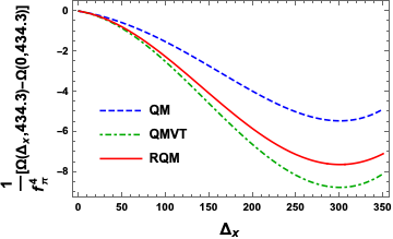
(a)  Effective potential in Nonstrange direction for $m_{\sigma}=400\ \text{MeV}$.

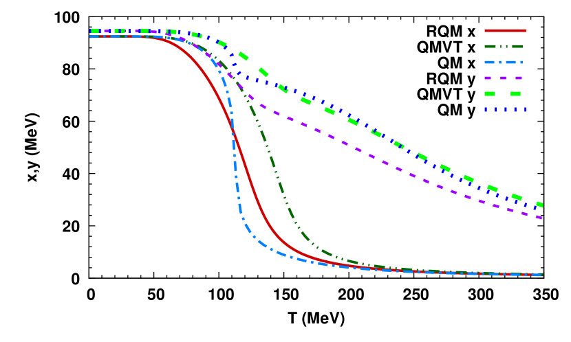
(b)  Nonstrange and strange order parameter for $m_{\sigma}=400\ \text{MeV}$.

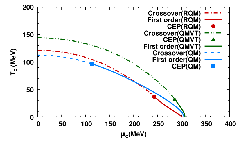
(c)  Phase diagram for $m_{\sigma}=400\ \text{MeV}$.

Figure 5:

Parameters in the different model scenarios are presented in the Table 2. The vacuum effective potential $\Omega$ is a function of the two variables $\Delta_{x}$ and $\Delta_{y}$. Its minimum is located at $\Delta_{x}=m_{u/d}=300.3$ MeV, $\Delta_{y}=m_{s}=433.34$ MeV in all the 2+1 flavor model scenarios, irrespective of the $\sigma$ meson mass values. In order to study the variation of the $\Omega$ in nonstrange direction, the $\Delta_{y}$ is fixed at 433.34 MeV and the normalized vacuum effective potential difference $\boldmath{\frac{\{\Omega_{vac}(\Delta_{x},334.43)-\Omega_{vac}(0,334.43)\}}{f_{\pi}^{4}}}$ is plotted in Fig.(5(a)) with respect to the scale independent nonstrange quark mass parameter $\Delta_{x}$ for the $m_{\sigma}=$ 400 MeV. It is most shallow for the no-sea approximation of the QM model and deepest for the QMVT model while the on-shell parameter fixing of the RQM model when compared to the QMVT model, gives a shallower effective potential. The nonstrange and strange condensate temperature variations for the $\mu=0$, are presented in Fig.(5(b)). Similar to the two flavor case RaiTiw , the sharpest QM model temperature variation of the nonstrange quark condensate $x$ becomes quite smooth for the on-shell parameterization of the RQM model and the most smooth variation of the nonstrange condensate is witnessed for the QMVT model plot. The temperature derivative of the condensate in the nonstrange and strange direction when the $\mu$=0 MeV, defines the chiral crossover transition temperature (called the pseudo-critical temperature) $T_{c}^{\chi}$ for the nonstrange direction and $T_{c}^{s}$ for the strange direction. The early and sharpest crossover transition occurs at a pseudo-critical temperature of $T_{c}^{\chi}=112.5$ MeV in the QM model and a smoother chiral transition is witnessed for the RQM model at $T_{c}^{\chi}=121.1$ MeV while a most delayed and smooth chiral crossover occurs at $T_{c}^{\chi}=144.1$ MeV in the QMVT model. The melting of the strange condensate $y$ is most significant in the RQM model when it is compared with its temperature variation in the QM and QMVT models. The Fig.(5(c)) depicts the phase diagram for the $m_{\sigma}=400$ MeV. The critical end point (CEP) location $\mu=$113.3 MeV, $T=$ 96.76 MeV of the QM model shifts significantly (similar to the results reported in earlier works guptiw ; schafwag12 ; chatmoh1 ; vkkr12 ; chatmoh2 ) to a far right position in the lower corner of the $\mu-T$ plane at $\mu=$285.91 MeV, $T=$32.23 MeV for the QMVT model setting. It is worthwhile to emphasize that due to the exact on-shell parameter fixing, the CEP in the RQM model moves to a higher position when compared with the QMVT model CEP and it gets located at a higher temperature $T=$37.03 MeV and a lower chemical potential $\mu=$ 243.12 MeV.

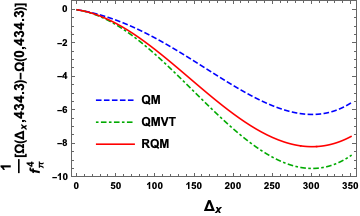
(a)  $m_{\sigma}=500\ \text{MeV}$.

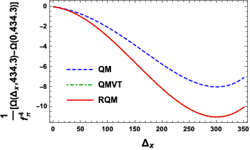
(b)  $m_{\sigma}=658.8\ \text{MeV}$.

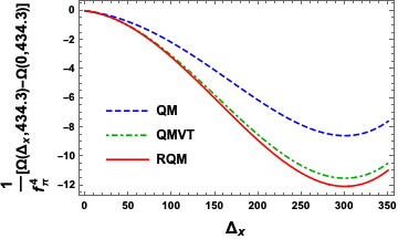
(c)  $m_{\sigma}=700\ \text{MeV}$.

Figure 6: Normalized effective potential difference in the nonstrange direction for the QM,RQM and QMVT model.

In order to see the effect of the sigma meson mass on the nature of the vacuum effective potential, the respective plots of the normalized vacuum effective potential difference $\boldmath{\frac{\{\Omega_{vac}(\Delta_{x},334.43)-\Omega_{vac}(0,334.43)\}}{f_{\pi}^{4}}}$ with respect to the nonstrange quark mass parameter $\Delta_{x}$ for the $m_{\sigma}=$ 500 MeV, 658.8 MeV and 700 MeV, have been presented in the Figs. (6(a)), (6(b)) and (6(c)). The effective potential difference is highest (i.e. it is most shallow) in the case of the QM model for every $m_{\sigma}$. Similar to the $m_{\sigma}=$ 400 MeV case, the effective potential is deepest for the QMVT model when the $m_{\sigma}=$ 500 MeV in the Fig. (6(a)) while the on-shell parameterization in the RQM model gives a shallower effective potential in comparison. When the $m_{\sigma}$ value is increased, one notices that the effective potential difference in the RQM model becomes deeper and the QMVT model effective potential difference shows a rising trend and both the effective potential plots merge with each other for the $m_{\sigma}=658.8\ \text{MeV}$, in the Fig. (6(b)). As the $m_{\sigma}$ is increased beyond the 658.8 MeV, the plot of the effective potential difference turns deepest in the RQM model.The trend seen in the Fig (6(a)) gets reversed in the plots of the Fig. (6(c)) for the $m_{\sigma}=700\text{MeV}$ case as the effective potential difference becomes shallower for the QMVT model and deepest for the RQM model. In our very recent work for the two flavor case RaiTiw , we found similar trend reversal for the $m_{\sigma}>616$ MeV.

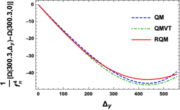
(a)   $m_{\sigma}=500\ \text{MeV}$.

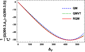
(b)   $m_{\sigma}=785\ \text{MeV}$.

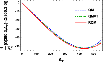
(c)  $m_{\sigma}=850\ \text{MeV}$.

Figure 7: Normalized effective potential difference in the strange direction for the QM, RQM and QMVT model.

The variation of the $\Omega$ in strange direction has also been investigated by fixing the $\Delta_{x}$ at 300.3 MeV. The normalized vacuum effective potential difference $\boldmath{\frac{\{\Omega_{vac}(300.3,\Delta_{y})-\Omega_{vac}(300.3,0)\}}{f_{\pi}^{4}}}$ is plotted with respect to the scale independent strange quark mass parameter $\Delta_{y}$ respectively in the Fig. (7(a)), (7(b)) and (7(c)) for the $m_{\sigma}=$ 500, 785 and 850 MeV. The strange direction effective potential difference is most shallow in the RQM model, deeper in the QM model and deepest in the QMVT model for the $m_{\sigma}=$ 500 MeV. It becomes deeper in the RQM model on increasing the $m_{\sigma}$ value and shows rising trend for the QMVT model. Both the effective potential plots nearly coincide with each other (similar to the nonstrange direction effective potential when the $m_{\sigma}=658.8\ \text{MeV}$) for the $m_{\sigma}=785\ \text{MeV}$ while the QM model effective potential difference looks little shallow in comparison in the Fig. (7(b)). The trend of plots in the Fig. (7(a)) gets reversed in the Fig. (7(c)) for the $m_{\sigma}=850\ \text{MeV}$ case as the strange direction effective potential difference becomes shallower for the QMVT model and deepest for the RQM model. The trend reversal in the strange direction sets in for higher sigma mass when $m_{\sigma}>785$ MeV.

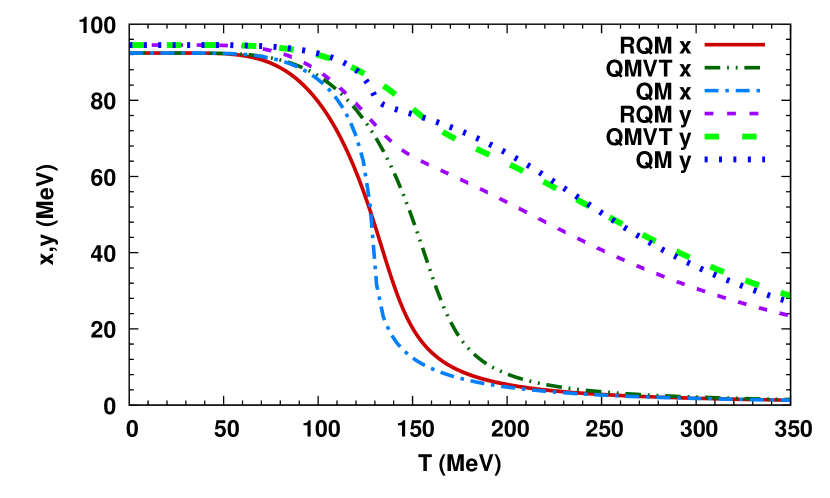
(a)   $m_{\sigma}=500\ \text{MeV}$.

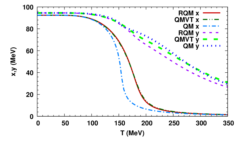
(b)   $m_{\sigma}=648\ \text{MeV}$.

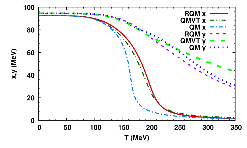
(c)   $m_{\sigma}=700\ \text{MeV}$.

Figure 8: Temperature variation of the nonstrange and strange order parameter

The temperature variations of the nonstrange and strange quark condensates $x$ and $y$ (obtained from the $\Delta_{x}$ and $\Delta_{y}$ since the renormalization does not change the Yukawa coupling $g$) at the $\mu$=0 MeV, are plotted in Fig. (8) for the three values of $m_{\sigma}=$ 500, 648 and 700 MeV. The light blue dash dotted line presents the QM model while the solid red line depicts the RQM model and the dash double dotted deep green line shows the QMVT model plot for the nonstrange quark condensate $x$. The quark one-loop vacuum correction gives rise to a smoother chiral transition in general. The sharpest nonstrange condensate temperature variation of the QM model in Fig. (8(a)) for the $m_{\sigma}=$ 500 MeV case, becomes smoother for the on-shell parameterization in the RQM model while the most smooth variation occurs in the QMVT model. The QM model nonstrange chiral crossover transition at $\mu=0$ MeV is sharpest and occurs early at a pseudo-critical temperature of $T_{c}^{\chi}=129.0$ MeV while a smoother chiral crossover for the RQM model occurs at $T_{c}=133.6$ MeV and the smoothest but delayed chiral crossover occurs in the QMVT model at $T_{c}^{\chi}=156.8$ MeV. The temperature variation of the strange quark condensate $y$ has been plotted by the thin dash line in purple for the RQM model, the dotted line in blue for the QM model and the thick dash line in green for the QMVT model.

The RQM model temperature variation of the nonstrange quark condensate almost merges with the QMVT model result when the $m_{\sigma}=$ 648 MeV in the Fig. (8(b)) and the $\mu$=0 chiral crossover transition in the nonstrange sector occurs at $T_{c}^{\chi}=178.1$ MeV in both the models. This pattern is consequence of the coincidence of the RQM model plot of the normalized vacuum effective potential difference $\boldmath{\frac{\{\Omega_{vac}(\Delta_{x},334.43)-\Omega_{vac}(0,334.43)\}}{f_{\pi}^{4}}}$ versus the $\Delta_{x}$ variation with the corresponding plot in the QMVT model in the Fig. (6(b)) for the $m_{\sigma}=$ 658.8 MeV case. Here, it is relevant to point out that in our recent work RaiTiw for the two flavor, we have shown that when the $m_{\sigma}=$ 616 MeV, the vacuum effective potential variation with respect to the constituent quark mass parameter ($\Delta$) and the chiral order parameter temperature variation for the on-shell parameter fixing scheme in the RQM model, completely merge with the corresponding effective potential and the chiral order parameter variation computed with the curvature mass parameterization in the QMVT model. In the present 2+1 flavor work, since the vacuum effective potential depends on the nonstrange and strange constituent quark mass parameter $\Delta_{x}$ and $\Delta_{y}$ variations in the two independent directions, the $\Delta_{x}$ variation of the effective potential is somewhat influenced by its $\Delta_{y}$ variation. Hence though the RQM model nonstrange direction $\Delta_{x}$ dependent variation of the vacuum effective potential difference $\boldmath{\frac{\{\Omega_{vac}(\Delta_{x},334.43)-\Omega_{vac}(0,334.43)\}}{f_{\pi}^{4}}}$ coincides with the corresponding effective potential difference variation in the QMVT model for the $m_{\sigma}=$ 658.8 MeV, the consequential coincidence of the nonstrange order parameter temperature variations for both the model settings of the RQM and QMVT, occurs when the $\sigma$ mass is smaller by about 10 MeV i.e. $m_{\sigma}=$ 648 MeV. For the $m_{\sigma}=$ 648 MeV, the temperature variation of the strange condensate $y$ in the RQM model comes closer to the corresponding results in the QM model and QMVT models. The Fig. (8(c)) when the $m_{\sigma}=$ 700 MeV, shows that the most smooth nonstrange quark condensate temperature variation takes place in the RQM model and the $\mu=0$ chiral crossover transition occurring at $T_{c}^{\chi}=195.8$ MeV, is very delayed while a less smooth chiral crossover transition is noticed in the QMVT model occurring earlier at $T_{c}^{\chi}=186.3$ MeV. Note that when the nonstrange quark condensate temperature variation in the RQM model is compared with the corresponding result in the QMVT model, one finds that the trend for the $m_{\sigma}=$ 700 MeV turns opposite of what one observes in the Fig. (8(a)) for the $m_{\sigma}=$ 500 MeV case where the RQM model condensate variation is less smooth and occurs earlier than that in the QMVT model. This happens because the nonstrange direction effective potential difference in the RQM model, becomes deepest for the $m_{\sigma}=$ 700 MeV ($>$ 658.8 MeV) case while it is shallower than that of the QMVT model for the $m_{\sigma}=$ 500 MeV ($<$658.8 MeV). The melting of the strange condensate ($y$) is most pronounced in the RQM model for the $m_{\sigma}=$ 500 MeV. Its melting in the QMVT model for the 160-240 MeV temperature range, is more than that of the QM model result. The strange condensate melting in the RQM model becomes less pronounced as the $\sigma$ meson mass is increased and its temperature variation becomes closer to the QM model result for the $m_{\sigma}=$ 648 and 700 MeV. Table 3 gives the summary of the pseudo-critical temperatures $T_{c}^{\chi}$ and $T_{c}^{s}$ for the chiral crossover transition in the nonstrange and strange direction for different $m_{\sigma}$= 400, 500, 600, 648 and 700 MeV.

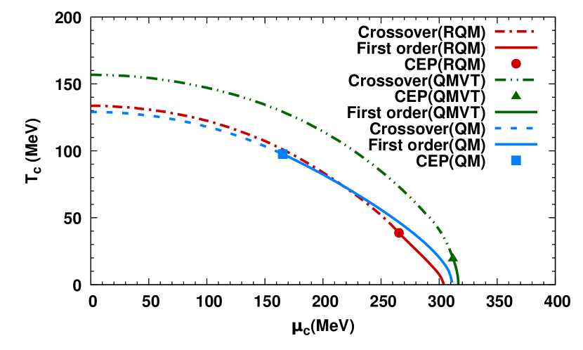
(a)   $m_{\sigma}=500$ MeV

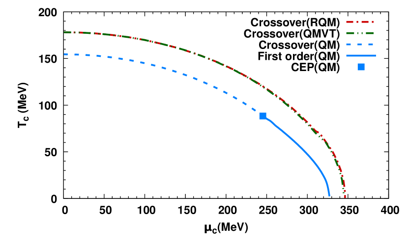
(b)   $m_{\sigma}=648$ MeV

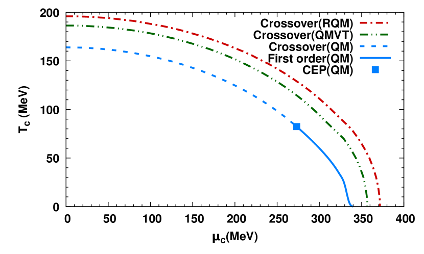
(c)   $m_{\sigma}=700$ MeV

Figure 9: Phase diagrams for different $m_{\sigma}$

The Fig. (9(a)) presents the phase diagram in the $\mu-T$ plane for the $m_{\sigma}=500$ MeV and line types for different models are labelled. The QM model critical end point (CEP) at $\mu=$165.24 MeV, $T=$97.52 MeV, shifts to a far right lower corner of the phase diagram at $\mu=$ 311.85 MeV, $T=$19.8 MeV due to the curvature mass parameterization in the QMVT model. This robust shift in the present 2+1 flavor QMVT model is larger ($\mu=$ is larger by 11 MeV and $T$ is smaller by about 10 MeV) than the corresponding shift reported RaiTiw for the two flavor QMVT model setting. It is important to note that this significantly large shift of the CEP as also reported in several of the earlier studies guptiw ; schafwag12 ; chatmoh1 ; vkkr12 ; chatmoh2 , becomes small due to the exact on-shell parameter fixing in the RQM model. The CEP in the RQM model moves relatively higher up in the phase diagram and gets located at a lower chemical potential $\mu=$265.42 MeV and higher temperature $T=$ 38.71 MeV when compared to the CEP location in the QMVT model. It is also noteworthy that the QM model and RQM model phase diagrams stand in close proximity of each other.

Similar to the two flavor RaiTiw result, here in the 2+1 flavor investigation also, the RQM model and QMVT model phase diagrams (crossover lines in the entire $\mu-T$ plane) merge with each other in the Fig. (9(b)) for the $m_{\sigma}$=648 MeV. The above overlap is consequence of the coincidence that occurs in the normalized vacuum effective potential difference and nonstrange order parameter plots respectively in the Fig. (6(b)) and Fig. (8(b))for both the models RQM and QMVT. The critical end point for the QM model gets located at $\mu=$ 223.3 MeV, $T=$ 88.37 MeV in the Fig. (9(b)). The phase diagrams for the RQM as well as the QMVT model, are crossover lines in the entire $\mu-T$ plane for the $m_{\sigma}=700$ MeV. One notices that when the $m_{\sigma}=700$ MeV in the Fig. (9(c)), instead of the RQM model phase diagram proximity to the QM model phase boundary for the $m_{\sigma}=500$ MeV, the phase diagram of the QMVT model stands closer to the QM model phase boundary. The abovementioned nature of the plots correspond to the trend reversal seen respectively in the Fig. (8(c)) and the Fig. (6(c)) for the nonstrange direction order parameter and the normalized vacuum effective potential difference when the $m_{\sigma}=700$ MeV plots are compared with the corresponding $m_{\sigma}=500$ MeV plots. In the QM model phase diagram, the first order line gets terminated at the critical end point (CEP) $\mu=$ 273.12 MeV, $T=$ 82.30 MeV.

Figure 10: Phase diagram for the sigma masses of 400, 500, 600, 648 and 700 MeV in the RQM model.

The comparison of the five phase diagrams for the $m_{\sigma}=$ 400 MeV, 500 MeV, 600 MeV, 648 MeV and 700 MeV in the RQM model and the influence of the sigma meson mass on phase diagrams can be seen in the Fig. (10). The CEP position $\mu=$ 243.12 MeV, $T=$ 37.03 MeV for the $m_{\sigma}=$ 400 MeV, shifts rightwards to $\mu=$ 265.42 MeV, $T=$ 38.71 MeV when the $m_{\sigma}=$ 500 MeV. The CEP moves to the bottom right extreme of the phase diagram at $\mu$= 317.45 MeV $T=$ 17.7 MeV for the $m_{\sigma}=$ 600 MeV. The two crossover transition lines in the whole of the $\mu-T$ plane for the $m_{\sigma}=$ 648 MeV and 700 MeV are also shown.

6 Summary and Conclusion

This work presents the first application of the on-shell parameter fixing scheme to calculate the effective potential after including the quark one-loop vacuum fluctuation and properly renormalizing it in the 2+1 flavor renormalized quark-meson (RQM) model. The seven running parameters of the model $\lambda_{1}$, $\lambda_{2}$, $c$, $m^{2}$, $h_{x}$, $h_{y}$ and $g$ are determined by relating the $\overline{\text{MS}}$, on-shell schemes and the experimental values of the pion decay constant $f_{\pi}$, the kaon decay constant $f_{K}$, the scalar $\sigma$ meson mass $m_{\sigma}$, the pseudo-scalar pion, kaon, eta and eta-prime meson masses $m_{\pi},m_{K},m_{\eta},m_{\eta^{\prime}}$ and the nonstrange as well as the strange constituent quark masses. For comparison, the earlier calculation of the effective potential in the quark-meson model with the vacuum term (QMVT) has also been presented where the curvature meson masses have been used for fixing the model parameters. We have computed and compared the effective potentials, the nonstrange and strange order parameter temperature variations and the phase diagrams for the QM, RQM and QMVT model settings.

The $\sigma$ meson mass dependent similarities and differences are observed in the plots of the vacuum effective potentials in the nonstrange and strange directions for the RQM model and the QMVT model. The nonstrange direction normalized vacuum effective potential difference, is deepest for the QMVT model when the $m_{\sigma}=$ 400 and 500 MeV while it is shallower in the RQM model and most shallow in the QM model. For the $m_{\sigma}=$658.8 MeV, the nonstrange direction vacuum effective potential difference in both the plots for the RQM and QMVT models coincide with each other and for the higher $m_{\sigma}=$ 700 ($>$ 658.8) MeV, one finds that the trend of the plots for the $m_{\sigma}=$500 MeV gets reversed and the effective potential is deepest in the RQM model. The strange direction vacuum effective potential difference is most shallow in the RQM model, deeper in the QM model and deepest in the QMVT model for the $m_{\sigma}=$ 500 MeV. It becomes deeper in the RQM model on increasing the $m_{\sigma}$ value and shows rising trend for the QMVT model. Both the effective potential plots nearly merge with each other for the $m_{\sigma}=785\ \text{MeV}$. The trend of plots for the $m_{\sigma}=500$ MeV gets reversed for the $m_{\sigma}=850$ MeV as the strange direction effective potential difference becomes shallower for the QMVT model and deepest for the RQM model.

Comparing the $\mu=0$ MeV nonstrange order parameter ($x$), one finds that its sharpest QM model temperature variation for the $m_{\sigma}=$500 MeV, becomes smoother for the on-shell parameterization of the RQM model while the curvature mass parameterization of the QMVT model gives rise to a most smooth and delayed variation. This pattern also gets reversed for the higher $m_{\sigma}=$700 ($>$648) MeV as the nonstrange order parameter temperature variation becomes most smooth and delayed for the RQM model. We point out that our recent two flavor work RaiTiw reported that, for the $m_{\sigma}=$ 616 MeV, the vacuum effective potential variation (dependent on the constituent quark mass parameter $\Delta$) and the chiral order parameter temperature variation for the on-shell parameter fixing scheme in the RQM model, completely merge with the corresponding effective potential and the chiral order parameter temperature variation computed with the curvature mass parameterization in the QMVT model. In the present 2+1 flavor work, since the vacuum effective potential depends on the nonstrange and strange constituent quark mass parameter $\Delta_{x}$ and $\Delta_{y}$ variations in the two independent directions, the $\Delta_{x}$ variation of the effective potential is somewhat influenced by its $\Delta_{y}$ variation. Hence though the RQM model nonstrange direction $\Delta_{x}$ dependent variation of the vacuum effective potential difference $\boldmath{\frac{\{\Omega_{vac}(\Delta_{x},334.43)-\Omega_{vac}(0,334.43)\}}{f_{\pi}^{4}}}$ coincides with the corresponding effective potential difference variation in the QMVT model for the $m_{\sigma}=$ 658.8 MeV, the consequential coincidence of the nonstrange order parameter temperature variations for both the model settings of the RQM and QMVT, occurs when the $\sigma$ mass is smaller by about 10 MeV i.e. $m_{\sigma}=$ 648 MeV. The melting of the strange condensate ($y$) is most pronounced in the RQM model for the $m_{\sigma}=$ 400 and 500 MeV and its melting in the QMVT model is more than that of the QM model result in the temperature range of 160-240 MeV.The strange condensate melting in the RQM model becomes less pronounced as the $\sigma$ meson mass is increased and its temperature variation comes closer to the QM model result as the value of the $m_{\sigma}$ changes from 500 MeV to 648 and 700 MeV.

It is well known that the CEP shifts to the far right side of the phase diagram in the $\mu-T$ plane for the QMVT model guptiw ; schafwag12 ; chatmoh1 ; vkkr12 ; chatmoh2 ; RaiTiw . Similar to the two flavor results RaiTiw , here in the present 2+1 flavor work also, it is noticed that when the $m_{\sigma}=$ 400, 500 ($<$ 648) MeV, the shift in the position of the CEP due to the on-shell parameterization in the RQM model, is smaller than what is found in the QMVT model. Furthermore, the phase boundaries depicting the crossover transition lines, for both the models RQM and QMVT, completely merge with each other for the $m_{\sigma}=$ 648 MeV. The crossover transition line of the QMVT model phase diagram, comes closer to the QM model phase boundary for the higher $m_{\sigma}=$ 700 ($>$ 648) MeV. This trend is opposite of what one notices for the $m_{\sigma}=$ 500 ($<$ 648) MeV case where the RQM model phase diagram stands in close proximity to the QM model phase boundary.

Appendix A THE QMVT PARAMETER FIXING

This appendix presents a brief description of the parameter fixing procedure in the QMVT model as given in Ref. vkkt13 . The vacuum meson mass matrix is written as

$$m_{\alpha,ab}^{2} = \frac{\partial^{2}\Omega^{\Lambda}(x,y)}{\partial\xi_{\alpha,a}\partial\xi_{\alpha,b}}\bigg{|}_{min}=({m^{\text{m}}_{\alpha,ab}})^{2}+({\delta m^{\text{v}}_{\alpha,ab}})^{2}\quad$$ (172)

Here, the $({m^{\text{m}}_{\alpha,ab}})^{2}$ expressions for $\alpha=\text{s, p}$ and $a,b=0,1,\cdots,8$ are same as the vacuum values of the meson masses $m_{\alpha,ab}^{2}$ which were originally evaluated for the QM model under s-MFA in Ref. Rischke:00 ; Rischke:001 ; Schaefer:09 by taking the second derivatives of the pure mesonic potential at its minimum. The vacuum ($T=0$, $\mu=0$) mass modifications on account of the fermionic vacuum correction are given by

$$({\delta m^{\text{v}}_{\alpha,ab}})^{2}=\frac{\partial^{2}\Omega_{q\bar{q}}^{\rm vac}}{\partial\xi_{\alpha,a}\partial\xi_{\alpha,b}}\bigg{|}_{min}=-\frac{N_{c}}{8\pi^{2}}\sum_{f}\biggl{[}\left(2\log\left(\frac{m_{f}}{\text{M}}\right)+\frac{3}{2}\right)\left(\frac{\partial m_{f}^{2}}{\partial\xi_{\alpha,a}}\right)\left(\frac{\partial m_{f}^{2}}{\partial\xi_{\alpha,b}}\right)$$

$${\hskip 142.26378pt}+\left(\frac{m_{f}^{2}}{2}+2m_{f}^{2}\log\left(\frac{m_{f}}{\text{M}}\right)\right)\frac{\partial^{2}m_{f}^{2}}{\partial\xi_{\alpha,a}\partial\xi_{\alpha,b}}\biggr{]}$$ (173)

Here $|_{min}$ denotes the global minimum of the full grand potential in the Eq.(13). The first $m^{2}_{f,a}\equiv\partial m^{2}_{f}/\partial\xi_{\alpha,a}$ and second $m^{2}_{f,ab}\equiv\partial m^{2}_{f,a}/\partial\xi_{\alpha,b}$ partial derivatives of the squared quark mass with respect to the different meson fields are evaluated in Ref. Schaefer:09 in the non strange-strange basis. The values of these derivatives can be found from the Table III of the Ref. Schaefer:09 ; vkkt13 . The mass modifications given in the Eq. (173) due to the fermionic vacuum correction were evaluated in the Ref. vkkt13 and different expressions of $({\delta m^{\text{v}}_{\alpha,ab}})^{2}$ are presented in the Table 4 for all the mesons of the scalar and pseudo-scalar nonet.

In the QMVT model calculations, the vacuum mass expressions in the Eq.(172) that determine $\lambda_{2}$ and c are $m^{2}_{\pi}=({m^{\text{m}}_{\pi}})^{2}+({\delta m^{\text{v}}_{\text{p},11}})^{2}$, $m^{2}_{K}=({m^{\text{m}}_{K}})^{2}+({\delta m^{\text{v}}_{p,44}})^{2}$ and $m^{2}_{\eta}+m^{2}_{\eta^{\prime}}=m^{2}_{\text{p},00}+m^{2}_{\text{p},88}$ where $m^{2}_{\text{p},00}=({m^{\text{m}}_{\text{p},00}})^{2}+({\delta m^{\text{v}}_{\text{p},00}})^{2}$ and $m^{2}_{\text{p},88}=({m^{\text{m}}_{\text{p},88}})^{2}+({\delta m^{\text{v}}_{\text{p},88}})^{2}$. We can write $m^{2}_{\eta}+m^{2}_{\eta^{\prime}}=({m^{\text{m}}_{\eta}})^{2}+({m^{\text{m}}_{\eta^{\prime}}})^{2}+({\delta m^{\text{v}}_{\text{p},00}})^{2}+({\delta m^{\text{v}}_{\text{p},88}})^{2}$ where $({m^{\text{m}}_{\eta}})^{2}+({m^{\text{m}}_{\eta^{\prime}}})^{2}=({m^{\text{m}}_{\text{p},00}})^{2}+({m^{\text{m}}_{\text{p},88}})^{2}$. Using mass modification expressions $({\delta m^{\text{v}}_{\alpha,ab}})^{2}$ given in the Table 4, one writes

$$({m^{\text{m}}_{K}})^{2} = m^{2}_{K}+\frac{N_{c}g^{4}}{64\pi^{2}}\left(\frac{x-\sqrt{2}y}{x^{2}-2y^{2}}\right)\left(x^{3}X+2\sqrt{2}y^{3}Y\right);\ ({m^{\text{m}}_{\pi}})^{2}=m^{2}_{\pi}+\frac{N_{c}g^{4}}{64\pi^{2}}\ x^{2}X\ \ \$$

$$\text{and}\left({m^{\text{m}}_{\eta}})^{2}+({m^{\text{m}}_{\eta^{\prime}}})^{2}\right)=\left(m^{2}_{\eta}+m^{2}_{\eta^{\prime}}\right)+\frac{N_{c}g^{4}}{192\pi^{2}}\left(3x^{2}X+6y^{2}Y\right)\;.$$

Table 4: The superscript m in the $({m^{\text{m}}_{\alpha,ab}})^{2}$ symbolizes the meson curvature masses calculated from the second derivatives of the pure mesonic potential U($x,y$). The mass modifications $({\delta m^{\text{v}}_{\alpha,ab}})^{2}$ due to the fermionic vacuum correction are shown in the right half. Symbols used in the expressions are defined as $X=\left\{1+4\log\left(\frac{g\ x}{2\Lambda}\right)\right\}$ and $Y=\left\{1+4\log\left(\frac{g\ y}{\sqrt{2}\Lambda}\right)\right\}$.

	Meson masses calculated from pure mesonic potential		Fermionic vacuum correction in meson masses
$(m^{\text{m}}_{a_{0}})^{2}$	$m^{2}+\lambda_{1}(x^{2}+y^{2})+\frac{3\lambda_{2}}{2}x^{2}+\frac{\sqrt{2}c}{2}y$	$({\delta m^{\text{v}}_{\text{s},11}})^{2}$	$-\frac{N_{c}g^{4}}{64\pi^{2}}\ \ x^{2}(4+3X)$
$(m^{\text{m}}_{\kappa})^{2}$	$m^{2}+\lambda_{1}(x^{2}+y^{2})+\frac{\lambda_{2}}{2}(x^{2}+\sqrt{2}xy+2y^{2})+\frac{c}{2}x$	$({\delta m^{\text{v}}_{\text{s},44}})^{2}$	$-\frac{N_{c}g^{4}}{64\pi^{2}}\ \ \left(\frac{x+\sqrt{2}y}{x^{2}-2y^{2}}\right)\left(x^{3}X-2\sqrt{2}y^{3}Y\right)$
$(m^{\text{m}}_{\text{s},00})^{2}$	$m^{2}+\frac{\lambda_{1}}{3}(7x^{2}+4\sqrt{2}xy+5y^{2})+\lambda_{2}(x^{2}+y^{2})-\frac{\sqrt{2}c}{3}(\sqrt{2}x+y)$	$({\delta m^{\text{v}}_{\text{s},00}})^{2}$	$-\frac{N_{c}g^{4}}{96\pi^{2}}\ \ \left\{3\left(x^{2}X+y^{2}Y\right)+4\left(x^{2}+y^{2}\right)\right\}$
$(m^{\text{m}}_{\text{s},88})^{2}$	$m^{2}+\frac{\lambda_{1}}{3}(5x^{2}-4\sqrt{2}xy+7y^{2})+\lambda_{2}(\frac{x^{2}}{2}+2y^{2})+\frac{\sqrt{2}c}{3}(\sqrt{2}x-\frac{y}{2})$	$({\delta m^{\text{v}}_{\text{s},88}})^{2}$	$-\frac{N_{c}g^{4}}{96\pi^{2}}\ \ \left\{\frac{3}{2}\left(x^{2}X+4y^{2}Y\right)+2\left(x^{2}+4y^{2}\right)\right\}$
$(m^{\text{m}}_{\text{s},08})^{2}$	$\frac{2\lambda_{1}}{3}(\sqrt{2}x^{2}-xy-\sqrt{2}y^{2})+\sqrt{2}\lambda_{2}(\frac{x^{2}}{2}-y^{2})+\frac{c}{3\sqrt{2}}(x-\sqrt{2}y)$	$({\delta m^{\text{v}}_{\text{s},08}})^{2}$	$-\frac{N_{c}g^{4}}{8\sqrt{2}\pi^{2}}\ \ \left\{\frac{1}{4}\left(x^{2}X-2y^{2}Y\right)+\frac{1}{3}\left(x^{2}-2y^{2}\right)\right\}$
$(m^{\text{m}}_{\pi})^{2}$	$m^{2}+\lambda_{1}(x^{2}+y^{2})+\frac{\lambda_{2}}{2}x^{2}-\frac{\sqrt{2}c}{2}y$	$({\delta m^{\text{v}}_{\text{p},11}})^{2}$	$-\frac{N_{c}g^{4}}{64\pi^{2}}\ \ x^{2}X$
$(m^{\text{m}}_{K})^{2}$	$m^{2}+\lambda_{1}(x^{2}+y^{2})+\frac{\lambda_{2}}{2}(x^{2}-\sqrt{2}xy+2y^{2})-\frac{c}{2}x$	$({\delta m^{\text{v}}_{\text{p},44}})^{2}$	$-\frac{N_{c}g^{4}}{64\pi^{2}}\ \ \left(\frac{x-\sqrt{2}y}{x^{2}-2y^{2}}\right)\left(x^{3}X+2\sqrt{2}y^{3}Y\right)$
$(m^{\text{m}}_{\text{p},00})^{2}$	$m^{2}+\lambda_{1}(x^{2}+y^{2})+\frac{\lambda_{2}}{3}(x^{2}+y^{2})+\frac{c}{3}(2x+\sqrt{2}y)$	$({\delta m^{\text{v}}_{\text{p},00}})^{2}$	$-\frac{N_{c}g^{4}}{96\pi^{2}}\ \ \left(x^{2}X+y^{2}Y\right)$
$(m^{\text{m}}_{\text{p},88})^{2}$	$m^{2}+\lambda_{1}(x^{2}+y^{2})+\frac{\lambda_{2}}{6}(x^{2}+4y^{2})-\frac{c}{6}(4x-\sqrt{2}y)$	$({\delta m^{\text{v}}_{\text{p},88}})^{2}$	$-\frac{N_{c}g^{4}}{192\pi^{2}}\ \ \left(x^{2}X+4y^{2}Y\right)$
$(m^{\text{m}}_{\text{p},08})^{2}$	$\frac{\sqrt{2}\lambda_{2}}{6}(x^{2}-2y^{2})-\frac{c}{6}(\sqrt{2}x-2y)$	$({\delta m^{\text{v}}_{\text{p},08}})^{2}$	$-\frac{N_{c}g^{4}}{96\sqrt{2}\pi^{2}}\ \ \left(x^{2}X-2y^{2}Y\right)$

The $f_{\pi}$ and $f_{K}$ give vacuum condensates according to the partially conserved axial vector current (PCAC) relation. The $x=f_{\pi}$ and $y=\left(\frac{2f_{K}-f_{\pi}}{\sqrt{2}}\right)$ at $T=0$. The parameters $\lambda_{2}$ and $c$ in vacuum are obtained as:

$$\lambda_{2} = \frac{3\left(2f_{K}-f_{\pi}\right)({m^{\text{m}}_{K}})^{2}-\left(2f_{K}+f_{\pi}\right)({m^{\text{m}}_{\pi}})^{2}-2\left(({m^{\text{m}}_{\eta}})^{2}+({m^{\text{m}}_{\eta^{\prime}}})^{2}\right)\left(f_{K}-f_{\pi}\right)}{\left(3f^{2}_{\pi}+8f_{K}\left(f_{K}-f_{\pi}\right)\right)\left(f_{K}-f_{\pi}\right)}\;,$$ (175)

$$c = \frac{({m^{\text{m}}_{K}})^{2}-({m^{\text{m}}_{\pi}})^{2}}{f_{K}-f_{\pi}}-\lambda_{2}\left(2f_{K}-f_{\pi}\right)\;.$$ (176)

When expressions of $({m^{\text{m}}_{\pi}})^{2}$, $({m^{\text{m}}_{K}})^{2}$ and $\left(({m^{\text{m}}_{\eta}})^{2}+({m^{\text{m}}_{\eta^{\prime}}})^{2}\right)$ from the Eq.(A) are substituted in the Eq.(175), the Eq.(176) and the vacuum value of the condensates are used, the final rearrangement of terms yields:

$$\lambda_{2} = \lambda_{2s}+n+\lambda_{2+}+\lambda_{2\Lambda}\ \text{where}\ \lambda_{2s}=\frac{3\left(2f_{K}-f_{\pi}\right)m^{2}_{K}-\left(2f_{K}+f_{\pi}\right)m^{2}_{\pi}-2\left(m^{2}_{\eta}+m^{2}_{\eta^{\prime}}\right)\left(f_{K}-f_{\pi}\right)}{\left(3f^{2}_{\pi}+8f_{K}\left(f_{K}-f_{\pi}\right)\right)\left(f_{K}-f_{\pi}\right)}\ ,$$ (177)

$$n = \frac{N_{c}g^{4}}{32\pi^{2}},\ \lambda_{2+}=\frac{n{f_{\pi}}^{2}}{f_{K}\left(f_{K}-f_{\pi}\right)}\log\left(\frac{2\ f_{K}-f_{\pi}}{f_{\pi}}\right)\text{and scale dependent part}\ \lambda_{2\Lambda}=4n\log\left(\frac{g\left(2f_{K}-f_{\pi}\right)}{2\Lambda}\right),$$

$$c = \frac{{m_{K}}^{2}-{m_{\pi}}^{2}}{f_{K}-f_{\pi}}-\lambda_{2s}\left(2f_{K}-f_{\pi}\right).$$ (178)

Note that the $\lambda_{2s}$ is the old $\lambda_{2}$ parameter fixed in the QM/PQM model calculations in Ref. Rischke:00 ; Rischke:001 ; Schaefer:09 ; TiPQM3F . Here, the curvature mass parameterization in the QMVT model, generates an addition of ($n+\lambda_{2+}$) to $\lambda_{2s}$ and further, one gets a scale $\Lambda$ dependent addition $\lambda_{2\Lambda}$ to the expression of the $\lambda_{2}$ in the Eq. (177). The $\Lambda$ dependence completely cancels in the evaluation of $c$ and its value remains the same as in the QM model. The parameter $m^{2}$ can be expressed in terms of $\lambda_{1}$ using the scale $\Lambda$ independent formula of $m^{2}_{\pi}$ (given in the appendix B of the Ref. vkkt13 ) and putting $x=f_{\pi}$ and $y=(\frac{2f_{K}-f_{\pi}}{\sqrt{2}})$, one gets,

$$m^{2} = m^{2}_{\pi}-\lambda_{1}\{f_{\pi}^{2}+\frac{(2f_{K}-f_{\pi})^{2}}{2}\}-\frac{f_{\pi}^{2}}{2}\ \biggl{[}\ \lambda_{2\text{v}}\qquad$$ (179)

$$-4\log\ \{\ \frac{f_{\pi}}{\left(2f_{K}-f_{\pi}\right)}\}\biggl{]}+\frac{c}{2}\ (\ 2f_{K}-f_{\pi})\;.$$

When the formula of $m^{2}_{\sigma}$ (given in the Table 1) is used with the vacuum values of the masses $m^{2}_{\text{s},00}$, $m^{2}_{\text{s},88}$, $m^{2}_{\text{s},08}$ and the above expression of $m^{2}$ is substituted in it, one gets the numerical value of $\lambda_{1}$ for different values of $m_{\sigma}$. The fermionic vacuum correction does not change the explicit symmetry breaking parameters $h_{x}$ and $h_{y}$.

Appendix B THE TADPOLE TERMS

The expressions of tadpole contributions in the self-energies are,

$$\Sigma^{tad}_{\text{s},00}=4\sqrt{\frac{2}{3}}N_{c}g\left[\frac{1}{m^{2}_{s,00}}\left\{3\left(\lambda_{1}+\frac{\lambda_{2}}{3}\right)\bar{\sigma_{0}}-\frac{c}{2}\sqrt{\frac{2}{3}}\right\}+\frac{1}{3m^{2}_{s,08}}(\lambda_{1}+\lambda_{2})\bar{(}\sigma_{8})\right]\mathcal{F}(m_{u},m_{s})$$

$$+\frac{8}{\sqrt{3}}N_{c}g\left[\frac{1}{m^{2}_{s,08}}\left\{3\left(\lambda_{1}+\frac{\lambda_{2}}{3}\right)\bar{\sigma_{0}}-\frac{c}{2}\sqrt{\frac{2}{3}}\right\}+\frac{1}{3m^{2}_{s,88}}(\lambda_{1}+\lambda_{2})\bar{\sigma_{8}}\right]\mathcal{G}(m_{u},m_{s})$$ (180)

$$\Sigma^{tad}_{\text{s},88}=4\sqrt{\frac{2}{3}}N_{c}g\left[\frac{1}{3\ m^{2}_{s,00}}\left\{\left(\lambda_{1}+\lambda_{2}\right)\bar{\sigma_{0}}-\frac{\lambda_{2}}{\sqrt{2}}\bar{\sigma_{8}}+\frac{c}{4}\sqrt{\frac{2}{3}}\right\}+\frac{1}{m^{2}_{s,08}}\left\{\frac{-\lambda_{2}}{\sqrt{2}}\bar{\sigma_{0}}+3\left(\lambda_{1}+\frac{\lambda_{2}}{2}\right)\bar{\sigma_{8}}+\frac{c}{2\sqrt{3}}\right\}\right]$$

$${\hskip-14.22636pt}\mathcal{F}(m_{u},m_{s})+\frac{8}{\sqrt{3}}N_{c}g\left[\frac{1}{3\ m^{2}_{s,08}}\left\{\left(\lambda_{1}+\lambda_{2}\right)\bar{\sigma_{0}}-\frac{\lambda_{2}}{\sqrt{2}}\bar{\sigma_{8}}+\frac{c}{4}\sqrt{\frac{2}{3}}\right\}+\frac{1}{m^{2}_{s,88}}\left\{\frac{-\lambda_{2}}{\sqrt{2}}\bar{\sigma_{0}}+3\left(\lambda_{1}+\frac{\lambda_{2}}{2}\right)\bar{\sigma_{8}}+\frac{c}{2\sqrt{3}}\right\}\right]$$

$$\mathcal{G}(m_{u},m_{s}),$$ (181)

$$\Sigma^{tad}_{\text{s},08}=4\sqrt{\frac{2}{3}}N_{c}g\left[\frac{1}{3\ m^{2}_{s,00}}(\lambda_{1}+\lambda_{2})\bar{\sigma_{8}}+\frac{1}{3\ m^{2}_{s,08}}\left\{(\lambda_{1}+\lambda_{2})\bar{\sigma_{0}}-\frac{\lambda_{2}}{\sqrt{2}}\bar{\sigma_{8}}+\frac{c}{4}\sqrt{\frac{2}{3}}\right\}\right]\mathcal{F}(m_{u},m_{s})$$

$$\qquad\quad+\frac{8}{\sqrt{3}}N_{c}g\left[\frac{1}{3\ m^{2}_{s,08}}(\lambda_{1}+\lambda_{2})\bar{\sigma_{8}}+\frac{1}{3\ m^{2}_{s,88}}\left\{(\lambda_{1}+\lambda_{2})\bar{\sigma_{0}}-\frac{\lambda_{2}}{\sqrt{2}}\bar{\sigma_{8}}+\frac{c}{4}\sqrt{\frac{2}{3}}\right\}\right]\mathcal{G}(m_{u},m_{s})\;, \Sigma^{tad}_{\text{p},00}=4\sqrt{\frac{2}{3}}N_{c}g\left[\frac{1}{m^{2}_{s,00}}\left\{\left(\lambda_{1}+\frac{\lambda_{2}}{3}\right)\bar{\sigma_{0}}+\frac{c}{2}\sqrt{\frac{2}{3}}\right\}+\frac{1}{m^{2}_{s,08}}\left(\lambda_{1}+\frac{\lambda_{2}}{3}\right)\bar{\sigma_{8}}\right]\mathcal{F}(m_{u},m_{s})$$

$$\qquad\quad+\frac{8}{\sqrt{3}}N_{c}g\left[\frac{1}{m^{2}_{s,08}}\left\{\left(\lambda_{1}+\frac{\lambda_{2}}{3}\right)\bar{\sigma_{0}}+\frac{c}{2}\sqrt{\frac{2}{3}}\right\}+\frac{1}{m^{2}_{s,88}}\left(\lambda_{1}+\frac{\lambda_{2}}{3}\right)\bar{\sigma_{8}}\right]\mathcal{G}(m_{u},m_{s})\;,$$ (182)

$$\Sigma^{tad}_{\text{p},88}=4\sqrt{\frac{2}{3}}N_{c}g\left[\frac{1}{m^{2}_{s,00}}\left\{\left(\lambda_{1}+\frac{\lambda_{2}}{3}\right)\bar{\sigma_{0}}-\frac{\lambda_{2}}{3\sqrt{2}}\bar{\sigma_{8}}-\frac{c}{4}\sqrt{\frac{2}{3}}\right\}+\frac{1}{m^{2}_{s,08}}\left\{\left(\lambda_{1}+\frac{\lambda_{2}}{2}\right)\bar{\sigma_{8}}-\frac{\lambda_{2}}{3\sqrt{2}}\bar{\sigma_{0}}-\frac{c}{2\sqrt{3}}\right\}\right]$$

$${\hskip-11.38092pt}\mathcal{F}(m_{u},m_{s})+\frac{8}{\sqrt{3}}N_{c}g\left[\frac{1}{m^{2}_{s,08}}\left\{\left(\lambda_{1}+\frac{\lambda_{2}}{3}\right)\bar{\sigma_{0}}-\frac{\lambda_{2}}{3\sqrt{2}}\bar{\sigma_{8}}-\frac{c}{4}\sqrt{\frac{2}{3}}\right\}+\frac{1}{m^{2}_{s,88}}\left\{\left(\lambda_{1}+\frac{\lambda_{2}}{2}\right)\bar{\sigma_{8}}-\frac{\lambda_{2}}{3\sqrt{2}}\bar{\sigma_{0}}-\frac{c}{2\sqrt{3}}\right\}\right],$$

$$\mathcal{G}(m_{u},m_{s})$$ (183)

$$\Sigma^{tad}_{\text{p},08}=4\sqrt{\frac{2}{3}}N_{c}g\left[\frac{1}{m^{2}_{s,00}}\left(\lambda_{1}+\frac{\lambda_{2}}{3}\right)\bar{\sigma_{8}}+\frac{1}{m^{2}_{s,08}}\left\{\left(\lambda_{1}+\frac{\lambda_{2}}{3}\right)\bar{\sigma_{0}}-\frac{\lambda_{2}}{3\sqrt{2}}\bar{\sigma_{8}}-\frac{c}{4}\sqrt{\frac{2}{3}}\right\}\right]\mathcal{F}(m_{u},m_{s})$$

$$\qquad\quad+\frac{8}{\sqrt{3}}N_{c}g\left[\frac{1}{m^{2}_{s,08}}\left(\lambda_{1}+\frac{\lambda_{2}}{3}\right)\bar{\sigma_{8}}+\frac{1}{m^{2}_{s,88}}\left\{\left(\lambda_{1}+\frac{\lambda_{2}}{3}\right)\bar{\sigma_{0}}-\frac{\lambda_{2}}{3\sqrt{2}}\bar{\sigma_{8}}-\frac{c}{4}\sqrt{\frac{2}{3}}\right\}\right]\mathcal{G}(m_{u},m_{s})\;,$$ (184)

$${\hskip-28.45274pt}\Sigma^{tad}_{\text{p},11}=4\sqrt{\frac{2}{3}}N_{c}g\left[\frac{1}{m^{2}_{s,00}}\left\{\left(\lambda_{1}+\frac{\lambda_{2}}{3}\right)\bar{\sigma_{0}}+\frac{\sqrt{2}}{6}\lambda_{2}\bar{\sigma_{8}}-\frac{c}{4}\sqrt{\frac{2}{3}}\right\}+\frac{1}{m^{2}_{s,08}}\left\{\frac{\sqrt{2}}{6}\lambda_{2}\bar{\sigma_{0}}+\left(\lambda_{1}+\frac{\lambda_{2}}{6}\right)\bar{\sigma_{8}}+\frac{c}{2\sqrt{3}}\right\}\right]$$

$${\hskip-28.45274pt}\mathcal{F}(m_{u},m_{s})+\frac{8}{\sqrt{3}}N_{c}g\left[\frac{1}{m^{2}_{s,08}}\left\{\left(\lambda_{1}+\frac{\lambda_{2}}{3}\right)\bar{\sigma_{0}}+\frac{\sqrt{2}}{6}\lambda_{2}\bar{\sigma_{8}}-\frac{c}{4}\sqrt{\frac{2}{3}}\right\}+\frac{1}{m^{2}_{s,88}}\left\{\frac{\sqrt{2}}{6}\lambda_{2}\bar{\sigma_{0}}+\left(\lambda_{1}+\frac{\lambda_{2}}{6}\right)\bar{\sigma_{8}}+\frac{c}{2\sqrt{3}}\right\}\right]$$

$$\mathcal{G}(m_{u},m_{s})$$ (185)

$${\hskip-28.45274pt}\Sigma^{tad}_{\text{p},44}=4\sqrt{\frac{2}{3}}N_{c}g\left[\frac{1}{m^{2}_{s,00}}\left\{\left(\lambda_{1}+\frac{\lambda_{2}}{3}\right)\bar{\sigma_{0}}-\frac{\lambda_{2}}{6\sqrt{2}}\bar{\sigma_{8}}-\frac{c}{4}\sqrt{\frac{2}{3}}\right\}+\frac{1}{m^{2}_{s,08}}\left\{-\frac{\lambda_{2}}{6\sqrt{2}}\bar{\sigma_{0}}+\left(\lambda_{1}+\frac{7\lambda_{2}}{6}\right)\bar{\sigma_{8}}-\frac{c}{4\sqrt{3}}\right\}\right]$$

$${\hskip-28.45274pt}\mathcal{F}(m_{u},m_{s})+\frac{8}{\sqrt{3}}N_{c}g\left[\frac{1}{m^{2}_{s,08}}\left\{\left(\lambda_{1}+\frac{\lambda_{2}}{3}\right)\bar{\sigma_{0}}-\frac{\lambda_{2}}{6\sqrt{2}}\bar{\sigma_{8}}-\frac{c}{4}\sqrt{\frac{2}{3}}\right\}+\frac{1}{m^{2}_{s,88}}\left\{-\frac{\lambda_{2}}{6\sqrt{2}}\bar{\sigma_{0}}+\left(\lambda_{1}+\frac{7\lambda_{2}}{6}\right)\bar{\sigma_{8}}-\frac{c}{4\sqrt{3}}\right\}\right]$$

$$\mathcal{G}(m_{u},m_{s})$$

where $\mathcal{F}(m_{u},m_{s})=2m_{u}\mathcal{A}(m_{u}^{2})+m_{s}\mathcal{A}(m_{s}^{2})$ and $\mathcal{G}(m_{u},m_{s})=m_{u}\mathcal{A}(m_{u}^{2})-m_{s}\mathcal{A}(m_{s}^{2})$. Substituting $\bar{\sigma_{0}}=\frac{\sqrt{2}\ x+y}{\sqrt{3}}$ and $\bar{\sigma_{8}}=\frac{x-\sqrt{2}\ y}{\sqrt{3}}$ in the Eqs. (180) to (B) and rearranging the terms, one gets the following $x$ and $y$ dependent expressions of self energies for the tadpole terms.

$$\Sigma^{tad}_{\text{s},00}=\frac{8N_{c}\ g\ m_{u}\ \mathcal{A}(m_{u}^{2})}{3}\Biggl{[}-c\biggl{(}\frac{1}{m^{2}_{s,00}}+\frac{1}{\sqrt{2}\ m^{2}_{s,88}}\biggr{)}+x\left\{\frac{2\left(3\lambda_{1}+\lambda_{2}\right)}{m^{2}_{s,00}}+\frac{\left(\lambda_{1}+\lambda_{2}\right)}{3\ m^{2}_{s,88}}+\frac{2\sqrt{2}\left(2\lambda_{1}+\lambda_{2}\right)}{3\ m^{2}_{s,08}}\right\}$$

$$\qquad\quad+y\left\{\sqrt{2}\left(\frac{1}{m^{2}_{s,00}}-\frac{1}{3\ m^{2}_{s,88}}\right)\biggl{(}3\lambda_{1}+\lambda_{2}\biggr{)}+\frac{\left(\lambda_{1}-\lambda_{2}\right)}{3\ m^{2}_{s,08}}\right\}\Biggr{]}+\frac{4N_{c}\ gm_{s}\mathcal{A}(m_{s}^{2})}{3}\Biggl{[}-c\biggl{(}\frac{1}{m^{2}_{s,00}}-\frac{\sqrt{2}}{m^{2}_{s,08}}\biggr{)}$$

$${\hskip-17.07182pt}+x\left\{\frac{2\left(3\lambda_{1}+\lambda_{2}\right)}{m^{2}_{s,00}}-\frac{2\left(\lambda_{1}+\lambda_{2}\right)}{3\ m^{2}_{s,88}}-\frac{\sqrt{2}\left(17\lambda_{1}+5\lambda_{2}\right)}{3\ m^{2}_{s,08}}\right\}+y\left\{\frac{\sqrt{2}\left(3\lambda_{1}+\lambda_{2}\right)}{m^{2}_{s,00}}-\frac{2\sqrt{2}\left(\lambda_{1}+\lambda_{2}\right)}{3\ m^{2}_{s,88}}-\frac{2\left(5\lambda_{1}+2\lambda_{2}\right)}{3\ m^{2}_{s,08}}\right\}\Biggr{]}\;,$$ (187)

$$\Sigma^{tad}_{\text{s},88}=\frac{8N_{c}gm_{u}\mathcal{A}(m_{u}^{2})}{3}\Biggl{[}c\biggl{(}\frac{1}{6m^{2}_{s,00}}+\frac{7}{6\sqrt{2}m^{2}_{s,08}}+\frac{1}{2\ m^{2}_{s,88}}\biggr{)}+x\left\{\frac{\left(2\lambda_{1}+\lambda_{2}\right)}{3\ m^{2}_{s,00}}+\frac{4\left(5\lambda_{1}+\lambda_{2}\right)}{3\sqrt{2}\ m^{2}_{s,08}}+\frac{\left(6\lambda_{1}+\lambda_{2}\right)}{2\ m^{2}_{s,88}}\right\}$$

$$\qquad\quad+y\left\{\frac{\sqrt{2}(\lambda_{1}+2\lambda_{2})}{3\ m^{2}_{s,00}}-\frac{\sqrt{2}}{m^{2}_{s,88}}(3\lambda_{1}+2\lambda_{2})-\frac{\left(17\lambda_{1}+10\lambda_{2}\right)}{3\ m^{2}_{s,08}}\right\}\Biggr{]}+\frac{4N_{c}gm_{s}\mathcal{A}(m_{s}^{2})}{3}$$

$$\Biggl{[}c\biggl{(}\frac{1}{6m^{2}_{s,00}}+\frac{\sqrt{2}}{3m^{2}_{s,08}}-\frac{1}{m^{2}_{s,88}}\biggr{)}+x\left\{\frac{(2\lambda_{1}+\lambda_{2})}{3\ m^{2}_{s,00}}+\frac{\sqrt{2}(14\lambda_{1}+\lambda_{2})}{6\ m^{2}_{s,08}}-\frac{(6\lambda_{1}+\lambda_{2})}{\ m^{2}_{s,88}}\right\}$$

$$+y\left\{\frac{\sqrt{2}(\lambda_{1}+2\lambda_{2})}{3\ m^{2}_{s,00}}-\frac{4\ (5\lambda_{1}+4\lambda_{2})}{3\ m^{2}_{s,08}}+\frac{2\sqrt{2}\left(3\lambda_{1}+2\lambda_{2}\right)}{\ m^{2}_{s,88}}\right\}\Biggr{]}$$ (188)

$$\Sigma^{tad}_{\text{s},08}=\frac{8N_{c}\ g\ m_{u}\ \mathcal{A}(m_{u}^{2})}{9}\Biggl{[}c\biggl{(}\frac{1}{2m^{2}_{s,08}}+\frac{1}{2\sqrt{2}\ m^{2}_{s,88}}\biggr{)}+x\left\{\frac{\sqrt{2}\left(\lambda_{1}+\lambda_{2}\right)}{m^{2}_{s,00}}+\frac{\left(3\lambda_{1}+2\lambda_{2}\right)}{\ m^{2}_{s,08}}+\frac{\left(2\lambda_{1}+\lambda_{2}\right)}{\sqrt{2}\ m^{2}_{s,88}}\right\}\;$$

$$\qquad\quad+y\left\{\frac{-2(\lambda_{1}+\lambda_{2})}{m^{2}_{s,00}}+\frac{\sqrt{2}\lambda_{2}}{m^{2}_{s,08}}+\frac{\left(\lambda_{1}+2\lambda_{2}\right)}{m^{2}_{s,88}}\right\}\Biggr{]}+\frac{4N_{c}\ g\ m_{s}\mathcal{A}(m_{s}^{2})}{9}\Biggl{[}c\biggl{(}\frac{1}{2\ m^{2}_{s,08}}-\frac{1}{\sqrt{2}\ m^{2}_{s,88}}\biggr{)}$$

$$+x\left\{\frac{\sqrt{2}\left(\lambda_{1}+\lambda_{2}\right)}{m^{2}_{s,00}}-\frac{\lambda_{2}}{m^{2}_{s,08}}-\frac{\sqrt{2}\left(2\lambda_{1}+\lambda_{2}\right)}{m^{2}_{s,88}}\right\}+y\left\{\frac{-2(\lambda_{1}+\lambda_{2})}{m^{2}_{s,00}}+\frac{\sqrt{2}(3\lambda_{1}+4\lambda_{2})}{m^{2}_{s,08}}-\frac{2\left(\lambda_{1}+2\lambda_{2}\right)}{m^{2}_{s,88}}\right\}\Biggr{]}\;,$$ (189)

$$\Sigma^{tad}_{\text{p},00}=\frac{8N_{c}\ g\ m_{u}\ \mathcal{A}(m_{u}^{2})}{3}\Biggl{[}c\biggl{(}\frac{1}{m^{2}_{s,00}}+\frac{1}{\sqrt{2}\ m^{2}_{s,08}}\biggr{)}+x\biggl{(}\lambda_{1}+\frac{\lambda_{2}}{3}\biggr{)}\left\{\frac{2}{m^{2}_{s,00}}+\frac{2\sqrt{2}}{m^{2}_{s,08}}+\frac{1}{m^{2}_{s,88}}\right\}$$

$$\qquad\quad+y\biggl{(}\lambda_{1}+\frac{\lambda_{2}}{3}\biggr{)}\left\{\frac{\sqrt{2}}{m^{2}_{s,00}}-\frac{1}{m^{2}_{s,08}}-\frac{\sqrt{2}}{m^{2}_{s,88}}\right\}\Biggr{]}+\frac{4N_{c}\ gm_{s}\mathcal{A}(m_{s}^{2})}{3}\Biggl{[}c\biggl{(}\frac{1}{m^{2}_{s,00}}-\frac{\sqrt{2}}{m^{2}_{s,08}}\biggr{)}$$

$$\qquad\quad+x\biggl{(}\lambda_{1}+\frac{\lambda_{2}}{3}\biggr{)}\left\{\frac{2}{m^{2}_{s,00}}-\frac{\sqrt{2}}{m^{2}_{s,08}}-\frac{2}{m^{2}_{s,88}}\right\}+y\biggl{(}\lambda_{1}+\frac{\lambda_{2}}{3}\biggr{)}\left\{\frac{\sqrt{2}}{m^{2}_{s,00}}-\frac{4}{m^{2}_{s,08}}+\frac{2\sqrt{2}}{m^{2}_{s,88}}\right\}\Biggr{]}\;,$$ (190)

$${\hskip-28.45274pt}\Sigma^{tad}_{\text{p},88}=\frac{8N_{c}gm_{u}\mathcal{A}(m_{u}^{2})}{3}\Biggl{[}-\frac{c}{2}\biggl{(}\frac{1}{m^{2}_{s,00}}+\frac{3}{\sqrt{2}m^{2}_{s,08}}+\frac{1}{\ m^{2}_{s,88}}\biggr{)}+x\left\{\frac{\left(2\lambda_{1}+\frac{\lambda_{2}}{3}\right)}{\ m^{2}_{s,00}}+\frac{\sqrt{2}\left(2\lambda_{1}+\frac{\lambda_{2}}{3}\right)}{m^{2}_{s,08}}+\frac{\left(\lambda_{1}+\frac{\lambda_{2}}{6}\right)}{m^{2}_{s,88}}\right\}$$

$$+y\left\{\frac{\sqrt{2}(\lambda_{1}+\frac{2\lambda_{2}}{3})}{\ m^{2}_{s,00}}-\frac{1}{m^{2}_{s,08}}(\lambda_{1}+\frac{2\lambda_{2}}{3})-\frac{\sqrt{2}(\lambda_{1}+\frac{\lambda_{2}}{3})}{\ m^{2}_{s,88}}\right\}\Biggr{]}+\frac{4N_{c}gm_{s}\mathcal{A}(m_{s}^{2})}{3}\Biggl{[}-c\biggl{(}\frac{1}{2m^{2}_{s,00}}-\frac{1}{m^{2}_{s,88}}\biggr{)}$$

$${\hskip-28.45274pt}+x\left\{\frac{\left(2\lambda_{1}+\frac{\lambda_{2}}{3}\right)}{\ m^{2}_{s,00}}-\frac{\sqrt{2}\left(\lambda_{1}-\frac{\lambda_{2}}{6}\right)}{m^{2}_{s,08}}-\frac{2\left(\lambda_{1}+\frac{\lambda_{2}}{6}\right)}{m^{2}_{s,88}}\right\}+y\left\{\frac{\sqrt{2}(\lambda_{1}+\frac{2\lambda_{2}}{3})}{\ m^{2}_{s,00}}-\frac{4}{m^{2}_{s,08}}(\lambda_{1}+\frac{2\lambda_{2}}{3})+\frac{2\sqrt{2}(\lambda_{1}+\frac{2\lambda_{2}}{3})}{\ m^{2}_{s,88}}\right\}\Biggr{]}\;,$$ (191)

$$\Sigma^{tad}_{\text{p},08}=\frac{8N_{c}\ g\ m_{u}\ \mathcal{A}(m_{u}^{2})}{3}\Biggl{[}-\frac{c}{2}\biggl{(}\frac{1}{\ m^{2}_{s,08}}+\frac{\sqrt{2}}{\ m^{2}_{s,88}}\biggr{)}+x\left\{\frac{\sqrt{2}\left(\lambda_{1}+\frac{\lambda_{2}}{3}\right)}{\ m^{2}_{s,00}}+\frac{\left(3\lambda_{1}+\frac{2\lambda_{2}}{3}\right)}{m^{2}_{s,08}}+\frac{\sqrt{2}\left(\lambda_{1}+\frac{\lambda_{2}}{6}\right)}{m^{2}_{s,88}}\right\}$$

$$\qquad\quad+y\left\{-2\frac{(\lambda_{1}+\frac{2\lambda_{2}}{3})}{\ m^{2}_{s,00}}+\frac{\sqrt{2}}{m^{2}_{s,08}}(\frac{\lambda_{2}}{3})+\frac{(\lambda_{1}+\frac{2\lambda_{2}}{3})}{\ m^{2}_{s,88}}\right\}\Biggr{]}+\frac{4N_{c}gm_{s}\mathcal{A}(m_{s}^{2})}{3}\Biggl{[}\frac{-c}{2}\biggl{(}\frac{1}{m^{2}_{s,08}}-\frac{\sqrt{2}}{m^{2}_{s,88}}\biggr{)}$$

$${\hskip-28.45274pt}+x\left\{\frac{\sqrt{2}\left(\lambda_{1}+\frac{\lambda_{2}}{3}\right)}{\ m^{2}_{s,00}}-\frac{\lambda_{2}}{3m^{2}_{s,08}}+\frac{-2\sqrt{2}\left(\lambda_{1}+\frac{\lambda_{2}}{6}\right)}{m^{2}_{s,88}}\right\}+y\left\{\frac{-2(\lambda_{1}+\frac{\lambda_{2}}{3})}{\ m^{2}_{s,00}}+\frac{\sqrt{2}}{m^{2}_{s,08}}(3\lambda_{1}+\frac{4\lambda_{2}}{3})-\frac{2(\lambda_{1}+\frac{2\lambda_{2}}{3})}{\ m^{2}_{s,88}}\right\}\Biggr{]}\;,$$ (192)

$$\Sigma^{tad}_{\text{p},11}=\frac{8N_{c}\ g\ m_{u}\ \mathcal{A}(m_{u}^{2})}{3}\Biggl{[}\frac{c}{2}\biggl{(}\frac{-1}{m^{2}_{s,00}}+\frac{1}{\sqrt{2}\ m^{2}_{s,08}}+\frac{1}{m^{2}_{s,88}}\biggr{)}+x\biggl{(}\lambda_{1}+\frac{\lambda_{2}}{2}\biggr{)}\left\{\frac{2}{m^{2}_{s,00}}+\frac{2\sqrt{2}}{m^{2}_{s,08}}+\frac{1}{m^{2}_{s,88}}\right\}$$

$$\qquad\quad+y\ \lambda_{1}\left\{\frac{\sqrt{2}}{m^{2}_{s,00}}-\frac{1}{m^{2}_{s,08}}-\frac{\sqrt{2}}{m^{2}_{s,88}}\right\}\Biggr{]}+\frac{4N_{c}\ gm_{s}\mathcal{A}(m_{s}^{2})}{3}\Biggl{[}\frac{c}{2}\biggl{(}\frac{-1}{m^{2}_{s,00}}+\frac{2\sqrt{2}}{m^{2}_{s,08}}-\frac{2}{m^{2}_{s,88}}\biggr{)}$$

$$\qquad\quad+x\biggl{(}\lambda_{1}+\frac{\lambda_{2}}{2}\biggr{)}\left\{\frac{2}{m^{2}_{s,00}}-\frac{\sqrt{2}}{m^{2}_{s,08}}-\frac{2}{m^{2}_{s,88}}\right\}+y\ \lambda_{1}\left\{\frac{\sqrt{2}}{m^{2}_{s,00}}-\frac{4}{m^{2}_{s,08}}+\frac{2\sqrt{2}}{m^{2}_{s,88}}\right\}\Biggr{]}\;,$$ (193)

$${\hskip-28.45274pt}\Sigma^{tad}_{\text{p},44}=\frac{8N_{c}\ g\ m_{u}\ \mathcal{A}(m_{u}^{2})}{3}\Biggl{[}-\frac{c}{4}\biggl{(}\frac{2}{\ m^{2}_{s,00}}+\frac{2\sqrt{2}}{\ m^{2}_{s,08}}+\frac{1}{\ m^{2}_{s,88}}\biggr{)}+x\left\{\frac{2\left(\lambda_{1}+\frac{\lambda_{2}}{4}\right)}{\ m^{2}_{s,00}}+\frac{\sqrt{2}\left(2\lambda_{1}+\frac{5\lambda_{2}}{4}\right)}{m^{2}_{s,08}}+\frac{\left(\lambda_{1}+\lambda_{2}\right)}{m^{2}_{s,88}}\right\}$$

$${\hskip-14.22636pt}+y\left\{\frac{\sqrt{2}(\lambda_{1}+\frac{\lambda_{2}}{2})}{\ m^{2}_{s,00}}-\frac{1}{m^{2}_{s,08}}(\lambda_{1}+2\lambda_{2})-\frac{\sqrt{2}(\lambda_{1}+\frac{5\lambda_{2}}{4})}{\ m^{2}_{s,88}}\right\}\Biggr{]}+\frac{4N_{c}gm_{s}\mathcal{A}(m_{s}^{2})}{3}\Biggl{[}-\frac{c}{4}\biggl{(}\frac{2}{\ m^{2}_{s,00}}-\frac{\sqrt{2}}{\ m^{2}_{s,08}}-\frac{2}{\ m^{2}_{s,88}}\biggr{)}$$

$${\hskip-28.45274pt}+x\left\{\frac{2\left(\lambda_{1}+\frac{\lambda_{2}}{4}\right)}{\ m^{2}_{s,00}}-\frac{\sqrt{2}\left(\lambda_{1}-\frac{\lambda_{2}}{2}\right)}{m^{2}_{s,08}}-\frac{2\left(\lambda_{1}+\lambda_{2}\right)}{m^{2}_{s,88}}\right\}+y\left\{\frac{\sqrt{2}(\lambda_{1}+\frac{\lambda_{2}}{2})}{\ m^{2}_{s,00}}-\frac{2}{m^{2}_{s,08}}(2\lambda_{1}+\frac{7\lambda_{2}}{4})+\frac{2\sqrt{2}(\lambda_{1}+\frac{5\lambda_{2}}{4})}{\ m^{2}_{s,88}}\right\}\Biggr{]}\;.$$ (194)

Appendix C INTEGRALS AND SUM INTEGRALS

The divergent loop integrals are regularized by incorporating dimensional regularization.

$$\int_{p}=\left(\frac{e^{\gamma_{E}}\Lambda^{2}}{4\pi}\right)^{\epsilon}\int\frac{d^{d}p}{(2\pi)^{d}}\;,$$ (195)

where $d=4-2\epsilon$ , $\gamma_{E}$ is the Euler-Mascheroni constant, and $\Lambda$ is renormalization scale associated with the $\overline{\text{MS}}$.

$$\mathcal{A}(m^{2}_{f}) = \int_{p}\frac{1}{p^{2}-m^{2}_{f}}=\frac{im^{2}_{f}}{(4\pi)^{2}}\left[\frac{1}{\epsilon}+1\right.$$

$$\left.+\ln(4\pi e^{-\gamma_{E}})+\ln\left(\frac{\Lambda^{2}}{m^{2}_{f}}\right)\right]\;,$$

we rewrite this after redefining $\Lambda^{2}\longrightarrow\Lambda^{2}\frac{e^{\gamma_{E}}}{4\pi}$.

$$\mathcal{A}(m^{2}_{f}) = \frac{im^{2}_{f}}{(4\pi)^{2}}\left[\frac{1}{\epsilon}+1+\ln\left(\frac{\Lambda^{2}}{m^{2}_{f}}\right)\right]\;,$$ (196)

$$\mathcal{B}(p^{2},m_{f}) = \int_{k}\frac{1}{(k^{2}-m^{2}_{f})[(k+p)^{2}-m^{2}_{f})]}$$ (197)

$$= \frac{i}{(4\pi)^{2}}\left[\frac{1}{\epsilon}+\ln\left(\frac{\Lambda^{2}}{m^{2}_{f}}\right)+\mathcal{C}(p^{2},m_{f})\right]\;,$$

$$\mathcal{B}^{\prime}(p^{2},m_{f}) = \frac{i}{(4\pi)^{2}}\mathcal{C}^{\prime}(p^{2},m_{f})\;,$$ (198)

$${\hskip-28.45274pt}\mathcal{C}(p^{2},m_{f})=2-2\sqrt{\dfrac{4m^{2}_{f}}{p^{2}}-1}\arctan\left(\dfrac{1}{\sqrt{\dfrac{4m^{2}_{f}}{p^{2}}-1}}\right);\quad\mathcal{C}^{\prime}(p^{2},m_{f})=\frac{4m^{2}_{f}}{p^{4}\sqrt{\dfrac{4m^{2}_{f}}{p^{2}}-1}}\arctan\left(\dfrac{1}{\sqrt{\dfrac{4m^{2}_{f}}{p^{2}}-1}}\right)-\frac{1}{p^{2}}\;,$$ (199)

$${\hskip-28.45274pt}\mathcal{C}(p^{2},m_{f})=2+\sqrt{1-\dfrac{4m^{2}_{f}}{p^{2}}}\ln\left(\dfrac{1-\sqrt{1-\dfrac{4m^{2}_{f}}{p^{2}}}}{1+\sqrt{1-\dfrac{4m^{2}_{f}}{p^{2}}}}\right);\quad\mathcal{C}^{\prime}(p^{2},m_{f})=\frac{2m^{2}_{f}}{p^{4}\sqrt{\dfrac{4m^{2}_{f}}{p^{2}}-1}}\ln\left(\dfrac{1-\sqrt{1-\dfrac{4m^{2}_{f}}{p^{2}}}}{1+\sqrt{1-\dfrac{4m^{2}_{f}}{p^{2}}}}\right)-\frac{1}{p^{2}}\;,$$ (200)

The Eqs.(199) and (200) are valid with the constraints ($p^{2}<4m^{2}_{f}$) and ($p^{2}>4m^{2}_{f}$) respectively.

$$\mathcal{B}(p^{2},m_{u},m_{s})=\int_{k}\frac{1}{(k^{2}-m^{2}_{s})[(k+p)^{2}-m^{2}_{u})]}=\frac{i}{(4\pi)^{2}}\left[\frac{1}{\epsilon}+\ln\left(\frac{\Lambda^{2}}{m^{2}_{u}}\right)+\mathcal{C}(p^{2},m_{u},m_{s})\right]\;,$$ (201)

$${\hskip-28.45274pt}\mathcal{C}(p^{2},m_{u},m_{s})=2-\frac{1}{2}\Biggl{[}1+\frac{m_{s}^{2}-m_{u}^{2}}{p^{2}}\Biggr{]}\ln\left(\frac{m_{s}^{2}}{m_{u}^{2}}\right)-\frac{\mathcal{G}(p^{2})}{p^{2}}\Biggl{[}\arctan\left(\frac{p^{2}-m^{2}_{s}+m^{2}_{u}}{\mathcal{G}(p^{2})}\right)+\arctan\left(\frac{p^{2}+m^{2}_{s}-m^{2}_{u}}{\mathcal{G}(p^{2})}\right)\Biggr{]}\;,\quad\quad$$ (202)

$$\mathcal{G}(p^{2})=\sqrt{\{(m_{s}+m_{u})^{2}-p^{2}\}\{p^{2}-(m_{s}-m_{u})^{2}\}}\;,$$ (203)

$$\mathcal{C}^{\prime}(p^{2},m_{u},m_{s})=\frac{m_{s}^{2}-m_{u}^{2}}{2p^{4}}\ln\Biggl{(}\frac{m^{2}_{s}}{m^{2}_{u}}\Biggr{)}+\frac{p^{2}(m_{s}^{2}+m_{u}^{2})-(m_{s}^{2}-m_{u}^{2})^{2}}{p^{4}\mathcal{G}(p^{2})}\Biggl{[}\arctan\Biggl{(}\frac{(p^{2}-m^{2}_{s}+m^{2}_{u})}{\mathcal{G}(p^{2})}\Biggr{)}$$

$$\qquad\qquad\qquad\quad+\arctan\Biggl{(}\frac{(p^{2}+m^{2}_{s}-m^{2}_{u})}{\mathcal{G}(p^{2})}\Biggr{)}\Biggr{]}-\frac{1}{p^{2}}\;.$$ (204)

References

• (1) N. Cabibbo and G. Parisi, Exponential Hadronic Spectrum and Quark Liberation, Phys. Lett. B 59, (1975) 67-69.
• (2) L. D. McLerran and B. Svetitsky, Quark Liberation at High Temperature: A Monte Carlo Study of SU(2) Gauge Theory, Phys. Rev. D 24,(1981) 450.
• (3) B. Svetitsky, Symmetry Aspects of Finite Temperature Confinement Transitions, Phys. Rep. 132, (1986) 1.
• (4) B. Muller, Physics and signatures of the quark - gluon plasma, Rep. Prog. Phys. 58, (1995) 611.
• (5) H. Meyer-Ortmanns, Phase transitions in quantum chromodynamics, Rev. Mod. Phys. 68, (1996) 473.
• (6) D. H. Rischke, The Quark gluon plasma in equilibrium, Prog. Part. Nucl. Phys. 52, 197 (2004).
• (7) A. AliKhan, A. Aoki, R. Burkhalter,S. Ejiri,M. Fukugita,S. Hashimoto, et al., Equation of state in finite temperature QCD with two flavors of improved Wilson quarks, Phys. Rev. D 64, (2001) 074510.
• (8) S. Digal, E. Laermann and H. Satz, Deconfinement through chiral symmetry restoration in two flavor QCD, Eur. Phys. J. C 18, (2001) 583.
• (9) F. Karsch, Lattice QCD at high temperature and density, Lect. Notes Phys. 583, (2002) 209.
• (10) Z. Fodor, S. D. Katz, and K. K. Szabo, The QCD equation of state at nonzero densities: Lattice result, Phys. Lett. B 568, (2003) 73.
• (11) C. R. Allton, M. Doring, S. Ejiri, S. J. Hands, O. Kaczmarek, F. Karsch, E Laermann and K. Redlich, Thermodynamics of two flavor QCD to sixth order in quark chemical potential, Phys. Rev. D 71, (2005) 054508.
• (12) F. Karsch, Thermodynamic properties of strongly interacting matter at non-zero baryon number density J. Phys. G 31, (2005) S633.
• (13) Y. Aoki, Z. Fodor, S. D. Katz and K. K. Szabo, The QCD transition temperature: Results with physical masses in the continuum limit, Phys. Lett. B 643, (2006) 46.
• (14) M. Cheng, N. H. Christ, S. Datta, J. van der Heide, C. Jung, F. Karsch, et al. The Transition temperature in QCD Phys. Rev. D 74, (2006) 054507.
• (15) M. Cheng, N. H. Christ, S. Datta, J. van der Heide, C. Jung, F. Karsch, et al. The QCD equation of state with almost physical quark masses. Phys. Rev. D 77, (2008) 014511.
• (16) M. G. Alford, A. Schmitt and K. Rajagopal and T. Schafer, Color superconductivity in dense quark matter, Rev. Mod. Phys. 80, (2008) 1455.
• (17) K. Fukushima, and T. Hatsuda, The phase diagram of dense QCD, Rep. Prog. Phys. 74, (2011) 014001.
• (18) G. ’t Hooft, Symmetry Breaking through Bell-Jackiw anomalies Phys. Rev. Lett. 37, (1976) 8.
• (19) G. ’t Hooft, Computation of quantum effects due to four-dimensional pseudoparticles Phys. Rev D14, (1976) 3432.
• (20) J. T. Lenaghan, D. H. Rischke and J. Schaffner-Bielich, Chiral symmetry restoration at nonzero temperature in the $SU_{r}(3)\times SU_{l}(3)$ linear sigma model Phys. Rev D62, (2000) 085008.
• (21) J. T. Lenaghan, D. H. Rischke, The O(N) model at finite temperature: Renormalization of the gap equations in Hartree and large N approximation, J. Phys. G 26, (2000) 431.
• (22) B. J. Schaefer and M. Wagner, Three flavor chiral phase structure in hot and dense QCD matter Phys. Rev. D 79, (2009) 014018.
• (23) A. M. Polyakov, Thermal Properties of Gauge Fields and Quark Liberation, Phys. Lett. B 72, (1978) 477.
• (24) K. Fukushima, Chiral effective model with the Polyakov loop Phys. Lett. B 591, (2004) 277.
• (25) B. Svetitsky and L. G. Yaffe, Critical Behavior at Finite Temperature Confinement Transitions Nucl. Phys. B 210, (1982) 423.
• (26) R. D. Pisarski, Quark-gluon plasma as a condensate of Z(3) Wilson lines Phys. Rev. D 62 (2000) 111501(R).
• (27) B. Layek, A. P. Mishra, A. M. Srivastava and V. K. Tiwari, Baryon inhomogeneity generation in the quark-gluon plasma phase Phys. Rev. D 73 (2006) 103514.
• (28) C. Ratti, M. A. Thaler, and W. Weise, Phases of QCD: Lattice thermodynamics and a field theoretical model, Phys. Rev. D 73, (2006) 014019.
• (29) K. Fukushima, Critical surface in hot and dense QCD with the vector interaction, Phys. Rev. D 78, (2008) 114019.
• (30) O. Scavenius, A. Mocsy, I. N. Mishustin, and D. H. Rischke, Chiral phase transition within effective models with constituent quarks Phys. Rev. C 64, (2001) 045202.
• (31) D. Roder,J. Ruppert and D. H. Rischke, Chiral symmetry restoration in linear sigma models with different numbers of quark flavors, Phys. Rev. D 68, (2003) 016003.
• (32) K. Fukushima,K. Kamikado and B. Klein, Second-order and Fluctuation-induced First-order Phase Transitions with Functional Renormalization Group Equations, Phys. Rev. D 83, (2011) 116005.
• (33) M. Grahl and D. H. Rischke, Functional renormalization group study of the two-flavor linear sigma model in the presence of the axial anomaly, Phys. Rev. D 88, 2013) 056014.
• (34) A. Jakovac, A. Patkos, Z. Szep, and P. Szepfalusy, T - mu phase diagram of the chiral quark model from a large flavor number expansion Phys. Lett. B 582, (2004) 179.
• (35) T. Herpay, A. Patkós, Zs. Szép and P. Szépfalusy, Mapping the boundary of the first order finite temperature restoration of chiral symmetry in the $(m_{\pi}-m_{K})$-plane with a linear sigma model Phys. Rev. D 71, (2005) 125017.
• (36) T. Herpay and Zs. Szép, Ressumed one-loop determination of the phase boundary of the $SU_{R}(3)\times SU_{L}(3)$ linear sigma model in the $(m_{\pi}-m_{K})$-plane, Phys. Rev. D D 74, (2006) 025008.
• (37) P. Kovács and Zs. Szép, Critical surface of the $SU_{R}(3)\times SU_{L}(3)$ critical quark model at nonzero baryon density Phys. Rev. D 75, (2007) 025015.
• (38) P. Kovacs and Zs. Szep, The critical surface of the $SU(3)_{L}\times SU(3)_{R}$ chiral quark model at non-zero baryon density. Phys. Rev. D 75, (2007) 025015.
• (39) T. Kahara and K. Tuominen, Degrees of freedom and the phase transitions of two flavor QCD, Phys. Rev. D 78, (2008) 034015.
• (40) T. Kahara and K. Tuominen, Effective models of two-flavor QCD: From small towards large m(q), Phys. Rev. D 80, (2009) 114022.
• (41) T. Kahara and K. Tuominen, Effective models of two-flavor QCD: Finite $\mu$ and $m_{q}$-dependence, Phys. Rev. D 82, (2010) 114026.
• (42) E. S. Bowman and J. I. Kapusta, Critical Points in the Linear Sigma Model with Quarks. Phys. Rev. C 79, (2009) 015202.
• (43) J. I. Kapusta, and E. S. Bowman, Critical Points in the QCD Phase Diagram with Two Flavors of Quarks, Nucl. Phys. A 830, (2009) 721C.
• (44) G. Fejos, A. Patkos, A Renormalized large-n solution of the U(n) x U(n) linear sigma model in the broken symmetry phase Phys. Rev. D 82, (2010) 045011.
• (45) A. Jakovac and Zs. Szep, Strange mass dependence of the tricritical point in the $U(3)_{L}\times U(3)_{R}$ chiral sigma model. Phys. Rev. D 82, (2010) 125038.
• (46) L. Ferroni, V. Koch, and M. B. Pinto, Multiple Critical Points in Effective Quark Models. Phys. Rev. C82, (2010) 055205.
• (47) G. Marko and Zs. Szep, Influence of the Polyakov loop on the chiral phase transition in the two flavor chiral quark model, Phys. Rev. D 82, (2010) 065021.
• (48) A. Mocsy, I. N. Mishustin, and P. J. Ellis, Role of fluctuations in the linear sigma model with quarks. Phys. Rev. C70, (2004) 015204.
• (49) B.-J. Schaefer and J. Wambach, The Phase diagram of the quark meson model, Nucl. Phys. A 757, (2005) 479.
• (50) B.-J. Schaefer and J. Wambach, Susceptibilities near the QCD (tri)critical point Phys. Rev. D 75, (2007) 085015.
• (51) B. J. Schaefer, J. M. Pawlowski, and J. Wambach, The Phase Structure of the Polyakov–Quark-Meson Model, Phys. Rev. D 76, (2007) 074023.
• (52) B. J. Schaefer, M. Wagner, and J. Wambach, Thermodynamics of (2+1)-flavor QCD: Confronting Models with Lattice Studies, Phys. Rev. D 81, (2010) 074013 .
• (53) H. Mao, J. Jin, and M. Huang, Phase diagram and thermodynamics of the Polyakov linear sigma model with three quark flavors, J. Phys. G 37, (2010) 035001.
• (54) U. S. Gupta and V. K. Tiwari, Meson Masses and Mixing Angles in 2+1 Flavor Polyakov Quark Meson Sigma Model and Symmetry Restoration Effects, Phys. Rev. D 81, (2010) 054019.
• (55) R. D. Pisarski and F. Wilczek, Remarks on the Chiral Phase Transition in Chromodynamics, Phys. Rev. D 29, (1984) 338.
• (56) M. A. Halasz, A. D. Jackson, R. E. Shrock, M. A. Stephanov, and J. J. M. Verbaarschot, On the phase diagram of QCD, Phys. Rev. D 58, (1998) 096007.
• (57) V. Skokov, B. Friman, E. Nakano, K. Redlich, and B.-J. Schaefer, Vacuum fluctuations and the thermodynamics of chiral models Phys. Rev. D 82, (2010) 034029.
• (58) R. Khan and L. T. Kyllingstad, The chiral phase transition and the role of vacuum fluctuations AIP Conf. Proc. 1343, (2011) 504 .
• (59) U. S. Gupta, V. K. Tiwari, Revisiting the Phase Structure of the Polyakov-quark-meson Model in the presence of Vacuum Fermion Fluctuation Phys. Rev. D 85, (2012) 014010 .
• (60) B.-J. Schaefer and M. Wagner, QCD critical region and higher moments for three flavor models, Phys. Rev. D 85, (2012) 034027.
• (61) S. Chatterjee and K. A. Mohan, Including the Fermion Vacuum Fluctuations in the $(2+1)$ flavor Polyakov Quark Meson Model, Phys. Rev. D 85, (2012) 074018.
• (62) J. O. Andersen and A. Tranberg, The Chiral transition in a magnetic background: Finite density effects and the functional renormalization group, J. High Energy Phys. 08 (2012) 002.
• (63) V. K. Tiwari, Exploring criticality in the QCD-like two quark flavour models, Phys. Rev. D 86, (2012) 094032.
• (64) S. Chatterjee and K. A. Mohan, Fluctuations and Correlations of Conserved Charges in the $(2+1)$ Polyakov Quark Meson Model, Phys. Rev. D 86, (2012) 114021.
• (65) V. K. Tiwari, Comparing symmetry restoration trends for meson masses and mixing angles in the QCD-like three quark flavor models, Phys. Rev. D 88, (2013) 074017.
• (66) T. K. Herbst, J. M. Pawlowski, and B.-J. Schaefer, Phase structure and thermodynamics of QCD, Phys. Rev. D 88, (2013) 014007.
• (67) J. Weyrich, N. Strodthoff, and L. von Smekal, Chiral mirror-baryon-meson model and nuclear matter beyond mean-field approximation, Phys. Rev. C 92, (2015) 015214.
• (68) P. Kovacs, Zs Szep, Gy Wolf, Existence of the critical endpoint in the vector meson extended linear sigma model, Phys. Rev. D 93, (2016) 114014.
• (69) Andreas Zacchi and Jürgen Schaffner-Bielich, Effects of Renormalizing the chiral SU(2) Quark-Meson-Model, Phys. Rev. D 97, (2018) 074011.
• (70) Andreas Zacchi and Jürgen Schaffner-Bielich, Implications of the fermion vacuum term in the extended SU(3) quark meson model on compact star properties, Phys. Rev. D 100, (2019) 123024.
• (71) S. K. Rai and V. K. Tiwari, Exploring axial $U(1)$ restoration in a modified 2+1 flavor Polyakov quark meson model, Eur. Phys. J. Plus 135, (2020) 844.
• (72) K. Kajantie, M. Laine, K. Rummukainen, and M. E. Shaposhnikov Generic rules for high temperature dimensional reduction and their application to the standard model Nucl. Phys. B 458, (1996) 90.
• (73) P. Adhikari, J. O. Andersen and P. Kneschke, On-shell parameter fixing in the quark-meson model, Phys. Rev. D 95, (2017) 036017.
• (74) S. Carignano, M. Buballa and B-J Schaefer, Inhomogeneous phases in the quark-meson model with vacuum fluctuations, Phys. Rev. D 90, (2014) 014033.
• (75) J. O. Andersen, W. R. Naylor, and A. Tranberg, Phase diagram of QCD in a magnetic field: A review, Rev. Mod. Phys. 88, (2016) 025001.
• (76) S. Carignano, M. Buballa, and W. Elkamhawy, Consistent parameter fixing in the quark-meson model with vacuum fluctuations Phys. Rev. D 94, (2016) 034023.
• (77) P. Adhikari, J. O. Andersen and P. Kneschke, Inhomogeneous chiral condensate in the quark-meson model, Phys.Rev.D 96, (2017) 016013.
• (78) P. Adhikari, J. O. Andersen and P. Kneschke, Pion condensation and phase diagram in the Polyakov-loop quark-meson model, Phys.Rev.D 98, (2018) 074016.
• (79) A.Folkestad, J. O. Andersen, Thermodynamics and phase diagrams of Polyakov-loop extended chiral models, Phys.Rev.D 99, (2019) 054006.
• (80) S. K. Rai and V. K. Tiwari, On-shell versus curvature mass parameter fixing schemes in the quark-meson model and its phase diagrams, Phys.Rev.D 105, (2022) 094010.
• (81) J. I. Kapusta and C. Gale, Finite Temperature Field Theory Principles and Applications (Cambridge University Press, Cambridge, England), (2006).
• (82) R. Kobes, G. Kunstatter, and A. Rebhan, QCD plasma parameters and the gauge dependent gluon propagator, Phys. Rev. Lett. 64, (1990) 2992.
• (83) R. Kobes, G. Kunstatter, and A. Rebhan, Gauge dependence identities and their application at finite temperature, Nucl. Phys. B 355, (1991) 1.
• (84) A. K. Rebhan, The NonAbelian Debye mass at next-to-leading order, Phys. Rev. D 48, (1993) R3967.