Multiresolution kernel matrix algebra

Abstract.

We propose a sparse algebra for samplet compressed kernel matrices, to enable efficient scattered data analysis. We show the compression of kernel matrices by means of samplets produces optimally sparse matrices in a certain S-format. It can be performed in cost and memory that scale essentially linearly with the matrix size $N$, for kernels of finite differentiability, along with addition and multiplication of S-formatted matrices. We prove and exploit the fact that the inverse of a kernel matrix (if it exists) is compressible in the S-format as well. Selected inversion allows to directly compute the entries in the corresponding sparsity pattern. The S-formatted matrix operations enable the efficient, approximate computation of more complicated matrix functions such as ${\boldsymbol{A}}^{\alpha}$ or $\exp({\boldsymbol{A}})$. The matrix algebra is justified mathematically by pseudo differential calculus. As an application, efficient Gaussian process learning algorithms for spatial statistics is considered. Numerical results are presented to illustrate and quantify our findings.

1. Introduction

The concept of samplets has been introduced in [24] by abstracting the wavelet construction from [49] to general discrete data sets in euclidean space. A samplet basis is a multiresolution analysis of discrete signed measures, where stability is entailed by the orthogonality of the basis. Samplets are data-centric and can be constructed such that their measure integrals vanish for polynomials up to a predefined degree. Thanks to this vanishing moment property in ambient space, kernel matrices, as they arise in scattered data approximation, become quasi-sparse in the samplet basis. This means that these kernel matrices are compressible in samplet coordinates, $S$-compressible for short, and can be replaced by sparse matrices. We call the resulting sparsity pattern the compression pattern. The latter has been characterized in [24, Section 5.3]. Given a quasi-uniform data set of cardinality $N$, i.e., the distance between neighboring points is uniformly bounded from below and above by $N^{-1/d}$ with $d\geq 1$ being the spatial dimension of the data, the $S$-compressed kernel matrix contains only $\mathcal{O}(N\log N)$ relevant entries, for kernels of possibly low regularity.

In this article, we develop fast arithmetic operations for $S$-compressed kernel matrices. By fixing the sparsity pattern, we can perform addition and multiplication of kernel matrices with high precision in essentially linear cost. The derived cost bounds assume quasi-uniformity of the data points. Even so, all algorithms can still be applied if the quasi-uniformity assumption does not hold. In this case, however, the established cost bounds may become invalid. Similar approaches for realizing arithmetic operations of nonlocal operators exist by means hierarchical matrices, see [20, 12, 10, 21, 16], and by means of wavelets, see [46, 6, 4].

We prove that the inverses of (regularized) kernel matrices are compressible with respect to the original compression pattern. We can thus employ the selected inversion algorithm proposed in [37], to efficiently approximate the inverse. Our concrete implementation is based on a supernodal left-looking LDLT-factorization of the underlying matrix, which is available in the sparse, direct solver Pardiso, see [43]. The selected inversion computes (in the absence of rounding) the exact matrix inverse of the $S$-compressed matrix on its matrix pattern. Likewise, matrix addition and matrix multiplication are performed exactly on the prescribed compression pattern. This means that, the relevant matrix coefficients are computed exactly when adding, multiplying, and inverting $S$-compressed kernel matrices. The only error introduced is the matrix compression error issuing from the restriction to the compression pattern.

Having a fast formatted matrix addition and fast matrix inversion at hand enables the fast approximate evaluation of holomorphic operator functions via contour integrals in order to derive more complicated matrix functions. This has been envisioned in [6] (“We conjecture and provide numerical evidence that functions of operators inherit this property”) and suggested in [22]. In the present paper we prove, using the samplet algebra, that, up to (exponentially small) contour quadrature errors, these contour integrals are computed exactly on the prescribed pattern. This is in contrast to previously proposed methods. In addition, many applications particularly require the computation of a subset of the elements of a given matrix inverse. Important examples are sparse inverse covariance matrix estimation in $\ell^{1}$-regularized Gaussian maximum likelihood estimation, see [29, 9], or integrated nested Laplace approximations for approximate Bayesian inference, cp. [53]. Other examples of computing a subset of the inverse are electronic structure calculations of materials utilizing multipole expansions, where the diagonal and occasionally sub-diagonals of the discrete Green’s function are required to determine the electron density [35, 36].

We provide a rigorous theoretical underpinning of the algorithms under consideration by means of pseudodifferential calculus [50, 28]. To this end, we focus on kernels of reproducing kernel Hilbert spaces and assume that the associated integral operators correspond, via the Schwarz kernel theorem, to classical, elliptic pseudodifferential operators, from the Hörmander class $S^{m}_{1,0}$, cp. [28]. A prominent example of such kernels is the Matérn class of kernels, see [40], also called Sobolev splines [15]. The latter are known to generate the Sobolev spaces of positive order, and correspond to fractional powers of the shifted Laplacian. We prove that such pseudodifferential operators are compressible in samplet coordinates, meaning that for numerical representation, only the coefficients in the associated compression pattern need to be computed. Admissible classes comprise in particular the smooth Hörmander class $S^{m}_{1,0}$, but also considerably larger kernel classes of finite smoothness, which admit Calderon-Zygmund estimates and an appropriate operator calculus, see, e.g., [1, 51]. The corresponding operator calculus implies that sums, concatenations, powers and holomorphic functions of self-adjoint, elliptic pseudodifferential operators yield again pseudodifferential operators. As a consequence the corresponding operations on kernel matrices in samplet coordinates result again in compressible matrices.

The rest of this article is structured as follows. In Section 2, we briefly introduce the scattered data framework under consideration and recall the relevant theory for reproducing kernel Hilbert spaces. The construction of samplets and the samplet matrix compression from [24] are summarized in Section 3. The main contribution of this article is Section 4. Here, we develop and analyze arithmetic operations for compressed kernel matrices in samplet coordinates. In Section 5, we perform numerical experiments in order to qualify and quantify the matrix algebra. Beyond benchmarking experiments, we consider here the computation of an implicit surface from scattered data using Gaussian process learning. Finally, the required details from the theory pseudodifferential operators, especially the associated calculus, are collected in Appendix A.

Throughout this article, in order to avoid the repeated use of generic but unspecified constants, by $C\lesssim D$ we indicate that $C$ can be bounded by a multiple of $D$, independently of parameters which $C$ and $D$ may depend on. Moreover, $C\gtrsim D$ is defined as $D\lesssim C$ and $C\sim D$ as $C\lesssim D$ and $D\lesssim C$.

2. Reproducing kernel Hilbert spaces

Let $(\mathcal{H},\langle\cdot,\cdot\rangle_{\mathcal{H}})$ be a Hilbert space of functions $h\colon\Omega\to\mathbb{R}$ with dual space $\mathcal{H}^{\prime}$. Herein, $\Omega\subset\mathbb{R}^{d}$ is a given bounded domain or a lower-dimensional manifold. Furthermore, let $\kappa$ be a symmetric and positive definite (SPD) kernel, i.e., $[\kappa({\boldsymbol{x}}_{i},{\boldsymbol{x}}_{j})]_{i,j=1}^{N}$ is a symmetric and positive semi-definite matrix for each $N\in\mathbb{N}$ and any point selection ${\boldsymbol{x}}_{1},\ldots,{\boldsymbol{x}}_{N}\in\Omega$. We recall that $\kappa$ is the reproducing kernel for $\mathcal{H}$, iff $\kappa({\boldsymbol{x}},\cdot)\in\mathcal{H}$ for every ${\boldsymbol{x}}\in\Omega$ and $h({\boldsymbol{x}})=\langle\kappa({\boldsymbol{x}},\cdot),h\rangle_{\mathcal{H}}$ for every $h\in\mathcal{H}$. In this case, we call $(\mathcal{H},\langle\cdot,\cdot\rangle_{\mathcal{H}})$ a reproducing kernel Hilbert space (RKHS).

Let $X\mathrel{\mathrel{\mathop{:}}=}\{{\boldsymbol{x}}_{1},\ldots,{\boldsymbol{x}}_{N}\}\subset\Omega$ denote a set of $N$ mutually distinct points. With respect to the set $X$, we introduce the subspace

(1) $$\mathcal{H}_{X}\mathrel{\mathrel{\mathop{:}}=}\operatorname{span}\{\kappa({\boldsymbol{x}}_{1},\cdot),\ldots,\kappa({\boldsymbol{x}}_{N},\cdot)\}\subset\mathcal{H}.$$

Corresponding to $\mathcal{H}_{X}$, we consider the subspace $\mathcal{X}\mathrel{\mathrel{\mathop{:}}=}\operatorname{span}\{\delta_{{\boldsymbol{x}}_{1}},\ldots,\delta_{{\boldsymbol{x}}_{N}}\}\subset\mathcal{H}^{\prime}$, which is spanned by the Dirac measures supported at the points of $X$, i.e.,

$$\delta_{{\boldsymbol{x}}_{i}}({\boldsymbol{x}})\mathrel{\mathrel{\mathop{:}}=}\begin{cases}1,&\text{if }{\boldsymbol{x}}={\boldsymbol{x}}_{i},\\ 0,&\text{otherwise}.\end{cases}$$

For a continuous function $f\in C(\Omega)$, we use the notation

$$(f,\delta_{{\boldsymbol{x}}_{i}})_{\Omega}\mathrel{\mathrel{\mathop{:}}=}\int_{\Omega}f({\boldsymbol{x}})\delta_{{\boldsymbol{x}}_{i}}(\operatorname{d}\!{\boldsymbol{x}})=f({\boldsymbol{x}}_{i}).$$

As the kernel $\kappa({\boldsymbol{x}},\cdot)$ is the Riesz representer of the point evaluation $(\cdot,\delta_{\boldsymbol{x}})_{\Omega}$, we particularly have

$$(h,\delta_{\boldsymbol{x}})_{\Omega}=\langle\kappa({\boldsymbol{x}},\cdot),h\rangle_{\mathcal{H}}\quad\text{for every }h\in\mathcal{H}.$$

Thus, the space $\mathcal{X}$ is isometrically isomorphic to the subspace $\mathcal{H}_{X}$ from (1) and we identify

$$u=\sum_{i=1}^{N}u_{i}\delta_{{\boldsymbol{x}}_{i}}\in\mathcal{X}\quad\text{with}\quad\hat{u}=\sum_{i=1}^{N}u_{i}\kappa({\boldsymbol{x}}_{i},\cdot)\in\mathcal{H}_{X}.$$

Later on, we endow $\mathcal{X}$ with the inner product

(2) $$\langle u,v\rangle_{\mathcal{X}}\mathrel{\mathrel{\mathop{:}}=}\sum_{i=1}^{N}u_{i}v_{i},\quad\text{where }u=\sum_{i=1}^{N}u_{i}\delta_{{\boldsymbol{x}}_{i}},\ v=\sum_{i=1}^{N}v_{i}\delta_{{\boldsymbol{x}}_{i}}.$$

This inner product is different from the restriction of the canonical one in $\mathcal{H}$ to $\mathcal{H}_{X}$. The latter is given by

$$\langle\hat{u},\hat{v}\rangle_{\mathcal{H}}={\boldsymbol{u}}^{\intercal}{\boldsymbol{K}}{\boldsymbol{v}}$$

with the symmetric and positive semi-definite kernel matrix

(3) $${\boldsymbol{K}}\mathrel{\mathrel{\mathop{:}}=}[\kappa({\boldsymbol{x}}_{i},{\boldsymbol{x}}_{j})]_{i,j=1}^{N}\in\mathbb{R}^{N\times N}$$

and ${\boldsymbol{u}}\mathrel{\mathrel{\mathop{:}}=}[u_{i}]_{i=1}^{N}$ and ${\boldsymbol{v}}\mathrel{\mathrel{\mathop{:}}=}[v_{i}]_{i=1}^{N}$.

A consequence of the duality between $\mathcal{H}_{X}$ and $\mathcal{X}$ is that the $\mathcal{H}$-orthogonal projection of a function $h\in\mathcal{H}$ onto $\mathcal{H}_{X}$ is given by the interpolant

$$s_{h}({\boldsymbol{x}})\mathrel{\mathrel{\mathop{:}}=}\sum_{i=1}^{N}\alpha_{i}\kappa({\boldsymbol{x}}_{i},\cdot),$$

which satisfies $s_{h}({\boldsymbol{x}}_{i})=h({\boldsymbol{x}}_{i})$ for all ${\boldsymbol{x}}_{i}\in X$. The associated coefficients ${\boldsymbol{\alpha}}=[\alpha_{i}]_{i=1}^{N}$ are given by the solution to the linear system

(4) $${\boldsymbol{K}}{\boldsymbol{\alpha}}={\boldsymbol{h}}$$

with right hand side ${\boldsymbol{h}}=[h({\boldsymbol{x}}_{i})]_{i=1}^{N}$.

From [54, Corollary 11.33], we have the following approximation result.

Theorem 2.1.

Let $\Omega\subset\mathbb{R}^{d}$ be a bounded Lipschitz domain satisfying an interior cone condition. Suppose that the Fourier transform of the kernel $\kappa({\boldsymbol{x}}-{\boldsymbol{y}})$ satisfies

(5) $$\widehat{\kappa}({\boldsymbol{\boldsymbol{\xi}}})\sim(1+\|{\boldsymbol{\boldsymbol{\xi}}}\|_{2}^{2})^{-\tau},\quad{\boldsymbol{\boldsymbol{\xi}}}\in\mathbb{R}^{d}.$$

Then for $0\leq t<\lceil\tau\rceil-d/2-1$, the error between $f\in H^{\tau}(\Omega)$ and its interpolant $s_{f,X}$ satisfies the bound

$$\|f-s_{f,X}\|_{H^{t}(\Omega)}\lesssim h_{X,\Omega}^{\tau-t}\|f\|_{H^{\tau}(\Omega)}$$

for a sufficiently small fill distance

(6) $$h_{X,\Omega}\mathrel{\mathrel{\mathop{:}}=}\sup_{{\boldsymbol{x}}\in\Omega}\min_{{\boldsymbol{x}}_{i}\in X}\|{\boldsymbol{x}}-{\boldsymbol{x}}_{i}\|_{2}.$$

One class of kernels satisfying the conditions of Theorem 2.1 are the isotropic Matérn kernels, also called Sobolev splines, see [15]. These kernels play an important role in applications, such as spatial statistics [44]. They are given by

(7) $$\kappa_{\nu}(r)\mathrel{\mathrel{\mathop{:}}=}\frac{2^{1-\nu}}{\Gamma(\nu)}\bigg{(}\frac{\sqrt{2\nu}r}{\ell}\bigg{)}^{\nu}K_{\nu}\bigg{(}\frac{\sqrt{2\nu}r}{\ell}\bigg{)}$$

with $r\mathrel{\mathrel{\mathop{:}}=}\|{\boldsymbol{x}}-{\boldsymbol{y}}\|_{2}$, smoothness parameter $\nu>0$ and length scale parameter $\ell>0$, see [40, 44]. Here, $K_{\nu}$ denotes the modified Bessel function of the second kind. Specifically, property (5) holds with

(8) $$\widehat{\kappa}_{\nu}({\boldsymbol{\boldsymbol{\xi}}})=\alpha\bigg{(}1+\frac{\ell^{2}}{2\nu}\|{\boldsymbol{\boldsymbol{\xi}}}\|_{2}^{2}\bigg{)}^{-\nu-d/2},$$

where $\alpha$ is a scaling factor depending on $\nu$, $\ell$ and $d$, see [40]. Particularly, the Matérn kernels are the reproducing kernels of the Sobolev spaces $H^{\nu+d/2}(\mathbb{R}^{d})$, see also [54].

For half integer values of $\nu$, i.e., for $\nu=p+1/2$ with $p\in\mathbb{N}_{0}$, the Matérn kernels have an explicit representation given by

$$\kappa_{p+1/2}(r)=\exp\bigg{(}\frac{-\sqrt{2\nu}r}{\ell}\bigg{)}\frac{p!}{(2p)!}\sum_{q=0}^{p}\frac{(p+q)!}{q!(p-q)!}\bigg{(}\frac{\sqrt{8\nu}r}{\ell}\bigg{)}^{p-q}.$$

The limit case $\nu\to\infty$ gives rise to the Gaussian kernel

$$\kappa_{\infty}(r)=\exp\bigg{(}\frac{-r^{2}}{2\ell^{2}}\bigg{)}.$$

Our subsequent compression analysis covers the Matérn kernels, but has considerably wider scope. Indeed, rather large classes of pseudodifferential operators will be admissible. As suitable classes of such operators are known to define an algebra, properties of arithmetic expressions of the underlying kernels, such as off-diagonal coefficient decay and matrix compressibility, can directly be inferred. Equally important, we show that these properties of the operator algebras are to some extent transferred also to the corresponding finitely represented structures, i.e., we show the corresponding matrix representation likewise are algebras in the compressed format. We refer to Appendix A for the details and properties of pseudodifferential operators in this article.

3. Samplet matrix compression

For the readers convenience, we recall in this section the concept of samplets as it has been introduced in [24].

3.1. Samplets

Samplets are defined based on a sequence of spaces $\{\mathcal{X}_{j}\}_{j=0}^{J}$ forming a multiresolution analysis, i.e.,

(9) $$\mathcal{X}_{0}\subset\mathcal{X}_{1}\subset\cdots\subset\mathcal{X}_{J}=\mathcal{X}.$$

Rather than using a single scale from the multiresolution analysis (9), the idea of samplets is to keep track of the increment of information between two consecutive levels $j$ and $j+1$. Since we have $\mathcal{X}_{j}\subset\mathcal{X}_{j+1}$, we may decompose

(10) $$\mathcal{X}_{j+1}=\mathcal{X}_{j}\overset{\perp}{\oplus}\mathcal{S}_{j}$$

by using the detail space $\mathcal{S}_{j}$, where orthogonality is to be understood with respect to the (discrete) inner product defined in (2).

Let ${\boldsymbol{\Sigma}}_{j}$ be a basis of the detail space $\mathcal{S}_{j}$ in $\mathcal{X}_{j}$. By choosing a basis $\boldsymbol{\Phi}_{0}$ of $\mathcal{X}_{0}$ and recursively applying the decomposition (10), we see that the set

$$\mathbf{\Sigma}_{J}={\boldsymbol{\Phi}}_{0}\bigcup_{j=0}^{J}{\boldsymbol{\Sigma}}_{j}$$

forms a basis of $\mathcal{X}_{J}=\mathcal{X}$, which we call a samplet basis.

In order to employ samplets for the compression of kernel matrices, it is desirable that the signed measures $\sigma_{j,k}\in\mathcal{X}_{j}\subset\mathcal{H}^{\prime}$ have isotropic convex hulls of supports, and are localized with respect to the corresponding discretization level $j$, i.e.,

(11) $$\operatorname{diam}(\operatorname{supp}\sigma_{j,k})\sim 2^{-j/d},$$

and that they are stable with respect to the inner product defined in (2), i.e.,

$$\langle\sigma_{j,k},\sigma_{j^{\prime},k^{\prime}}\rangle_{\mathcal{X}}=0\quad\text{for }(j,k)\neq(j^{\prime},k^{\prime}).$$

Furthermore, an essential ingredient is the vanishing moment condition of order $q+1$, i.e.,

(12) $$(p,\sigma_{j,k})_{\Omega}=0\quad\text{for all}\ p\in\mathcal{P}_{q}(\Omega),$$

where $\mathcal{P}_{q}(\Omega)$ is the space of all polynomials with total degree at most $q$. We say then that the samplets have vanishing moments of order $q+1$.

Remark 3.1.

Associated to each samplet $\sigma_{j,k}=\sum_{\ell=1}^{N}\beta_{\ell}\delta_{{\boldsymbol{x}}_{i_{\ell}}}$, we find a uniquely determined function

$$\hat{\sigma}_{j,k}\mathrel{\mathrel{\mathop{:}}=}\sum_{\ell=1}^{N}\beta_{\ell}\kappa({\boldsymbol{x}}_{i_{\ell}},\cdot)\in\mathcal{H}_{X},$$

which also exhibits vanishing moments, i.e.,

$$\langle\hat{\sigma}_{j,k},h\rangle_{\mathcal{H}}=0$$

for any $h\in\mathcal{H}$ which satisfies $h|_{\operatorname{supp}\sigma_{j,k}}\in\mathcal{P}_{q}(\operatorname{supp}\sigma_{j,k})$.

3.2. Construction of samplets

The starting point for the construction of samplets is the multiresolution analysis (9). Its construction is based on a hierarchical clustering of the set $X$.

Definition 3.2.

Let $\mathcal{T}=(P,E)$ be a binary tree with vertices $P$ and edges $E$. We define its set of leaves as

$$\mathcal{L}(\mathcal{T})\mathrel{\mathrel{\mathop{:}}=}\{\nu\in P\colon\nu~{}\text{has no sons}\}.$$

The tree $\mathcal{T}$ is a cluster tree for the set $X=\{{\boldsymbol{x}}_{1},\ldots,{\boldsymbol{x}}_{N}\}$, iff the set $X$ is the root of $\mathcal{T}$ and all $\nu\in P\setminus\mathcal{L}(\mathcal{T})$ are disjoint unions of their two sons.

The level $j_{\nu}$ of $\nu\in\mathcal{T}$ is its distance from the root, i.e., the number of son relations that are required for traveling from $X$ to $\nu$. The depth $J$ of $\mathcal{T}$ is the maximum level of all clusters. We define the set of clusters on level $j$ as

$$\mathcal{T}_{j}\mathrel{\mathrel{\mathop{:}}=}\{\nu\in\mathcal{T}\colon\nu~{}\text{has level}~{}j\}.$$

The cluster tree is balanced, iff $|\nu|\sim 2^{J-j_{\nu}}$.

To bound the diameter of the clusters, we introduce the separation radius

(13) $$q_{X}\mathrel{\mathrel{\mathop{:}}=}\frac{1}{2}\min_{i\neq j}\|{\boldsymbol{x}}_{i}-{\boldsymbol{x}}_{j}\|_{2}$$

and require $X$ to be quasi-uniform.

Definition 3.3.

The data set $X\subset\Omega$ is quasi-uniform if the fill distance (6) is proportional to the separation radius (13), i.e., there exists a constant $c=c(X,\Omega)\in(0,1)$ such that

$$0<c\leq\frac{q_{X}}{h_{X,\Omega}}\leq c^{-1}.$$

Roughly speaking, the points ${\boldsymbol{x}}\in X$ are equispaced if $X\subset\Omega$ is quasi-uniform. This immediately implies the following result.

Lemma 3.4.

Let $\mathcal{T}$ be a cluster tree. For $\nu\in\mathcal{T}$, the bounding box $B_{\nu}$ of $\nu$ is the smallest axis-parallel cuboid that contains all points of $\nu$. If $X\subset\Omega$ is quasi-uniform, then there holds

$$\frac{|B_{\nu}|}{|\Omega|}\sim\frac{|B_{\nu}\cap X|}{N}$$

with the constant hidden in $\sim$ depending only on the constant $c(X,\Omega)$ in Definition 3.3. In particular, we have $\operatorname{diam}(\nu)\sim 2^{-j_{\nu}/d}$ for all clusters $\nu\in\mathcal{T}$.

Samplets with vanishing moments are obtained recursively by employing a two-scale transform between basis elements on a cluster $\nu$ of level $j$. To this end, we represent scaling distributions $\mathbf{\Phi}_{j}^{\nu}=\{\varphi_{j,k}^{\nu}\}$ and samplets $\mathbf{\Sigma}_{j}^{\nu}=\{\sigma_{j,k}^{\nu}\}$ as linear combinations of the scaling distributions $\mathbf{\Phi}_{j+1}^{\nu}$ of $\nu$’s son clusters. This results in the refinement relation

(14) $$[\mathbf{\Phi}_{j}^{\nu},\mathbf{\Sigma}_{j}^{\nu}]\mathrel{\mathrel{\mathop{:}}=}\mathbf{\Phi}_{j+1}^{\nu}{\boldsymbol{Q}}^{\nu}=\mathbf{\Phi}_{j+1}^{\nu}\big{[}{\boldsymbol{Q}}_{j,\Phi}^{\nu},{\boldsymbol{Q}}_{j,\Sigma}^{\nu}\big{]}.$$

The transformation matrix ${\boldsymbol{Q}}_{j}^{\nu}$ is computed from the QR decomposition

(15) $$({\boldsymbol{M}}_{j+1}^{\nu})^{\intercal}={\boldsymbol{Q}}{\boldsymbol{R}}\mathrel{=\mathrel{\mathop{:}}}\big{[}{\boldsymbol{Q}}_{j,\Phi}^{\nu},{\boldsymbol{Q}}_{j,\Sigma}^{\nu}\big{]}{\boldsymbol{R}}$$

of the moment matrix

$${\boldsymbol{M}}_{j+1}^{\nu}\mathrel{\mathrel{\mathop{:}}=}\begin{bmatrix}({\boldsymbol{x}}^{\boldsymbol{0}},\varphi_{j+1,1})_{\Omega}&\cdots&({\boldsymbol{x}}^{\boldsymbol{0}},\varphi_{j+1,|\nu|})_{\Omega}\\ \vdots&&\vdots\\ ({\boldsymbol{x}}^{\boldsymbol{\alpha}},\varphi_{j+1,1})_{\Omega}&\cdots&({\boldsymbol{x}}^{\boldsymbol{\alpha}},\varphi_{j+1,|\nu|})_{\Omega}\end{bmatrix}=[({\boldsymbol{x}}^{\boldsymbol{\alpha}},\mathbf{\Phi}_{j+1}^{\nu})_{\Omega}]_{|\boldsymbol{\alpha}|\leq q}\in\mathbb{R}^{m_{q}\times|\nu|}$$

with

$$m_{q}\mathrel{\mathrel{\mathop{:}}=}\sum_{\ell=0}^{q}{\ell+d-1\choose d-1}\leq(q+1)^{d}$$

being the dimension of $\mathcal{P}_{q}(\Omega)$. There holds

(16) $$\big{[}{\boldsymbol{M}}_{j,\Phi}^{\nu},{\boldsymbol{M}}_{j,\Sigma}^{\nu}\big{]} =\left[({\boldsymbol{x}}^{\boldsymbol{\alpha}},[\mathbf{\Phi}_{j}^{\nu},\mathbf{\Sigma}_{j}^{\nu}])_{\Omega}\right]_{|\boldsymbol{\alpha}|\leq q}=\left[({\boldsymbol{x}}^{\boldsymbol{\alpha}},\mathbf{\Phi}_{j+1}^{\nu}[{\boldsymbol{Q}}_{j,\Phi}^{\nu},{\boldsymbol{Q}}_{j,\Sigma}^{\nu}])_{\Omega}\right]_{|\boldsymbol{\alpha}|\leq q}$$

$$={\boldsymbol{M}}_{j+1}^{\nu}[{\boldsymbol{Q}}_{j,\Phi}^{\nu},{\boldsymbol{Q}}_{j,\Sigma}^{\nu}]={\boldsymbol{R}}^{\intercal}.$$

As ${\boldsymbol{R}}^{\intercal}$ is a lower triangular matrix, the first $k-1$ entries in its $k$-th column are zero. This corresponds to $(k-1)$ vanishing moments for the $k$-th function generated by the transformation $[{\boldsymbol{Q}}_{j,\Phi}^{\nu},{\boldsymbol{Q}}_{j,\Sigma}^{\nu}]$. By defining the first $m_{q}$ functions as scaling distributions and the remaining as samplets, we obtain samplets with vanishing moments at least up to order $q+1$.

For leaf clusters, we define the scaling distributions by the Dirac measures at the points ${\boldsymbol{x}}_{i}$, i.e., $\mathbf{\Phi}_{J}^{\nu}\mathrel{\mathrel{\mathop{:}}=}\{\delta_{{\boldsymbol{x}}_{i}}:{\boldsymbol{x}}_{i}\in\nu\}$, to make up for the lack of son clusters that could provide scaling distributions. The scaling distributions of all clusters on a specific level $j$ then generate the spaces

(17) $$\mathcal{X}_{j}\mathrel{\mathrel{\mathop{:}}=}\operatorname{span}\{\varphi_{j,k}^{\nu}:k\in\Delta_{j}^{\nu},\ \nu\in\mathcal{T}_{j}\},$$

while the samplets span the detail spaces

(18) $$\mathcal{S}_{j}\mathrel{\mathrel{\mathop{:}}=}\operatorname{span}\{\sigma_{j,k}^{\nu}:k\in\nabla_{j}^{\nu},\ \nu\in\mathcal{T}_{j}\}=\mathcal{X}_{j+1}\overset{\perp}{\ominus}\mathcal{X}_{j}.$$

Combining the scaling distributions of the root cluster with all clusters’ samplets amounts to the final samplet basis

(19) $$\mathbf{\Sigma}_{N}\mathrel{\mathrel{\mathop{:}}=}\mathbf{\Phi}_{0}^{X}\cup\bigcup_{\nu\in\mathcal{T}}\mathbf{\Sigma}_{j_{\nu}}^{\nu}.$$

A visualization of a scaling distribution and different samplets on a spiral data set is found in Figure 1.

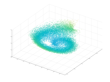
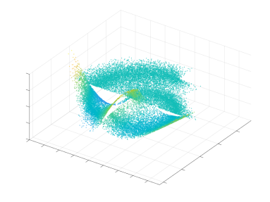
Figure 1. A scaling distribution on the coarsest scale (left) and samplets on level 2 and 3 (second from the left to right).

By construction, samplets satisfy the following properties, which are collected from [24, Theorem 3.6, Lemma 3.9, Theorem 5.4].

Theorem 3.5.

The spaces $\mathcal{X}_{j}$ defined in equation (17) form the desired multiresolution analysis (9), where the corresponding complement spaces $\mathcal{S}_{j}$ from (18) satisfy

$$\mathcal{X}_{j+1}=\mathcal{X}_{j}\overset{\perp}{\oplus}\mathcal{S}_{j}\quad\text{for all}\quad j=0,1,\ldots,J-1.$$

The associated samplet basis $\mathbf{\Sigma}_{N}$ defined in (19) constitutes an orthonormal basis of $\mathcal{X}$ and we have:

1. The number of all samplets on level $j$ behaves like $2^{j}$.

2. The samplets have vanishing moments of order $q+1$, i.e., there holds (12).

3. Each samplet is supported in a specific cluster $\nu$. If the points in $X$ are quasi-uniform, then the diameter of the cluster satisfies $\operatorname{diam}(\nu)\sim 2^{-j_{\nu}/d}$ and there holds (11).

4. The coefficient vector ${\boldsymbol{\omega}}_{j,k}=\big{[}\omega_{j,k,i}\big{]}_{i}$ of the samplet $\sigma_{j,k}$ on the cluster $\nu$ fulfills

   $$\|{\boldsymbol{\omega}}_{j,k}\|_{1}\leq\sqrt{|\nu|}.$$

5. Let $f\in C^{q+1}(\Omega)$. Then, there holds for a samplet $\sigma_{j,k}$ supported on the cluster $\nu$ that

   $$|(f,\sigma_{j,k})_{\Omega}|\leq\bigg{(}\frac{d}{2}\bigg{)}^{q+1}\frac{\operatorname{diam}(\nu)^{q+1}}{(q+1)!}\|f\|_{C^{q+1}(\Omega)}\|{\boldsymbol{\omega}}_{j,k}\|_{1}.$$

Remark 3.6.

Each samplet is a linear combination of the Dirac measures supported at the points in $X$. The related coefficient vectors ${\boldsymbol{\omega}}_{j,k}$ in

(20) $$\sigma_{j,k}=\sum_{i=1}^{N}\omega_{j,k,i}\delta_{{\boldsymbol{x}}_{i}}$$

are pairwise orthonormal with respect to the inner product (2). The dual samplet in $\mathcal{H}_{X}$ is given by

$$\tilde{\sigma}_{j,k}=\sum_{i=1}^{N}\tilde{\omega}_{j,k,i}\kappa({\boldsymbol{x}}_{i},\cdot),\quad\text{where}\quad\tilde{\boldsymbol{\omega}}_{j,k}\mathrel{\mathrel{\mathop{:}}=}{\boldsymbol{K}}^{-1}{\boldsymbol{\omega}}_{j,k},$$

as there holds

$$\langle\tilde{\sigma}_{j,k},\hat{\sigma}_{j^{\prime}k^{\prime}}\rangle_{\mathcal{H}}=(\tilde{\sigma}_{j,k},\sigma_{j^{\prime}k^{\prime}})_{\Omega} =\sum_{i,i^{\prime}=1}^{N}\tilde{\omega}_{j,k,i}{\omega}_{j^{\prime},k^{\prime},i^{\prime}}\big{(}\kappa({\boldsymbol{x}}_{i},\cdot),\delta_{{\boldsymbol{x}}_{i^{\prime}}}\big{)}_{\Omega}$$

$$=\tilde{\boldsymbol{\omega}}_{j,k}^{\intercal}{\boldsymbol{K}}{\boldsymbol{\omega}}_{j^{\prime},k^{\prime}}=\delta_{(j,k),(j^{\prime},k^{\prime})}.$$

3.3. Matrix compression

For the compression of the kernel matrix ${\boldsymbol{K}}$ from (3), with samplets of vanishing moment order $q+1$, with integer $q\geq 0$, we suppose that kernel $\kappa$ is “$q+1$-asymptotically smooth”. This is to say that there are constants $c_{\kappa,\boldsymbol{\alpha},\boldsymbol{\beta}}>0$ such that for all ${\boldsymbol{x}},{\boldsymbol{y}}\in\Omega$ with ${\boldsymbol{x}}\neq{\boldsymbol{y}}$ there holds

(21) $$\bigg{|}\frac{\partial^{|\boldsymbol{\alpha}|+|\boldsymbol{\beta}|}}{\partial{\boldsymbol{x}}^{\boldsymbol{\alpha}}\partial{\boldsymbol{y}}^{\boldsymbol{\beta}}}\kappa({\boldsymbol{x}},{\boldsymbol{y}})\bigg{|}\leq c_{\kappa,\boldsymbol{\alpha},\boldsymbol{\beta}}\|{\boldsymbol{x}}-{\boldsymbol{y}}\|_{2}^{-(|\boldsymbol{\alpha}|+|\boldsymbol{\beta}|)}\quad\text{for all }|\boldsymbol{\alpha}|,|\boldsymbol{\beta}|\leq q+1\;.$$

Note that such an estimate can only be valid for continuous kernels as considered here, but not for singular kernels. However, we observe in passing that this condition is considerably weaker than the notion of asymptotic smoothness of kernels in ${\mathcal{H}}$-matrix theory, cp. [20]. The condition there would correspond to infinite differentiability in (21) with analytic estimates on the constants $c_{\kappa,\boldsymbol{\alpha},\boldsymbol{\beta}}$.

Due to (21), we have in accordance with [24, Lemma 5.3] the decay estimate

(22) $$(\kappa,\sigma_{j,k}\otimes\sigma_{j^{\prime},k^{\prime}})_{\Omega\times\Omega}\leq c_{\kappa,q}\frac{\operatorname{diam}(\nu)^{q+1}\operatorname{diam}(\nu^{\prime})^{q+1}}{\operatorname{dist}(\nu_{j,k},\nu_{j^{\prime},k^{\prime}})^{2(q+1)}}\|{\boldsymbol{\omega}}_{j,k}\|_{1}\|{\boldsymbol{\omega}}_{j^{\prime},k^{\prime}}\|_{1}$$

for two samplets $\sigma_{j,k}$ and $\sigma_{j^{\prime},k^{\prime}}$, with the vanishing moment property of order $q+1$ and supported on the clusters $\nu$ and $\nu^{\prime}$ such that $\operatorname{dist}(\nu,\nu^{\prime})>0$.

Estimate (22) holds for a wide range of kernels that obey the so-called Calderón-Zygmund estimates. It immediately results in the following compression strategy for kernel matrices in samplet representation, cp. [24, Theorem 5.4], which is well-known in the context of wavelet compression of operator equations see, e.g., [41].

Theorem 3.7 ($S$-compression).

Set all coefficients of the kernel matrix

$${\boldsymbol{K}}^{\Sigma}\mathrel{\mathrel{\mathop{:}}=}\big{[}(\kappa,\sigma_{j,k}\otimes\sigma_{j^{\prime},k^{\prime}})_{\Omega\times\Omega}\big{]}_{j,j^{\prime},k,k^{\prime}}$$

to zero which satisfy the $\eta$-admissibility condition

(23) $$\operatorname{dist}(\nu,\nu^{\prime})\geq\eta\max\{\operatorname{diam}(\nu),\operatorname{diam}(\nu^{\prime})\},\quad\eta>0,$$

where $\nu$ is the cluster supporting $\sigma_{j,k}$ and $\nu^{\prime}$ is the cluster supporting $\sigma_{j^{\prime},k^{\prime}}$, respectively.

Then, the resulting S-compressed matrix ${\boldsymbol{K}}^{\eta}$ satisfies

$$\big{\|}{\boldsymbol{K}}^{\Sigma}-{\boldsymbol{K}}^{\eta}\big{\|}_{F}\leq c{\eta^{-2(q+1)}}N\sqrt{\log(N)}.$$

for some constant $c>0$ dependent on the polynomial degree $q$ and the kernel $\kappa$.

Remark 3.8.

We remark that Theorem 3.7 uses the Frobenius norm for measuring the error rather than the operator norm, as it gives control on each matrix coefficient. Estimates with respect to the operator norm would be similar.

The $\eta$-admissibility condition (23) appears reminiscent to the one used for hierarchical matrices, compare, e.g., [10] and the references there. However, in the present context, the clusters $\nu$ and $\nu^{\prime}$ may also be located on different levels, i.e., $j_{\nu}\neq j_{\nu^{\prime}}$ in general. As a consequence, the resulting block cluster tree is the cartesian product $\mathcal{T}\times\mathcal{T}$ rather than the level-wise cartesian product considered in the context of hierarchical matrices.

The error bounds for $S$-compression hold for kernel functions $\kappa$ with finite differentiability (especially, with derivatives of order $q+1$, cp. [24, Lemma 5.3]), as opposed to the usual requirement of asymptotic smoothness which appears in the error analysis of the $\mathcal{H}$-format, see [20] and the references therein.

For point sets $X=\{{\boldsymbol{x}}_{i}\}_{i=1}^{N}$ that are quasi-uniform in the sense of Definition 3.3, there holds

$$\frac{1}{N^{2}}\big{\|}{\boldsymbol{K}}^{\Sigma}\big{\|}_{F}^{2}=\frac{1}{N^{2}}\sum_{i=1}^{N}\sum_{j=1}^{N}|\kappa({\boldsymbol{x}}_{i},{\boldsymbol{x}}_{j})|^{2}\sim\int_{\Omega}\int_{\Omega}|\kappa({\boldsymbol{x}},{\boldsymbol{y}})|^{2}\operatorname{d}\!{\boldsymbol{x}}\operatorname{d}\!{\boldsymbol{y}},$$

i.e., $\big{\|}{\boldsymbol{K}}^{\Sigma}\big{\|}_{F}\sim N$. Thus, we can refine the above result, see also [24, Corollary 5.5].

Corollary 3.9.

In case of quasi-uniform points ${\boldsymbol{x}}_{i}\in X$, the $S$-compressed matrix ${\boldsymbol{K}}^{\eta}$ has only $\mathcal{O}(N\log N)$ nonzero coefficients, while it satisfies the error estimate

(24) $$\frac{\big{\|}{\boldsymbol{K}}^{\Sigma}-{\boldsymbol{K}}^{\eta}\big{\|}_{F}}{\big{\|}{\boldsymbol{K}}^{\Sigma}\big{\|}_{F}}\leq c\eta^{-2(q+1)}\sqrt{\log N}.$$

In [24], an algorithm has been proposed which computes the compressed matrix ${\boldsymbol{K}}^{\eta}$ in work and memory $\mathcal{O}(N\log N)$. The key ingredient to achieve this is the use of an interpolation-based fast multipole method and $\mathcal{H}^{2}$-matrix techniques [10, 19, 3].

4. Samplet matrix algebra

4.1. Addition and multiplication

To bound the cost for the addition of two compressed kernel matrices represented with respect to the same cluster tree, it is sufficient to assume that the points in $X$ are quasi-uniform. Then it is straightforward to see that the cost for adding such matrices is $\mathcal{O}({N\log N})$. The multiplication of two compressed matrices, in turn, is motivated by concatenation $\mathcal{C}=\mathcal{A}\circ\mathcal{B}$ of the two pseudodifferential operators $\mathcal{A}$ and $\mathcal{B}$. In suitable algebras, the product $\mathcal{C}$ is again a pseudodifferential operator and, hence, compressible. The respective kernel $\kappa_{\mathcal{C}}(\cdot,\cdot)$ is given by

(25) $$\kappa_{\mathcal{C}}({\boldsymbol{x}},{\boldsymbol{y}})=\int_{\Omega}\kappa_{\mathcal{A}}({\boldsymbol{x}},{\boldsymbol{z}})\kappa_{\mathcal{B}}({\boldsymbol{z}},{\boldsymbol{y}})\operatorname{d}\!{\boldsymbol{z}}.$$

Since $\Omega\subset\mathbb{R}^{d}$ is bounded by assumption, we may without loss of generality assume $\Omega\subset[0,1)^{d}$. Then, if the distribution of the data points in $X=\{\boldsymbol{x}_{i}\}_{i=1}^{N}\subset\Omega$ satisfies the stronger assumption of being asymptotically uniform modulo one, then there holds

(26) $$\lim_{N\to\infty}\frac{|\Omega|}{N}\sum_{i=1}^{N}(f,\delta_{{\boldsymbol{x}}_{i}})_{\Omega}=\int_{\Omega}f({\boldsymbol{x}})\operatorname{d}\!{\boldsymbol{x}}$$

for every Riemann integrable function $f\colon\Omega\to\mathbb{R}$, cp. [39]. Hence, we may interpret the matrix product as a discrete version of the convolution (25). In view of (26), we conclude

(27) $$\bigg{|}\kappa_{\mathcal{C}}({\boldsymbol{x}},{\boldsymbol{y}})-\frac{|\Omega|}{N}\sum_{k=1}^{N}\kappa_{\mathcal{A}}({\boldsymbol{x}},{\boldsymbol{x}}_{k})\kappa_{\mathcal{B}}({\boldsymbol{x}}_{k},{\boldsymbol{y}})\bigg{|}\to 0\ \text{as $N\to\infty$}.$$

Consequently, the product of two kernel matrices

$$\boldsymbol{K}_{\mathcal{A}}=[\kappa_{\mathcal{A}}(\boldsymbol{x}_{i},\boldsymbol{x}_{j})]_{i,j=1}^{N},\quad\boldsymbol{K}_{\mathcal{B}}=[\kappa_{\mathcal{B}}(\boldsymbol{x}_{i},\boldsymbol{x}_{j})]_{i,j=1}^{N}$$

yields an $S$-compressible matrix $\boldsymbol{K}_{\mathcal{A}}\cdot\boldsymbol{K}_{\mathcal{B}}\in\mathbb{R}^{N\times N}$.

Theorem 4.1.

Let $X=\{\boldsymbol{x}_{i}\}_{i=1}^{N}\subset\Omega$ be asymptotically distributed uniformly modulo one, cp. (26), and denote by $\boldsymbol{K}_{\mathcal{C}}$ the corresponding kernel matrix

$$\boldsymbol{K}_{\mathcal{C}}=\frac{N}{|\Omega|}[\kappa_{\mathcal{C}}(\boldsymbol{x}_{i},\boldsymbol{x}_{j})]_{i,j=1}^{N}$$

with $\kappa_{\mathcal{C}}(\cdot,\cdot)$ from (25). Then, there holds

$$\frac{\|\boldsymbol{K}_{\mathcal{C}}-\boldsymbol{K}_{\mathcal{A}}\boldsymbol{K}_{\mathcal{B}}\|_{F}}{\|\boldsymbol{K}_{\mathcal{C}}\|_{F}}\to 0\ \text{as $N\to\infty$}.$$

Proof.

On the one hand, we conclude from (27) that, as $N\to\infty$,

$$\|\boldsymbol{K}_{\mathcal{C}}-\boldsymbol{K}_{\mathcal{A}}\boldsymbol{K}_{\mathcal{B}}\|_{F}^{2} =\sum_{i,j=1}^{N}\bigg{[}\frac{N}{|\Omega|}\kappa_{\mathcal{C}}({\boldsymbol{x}}_{i},{\boldsymbol{x}}_{j})-\sum_{k=1}^{N}\kappa_{\mathcal{A}}({\boldsymbol{x}}_{i},{\boldsymbol{z}}_{k})\kappa_{\mathcal{B}}({\boldsymbol{z}}_{k},{\boldsymbol{x}}_{j})\bigg{]}^{2}$$

$$\sim N^{4}\int_{\Omega}\int_{\Omega}\bigg{[}\kappa_{\mathcal{C}}({\boldsymbol{x}},{\boldsymbol{y}})-\frac{|\Omega|}{N}\sum_{k=1}^{N}\kappa_{\mathcal{A}}({\boldsymbol{x}},{\boldsymbol{x}}_{k})\kappa_{\mathcal{B}}({\boldsymbol{x}}_{k},{\boldsymbol{y}})\bigg{]}^{2}\operatorname{d}\!\boldsymbol{x}\operatorname{d}\!\boldsymbol{y}$$

$$=o(N^{4}).$$

On the other hand, we find likewise

$$\|\boldsymbol{K}_{\mathcal{C}}\|_{F}^{2}\sim\int_{\Omega}\int_{\Omega}N^{2}\kappa_{\mathcal{C}}({\boldsymbol{x}},{\boldsymbol{y}})^{2}\operatorname{d}\!\boldsymbol{x}\operatorname{d}\!\boldsymbol{y}\sim N^{4}.$$

This implies the assertion. ∎

Remark 4.2.

We mention that the consistency bound in the preceding theorem is rather crude. Under provision of stronger kernel-function regularity, corresponding higher convergence rates can be achieved, given that $X$ satisfies appropriate higher-order quasi-Monte Carlo designs, see, e.g., [11] and the references there.

Let $\boldsymbol{K}_{\mathcal{A}}^{\eta},\boldsymbol{K}_{\mathcal{B}}^{\eta},\boldsymbol{K}_{\mathcal{C}}^{\eta}$ be compressed with respect to the same compression pattern. We assume for given $\varepsilon(\eta)>0$ that $\eta$ in (24) is chosen such that

$$\big{\|}{\boldsymbol{K}}^{\Sigma}-{\boldsymbol{K}}^{\eta}\big{\|}_{F}\leq\varepsilon(\eta){\big{\|}{\boldsymbol{K}}^{\Sigma}\big{\|}_{F}},\quad\text{for }{\boldsymbol{K}}\in\{\boldsymbol{K}_{\mathcal{A}},\boldsymbol{K}_{\mathcal{B}},\boldsymbol{K}_{\mathcal{C}}\}.$$

Then, a repeated application of the triangle inequality yields

$$\|\boldsymbol{K}_{\mathcal{C}}^{\eta}-\boldsymbol{K}_{\mathcal{A}}^{\eta}\boldsymbol{K}_{\mathcal{B}}^{\eta}\|_{F}$$

$$\quad\leq\|\boldsymbol{K}_{\mathcal{C}}^{\Sigma}-\boldsymbol{K}_{\mathcal{C}}^{\eta}\|_{F}+\|\boldsymbol{K}_{\mathcal{A}}^{\Sigma}\|_{F}\|\boldsymbol{K}_{\mathcal{B}}^{\Sigma}-\boldsymbol{K}_{\mathcal{B}}^{\eta}\|_{F}+\|\boldsymbol{K}_{\mathcal{B}}^{\eta}\|_{F}\|\boldsymbol{K}_{\mathcal{A}}^{\Sigma}-\boldsymbol{K}_{\mathcal{A}}^{\eta}\|_{F}$$

$$\quad\leq\varepsilon(\eta)\big{(}\|\boldsymbol{K}_{\mathcal{C}}\|_{F}+\|\boldsymbol{K}_{\mathcal{A}}\|_{F}\|\boldsymbol{K}_{\mathcal{B}}\|_{F}+\big{(}1+\varepsilon(\eta)\big{)}\|\boldsymbol{K}_{\mathcal{A}}\|_{F}\|\boldsymbol{K}_{\mathcal{B}}\|_{F}\big{)}$$

$$\quad\lesssim\varepsilon(\eta)\big{(}\|\boldsymbol{K}_{\mathcal{C}}\|_{F}+\|\boldsymbol{K}_{\mathcal{A}}\|_{F}\|\boldsymbol{K}_{\mathcal{B}}\|_{F}\big{)}.$$

This means that we only need to compute $\mathcal{O}(N\log N)$ matrix entries to determine an approximate version $(\boldsymbol{K}_{\mathcal{A}}^{\eta}\boldsymbol{K}_{\mathcal{B}}^{\eta})^{\eta}$ of the product $\boldsymbol{K}_{\mathcal{A}}^{\eta}\cdot\boldsymbol{K}_{\mathcal{B}}^{\eta}$. We like to stress that this formatted matrix multiplication is exact on the given compression pattern. The next theorem gives a cost bound on the matrix multiplication.

Theorem 4.3.

Consider two kernel matrices

$$\boldsymbol{K}_{\mathcal{A}}^{\eta}=[a_{(j,k),(j^{\prime},k^{\prime})}],\quad\boldsymbol{K}_{\mathcal{B}}^{\eta}=[b_{(j,k),(j^{\prime},k^{\prime})}]\in\mathbb{R}^{N\times N}$$

in samplet representation which are $S$-compressed with respect to the compression pattern induced by the $\eta$-admissibility condition (23).

Then, computing with respect to the same compression pattern the matrix $\boldsymbol{K}_{\mathcal{C}}^{\eta}=[c_{(j,k),(j^{\prime},k^{\prime})}]\in\mathbb{R}^{N\times N}$, where the nonzero entries are given by the discrete inner product

(28) $$c_{(j,k),(j^{\prime},k^{\prime})}=\sum_{\ell=0}^{J}\sum_{m\in\nabla_{\ell}}a_{(j,k),(\ell,m)}b_{(\ell,m),(j^{\prime},k^{\prime})},$$

is of cost $\mathcal{O}(N\log^{2}N)$.

Proof.

To estimate the cost of the matrix multiplication, we shall make use of the compression rule (23). We assume for all clusters that $\operatorname{diam}(\nu)\sim 2^{-j/d}$ if $\nu$ is on level $j$. Thus, the samplet $\sigma_{j,k}$ has approximately the diameter $2^{-j/d}$ and, therefore, only $\mathcal{O}(2^{\ell-j})$ samplets $\sigma_{\ell,m}$ of diameter $\sim 2^{-\ell/d}$ are found in its nearfield if $\ell\geq j$ while only $\mathcal{O}(1)$ are found if $\ell<j$. For fixed level $0\leq\ell\leq J$ in (28), we thus have at most $\mathcal{O}(\max\{2^{\ell-\max\{j,j^{\prime}\}},1\})$ nonzero products to evaluate per coefficient $c_{(j,k),(j^{\prime},k^{\prime})}$. We assume without loss of generality that $j\geq j^{\prime}$ and sum over $\ell$, which yields the cost $\mathcal{O}(\max\{2^{J-j},j\})$. Per target block matrix ${\boldsymbol{C}}_{j,j^{\prime}}=[c_{(j,k),(j^{\prime},k^{\prime})}]_{j,j^{\prime}}$, we have $\mathcal{O}(2^{\max\{j,j^{\prime}\}})=\mathcal{O}(2^{j})$ nonzero coefficients. Hence, the cost for computing the desired target block is $\mathcal{O}(2^{j}\max\{2^{J-j},j\})$. We shall next sum over $j$ and $j^{\prime}$

$$\sum_{j=0}^{J}\sum_{j^{\prime}=0}^{j}\mathcal{O}(2^{j}\max\{2^{J-j},j\}) =\sum_{j=0}^{J}\sum_{j^{\prime}=0}^{j}\mathcal{O}(\max\{N,j2^{j}\})$$

$$=\sum_{j=0}^{J}\mathcal{O}(j\max\{N,j2^{j}\})$$

$$=\mathcal{O}(N\log^{2}N).$$

∎

4.2. Sparse selected inversion

Having addition and multiplication of kernel matrices at our disposal, we consider the matrix inversion next. To this end, observe that the inverse ${\mathcal{A}}^{-1}$ of a pseudodifferential operator ${\mathcal{A}}$ from a suitable algebra of pseudodifferential operators, provided that it exists, is again a pseudodifferential operator, see Section A. However, if ${\mathcal{A}}$ is a pseudodifferential operator of negative order as in the present RKHS case, the operator ${\mathcal{A}}^{-1}$ is of positive order and hence gives rise to a singular kernel which does not satisfy the condition (21). Even so, in the regime of kernel matrices we are rather interested in inverting regularized pseudodifferential operators, i.e., ${\mathcal{A}}+\mu{I}$, where $I$ denotes the identity. For such operators, we have the following lemma.

Lemma 4.4.

Let ${\mathcal{A}}$ be a pseudodifferential operator of order $s\leq 0$ with symmetric and positive semidefinite kernel function.

Then, for any $\mu>0$, the inverse of ${\mathcal{A}}+\mu{I}$ can be decomposed into $\frac{1}{\mu}{I}-{\mathcal{B}}$ with

(29) $${\mathcal{B}}=\frac{1}{\mu}({\mathcal{A}}+\mu{I})^{-1}{\mathcal{A}}.$$

Especially, ${\mathcal{B}}$ is also a pseudodifferential operator of order $s$, which admits a symmetric and positive semidefinite kernel function.

Proof.

In view of (29), we infer that

$$({\mathcal{A}}+\mu{I})\bigg{(}\frac{1}{\mu}{I}-{\mathcal{B}}\bigg{)}=\frac{1}{\mu}{\mathcal{A}}+I-({\mathcal{A}}+\mu{I}){\mathcal{B}}=I+\frac{1}{\mu}{\mathcal{A}}-\frac{1}{\mu}{\mathcal{A}}=I.$$

Therefore, $\frac{1}{\mu}{I}-{\mathcal{B}}$ is the inverse operator to ${\mathcal{A}}+\mu{I}$. Since ${\mathcal{A}}+\mu{I}$ is of order 0, $({\mathcal{A}}+\mu{I})^{-1}$ is of order 0, too, and thus $({\mathcal{A}}+\mu{I})^{-1}{\mathcal{A}}$ is of the same order as ${\mathcal{A}}$. Finally, the symmetry and nonnegativity of $\mathcal{B}$ follows from the symmetry and nonnegativity of $\mathcal{A}$. ∎

As a consequence of this lemma, the inverse $({\boldsymbol{K}}_{\mathcal{A}}+\mu{\boldsymbol{I}})^{-1}\in\mathbb{R}^{N\times N}$ of the associated kernel matrix ${\boldsymbol{K}}_{\mathcal{A}}+\mu{\boldsymbol{I}}\in\mathbb{R}^{N\times N}$ is $S$-compressible with respect to the same compression pattern as ${\boldsymbol{K}}_{\mathcal{A}}$. In [23], strong numerical evidence was presented that a sparse Cholesky factorization of a compressed kernel matrix can efficiently be computed by means of nested dissection, cf. [17]. This suggests the computation of the inverse $({\boldsymbol{K}}_{\mathcal{A}}+\mu{\boldsymbol{I}})^{-1}$ in samplet basis on the compression pattern of ${\boldsymbol{K}}_{\mathcal{A}}$ by means of selective inversion [37] of a sparse matrix. The approach is outlined below.

Assume that ${\boldsymbol{A}}\in\mathbb{R}^{N\times N}$ is symmetric and positive definite. There are two steps in the inversion algorithm. The first stage involves factorizing the input matrix $\boldsymbol{A}$ into $\boldsymbol{A}=\boldsymbol{LDL}^{\intercal}$. The $\boldsymbol{L}$ and $\boldsymbol{D}$ matrices are used in the second phase to compute the selected components of $\boldsymbol{A}^{-1}$. The first step will be referred to as factorization in the following and the second step as selected inversion. To explain the second step, let ${\boldsymbol{A}}$ be partitioned according to

$${\boldsymbol{A}}=\begin{bmatrix}{\boldsymbol{A}}_{11}&{\boldsymbol{A}}_{12}\\ {\boldsymbol{A}}_{12}^{\intercal}&{\boldsymbol{A}}_{22}\end{bmatrix}.$$

In particular, the diagonal blocks ${\boldsymbol{A}}_{ii}$ are also symmetric and positive definite. The selected inversion is based on the identity

(30) $${\boldsymbol{A}}^{-1}=\begin{bmatrix}{\boldsymbol{A}}_{11}^{-1}+{\boldsymbol{C}}{\boldsymbol{S}}^{-1}{\boldsymbol{C}}^{\intercal}&{\boldsymbol{C}}{\boldsymbol{S}}^{-1}\\ {\boldsymbol{S}}^{-1}{\boldsymbol{C}}^{\intercal}&{\boldsymbol{S}}^{-1}\end{bmatrix},$$

where ${\boldsymbol{S}}\mathrel{\mathrel{\mathop{:}}=}{\boldsymbol{A}}_{22}+{\boldsymbol{A}}_{12}^{\intercal}{\boldsymbol{C}}$ is the Schur complement with ${\boldsymbol{C}}\mathrel{\mathrel{\mathop{:}}=}-{\boldsymbol{A}}_{11}^{-1}{\boldsymbol{A}}_{12}$. For sparse matrices, this block algorithm can efficiently be realized based on the observation that for the computation of the entries of ${\boldsymbol{A}}^{-1}$ on the pattern of ${\boldsymbol{L}}$ only the entries on the pattern of ${\boldsymbol{L}}$ are required, as it is well known from the sparse matrix literature, cp. [37, 13, 18]. We note that the pattern of ${\boldsymbol{A}}$ is particularly contained in the pattern of ${\boldsymbol{L}}$.

4.3. Algorithmic aspects

A block selected inversion algorithm has at least two advantages: Because $\boldsymbol{A}$ is sparse, blocks can be specified in terms of supernodes [37]. This allows us to use level-3 BLAS to construct an efficient implementation by leveraging memory hierarchy in current microprocessors. A supernode is a group of nodes with the same nonzero structure below the diagonal in their respective columns (of their $\boldsymbol{L}$ factor). The supernodal approach for sparse symmetric factorization represents the factor $\boldsymbol{L}$ as a set of supernodes, each of which consists of a contiguous set of $\boldsymbol{L}$ columns with identical nonzero patterns, and each supernode is stored as a dense submatrix to take advantage of level-3 BLAS calculations.

Taking these consideration as a starting point, it is natural to employ the selected inversion approach presented in [53] and available in [43] in order to directly compute the entries on the pattern of the inverse matrix. For the particular implementation of the selected inversion, we rely on Pardiso. For larger kernel matrices, which cannot be indexed by $32bit$ integers due to the comparatively large number of non-zero entries, we combine the selected inversion with a divide and conquer approach based on the identity (30). The inversion of the ${\boldsymbol{A}}_{11}$ block and of the Schur complement ${\boldsymbol{S}}$ are performed with Pardiso (exploiting symmetry), while the other arithmetic operations, i.e., addition and multiplication, are performed in a formatted way, compare Theorem 4.3.

4.4. Matrix functions

Based on the $S$-formatted multiplication and inversion of operators represented in samplet basis, certain holomorphic functions of an $S$-compressed operator also admit $S$-formatted approximations with, essentially, corresponding approximation accuracies.

To illustrate this, we recall the method in [22]. This approach employs the contour integral representation

(31) $$f({\boldsymbol{A}})=\frac{1}{2\pi i}\int_{\Gamma}f(z)(z{\boldsymbol{I}}-{\boldsymbol{A}})^{-1}\operatorname{d}\!z,$$

where $\Gamma$ is a closed contour being contained in the analyticity region of $f$ and winding once around the spectrum $\sigma({\boldsymbol{A}})$ in counterclockwise direction. As is well-known, analytic functions $f$ of elliptic, self-adjoint pseudodifferential operators yield again pseudodifferential operators in the same algebra, see, e.g., [50, Chap.XII.1]. Hence, ${\boldsymbol{B}}\mathrel{\mathrel{\mathop{:}}=}f({\boldsymbol{A}})$ is $S$-compressible provided that $f$ is analytic. Especially, the $S$-compressed representation $\big{(}f({\boldsymbol{A}}^{\eta})\big{)}^{\eta}$ satisfies

(32) $$\big{\|}{\boldsymbol{B}}^{\Sigma}-\big{(}f({\boldsymbol{A}}^{\eta})\big{)}^{\eta}\big{\|}_{F} \leq\|{\boldsymbol{B}}^{\Sigma}-{\boldsymbol{B}}^{\eta}\|_{F}+\big{\|}\big{(}f({\boldsymbol{A}}^{\Sigma})-f({\boldsymbol{A}}^{\eta})\big{)}^{\eta}\big{\|}_{F}$$

$$\leq\varepsilon\|{\boldsymbol{B}}\|_{F}+L\|{\boldsymbol{A}}^{\Sigma}-{\boldsymbol{A}}^{\eta}\|_{F}$$

$$\leq\varepsilon\big{(}\|{\boldsymbol{B}}\|_{F}+L\|{\boldsymbol{A}}\|_{F}\big{)}.$$

Herein, $L$ denotes the Lipschitz constant of the function $f$. In other words, estimate (32) implies that the error of the approximation of the $S$-formatted matrix function $\big{(}f({\boldsymbol{A}}^{\eta})\big{)}^{\eta}$ is rigorously controlled by the sum of the input error $\|{\boldsymbol{A}}^{\Sigma}-{\boldsymbol{A}}^{\eta}\|_{F}$ and the compression error for the exact output $\|{\boldsymbol{B}}^{\Sigma}-{\boldsymbol{B}}^{\eta}\|_{F}$. The latter is under control if the underlying pseudodifferential operator is of order $s<-d$ since then the kernel is continuous and satisfies (21). In the other cases, some analysis is needed to control this error (see below).

For the numerical approximation of the contour integral (31), one has to apply an appropriate quadrature formula. Exemplarily, we consider the matrix square root, i.e., $f(z)=\sqrt{z}$ for ${\rm Re}z>0$. This occurs for example in the efficient path simulation of Gaussian processes in spatial statistics. We shall here apply, see [22, Eq. (4.4) and comments below], the approximation

(33) $${\boldsymbol{A}}^{-1/2}\approx\frac{2E\sqrt{\underline{c}}}{\pi K}\sum_{k=1}^{K}\frac{\operatorname{dn}\left(t_{k}|1-\varkappa_{\boldsymbol{A}}\right)}{\operatorname{cn}^{2}\left(t_{k}|1-\varkappa_{\boldsymbol{A}}\right)}\left({\boldsymbol{A}}+w_{k}^{2}{\boldsymbol{I}}\right)^{-1},\quad{\boldsymbol{A}}^{1/2}={\boldsymbol{A}}\cdot{\boldsymbol{A}}^{-1/2}.$$

Here, $\operatorname{sn},\operatorname{cn}$ and $\operatorname{dn}$ are the Jacobian elliptic functions [2, Chapter 16], $E$ is the complete elliptic integral of the second kind associated with the parameter $\varkappa_{\boldsymbol{A}}:=\underline{c}/\overline{c}$ [2, Chapter 17], and, for $k\in\{1,\ldots,K\}$,

$$w_{k}\mathrel{\mathrel{\mathop{:}}=}\sqrt{\underline{c}}\,\frac{\operatorname{sn}\left(t_{k}|1-\varkappa_{\boldsymbol{A}}\right)}{\operatorname{cn}\left(t_{k}|1-\varkappa_{\boldsymbol{A}}\right)}\quad\text{and}\quad t_{k}\mathrel{\mathrel{\mathop{:}}=}\frac{E}{K}\big{(}k-\tfrac{1}{2}\big{)}.$$

The quadrature approximation (33) of the contour integral (31) for the matrix square root is known to converge root-exponentially (e.g. [8, Lemma 3.4]) in the number $K$ of quadrature nodes in (33) of the contour integral. Hence, approximate representations to algebraic with respect to $N$ consistency orders can be achieved with $K\sim|\varepsilon(\eta)|$, resulting in overall log-linear complexity of numerical realization of (33) in $S$-format. We also remark that the quadrature shifts $w_{k}^{2}$ in the inversions which occur in (33) act as regularizing “nuggets” of a possibly ill-conditioned ${\boldsymbol{A}}$. The input parameters $0<\underline{c}<\overline{c}$ shall provide bounds to the spectrum of ${\boldsymbol{A}}$, i.e., $\underline{c}\approx\lambda_{\min}({\boldsymbol{A}})$ and $\overline{c}\approx\lambda_{\max}({\boldsymbol{A}})$. Note that we also assume here that ${\boldsymbol{A}}$ is symmetric and positive definite. Moreover, we should mention that, except for the quadrature error, (33) computes the square root $({\boldsymbol{A}}^{\eta})^{-1/2}$ of the compressed input ${\boldsymbol{A}}^{\eta}$ in an exact way on the compression pattern when we use the selected inversion algorithm from Subsection 4.2.

That $({\boldsymbol{A}}^{\eta})^{-1/2}$ is indeed $S$-compressible is a consequence of the following lemma.

Lemma 4.5.

Let ${\mathcal{A}}$ be a pseudodifferential operator of order $s\leq 0$ with symmetric and positive semidefinite kernel function. Then, for any $\mu>0$, the inverse square root of ${\mathcal{A}}+\mu{I}$ can be written as $\frac{1}{\sqrt{\mu}}{I}-{\mathcal{B}}$ with ${\mathcal{B}}$ being also a pseudodifferential operator of order $s$, which admits a symmetric and positive semidefinite kernel function.

Proof.

Straightforward calculation shows that the ansatz

(34) $$(\mathcal{A}+\mu I)^{-1/2}=\frac{1}{\sqrt{\mu}}I-\mathcal{B}$$

is equivalent to

$$(\mathcal{A}+\mu I)\bigg{(}\frac{1}{\mu}I-\frac{2}{\sqrt{\mu}}\mathcal{B}+\mathcal{B}^{2}\bigg{)}=I.$$

Thus,

$$\mathcal{B}\bigg{(}\frac{2}{\sqrt{\mu}}I-\mathcal{B}\bigg{)}=\frac{1}{\mu}(\mathcal{A}+\mu I)^{-1}\mathcal{A},$$

which in view of (34) is equivalent to

$$\mathcal{B}\bigg{(}\frac{1}{\sqrt{\mu}}I+(\mathcal{A}+\mu I)^{-1/2}\bigg{)}=\frac{1}{\mu}\mathcal{A}(\mathcal{A}+\mu I)^{-1}.$$

As both, $\frac{1}{\sqrt{\mu}}I+(\mathcal{A}+\mu I)^{-1/2}$ and $(\mathcal{A}+\mu I)^{-1}$, are pseudodifferential of order 0, $\mathcal{B}$ must have the same order as $\mathcal{A}$. ∎

An alternative to the contour integral for computing the matrix exponential of a (possibly singular) matrix ${\boldsymbol{A}}$ is given by the direct evaluation of the power series

$$\exp({\boldsymbol{A}})=\sum_{k=0}^{\infty}\frac{1}{k!}{\boldsymbol{A}}^{k}.$$

As we show in the numerical results, this series converges very fast for the present matrices under consideration which stem from reproducing kernels, since they correspond to compact operators.

5. Numerical results

The computations in this section have been performed on a single node with two Intel Xeon E5-2650 v3 @2.30GHz CPUs and up to 512GB of main memory. To achieve consistent timings, all computations have been carried out using 16 cores. The samplet compression is implemented in C++11 and relies on the Eigen template library for linear algebra operations. Moreover, the selected inversion is performed by Pardiso. Throughout this section, we employ samplets with $q+1=4$ vanishing moments. The parameter for the admissibility condition (23) is set to $\eta=1.25$. Together with the a priori pattern, which is obtained by neglecting admissible blocks, we also consider an a posteriori compression by setting all matrix entries smaller than $\tau=10^{-5}/N$ to zero resulting in the a posteriori pattern.

5.1. $\boldsymbol{S}$-formatted matrix multiplication

To benchmark the multiplication, we consider uniformly distributed random points on the unit hypercube $[0,1]^{d}$. As kernel, we consider the exponential kernel (which is the Matérn kernel with smoothness parameter $\nu=1/2$ and correlation length $\ell=1$)

(35) $$\kappa({\boldsymbol{x}},{\boldsymbol{y}})=\frac{1}{N}e^{-\|{\boldsymbol{x}}-{\boldsymbol{y}}\|_{2}}$$

Note that we impose the scaling $1/N$ of the kernel function in order fix the largest eigenvalue of the kernel matrix as its trace stays uniformly bounded.

We compute the matrix product ${\boldsymbol{K}}^{\eta}\cdot\tilde{\boldsymbol{K}}^{\eta}$, where $\tilde{\boldsymbol{K}}^{\eta}$ is obtained from ${\boldsymbol{K}}^{\eta}$ by relatively perturbing each nonzero entry by 10% additive noise, which is uniformly distributed in $[0,1]$. This way, we rule out symmetry effects as $\tilde{\boldsymbol{K}}^{\eta}$ will not be symmetric in general.

Figure 2. Computation times for matrix multiplication (left) and multiplication errors (right).

To measure the multiplication error, we consider the estimator

$$e_{F}({\boldsymbol{A}})\mathrel{\mathrel{\mathop{:}}=}\frac{\|{\boldsymbol{A}}{\boldsymbol{X}}\|_{F}}{\|{\boldsymbol{X}}\|_{F}},$$

where ${\boldsymbol{X}}\in\mathbb{R}^{N\times 10}$ is a random matrix with uniformly distributed independent entries. The left hand side of Figure 2 shows the computation time for a single multiplication. The dashed lines correspond to the asymptotic rates $\mathcal{O}(N\log^{\alpha}N)$ for $\alpha=0,1,2,3$. It can be seen that the multiplication time for $d=2$ perfectly reflects the expected essentially linear behavior. Though the graph is steeper for $d=3$, we expect it to flatten further for larger $N$. The right hand side of the plot shows the multiplication error $e_{F}({\boldsymbol{K}}^{\eta}\cdot\tilde{\boldsymbol{K}}^{\eta}-{\boldsymbol{K}}^{\eta}\boxdot\tilde{\boldsymbol{K}}^{\eta})$, where the formatted multiplication $\boxdot$ is performed on the a posteriori pattern. Taking into account that the compression errors for ${\boldsymbol{K}}^{\eta}$ are approximately $5.6\cdot 10^{-6}$ for $d=2$ and $1.6\cdot 10^{-5}$ for $d=3$, the obtained matrix product can be considered to be very accurate.

5.2. $\boldsymbol{S}$-formatted matrix inversion

In order to assess the numerical performance of the matrix inversion, we again consider uniformly distributed random points on the unit hypercube $[0,1]^{d}$. Since the separation radius $q_{X}$ ranges between $4.7\cdot 10^{-5}$ ($N=5000$) and $2.8\cdot 10^{-7}$ ($N=1\,0000\,000$) for $d=2$ and $3.8\cdot 10^{-4}$ ($N=5000$) and $3.2\cdot 10^{-5}$ ($N=1\,0000\,000$) for $d=3$, we do not expect that ${\boldsymbol{K}}^{\eta}$ to be invertible. Therefore, we rather consider the regularized version ${\boldsymbol{K}}^{\eta}+\mu{\boldsymbol{I}}$ for a ridge parameter $\mu>0$.

As our theoretical results suggest that the inverse has the same a priori pattern as the matrix itself, we first consider the inversion on the a priori pattern for $d=2$.

Figure 3. Results for $d=2$. Left panel: Computation times for compressed matrix assembly and selected inversion on the a priori pattern. Dashed lines indicate linear ($\alpha=1$) and super-linear ($\alpha=1.5$) scaling, respectively. Right panel: Inversion errors for ridge parameters $\mu=10^{-6},10^{-4},10^{-2}$.

The left hand side of Figure 3 shows the computation times for the inverse matrix employing Pardiso. The dashed line shows the asymptotic rates $\mathcal{O}(N^{\alpha})$ for $\alpha=1,1.5$. For $N=1\,000\,000$, due to the large amount of non-zero entries, we use the block inversion with one subdivision. This explains the bump in the computation time due to the formatted matrix multiplication. Besides this, Pardiso perfectly exhibits the expected rate of $N^{1.5}$. The right hand side of the plot shows the error $e_{F}\big{(}({\boldsymbol{K}}^{\eta}+\mu{\boldsymbol{I}})^{\framebox{\text{\tiny$-\!1$}}}({\boldsymbol{K}}^{\eta}+\mu{\boldsymbol{I}})-{\boldsymbol{I}}\big{)}$ for the ridge parameters $\mu=10^{-6},10^{-4},10^{-2}$, where ${}^{\framebox{\text{\tiny$-\!1$}}}$ denotes the selected in version on the pattern of ${\boldsymbol{K}}^{\eta}$. As expected, the error reduces significantly with increasing ridge parameter.

As the a priori pattern typically exhibits significantly less entries, we also investigate the inversion on the a posteriori pattern. The corresponding results are shown in Figure 4

Figure 4. Results for $d=2$. Left panel: Computation times for compressed matrix assembly and selected inversion on the a posteriori pattern. Dashed lines indicate linear ($\alpha=1$) and super-linear ($\alpha=1.5$) scaling, respectively. Right panel: Inversion errors for ridge parameters $\mu=10^{-6},10^{-4},10^{-2}$.

As can be seen on the left hand side of the figure, the selected inversion now even exhibits a linear behavior, which is explained by the fixed threshold $\tau$, resulting in successively less entries for increasing $N$. On the other hand, the errors for the different ridge parameters, depicted on the right hand side of the same figure, asymptotically exhibit the same behavior as in the a priori case.

Figure 5. Results for $d=3$. Left panel: Computation times for compressed matrix assembly and selected inversion on the a posteriori pattern. Dashed lines indicate linear ($\alpha=1$) and quadratic ($\alpha=2$) scaling, respectively.

Right panel: Inversion errors for ridge parameters $\mu=10^{-6},10^{-4},10^{-2}$.

Motivated by the results for $d=2$, we consider only the inversion on the a posteriori pattern for $d=3$. The corresponding results are shown in Figure 5. On the left hand side of the figure, again the computation times are shown. The dashed lines show the asymptotic rates $\mathcal{O}(N^{\alpha})$ for $\alpha=1,2$. Until $N=100\,000$, the expected quadratic rate is perfectly matched. Due to the large number of non-zeros in the case $d=3$, we have employed the block inversion with three recursion steps for $N>100\,000$, resulting in the peculiar linear behavior for the respective values in the graph. The errors depicted on the right hand side show a behavior similar to the case $d=2$, with a slightly reduced decay.

5.3. $\boldsymbol{S}$-formatted matrix functions

We compute the matrix square root ${\boldsymbol{A}}^{1/2}$ and the matrix exponential $\exp({\boldsymbol{A}})$ for the exponential kernel

$$\kappa({\boldsymbol{x}},{\boldsymbol{y}})=\frac{1}{N}e^{-2\|{\boldsymbol{x}}-{\boldsymbol{y}}\|_{2}}$$

This time, the data points are randomly subsampled from from a 3D scan of the head of Michelangelo’s David (The scan is provided by the Statens Museum for Kunst under the Creative Commons CC0 license), cp. Figure 6.

Figure 6. Data points from a 3D scan of the head of Michelangelo’s David. The scan is provided by the Statens Museum for Kunst under the Creative Commons CC0 license.

The bounding box of the bunny is $[-0.52,0.42]\times[-0.47,0.46]\times[-0.18,0.78]$. All other parameters are set as in the examples before. Moreover, we set the ridge parameter to $\mu=10^{-4}$. The smallest eigenvalue is estimated by the ridge parameter, while the largest eigenvalue is upper bounded by $1$. For the contour integral method for the computation of the matrix square root, we found stagnation in the error for $K\geq 7$ quadrature points. The corresponding errors $e_{F}\big{(}({\boldsymbol{K}}^{\eta}+\mu{\boldsymbol{I}})^{\framebox{\text{\tiny$1/2$}}}({\boldsymbol{K}}^{\eta}+\mu{\boldsymbol{I}})^{\framebox{\text{\tiny$1/2$}}}-({\boldsymbol{K}}^{\eta}+\mu{\boldsymbol{I}})\big{)}$ for different values of $N$ are tabulated in Table 1

$N$	$5\,000$	$10\,000$	$50\,000$	$100\,000$	$234\,553$
$e_{F}$	$1.43\cdot 10^{-3}$	$7.68\cdot 10^{-4}$	$3.90\cdot 10^{-4}$	$2.82\cdot 10^{-4}$	$3.59\cdot 10^{-4}$

Table 1. Errors for the contour integral method for $({\boldsymbol{K}}^{\eta}+\mu{\boldsymbol{I}})^{1/2}$.

Finally, Table 2 shows the approximation error $e_{F}\big{(}\exp({\boldsymbol{K}}^{\eta})-\boxed{\exp}({\boldsymbol{K}}^{\eta})\big{)}$ of the matrix exponential for different values of $N$. The true matrix exponential is estimated by a power series of length $30$ directly applied to the matrix ${\boldsymbol{X}}$. Here, we found that the error starts to stagnate for more than 8 terms in the expansion. The largest eigenvalue satisfies $\|{\boldsymbol{K}}^{\eta}\|_{2}\approx 0.337$ (estimated by a Rayleigh quotient iteration with 50 iterations), hence explaining the rapid convergence. Note that we do not require any regularization here, as just matrix products are computed.

$N$	$5\,000$	$10\,000$	$50\,000$	$100\,000$	$234\,553$
$e_{F}$	$1.48\cdot 10^{-9}$	$5.12\cdot 10^{-10}$	$5.51\cdot 10^{-11}$	$4.08\cdot 10^{-11}$	$1.88\cdot 10^{-11}$

Table 2. Errors for the approximation of $\exp({\boldsymbol{K}}^{\eta})$ by the power series of the exponential.

5.4. Gaussian process implicit surfaces

Figure 7. Left panel: Data points for the surface reconstruction. Red corresponds to a value of $1$, green to a value of $0$ and blue to a value of $-1$. Middle panel: 0-level set of the posterior expectation evaluated at a regular grid. Right panel: Standard deviation for the reconstruction (blue is small, red is large).

We consider Gaussian process learning of implicit surfaces. In accordance with [56], we consider a closed surface $S=\partial\Omega$ of dimension $d-1$, given by the 0-level set of the function

$$f\colon\mathbb{R}^{d}\to\mathbb{R},\quad f({\boldsymbol{x}})\begin{cases}=0,&{\boldsymbol{x}}\in S,\\ >0,&{\boldsymbol{x}}\in\Omega,\\ <0,&{\boldsymbol{x}}\in\mathbb{R}^{d}\setminus\overline{\Omega},\end{cases}$$

i.e.,

$$S=\{{\boldsymbol{x}}\in\mathbb{R}^{d}:f({\boldsymbol{x}})=0\}.$$

For the function $f$, we impose a Gaussian process model with covariance function given by the exponential kernel

$$\kappa({\boldsymbol{x}},{\boldsymbol{y}})=\frac{1}{N}e^{-6\|{\boldsymbol{x}}-{\boldsymbol{y}}\|_{2}}$$

and prior mean zero. Then, given the data sites $X$ of size $N\mathrel{\mathrel{\mathop{:}}=}|X|$ and the noisy measurements ${\boldsymbol{y}}=f(X)+{\boldsymbol{\varepsilon}}$, where ${\boldsymbol{\varepsilon}}\sim\mathcal{N}({\boldsymbol{0}},\mu{\boldsymbol{I}})$, the posterior distribution for the data sites $Z\subset\mathbb{R}^{3}$ is determined by

$$\mathbb{E}[f(Z)|X,{\boldsymbol{y}}] ={\boldsymbol{K}}_{ZX}({\boldsymbol{K}}_{XX}+\mu{\boldsymbol{I}})^{-1}{\boldsymbol{y}},$$

$$\operatorname{Cov}[f(Z)|X,{\boldsymbol{y}}] ={\boldsymbol{K}}_{ZZ}-{\boldsymbol{K}}_{ZX}({\boldsymbol{K}}_{XX}+\mu{\boldsymbol{I}})^{-1}{\boldsymbol{K}}_{ZX}^{\intercal}.$$

Herein, setting $M\mathrel{\mathrel{\mathop{:}}=}|Z|$, we have ${\boldsymbol{K}}_{XX}=[\kappa(X,X)]\in\mathbb{R}^{N\times N}$, ${\boldsymbol{K}}_{ZX}=[\kappa(Z,X)]\in\mathbb{R}^{M\times N}$, ${\boldsymbol{K}}_{ZZ}=[\kappa(Z,Z)]\in\mathbb{R}^{M\times M}$.

The matrix ${\boldsymbol{K}}_{ZX}$ can efficiently be computed by using one samplet tree for $Z$ and a second samplet tree for $X$, while $({\boldsymbol{K}}_{XX}+\mu{\boldsymbol{I}})^{-1}$ can be computed as in the previous examples. Hence, the computation of the posterior mean $\mathbb{E}[f(Z)|X,{\boldsymbol{y}}]$ is straightforward. For $X$, we use samplets with $q+1=4$ vanishing moments, while samplets with $q+1=3$ vanishing moments are applied for $Z$. Moreover, we use an a-posteriori threshold of $\tau=10^{-4}/N$ for ${\boldsymbol{K}}_{ZX}^{\eta}$.

Similarly, we can evaluate the covariance in samplet coordinates. However, the evaluation of the standard deviation $\sqrt{\operatorname{diag}(\operatorname{Cov}[f(Z)|X,{\boldsymbol{y}}])}$ requires more care. Here we just transform ${\boldsymbol{K}}_{ZX}$ with respect to the points in $X$ and evaluate the diagonal resulting in a computational cost of $\mathcal{O}\big{(}MN\log N\big{)}$.

The left panel in Figure 7 shows the initial setup. 240 data points with a value $-1$ are located on a sphere within the point cloud, $15\,507$ points with a value of $0$ are located at its surface and $1200$ points with a value of $1$ are located on a box enclosing it. This results in $N=16\,947$ data points in total. The ridge parameter was set to $\mu=2\cdot 10^{-5}$. The conditional expectation and the standard deviation have been computed on a regular grid with $M=8\,000\,000$ points. The middle panel in Figure 7 shows the 0-level set while the right panel shows the standard deviation. As expected, the standard deviation is lowest close to the data sites (blue is small, red is large).

6. Conclusion

We have presented a sparse matrix algebra for kernel matrices in samplet coordinates. This algebra allows for the rapid addition, multiplication and inversion of (regularized) kernel matrices, which operations mimic algebras of corresponding pseudodifferential operators. The proposed arithmetic operations extend to $S$-formatted, approximate representations of holomorphic functions of $S$-formatted approximations of self-adjoint operators, which are likewise realized in log-linear cost. While the addition is straightforward, we have derived an error and cost analysis for the multiplication, and for the approximate evaluation of holomorphic operator-functions in log-linear cost. The $S$-formatted approximate inversion is realized by selective inversion for sparse matrices, which also enables the computation of general matrix functions by the contour integral approach. The numerical benchmarks corroborate the theoretical findings for data sets in two and three dimensions. As a relevant example from computer graphics, we have considered Gaussian process learning for the computation of a signed distance function from scattered data.

We expect the presently developed fast kernel matrix algebra to impact various areas in machine learning and statistics, where kernel-based approximations appear (e.g. [7], [34] and the references there).

Appendix A Pseudodifferential operators

We present basic definitions and terminology from the theory of pseudodifferential operators, in particular elements of the calculus of pseudodifferential operators, going back to Seeley [47, 48]. We adopt the notation for the statements of results on pseudodifferential operators from the monographs of Hörmander [28] and Taylor [50], but hasten to add that infinite smoothness of kernels in the corresponding operator calculi is not essential in S-formatted matrix algebra, as the S-compression is based on Calderón-Zygmund estimates (21) to order $q+1$.

A.1. Symbols

For an order $r\in\mathbb{R}$ and an open and bounded domain $\Omega\subset\mathbb{R}^{d}$ with smooth boundary, the symbol class $S^{r}(\Omega\times\mathbb{R}^{d})$ consists of functions $a\in C^{\infty}(\Omega\times\mathbb{R}^{d})$ such that, for any $K\Subset\Omega$ and for every ${\boldsymbol{\alpha}},{\boldsymbol{\beta}}\in\mathbb{N}^{d}$, there exist constants $C_{{\boldsymbol{\alpha}},{\boldsymbol{\beta}}}(K)>0$ such that

(36) $$\forall{\boldsymbol{x}}\in K,\ {\boldsymbol{\xi}}\in\mathbb{R}^{d}:\quad\left|\partial_{\boldsymbol{x}}^{\boldsymbol{\alpha}}\partial_{\boldsymbol{\xi}}^{\boldsymbol{\beta}}a({\boldsymbol{x}},{\boldsymbol{\xi}})\right|\leq C_{{\boldsymbol{\alpha}},{\boldsymbol{\beta}}}(K)\langle{\boldsymbol{\xi}}\rangle^{r-|{\boldsymbol{\beta}}|},$$

where $\langle{\boldsymbol{\xi}}\rangle=(1+\|{\boldsymbol{\xi}}\|_{2}^{2})^{1/2}$. The class $S^{r}(\Omega\times\mathbb{R}^{d})$ is contained in the Hörmander class $S^{r}_{1,0}(\Omega\times\mathbb{R}^{d})$; we shall not require the general classes $S^{r}_{\rho,\delta}(\Omega\times\mathbb{R}^{d})$, cf. [28], and, therefore, omit the fine indices.

A function $a_{r}\in C^{\infty}(\Omega\times\mathbb{R}^{d}\backslash\{0\})$ is called positively homogeneous of degree $r$ if

$$\forall{\boldsymbol{x}}\in\Omega,\;\forall t>0,\;{\boldsymbol{0}}\neq{\boldsymbol{\xi}}\in\mathbb{R}^{d}:\quad a_{r}({\boldsymbol{x}},t{\boldsymbol{\xi}})=t^{r}a_{r}({\boldsymbol{x}},{\boldsymbol{\xi}}).$$

Note that then $\chi({\boldsymbol{\xi}})a_{r}({\boldsymbol{x}},{\boldsymbol{\xi}})\in S^{r}(\Omega\times\mathbb{R}^{d})$ for any smooth, nonnegative cut-off function $\chi$ which vanishes identically for $\|{\boldsymbol{\xi}}\|_{2}\leq 1/2$ and $\chi({\boldsymbol{\xi}})\equiv 1$ for $\|{\boldsymbol{\xi}}\|_{2}\geq 1$. For a symbol $a\in S^{r}(\Omega\times\mathbb{R}^{d})$, the corresponding pseudodifferential operator $\mathcal{A}$ is defined for $u\in C_{0}^{\infty}(\Omega)$ via the oscillatory integral, cf. [27],

(37) $$\mathcal{A}({\boldsymbol{x}},-i\partial_{\boldsymbol{x}})u({\boldsymbol{x}})=(2\pi)^{-d/2}\int_{{\boldsymbol{\xi}}\in\mathbb{R}^{d}}e^{i\langle{\boldsymbol{x}},{\boldsymbol{\xi}}\rangle}a({\boldsymbol{x}},{\boldsymbol{\xi}})\hat{u}({\boldsymbol{\xi}})\operatorname{d}\!{\boldsymbol{\xi}},\quad{\boldsymbol{x}}\in\Omega.$$

The set of all pseudodifferential operators $\mathcal{A}$ generated via (37) from a symbol $a\in S^{r}(\Omega\times\mathbb{R}^{d})$ is denoted by $OPS^{r}(\Omega)$.

A symbol $a\in S^{r}(\Omega\times\mathbb{R}^{d})$ is called classical symbol of order $r\in\mathbb{R}$ if for every $k\in\mathbb{N}$ there exist functions $a_{r-k}({\boldsymbol{x}},{\boldsymbol{\xi}})\in S^{r-k}(\Omega\times\mathbb{R}^{d})$ such that $a\sim\sum_{k}a_{r-k}$ (in the sense of asymptotic expansions of symbols, compare [28]), where $a_{r-k}$ is homogeneous of degree $r-k$, i.e., there holds $a_{r-k}({\boldsymbol{x}},t{\boldsymbol{\xi}})=t^{r-k}a_{r-k}({\boldsymbol{x}},{\boldsymbol{\xi}})$ for every $t>0$ and for every ${\boldsymbol{\xi}}\in\mathbb{R}^{d}$ with $\|{\boldsymbol{\xi}}\|_{2}\geq 1$. As a consequence of the asymptotic expansion of $a\in S^{r}_{cl}(\Omega\times\mathbb{R}^{d})$, for every ${\boldsymbol{\alpha}},{\boldsymbol{\beta}}\in\mathbb{N}^{d}$ and for every $K\Subset\Omega$ exists a constant $c_{{\boldsymbol{\alpha}},{\boldsymbol{\beta}}}(K)\in(0,1)$ such that for every $N\in\mathbb{N}$ holds

(38) $$\forall{\boldsymbol{x}}\in K,\ {\boldsymbol{\xi}}\in\mathbb{R}^{d}:\quad\left|\partial^{\boldsymbol{\alpha}}_{\boldsymbol{x}}\partial^{\boldsymbol{\beta}}_{\boldsymbol{\xi}}\left(a({\boldsymbol{x}},{\boldsymbol{\xi}})-\sum_{k=0}^{N}a_{r-k}({\boldsymbol{x}},{\boldsymbol{\xi}})\right)\right|\leq c_{{\boldsymbol{\alpha}},{\boldsymbol{\beta}}}(K)\langle{\boldsymbol{\xi}}\rangle^{r-N-|{\boldsymbol{\beta}}|-1}.$$

A.2. Calculus

Pseudodifferential operators admit calculi which are crucial for the subsequent matrix arithmetic. We collect properties of the calculi in $S^{r}_{cl}(\Omega\times\mathbb{R}^{d})$ that are required throughout the article.

Proposition A.1.

1. $\mathcal{A}\in OPS^{r}_{cl}$ implies $\mathcal{A}^{\star}\in OPS^{r}_{cl}$.

2. $\mathcal{A}\in OPS^{r}_{cl}$ and $\mathcal{B}\in OPS^{t}_{cl}$ implies $\mathcal{A}+\mathcal{B}\in OPS^{\max\{r,t\}}_{cl}$.

3. $\mathcal{A}\in OPS^{r}_{cl}$ and $\mathcal{B}\in OPS^{t}_{cl}$ implies $\mathcal{A}\circ\mathcal{B}\in OPS^{r+t}_{cl}$.

4. If $\mathcal{A}\in OPS^{r}_{cl}$ is invertible and elliptic, then there holds $A^{-1}\in OPS^{-r}_{cl}$.

Proof.

The asserted properties for $OPS^{r}_{cl}$ are standard properties for this algebra. ∎

In case of the Matérn kernels, expanding (8) asymptotically, as $\|{\boldsymbol{\boldsymbol{\xi}}}\|_{2}\to\infty$, and comparing with (38), we deduce that the associated integral operator satisfies $\mathcal{K}_{\nu}\in OPS_{cl}^{-2\nu-d}$. It follows also from the symbolic calculus in Proposition A.1 that the inverse $\mathcal{K}_{\nu}^{-1}\in OPS_{cl}^{2\nu+d}$. Indeed, the symbol of the inverse corresponds to the differential operator $\mathcal{A}_{\nu}=\alpha^{-1}(\mathsf{id}-\frac{\ell^{2}}{2\nu}\Delta)^{\nu+d/2}$ which is of order $2\nu+d$.

A.3. Kernels

Every continuous function on the cartesian product of two domains $\Omega_{1}$ and $\Omega_{2}$, $\kappa\in C(\Omega_{1}\times\Omega_{2})$, defines an integral operator from $C(\Omega_{2})$ to $C(\Omega_{1})$ by the formula

(39) $$(\mathcal{K}\phi)({\boldsymbol{x}}_{1})=\int_{\Omega_{2}}\kappa({\boldsymbol{x}}_{1},{\boldsymbol{x}}_{2})\phi({\boldsymbol{x}}_{2})\operatorname{d}\!{\boldsymbol{x}}_{2}.$$

For such kernel functions, we have particularly, cf. [27, Eq. (5.2.1)],

(40) $$\langle\mathcal{K}\phi,\psi\rangle=\langle\kappa,\psi\otimes\phi\rangle\quad\text{for all}\ \psi\in\mathcal{D}(\Omega_{1}),\;\phi\in\mathcal{D}(\Omega_{2}),$$

where we define the space of test functions $\mathcal{D}(\Omega)\mathrel{\mathrel{\mathop{:}}=}C_{0}^{\infty}(\Omega)$ as usual. The characterization (40) can be extended to distributions $\kappa\in\mathcal{D}^{\prime}(\Omega_{1}\times\Omega_{2})$ if $\mathcal{K}\phi$ is allowed to be a distribution. Especially, according to the (classical) Schwartz Kernel Theorem, a (distributional) kernel corresponds in a one-to-one fashion to a linear operator and vice versa.

Proposition A.2 (Schwartz Kernel Theorem [27, Thm. 5.2.1]).

Every distributional kernel $\kappa\in\mathcal{D}^{\prime}(\Omega_{1}\times\Omega_{2})$ induces, via (40), a continuous, linear map from $\mathcal{D}(\Omega_{2})$ to $\mathcal{D}^{\prime}(\Omega_{1})$. Conversely, for every linear map $\mathcal{K}$, there exists a unique distribution $\mathcal{K}$ such that (40) holds. The distribution $\kappa$ is called (distributional) kernel of $\mathcal{K}$.

Via the Schwartz Kernel Theorem, every classical pseudodifferential operator $\mathcal{A}\in OPS^{r}_{cl}(\Omega)$ with symbol $a\in S^{r}_{cl}(\Omega\times\mathbb{R}^{d})$ can be written as a (distributional) integral operator with (distributional) Schwartz kernel $\kappa_{\mathcal{A}}$. If the order $r$ of the pseudodifferential operator $\mathcal{A}\in OPS^{r}_{cl}(\Omega)$ is smaller than $-d$, its distributional kernel is continuous and satisfies (21).

Acknowledgements

HH was funded in parts by the SNSF by the grant “Adaptive Boundary Element Methods Using Anisotropic Wavelets” (200021_192041). MM was funded in parts by the SNSF starting grant “Multiresolution methods for unstructured data” (TMSGI2_211684).

References

- [1] H. Abels. Pseudodifferential and Singular Integral Operators. De Gruyter, Berlin-Boston, 2012.
- [2] M. Abramowitz and I.A. Stegun. Handbook of Mathematical Functions. Dover, New York, 1972.
- [3] D. Alm, H. Harbrecht, and U. Krämer. The -wavelet method. J. Comput. Appl. Math., 267:131–159, 2014.
- [4] G. Beylkin. Wavelets, multiresolution analysis and fast numerical algorithms. In Erlebacher et al., editors, Wavelets Theory and Applications, pages 182–262, Oxford University Press, Oxford, 1996.
- [5] G. Beylkin, R. Coifman, and V. Rokhlin. The fast wavelet transform and numerical algorithms. Comm. Pure Appl. Math., 44:141–183, 1991.
- [6] G. Beylkin and M.J. Mohlenkamp. Numerical operator calculus in higher dimensions. Proc. Natl. Acad. Sci., 99(16):10246–10251, 2002.
- [7] B. Bohn, C. Rieger, and M. Griebel. A representer theorem for deep kernel learning. J. Mach. Learn. Res, 20:1–32, 2019.
- [8] A. Bonito and J.E. Pasciak. Numerical approximation of fractional powers of elliptic operators. Math. Comput., 84:2083–2110, 2015.
- [9] M. Bollhöfer, A. Eftekhari, S. Scheidegger, and O. Schenk. Large-scale Sparse Inverse Covariance Matrix Estimation. SIAM J. Sci. Comput., 41(1):A380–A401, 2019.
- [10] S. Börm. Efficient numerical methods for non-local operators: -matrix compression, algorithms and analysis. European Mathematical Society, Zürich, 2010.
- [11] J. Dick, P. Kritzer, and F. Pillichshammer. Lattice rules. Numerical integration, approximation, and discrepancy, volume 58 of Springer Series in Computational Mathematics. Springer Nature Switzerland, Cham, 2022.
- [12] Dölz, J., Harbrecht, H., and Multerer, M. (2019). On the best approximation of the hierarchical matrix product. SIAM J. Matrix Anal. Appl., 40(1):147–174.
- [13] I.S. Duff and J.K. Reid. The multifrontal solution of indefinite sparse symmetric sets of linear equations. ACM Trans. Math. Softw., 9:302–325, 1983.
- [14] G.E. Fasshauer. Meshfree Approximation Methods with MATLAB. World Scientific Publishing, River Edge, NJ, 2007.
- [15] G.E. Fasshauer and Q. Ye. Reproducing kernels of generalized Sobolev spaces via a Green function approach with distributional operators. Numer. Math., 119:585–611, 2011.
- [16] I.P. Gavrilyuk, W. Hackbusch, B.N. Khoromskij. Data-sparse approximation to the operator-valued functions of elliptic operator. Math. Comput., 73(247):1297–1324, 2003.
- [17] A. George. Nested dissection of a regular finite element mesh. SIAM J. Numer. Anal., 10(2):345–363, 1973.
- [18] A. George and J. Liu. Computer Solution of Large Sparse Positive Definite Systems. Prentice-Hall, Englewood Cliffs, 1981.
- [19] L. Greengard and V. Rokhlin. A fast algorithm for particle simulation. J. Comput. Phys., 73:325–348, 1987.
- [20] W. Hackbusch. Hierarchical Matrices: Algorithms and Analysis. Springer-Verlag, Berlin-Heidelberg, 2015.
- [21] W. Hackbusch, B.N. Khoromskij, and E.E. Tyrtyshnikov. Approximate iterations for structured matrices. Numer. Math., 109(3):365–383, 2008.
- [22] N. Hale, N.J. Higham, and L.N. Trefethen. Computing , and related matrix functions by contour integrals. SIAM J. Numer. Anal., 46(5):2505–2523, 2008.
- [23] H. Harbrecht and M.D. Multerer. A fast direct solver for nonlocal operators in wavelet coordinates. J. Comput. Phys., 428:110056, 2021.
- [24] H. Harbrecht and M. Multerer. Samplets: Construction and scattered data compression. J. Comput. Phys., 471:111616, 2022.
- [25] H. Harbrecht, U. Kähler, and R. Schneider. Wavelet Galerkin BEM on unstructured meshes. Comput. Vis. Sci., 8(3–4):189–199, 2005.
- [26] T. Hofmann, B. Schölkopf, and A.J. Smola. Kernel methods in machine learning. Ann. Stat., 36(3):1171–1220, 2008.
- [27] L. Hörmander. The analysis of linear partial differential operators. I. Classics in Mathematics. Springer, Berlin, 2003. Distribution theory and Fourier analysis, Reprint of the second (1990) edition.
- [28] L. Hörmander. The analysis of linear partial differential operators. III. Classics in Mathematics. Springer, Berlin, 2007. Pseudo-differential operators, Reprint of the 1994 edition.
- [29] C.-J. Hsieh, M.A. Sustik, I.S. Dhillon, P.K. Ravikumar, and R.A. Poldrack. BIG & QUIC: Sparse inverse covariance estimation for million variables. In Advances in Neural Information Processing Systems, C. Burges, L. Bottou, M. Welling, Z. Ghahramani, and K. Weinberger, eds., volume 26 pf Neural Information Processing Systems Foundation, pp. 3165–3173, 2013.
- [30] G.C. Hsiao and W.L. Wendland. Boundary integral equations, volume 164 of Applied Mathematical Sciences. Springer, Berlin, 2008.
- [31] G. Karypis and V. Kumar. A fast and high quality multilevel scheme for partitioning irregular graphs. SIAM J. Sci. Comput., 20(1):359–392, 1998.
- [32] A. Kuzmin, M. Luisier, and O. Schenk. Fast methods for computing selected elements of the Green’s function in massively parallel nanoelectronic device simulations. In F. Wolf, B. Mohr, and D. Mey, editors, Euro-Par 2013 Parallel Processing, volume 8097 of Lecture Notes in Computer Science, pages 533–544. Springer, Berlin Heidelberg, 2013.
- [33] S. Lanthaler and Z. Li and A.M. Stuart. The nonlocal neural operator: Universal approximation. arXiv 2304.13221.
- [34] Z. Li, N. Kovachki, K. Azizzadenesheli, B. Liu, K. Bhattacharya, A. Stuart and A. Anandkumar, Multipole graph neural operator for parametric partial differential equations, Adv. Neural Inf. Process. Syst., 33:6755–6766, 2020.
- [35] S. Li, S. Ahmed, G. Klimeck, and E. Darve. Computing entries of the inverse of a sparse matrix using the FIND algorithm. J. Comput. Phys., 227(22):9408–942, 2008.
- [36] L. Lin, C. Yang, J. Lu, L. Ying, and W. E. A fast parallel algorithm for selected inversion of structured sparse matrices with application to 2D electronic structure calculations. SIAM J. Sci. Comput., 33(3):1329–1351, 2011.
- [37] L. Lin, C. Yang, J. C. Meza, J. Lu, L. Ying, and W. E. 2011. SelInv—An algorithm for selected inversion of a sparse symmetric matrix. ACM Trans. Math. Softw., 37(4):40, 2011.
- [38] R.J. Lipton, D.J. Rose, and R.E. Tarjan. Generalized nested dissection. SIAM J. Numer. Anal., 16(2):346–358, 1979.
- [39] G. Loebacher and F. Pillichshammer. Introduction to Quasi-Monte Carlo Integration and Applications. Sprinter International Publishing, Cham, 2010.
- [40] B. Matérn. Spatial variation, volume 36 of Lecture Notes in Statistics. Springer-Verlag, Berlin, second edition, 1986.
- [41] Y. Meyer. Wavelets and Operators. Cambridge University Press, Cambridge, 2009.
- [42] M. Pazouki and R. Schaback. Bases for kernel-based spaces. J. Comput. Appl. Math., 236:575–588, 2011.
- [43] Panua PARDISO. Version 7.2. Panua Technologies. Lugano, Switzerland, http://www.panua.ch.
- [44] C.E. Rasmussen and C.K.I. Williams. Gaussian Processes for Machine Learning. The MIT Press, Cambridge, MA, 2006.
- [45] R. Schaback and H. Wendland. Kernel techniques: From machine learning to meshless methods. Acta Numer., 15:543–639, 2006.
- [46] R. Schneider and T. Weber. Wavelets for density matrix computation in electronic structure calculation. Appl. Numer. Math., 56(10-11):1383–1396 (2006).
- [47] R.T. Seeley. Singular integrals and boundary value problems. Amer. J. Math., 88:781–809, 1966.
- [48] R.T. Seeley. Topics in pseudo-differential operators. In Pseudo-Diff. Operators (C.I.M.E., Stresa, 1968), pages 167–305. Edizioni Cremonese, Rome, 1969.
- [49] J. Tausch and J. White. Multiscale bases for the sparse representation of boundary integral operators on complex geometries. SIAM J. Sci. Comput., 24:1610–1629, 2003.
- [50] M.E. Taylor. Pseudodifferential operators, volume 34 of Princeton Mathematical Series. Princeton University Press, Princeton, N.J., 1981.
- [51] M.E. Taylor. Pseudodifferential operators and nonlinear PDE, Progress in Mathematics. Birkhäuser, Boston, 1991.
- [52] A.N. Tikhonov and V.Y. Arsenin. Solution of Ill-posed Problems. Winston & Sons, Washington, D.C., 1977.
- [53] J. van Niekerk, H. Bakka, H. Rue, and O. Schenk. New frontiers in Bayesian modeling using the INLA package in R. J. Stat. Softw., 100(2):1–28. 2021.
- [54] H. Wendland. Scattered Data Approximation. Cambridge University Press, Cambridge, 2004.
- [55] C.K.I. Williams. Prediction with Gaussian processes. From linear regression to linear prediction and beyond. In: M.I. Jordan (eds) Learning in Graphical Models. NATO ASI Series (Series D: Behavioural and Social Sciences), vol 89. Springer, Dordrecht, 1998.
- [56] C. Williams and A. Fitzgibbon. Gaussian Process Implicit Surfaces. In: Proc. Gaussian Processes in Practice Workshop, 1998.