Moment Propagation

Abstract

We introduce and develop moment propagation for approximate Bayesian inference. This method can be viewed as a variance correction for mean field variational Bayes which tends to underestimate posterior variances. Focusing on the case where the model is described by two sets of parameter vectors, we develop moment propagation algorithms for linear regression, multivariate normal, and probit regression models. We show for the probit regression model that moment propagation empirically performs reasonably well for several benchmark datasets. Finally, we discuss theoretical gaps and future extensions. In the supplementary material we show heuristically why moment propagation leads to appropriate posterior variance estimation, for the linear regression and multivariate normal models we show precisely why mean field variational Bayes underestimates certain moments, and prove that our moment propagation algorithm recovers the exact marginal posterior distributions for all parameters, and for probit regression we show that moment propagation provides asymptotically correct posterior means and covariance estimates.

Keywords: Approximate Bayesian Inference, Variational Bayes, Moment Propagation.

1 Introduction

Variational Inference (VI) methods, also referred to as Variational Bayes (VB), are at the forefront in the analysis of models arising in many large complex problems, particularly where the sheer size of problem means a full Bayesian analysis is infeasible. Blei et al. (2017) summarises a large number of successful applications in computational biology, computer vision and robotics, computational neuroscience, natural language processing, and speech recognition, and other applications where VI has made an impact.

VI methods perform the probability calculus behind many probabilistic machine learning methods in an approximate way in order to fit models quickly thereby avoiding Markov Chain Monte Carlo (MCMC) whose simulations are often much slower in practice. Broadly speaking, variational approximation is used to describe techniques where integration problems are transformed into optimization problems. Indeed several approximate Bayesian inference methods are based on approximating the posterior distribution by a chosen parametric form, and minimizing a discrepancy between the parametric form (sometimes called $q$-densities) and the exact posterior distribution. In particular MFVB, a popular VI approach, uses the Kullback-Leibler (KL) divergence (Kullback and Leibler, 1951), and approximates the posterior distribution as a product of marginal distributions which are updated in an iterative fashion (discussed in greater detail in Section 2.1). Accessible expositions of these methods can be found in Bishop (2006), Ormerod and Wand (2010), Murphy (2013), and Blei et al. (2017). A relatively comprehensive broad overview of the more recent advances on VI can be found in Zhang et al. (2019).

The MFVB class of VI methods is often fast, deterministic, often have simple updates leading to uncomplicated implementations, and can perform well for certain models. Despite the successes noted above, they are not without drawbacks. Without additional modification, MFVB is limited to conjugate models, and can be slow to converge. Most importantly, MFVB can be shown, either empirically or theoretically, to underestimate posterior variances (Humphreys and Titterington, 2000; Hall et al., 2002; Wang and Titterington, 2005; Consonni and Marin, 2007; Turner et al., 2011). For this reason these methods have been restricted to situations such as model exploration and prediction where inference is less important than other aspects of the analysis. In this paper we develop a new method, Moment Propagation (MP), makes progress towards solving the long-standing problem of MFVB underestimating posterior variances potentially making them suitable for Bayesian inferences for some models.

The limitation of MFVB to conjugate models (where the full conditionals for every parameters is in the form of a known parametric family) lead to several modifications of the original approach. Various approaches have been attempted to circumvent this limitation including local lower bounds for logistic regression (Jaakkola and Jordan, 1997) and (Murphy, 2013, using the Bohning bound, Section 21.8.2), structured variational inference (Saul and Jordan, 1996) expanding the set of parameters using normal scale mixture representations (Consonni and Marin, 2007; Neville et al., 2014; Luts and Ormerod, 2014), approximate auxiliary variable representations via Gaussian mixtures (Frühwirth-Schnatter et al., 2009), MFVB-Laplace hybrids (Friston et al., 2007; Wang and Blei, 2013), using additional delta method approximations (Teh et al., 2006; Braun and McAuliffe, 2010; Wang and Blei, 2013), and numerical quadrature (Faes et al., 2011; Pham et al., 2013). Wand et al. (2011) provide an overview of several of these approaches. While these methods significantly increase the set of models possible to fit using MFVB-type ideas, they are mostly applied to specific models, and they usually come at additional cost both in terms speed, accuracy, and ease of implementation.

Fixed Form variational Bayes (FFVB) provide an alternative more flexible and applicable approach. FFVB steps away from the product from of the density and chooses the $q$ density to have a know parametric form. The most common choice of $q$-density is a multivariate Gaussian (e.g., Opper and Archambeau, 2009). The resulting ELBO can be maximized directly (Opper and Archambeau, 2009; Challis and Barber, 2013) or through further approximation via the delta method (Braun and McAuliffe, 2010; Wang and Blei, 2013). More recently FFVB methods have stepped away from deterministic approaches to methods based on stochastic optimization (Hoffman and Gelman, 2014). These allow for more flexibility in the choice of $q$-density than approaches directly optimize the ELBO because they avoid calculating expectations arising in the ELBO numerically. However, this advantage is potentially at the cost of computational speed and may be susceptible to the lack of algorithmic convergence if the learning rate is not selected carefully. These methods are dominated by stochastic gradient ascent approaches (Kingma and Welling, 2014; Titsias and Lázaro-Gredilla, 2014; Ranganath et al., 2014; Kucukelbir et al., 2017; Tan, 2021). For an introduction to this area see Tran et al. (2020). More recently there has been a push towards more flexible $q$-densities including skew-normal densities including copulas based approaches (Han et al., 2016; Smith et al., 2020), and highly flexible approaches such as variational inference with normalizing flows (Rezende and Mohamed, 2015), variational hierarchical models (Ranganath et al., 2016) allowing for hierarchical representations of the $q$-densities, and boosting variational inference (Guo et al., 2016; Miller et al., 2017; Locatello et al., 2018; Dresdner et al., 2021) which uses normal mixtures.

There has been a growing push from researchers towards a rigorous understanding of VB procedures mainly in asymptotic settings (Wang and Blei, 2019), and finite sample diagnostics. Finite sample diagnostic approaches (Zhao and Marriott, 2013; Huggins et al., 2020; Yao et al., 2018). However, several of these require Monte Carlo sampling and can add an overhead to the original fit and detract from the original simplicity of MFVB methods. A recent fast alternative, Linear Response Variational Bayes (LRVB) (Giordano et al., 2015) allows a post-hoc correction of variational Bayes, but requires the VB approximated posterior mean to be close to the posterior mode. Such approaches appear promising.

Similarly to MFVB the idea behind MP is to build parametric models ($q$-densities) for the marginal likelihoods. However, MP does not rely on the assumption that the marginal posteriors are independent, nor does MP explicitly minimize a discrepancy such as the KL-divergence. Instead MP accumulates information of the posterior distribution by approximating marginal moments, and then using these moments to fit models to each marginal distribution. More specifically, for a particular marginal posterior density, we use the remaining $q$-densities to approximate the marginal posterior moments via, but not necessarily limited to, the law of total expectation and the law of total variance. We have found such approximations quite accurate and could potentially be used as a diagnostic for validating VI methods. Where possible we then use the method of moments to pass (or propagate) moment information to the particular marginal posterior approximation. Since the use of the the law of total expectation and the law of total variance for MP requires us to know the parametric forms of the full conditional distributions, thus in this paper we are limited to conjugate models. Further, MP requires the marginal posterior distributions corresponding to all unobserved parameters in the Markov Blanket of a parameter need to be approximated. This leads to further complications. Hence, we limit ourselves to two sets of parameter vectors. These complications will be addressed in future papers.

We illustrate our proposed method for linear regression, multivariate normal, and probit regression models. We choose these models because (1) all of these models can be represented using two sets of parameters; (2) because of their simple form almost all of the analysis for these models can be performed at a reasonable depth; and (3) because they are archetypal models and if any new methodology fails in these cases then it can be discarded into the dustbin of history. Successful application of MP for models involving more than two sets of parameters will involve developing diagnostics for dependencies and modelling such dependencies between all pairs of parameters. We leave this issue to future papers.

The contributions of this paper are as follows:

1. We introduce the Moment Propagation method.

2. We consider MFVB and MP methods for the linear regression, multivariate normal, and probit regression models.

3. We show empirically that MP can provide better estimates than the posterior mean and variance of the regression coefficients compared to MFVB and Laplace approximations, and comparatively well to other methods.

In the supplementary material:

1. We prove that MFVB underestimates the posterior variances and particular posterior expectations for these models.

2. We prove are exact for linear regression and multivariate normal models, and an algorithm for probit regression with asymptotically correct posterior mean and covariance estimates.

The outline of this paper is as follows. In Section 2 we review Variational Bayesian inference. In Section 3 we introduce Moment Propagation. In Sections 4 to 6, we develop MP methods for the linear regression, multivariate normal, and probit regression models respectively. In Section 7 we discuss the limitations of MP and how these might be addressed, theoretical problems to solve, and compare MP with other methods. All derivations and proofs can be found in the Appendices which appear as an online supplement.

2 Variational inference

Suppose that we have data ${\mathcal{D}}$ and model this data via some conditional likelihood $p({\mathcal{D}}\,|\,{\boldsymbol{\theta}})$ with parameters ${\boldsymbol{\theta}}$ where ${\boldsymbol{\theta}}\in{\mathbb{R}}^{d}$. In Bayesian inference, the parameter ${\boldsymbol{\theta}}$ is assigned a prior $p({\boldsymbol{\theta}})$. The posterior distribution of ${\boldsymbol{\theta}}$, denoted $p({\boldsymbol{\theta}}\,|\,{\mathcal{D}})$, is given by

$$p({\boldsymbol{\theta}}\,|\,{\mathcal{D}})=\frac{p({\mathcal{D}}\,|\,{\boldsymbol{\theta}})\,p({\boldsymbol{\theta}})}{p({\mathcal{D}})}\qquad\mbox{where}\qquad p({\mathcal{D}})=\int p({\mathcal{D}}\,|\,{\boldsymbol{\theta}})\,p({\boldsymbol{\theta}})\,d{\boldsymbol{\theta}}$$

is the marginal distribution for ${\mathcal{D}}$. In the above equation the integral is replaced by combinatorial sums for the subset of parameters of ${\boldsymbol{\theta}}$ that are discrete. For most problems of interest there is no analytic expression for $p({\mathcal{D}})$ and approximation is required.

In VB, the posterior density $p({\boldsymbol{\theta}}\,|\,{\mathcal{D}})$ is approximated by some convenient density $q({\boldsymbol{\theta}})$ which is chosen to minimize the Kullback-Leibler divergence between a chosen $q({\boldsymbol{\theta}})$ and the target posterior $p({\boldsymbol{\theta}}\,|\,{\mathcal{D}})$. This leads to the following lower bound on the marginal log-likelihood

$$\begin{array}[]{rl}\log p({\mathcal{D}})&\displaystyle={\mathbb{E}}_{q}\left[\log\left(\frac{p({\mathcal{D}},{\boldsymbol{\theta}})}{q({\boldsymbol{\theta}})}\right)\right]+\mbox{KL}(q({\boldsymbol{\theta}})\,,\,p({\boldsymbol{\theta}}\,|\,{\mathcal{D}}))\\[8.61108pt] &\displaystyle\geq{\mathbb{E}}_{q}\left[\log\left(\frac{p({\mathcal{D}},{\boldsymbol{\theta}})}{q({\boldsymbol{\theta}})}\right)\right]\equiv\mbox{ELBO}\end{array}$$ (1)

where $\mbox{KL}(\,q({\boldsymbol{\theta}})\,,\,p({\boldsymbol{\theta}}\,|\,{\mathcal{D}})\,)\equiv{\mathbb{E}}_{q}\left[\log\left\{p({\boldsymbol{\theta}}\,|\,{\mathcal{D}})/q({\boldsymbol{\theta}})\right\}\right]$ is the Kullback-Leibler divergence and ${\mathbb{E}}_{q}$ denotes an expectation taken with respect to $q({\boldsymbol{\theta}})$. The inequality in (1) follows from the fact that the Kullback-Leibler divergence is strictly positive and equal to zero if and only if $p({\boldsymbol{\theta}}\,|\,{\mathcal{D}})=q({\boldsymbol{\theta}})$ almost everywhere (Kullback and Leibler, 1951). The second line in (1) defines the ELBO (Evidence Lower Bound), a lower bound on the marginal log-likelihood, $\log p({\mathcal{D}})$. Maximizing the ELBO with respect to $q$ (over the set of all densities) or, if $q$ is parameterized, over the parameters of $q$ (called variational parameters) tightens the difference between the ELBO and $\log p({\mathcal{D}})$, leading to an improved approximation $q$ of $p({\boldsymbol{\theta}}\,|\,{\mathcal{D}})$. The ELBO is often used to monitor convergence of VB methods. There are two main strategies used to select $q({\boldsymbol{\theta}})$ leading to Mean Field Variational Bayes (MFVB) and Fixed Form Variational Bayes (FFVB) methods.

2.1 Mean Field Variational Bayes

For MFVB the parameter vector ${\boldsymbol{\theta}}$ is partitioned into $K$ subvectors $\{{\boldsymbol{\theta}}_{k}\}_{k=1}^{K}$. Let ${\boldsymbol{\theta}}_{k}\in{\mathbb{R}}^{d_{k}}$. We specify $q({\boldsymbol{\theta}})$, a model for $p({\boldsymbol{\theta}}\,|\,{\mathcal{D}})$, as a product of marginal densities

$$q({\boldsymbol{\theta}})=\prod_{k=1}^{K}q_{k}({\boldsymbol{\theta}}_{k}).$$ (2)

These $q_{k}({\boldsymbol{\theta}}_{k})$’s act as approximations to the marginal posterior distributions of the ${\boldsymbol{\theta}}_{k}$’s, i.e., $p({\boldsymbol{\theta}}_{k}\,|\,{\mathcal{D}})\approx q_{k}({\boldsymbol{\theta}}_{k})$.

The form (2) assumes mutual posterior independence of the ${\boldsymbol{\theta}}_{k}$’s, a typically strong assumption, but may be reasonable in models with orthogonal parameters following some reparameterization. Bishop (2006) (Section 10.1.2) provides a heuristic argument that it is this independence assumption as the cause of the posterior variance underestimation of MFVB methods. Furthermore, the KL-divergence is known to be “zero-avoiding” (Bishop, 2006, Section 10.1.2), also potentially leading to posterior approximations with lighter tails than the true posterior distribution. Despite these reasons suggesting VB methods always underestimate posterior variances, examples exist in which this claim does not hold Turner et al. (2008).

Given the form (2), for fixed $q({\boldsymbol{\theta}}_{-k})\equiv\prod_{j\neq k}q_{j}({\boldsymbol{\theta}}_{j})$, it can be shown that the $q_{k}({\boldsymbol{\theta}}_{k})$ which minimizes the KL divergence between $q({\boldsymbol{\theta}})$ and $p({\boldsymbol{\theta}}\,|\,{\mathcal{D}})$ is of the form

$$q_{k}({\boldsymbol{\theta}}_{k})\propto\exp\left[{\mathbb{E}}_{-q_{k}({\boldsymbol{\theta}}_{k})}\left\{\log p({\mathcal{D}},{\boldsymbol{\theta}})\right\}\right]$$ (3)

where ${\mathbb{E}}_{-q_{k}({\boldsymbol{\theta}}_{k})}(\,\cdot\,)$ denotes expectation with respect to $q({\boldsymbol{\theta}}_{-k})$ (see Bishop (2006) or Ormerod and Wand (2010) for a derivation of this result).

For MFVB, the ELBO is usually optimized via coordinate ascent where the densities (3) are calculated sequentially for $k=1,\ldots,K$ and all but the $k$th $q$-density, i.e., $q({\boldsymbol{\theta}}_{-k})$, remains fixed (leading to this approach being named Coordinate Ascent Variational Inference in Blei et al., 2017). It can be shown that each update results in a monotonic increase in the value of the ELBO, which can then be used to monitor the convergence of the MFVB algorithm. This usually means stopping when successive values of the ELBO differ by less than some threshold. These iterations are guaranteed to converge under weak regularity conditions (Boyd and Vandenberghe, 2004). This process is summarised by Algorithm 1.

Algorithm 1 General MFVB via the coordinate ascent algorithm

0:  $q_{2}({\boldsymbol{\theta}}_{2}),\ldots,q_{K}({\boldsymbol{\theta}}_{K})$

  repeat

     for  $k=1$ to $K$  do

        Update the density $q_{k}({\boldsymbol{\theta}}_{k})$ via:

$$q_{k}({\boldsymbol{\theta}}_{k})\leftarrow\frac{\displaystyle\exp\left[{\mathbb{E}}_{-q_{k}({\boldsymbol{\theta}}_{k})}\left\{\log p({\mathcal{D}},{\boldsymbol{\theta}})\right\}\right]}{\int\exp\left[{\mathbb{E}}_{-q_{k}({\boldsymbol{\theta}}_{k})}\left\{\log p({\mathcal{D}},{\boldsymbol{\theta}})\right\}\right]d{\boldsymbol{\theta}}_{k}}$$ (4)

     end for

  until convergence criterion is satisfied.

The set of equations (4) in Algorithm 1 (after replacing “$\leftarrow$” with “$=$”) are sometimes referred to as the consistency conditions. Upon convergence all of these equations should hold approximately (where the tightness of the approximation depends on the stringency of the convergence criteria).

If conjugate priors are used, then each $q_{k}({\boldsymbol{\theta}}_{k})$’s will belong to a recognizable density family and the coordinate ascent updates reduce to updating parameters in the $q_{k}({\boldsymbol{\theta}}_{k})$ family (Winn and Bishop, 2005). In this case we let $q_{k}({\boldsymbol{\theta}}_{k})\equiv q_{k}({\boldsymbol{\theta}}_{k};{\boldsymbol{\xi}}_{k})$ where the ${\boldsymbol{\xi}}_{k}$’s are parameters of the density $q_{k}$. In this paper we refer to the value of the parameters that maximizes equation (1) as variational parameters. When the $k$th $q$-density has a known parametric form the updates for the $k$th partition can be represented via ${\boldsymbol{\xi}}_{k}^{(t+1)}\leftarrow\mbox{update}_{k}({\boldsymbol{\xi}}_{1:k-1}^{(t+1)},{\boldsymbol{\xi}}_{k+1:K}^{(t)})$, for some function $\mbox{update}_{k}(\,\cdot\,)$ where ${\boldsymbol{\xi}}_{1:k-1}^{(t+1)}$ is the vector of the first $k-1$ parameters at iteration $t+1$ and ${\boldsymbol{\xi}}_{k+1:K}^{(t)}$ is the subvector with the first $k$ parameters removed at iteration $t$. In such cases we can replace (4) in Algorithm 1 with $\displaystyle{\boldsymbol{\xi}}_{k}\leftarrow\mbox{update}_{k}({\boldsymbol{\xi}}_{-k})$, where ${\boldsymbol{\xi}}_{-k}$ is the subvector with the $k$th parameter removed and we drop all superscripts for brevity. The consistency conditions then become the following system of equations

$$\{{\boldsymbol{\xi}}_{k}=\mbox{update}_{k}({\boldsymbol{\xi}}_{-k})\}_{k=1}^{K}.$$ (5)

The above consistency conditions are used for analyzing the theoretical properties of the MFVB approximations for various models (see Appendix C.4 and Appendix D.4).

2.2 Fixed Form Variational Bayes and half-way houses

The MFVB approximation follows directly from the choice of partition of the parameter vector ${\boldsymbol{\theta}}$. Given the choice of factorization the distributional forms of $q_{k}({\boldsymbol{\theta}}_{k})$ follow immediately from (3). FFVB, on the other hand chooses the distributional form of $q({\boldsymbol{\theta}})\equiv q({\boldsymbol{\theta}})\equiv q({\boldsymbol{\theta}};{\boldsymbol{\xi}})$ where ${\boldsymbol{\xi}}$ are parameters of $q$ in advance. The optimal choice of ${\boldsymbol{\xi}}$ is determined by minimizing $\mbox{KL}(q({\boldsymbol{\theta}})\,,\,p({\boldsymbol{\theta}}\,|\,{\mathcal{D}}))$. References for FFVB can be found in the section 1. In addition to MFVB and FFVB there are half-way houses between these methods. These include Semiparametric Mean Field Variational Bayes (Rohde and Wand, 2016) where the parameter set is partitioned (similarly to MFVB) and a subset of $q_{k}({\boldsymbol{\theta}}_{k})$’s follow immediately from (3), and a single component is chosen to have a fixed from (usually chosen to enhance tractability). Similarly, the work of Wang and Blei (2013) can be viewed as another halfway house.

3 Moment propagation

We will now describe our proposed Moment Propagation (MP) method. In what follows it is helpful to work with directed acyclic graph (DAG) representations of Bayesian statistical models. In this representation nodes of the DAG correspond to random variables or random vectors in the Bayesian model, and the directed edges convey conditional independence. In this setting the Markov blanket of a node is the set of children, parents, and co-parents of that node (see Bishop, 2006, Chapter 8 for an introduction).

Like MFVB, we often partition the parameter vector ${\boldsymbol{\theta}}$ corresponding to the nodes in the DAG representation, i.e., ${\boldsymbol{\theta}}=\{{\boldsymbol{\theta}}_{1},\ldots,{\boldsymbol{\theta}}_{K}\}$ where it is often of interest to approximate the marginal posterior distributions $p({\boldsymbol{\theta}}_{k}\,|\,{\mathcal{D}})$, $k=1,\ldots,K$. Otherwise the user can provide a partition. Unlike MFVB however, we will not assume that the model for the joint posterior is not a product of marginal approximations, i.e., $q({\boldsymbol{\theta}})\neq\prod_{k=1}^{K}q_{k}({\boldsymbol{\theta}}_{k})$, nor model the joint posterior distribution explicitly, and lastly, we will not use a discrepancy (for example, the Kullback-Leibler divergence) to determine $q_{k}({\boldsymbol{\theta}}_{k})$.

We observe the following identity for the marginal posterior distribution for ${\boldsymbol{\theta}}_{k}$,

$$\begin{array}[]{rl}p({\boldsymbol{\theta}}_{k}\,|\,{\mathcal{D}})&\displaystyle=\int p({\boldsymbol{\theta}}_{k}\,|\,{\mathcal{D}},{\boldsymbol{\theta}}_{-k})\,p({\boldsymbol{\theta}}_{-k}\,|\,{\mathcal{D}})\,d{\boldsymbol{\theta}}_{-k}\\ &\displaystyle=\int p({\boldsymbol{\theta}}_{k}\,|\,{\mathcal{D}},\mbox{MB}({\boldsymbol{\theta}}_{k}))\,p(\mbox{MB}({\boldsymbol{\theta}}_{k})\,|\,{\mathcal{D}})\,d\,\mbox{MB}({\boldsymbol{\theta}}_{k}),\par\end{array}$$

where $\mbox{MB}({\boldsymbol{\theta}}_{k})$ is the set of unobserved nodes in the Markov blanket of the node ${\boldsymbol{\theta}}_{k}$ (integration is replaced with combinatorial sums where appropriate). The conditional density $p({\boldsymbol{\theta}}_{k}\,|\,{\mathcal{D}},{\boldsymbol{\theta}}_{-k})$ is the full conditional density for ${\boldsymbol{\theta}}_{k}$ and appears in methods such as Gibbs sampling and MFVB. In this paper we only consider problems where $p({\boldsymbol{\theta}}_{k}\,|\,{\mathcal{D}},{\boldsymbol{\theta}}_{-k})$ takes the form of a known parametric density, i.e., conjugate models. Non-conjugacy leads to further complications that can be handled in multiple ways, but will not be considered in this paper.

Suppose that we have an approximation for $p(\mbox{MB}({\boldsymbol{\theta}}_{k})\,|\,{\mathcal{D}})$, say $q(\mbox{MB}({\boldsymbol{\theta}}_{k}))$. We could then approximate $p({\boldsymbol{\theta}}_{k}\,|\,{\mathcal{D}})$ by $p({\boldsymbol{\theta}}_{k}\,|\,{\mathcal{D}})\approx q({\boldsymbol{\theta}}_{k})={\mathbb{E}}_{q(\text{MB}({\boldsymbol{\theta}}_{k}))}\left[p({\boldsymbol{\theta}}_{k}\,|\,{\mathcal{D}},\mbox{MB}({\boldsymbol{\theta}}_{k}))\right].$ Generally, this involves an integral which we usually cannot evaluate analytically. If we can sample from $q(\mbox{MB}({\boldsymbol{\theta}}_{k}))$ this integral could be calculated using Monte Carlo, however, we have found that this approach is often slower than the approach we use later in this paper.

Instead, we choose a convenient parameterization of $q_{k}({\boldsymbol{\theta}}_{k};{\boldsymbol{\xi}}_{k})$, e.g., $q_{k}({\boldsymbol{\theta}}_{k};{\boldsymbol{\xi}}_{k})=\phi({\boldsymbol{\theta}}_{k};{\boldsymbol{\mu}}_{k},{\boldsymbol{\Sigma}}_{k})$, where ${\boldsymbol{\xi}}_{k}=\{{\boldsymbol{\mu}}_{k},{\boldsymbol{\Sigma}}_{k}\}$, and choose the settings of the hyperparameters to approximate the exact posterior moments

$${\mathbb{E}}_{p}\left\{f_{ks}({\boldsymbol{\theta}}_{k})\,|\,{\mathcal{D}}\right\} ={\mathbb{E}}_{p}\left[{\mathbb{E}}\left\{f_{ks}({\boldsymbol{\theta}}_{k})\,|\,{\mathcal{D}},\mbox{MB}({\boldsymbol{\theta}}_{k})\right\}\right]$$

$$\approx{\mathbb{E}}_{q}\left[{\mathbb{E}}\left\{f_{ks}({\boldsymbol{\theta}}_{k})\,|\,{\mathcal{D}},\mbox{MB}({\boldsymbol{\theta}}_{k})\right\}\right],$$

$$:={\mathbb{E}}_{q}^{MP}\left[f_{ks}({\boldsymbol{\theta}}_{k})\right],$$

for a set of functions $\{f_{ks}({\boldsymbol{\theta}}_{i})\}_{s=1}^{S_{k}}$ where $f_{ks}\colon{\mathbb{R}}^{d_{k}}\to{\mathbb{R}}^{d_{ks}}$ so that $\mbox{dim}({\boldsymbol{\xi}}_{k})\leq\sum_{s=1}^{S_{k}}d_{ks}$ and the inner expectation on the RHS of the first line is taken with respect to the full conditional $p({\boldsymbol{\theta}}_{k}|{\mathcal{D}},\mbox{MB}({\boldsymbol{\theta}}_{k}))$. We call such moments the MP moments. This can be thought of as gaining information about the approximate posterior for ${\boldsymbol{\theta}}_{i}$ through moments. We also calculate the moments with respect to the corresponding MP density ${\mathbb{E}}_{q}[f_{ks}({\boldsymbol{\theta}}_{k})]=F_{ks}({\boldsymbol{\xi}}_{k})$.

Using moment matching, i.e., matching the moments of ${\mathbb{E}}_{q}^{MP}[f_{ks}({\boldsymbol{\theta}}_{k})]$ with the corresponding MP moments $F_{ks}({\boldsymbol{\xi}}_{k})$’s gives us a system of nonlinear equations

$$\begin{array}[]{c}\{{\mathbb{E}}_{q}^{MP}[f_{ks}({\boldsymbol{\theta}}_{k})]=F_{ks}({\boldsymbol{\xi}}_{k})\}_{s=1}^{S_{k}}.\end{array}$$ (6)

These moment conditions are analogous to the consistency conditions (5). The solution to these equations for become MP updates. We can think of this as passing the moments as approximated using $p({\boldsymbol{\theta}}_{i}\,|\,{\mathcal{D}},\mbox{MB}({\boldsymbol{\theta}}_{k}))$ and $q(\mbox{MB}({\boldsymbol{\theta}}_{k}))$ to the moments of $q_{k}({\boldsymbol{\theta}}_{k})$.

For example, suppose that we calculate the first two central MP moments via approximate forms of the law of total expectation and variance, we might use

$$\begin{array}[]{rcl}{\mathbb{E}}_{q}^{MP}({\boldsymbol{\theta}}_{k})&\displaystyle=&{\mathbb{E}}_{q(\mbox{\scriptsize MB}({\boldsymbol{\theta}}_{k}))}\left[{\mathbb{E}}\left\{{\boldsymbol{\theta}}_{k}\,|\,{\mathcal{D}},\mbox{MB}({\boldsymbol{\theta}}_{k}))\right\}\right],\qquad\mbox{and}\\[8.61108pt] {\mathbb{V}}_{q}^{MP}({\boldsymbol{\theta}}_{k})&\displaystyle=&{\mathbb{E}}_{q(\mbox{\scriptsize MB}({\boldsymbol{\theta}}_{k}))}\left[{\mathbb{V}}\left\{{\boldsymbol{\theta}}_{k}\,|\,{\mathcal{D}},\mbox{MB}({\boldsymbol{\theta}}_{k}))\right\}\right]+{\mathbb{V}}_{q(\mbox{\scriptsize MB}({\boldsymbol{\theta}}_{k}))}\left[{\mathbb{E}}\left\{{\boldsymbol{\theta}}_{k}\,|\,{\mathcal{D}},\mbox{MB}({\boldsymbol{\theta}}_{k}))\right\}\right].\end{array}$$ (7)

If $q_{k}({\boldsymbol{\theta}}_{k};{\boldsymbol{\xi}}_{k})=\phi({\boldsymbol{\theta}}_{k};\widetilde{{\boldsymbol{\mu}}}_{k},\widetilde{{\boldsymbol{\Sigma}}}_{k})$ then moment matching leads to the solution $\widetilde{{\boldsymbol{\mu}}}_{k}={\mathbb{E}}_{q}^{MP}({\boldsymbol{\theta}}_{k})$ and $\widetilde{{\boldsymbol{\Sigma}}}_{k}={\mathbb{V}}_{q}^{MP}({\boldsymbol{\theta}}_{k})$. Many densities have corresponding method of moments estimators. If $q$-densities are taken to be a density with a simple method of moments estimator, then this step can be performed very quickly.

The remaining detail is in how to approximate $p(\mbox{MB}({\boldsymbol{\theta}}_{k})\,|\,{\mathcal{D}})$. There are numerous ways to do this. However, at this point we narrow down to the case where $K=2$. When $K=2$ we have $\mbox{MB}({\boldsymbol{\theta}}_{1})=\{{\boldsymbol{\theta}}_{2}\}$, and $\mbox{MB}({\boldsymbol{\theta}}_{2})=\{{\boldsymbol{\theta}}_{1}\}$, and we approximate $p(\mbox{MB}({\boldsymbol{\theta}}_{1})\,|\,{\mathcal{D}})$ by $q({\boldsymbol{\theta}}_{2})$ and $p(\mbox{MB}({\boldsymbol{\theta}}_{2})\,|\,{\mathcal{D}})$ by $q({\boldsymbol{\theta}}_{1})$. Then the MP algorithm for $K=2$ then has two steps for each partition $k$, a moment estimation step, and a moment matching step. We then iterate between these two steps for each $k$. This process is summarised in Algorithm 2. In the supplementary material in Appendix B we show that MP is exact for the example examined in Bishop (2006) (Section 10.1.2) whereas Bishop (2006) showed that MFVB generally underestimates posterior variances.

Algorithm 2 Moment Propagation Algorithm for $K=2$

0:  Partition: $\{{\boldsymbol{\theta}}_{1},{\boldsymbol{\theta}}_{2}\}$; $q$-density parametric forms: $q({\boldsymbol{\theta}}_{1};{\boldsymbol{\xi}}_{1})$ and $q({\boldsymbol{\theta}}_{2};{\boldsymbol{\xi}}_{2})$; Moment functions $\{f_{1s}({\boldsymbol{\theta}}_{1})\}_{s=1}^{S_{1}}$ and $\{f_{2s}({\boldsymbol{\theta}}_{2})\}_{s=1}^{S_{2}}$; and initial values for ${\boldsymbol{\xi}}_{1}$

  repeat

     for  k=1 to 2  do

        Calculate approximate posterior moments using $q({\boldsymbol{\theta}}_{-k})$

$${\mathbb{E}}_{q}^{MP}[f_{ks}({\boldsymbol{\theta}}_{k})]\leftarrow{\mathbb{E}}_{q({\boldsymbol{\theta}}_{-k})}[f_{ks}({\boldsymbol{\theta}}_{k})\,|\,{\mathcal{D}},{\boldsymbol{\theta}}_{-k}],\qquad s=1,\ldots,S_{k};$$

        Update the density $q_{k}({\boldsymbol{\theta}}_{k})$ via moment matching:

$${\boldsymbol{\xi}}_{k}\leftarrow\mbox{moment\_matching}\left({\mathbb{E}}_{q}^{MP}[f_{ks}({\boldsymbol{\theta}}_{k})],\ldots,{\mathbb{E}}_{q}^{MP}[f_{kS_{k}}({\boldsymbol{\theta}}_{k})]\right);$$

     end for

  until convergence criterion is satisfied.

3.1 Convergence

One drawback of MP is the loss of the ELBO often used to monitor convergence where updates are guaranteed to result in a monotonic increase of the ELBO, and whose updates converge to at least a local maximizer of the ELBO.

Instead we will use the $q$-density parameters ${\boldsymbol{\xi}}$ to monitor convergence. We note that updates can be written of the form ${\boldsymbol{\xi}}^{(t+1)}=M({\boldsymbol{\xi}}^{(t)})$ for some function $M$ which maps the space of $q$-density parameters to itself. If the sequence ${\boldsymbol{\xi}}^{(t)}$ converges to some point ${\boldsymbol{\xi}}^{*}$ and $M(\,\cdot\,)$ is continuous, then ${\boldsymbol{\xi}}^{*}$ must satisfy the fixed point equation ${\boldsymbol{\xi}}^{*}=M({\boldsymbol{\xi}}^{*})$, i.e., all moment conditions are satisfied. The rate of convergence and other properties can then be analysed by considering the Jacobian of $M(\,\cdot\,)$. In practice we declare convergence when $\|{\boldsymbol{\xi}}^{(t+1)}-{\boldsymbol{\xi}}^{(t)}\|_{\infty}<\epsilon$ for some small $\epsilon>0$. We have used $\epsilon=10^{-6}$ in our numerical work. In order to make comparisons more comparable we also use this criteria for MFVB instead of the ELBO.

4 Linear Models

Consider the linear model ${\bf y}\,|\,{\boldsymbol{\beta}},\sigma^{2}\sim N({\bf X}{\boldsymbol{\beta}},\sigma^{2}{\bf I}_{n})$ where ${\bf y}$ is an $n$-vector of responses, ${\bf X}$ is an $n\times p$ design matrix, ${\boldsymbol{\beta}}$ is a $p$-vector of coefficient parameters, and $\sigma^{2}>0$ is the residual variance parameter. We assume that ${\bf X}$ has full column rank. We will use the priors ${\boldsymbol{\beta}}\,|\,\sigma^{2}\sim N(0,g\sigma^{2}\left({\bf X}^{T}{\bf X}\right)^{-1})$ and $\sigma^{2}\sim\mbox{IG}(A,B)$, where $g>0$ is a fixed prior variance hyperparameter, and $A,B>0$ are known hyperparameters. Diffuse priors correspond to the case where $g$ is large, and both $A$ and $B$ are small. Here we use the following parameterization of the inverse-gamma distribution with density $p(\sigma^{2};A,B)=B^{A}(\sigma^{2})^{-(A+1)}\exp\left(-B/\sigma^{2}\right)/\Gamma(\alpha)\cdot I(\sigma^{2}>0)$ where $A>0$ and $B>0$ are the shape and scale parameters respectively, and $I(\cdot)$ is the indicator function. We choose this model/prior structure so that the exact posterior distribution is available in closed form.

4.1 Moment propagation - Approach 1

We will consider the MP approximation where we choose $q({\boldsymbol{\beta}})=N(\widetilde{{\boldsymbol{\mu}}},\widetilde{{\boldsymbol{\Sigma}}})$ and $q(\sigma^{2})=\mbox{IG}(\widetilde{A},\widetilde{B})$. These are the same distributional forms as MFVB, however, the updates for the $q$-density parameters are different. For the update of $q({\boldsymbol{\beta}})$ we equate

$$\begin{array}[]{c}\displaystyle{\mathbb{E}}_{q}^{MP}({\boldsymbol{\beta}})={\mathbb{E}}_{q}[{\mathbb{E}}({\boldsymbol{\beta}}\,|\,{\bf y},\sigma^{2})]\qquad\mbox{with}\qquad{\mathbb{E}}_{q}({\boldsymbol{\beta}})\qquad\mbox{and}\\[4.30554pt] \displaystyle{\mathbb{V}}_{q}^{MP}({\boldsymbol{\beta}})={\mathbb{E}}_{q}[{\mathbb{V}}({\boldsymbol{\beta}}\,|\,{\bf y},\sigma^{2})]+{\mathbb{V}}_{q}[{\mathbb{E}}({\boldsymbol{\beta}}\,|\,{\bf y},\sigma^{2})]\qquad\mbox{with}\qquad{\mathbb{V}}_{q}({\boldsymbol{\beta}})\end{array}$$ (8)

and then solve for $\widetilde{{\boldsymbol{\mu}}}$ and $\widetilde{{\boldsymbol{\Sigma}}}$. Similarly, for the update of $q(\sigma^{2})$ we equate

$$\begin{array}[]{c}\displaystyle{\mathbb{E}}_{q}^{MP}(\sigma^{2})={\mathbb{E}}_{q}[{\mathbb{E}}(\sigma^{2}\,|\,{\bf y},{\boldsymbol{\beta}})]\qquad\mbox{with}\qquad{\mathbb{E}}_{q}(\sigma^{2})\qquad\mbox{and}\\[4.30554pt] \displaystyle{\mathbb{V}}_{q}^{MP}(\sigma^{2})={\mathbb{E}}_{q}[{\mathbb{V}}(\sigma^{2}\,|\,{\bf y},{\boldsymbol{\beta}})]+{\mathbb{V}}_{q}[{\mathbb{E}}(\sigma^{2}\,|\,{\bf y},{\boldsymbol{\beta}})]\qquad\mbox{with}\qquad{\mathbb{V}}_{q}(\sigma^{2})\end{array}$$ (9)

solve for $\widetilde{A}$ and $\widetilde{B}$. It can be shown (see Appendix C.5) that the MP updates corresponding to this approach is summarised in Algorithm 3. Note that these derivations require results for moments of quadratic forms of Gaussian random vectors (Mathai and Provost, 1992).

Algorithm 3 MP for the linear model - Approach 1

0:  ${\bf y}\in{\mathbb{R}}^{n}$, ${\bf X}\in{\mathbb{R}}^{n\times p}$, $g>0$, $A>0$, and $B>0$.

1:  Calculate algorithm constants via (41).

2:  Initialize variational parameters: $\widetilde{A}=A+\tfrac{1}{2}(n+p)$ and $\widetilde{B}=B+\tfrac{1}{2}\|{\bf y}\|^{2}$.

3:  repeat

4:     Approximate posterior moments of ${\boldsymbol{\beta}}$ assuming $q(\sigma^{2})=\mbox{IG}(\widetilde{A},\widetilde{B})$:

$${\mathbb{E}}_{q}^{MP}({\boldsymbol{\beta}})\leftarrow u\widehat{{\boldsymbol{\beta}}};\qquad{\mathbb{V}}_{q}^{MP}({\boldsymbol{\beta}})\leftarrow\frac{\widetilde{B}}{\widetilde{A}-1}u({\bf X}^{T}{\bf X})^{-1}$$ (10)

5:     Update $q({\boldsymbol{\beta}})$ parameters via moment matching

$$\widetilde{{\boldsymbol{\mu}}}\leftarrow{\mathbb{E}}_{q}^{MP}({\boldsymbol{\beta}});\qquad\displaystyle\widetilde{{\boldsymbol{\Sigma}}}\leftarrow{\mathbb{V}}_{q}^{MP}({\boldsymbol{\beta}})$$ (11)

6:     Approximate posterior moments of $\sigma^{2}$ assuming $q({\boldsymbol{\beta}})=N(\widetilde{{\boldsymbol{\mu}}},\widetilde{{\boldsymbol{\Sigma}}})$:

$$\displaystyle{\mathbb{E}}_{q}[B({\boldsymbol{\mu}})] \displaystyle\leftarrow B+\tfrac{1}{2}\|{\bf y}-{\bf X}\widetilde{{\boldsymbol{\mu}}}\|^{2}+\tfrac{1}{2g}\widetilde{{\boldsymbol{\mu}}}^{T}{\bf X}^{T}{\bf X}\widetilde{{\boldsymbol{\mu}}}+\tfrac{1}{2u}\mbox{tr}({\bf X}^{T}{\bf X}\widetilde{{\boldsymbol{\Sigma}}})$$ (12)

$${\mathbb{V}}_{q}[B({\boldsymbol{\mu}})] \displaystyle\leftarrow\frac{\operatorname{tr}[({\bf X}^{T}{\bf X}\widetilde{{\boldsymbol{\Sigma}}})^{2}]}{2u^{2}}$$ (13)

$$\displaystyle{\mathbb{E}}_{q}^{MP}(\sigma^{2}) \leftarrow\frac{{\mathbb{E}}_{q}[B({\boldsymbol{\mu}})]}{A+\frac{n+p}{2}-1}$$ (14)

$$\displaystyle{\mathbb{V}}_{q}^{MP}(\sigma^{2}) \leftarrow\frac{{\mathbb{E}}_{q}[B({\boldsymbol{\mu}})]^{2}}{(A+\frac{n+p}{2}-1)^{2}(A+\frac{n+p}{2}-2)}+\frac{{\mathbb{V}}_{q}[B({\boldsymbol{\mu}})]}{(A+\frac{n+p}{2}-1)(A+\frac{n+p}{2}-2)}$$ (15)

7:     Update $q(\sigma^{2})$ parameters via moment matching

$$\widetilde{A}\leftarrow\frac{[{\mathbb{E}}_{q}^{MP}(\sigma^{2})]^{2}}{{\mathbb{V}}_{q}^{MP}(\sigma^{2})}+2;\qquad\displaystyle\widetilde{B}\leftarrow{\mathbb{E}}_{q}^{MP}(\sigma^{2})(\widetilde{A}-1);$$ (16)

8:  until convergence criteria are met.

In the supplementary material in Appendix C.3 we derive the MFVB updates which are summarised there in Algorithm 7. Both MFVB and MP approximations lead to a Gaussian approximate density for ${\boldsymbol{\beta}}$, i.e., $q({\boldsymbol{\beta}})=N_{p}(\widetilde{{\boldsymbol{\mu}}},\widetilde{{\boldsymbol{\Sigma}}})$. The approximate posterior variance for $\sigma^{2}$ using MFVB can be written as

$${\mathbb{V}}_{q}^{VB}(\sigma^{2})=\frac{{\mathbb{E}}_{q}\left[B({\boldsymbol{\mu}})\right]^{2}}{(A+\frac{n+p}{2}-1)^{2}(A+\frac{n+p}{2}-2)}$$

while MP approximation is of the form

$${\mathbb{V}}_{q}^{MP}(\sigma^{2})={\mathbb{V}}_{q}^{VB}(\sigma^{2})+\frac{{\mathbb{V}}_{q}[B({\boldsymbol{\mu}})]}{(A+\frac{n+p}{2}-1)(A+\frac{n+p}{2}-2)}.$$

where $B({\boldsymbol{\beta}})\equiv B+\|{\bf y}-{\bf X}{\boldsymbol{\beta}}\|^{2}/2+{\boldsymbol{\beta}}^{T}{\bf X}^{T}{\bf X}{\boldsymbol{\beta}}/(2g)$. Hence, the second term on the right hand side of the expression for ${\mathbb{V}}_{q}^{MP}(\sigma^{2})$ can be the interpreted as the amount of variance underestimated by MFVB, if we were to assume that $q({\boldsymbol{\beta}})=p({\boldsymbol{\beta}}\,|\,{\bf y})=N_{p}(\widetilde{{\boldsymbol{\mu}}},\widetilde{{\boldsymbol{\Sigma}}})$.

This first MP approach offers an improvement over the MFVB approach since two additional posterior moments are correctly estimated (proof in supplementary material Appendix C.5). However, ${\mathbb{V}}(\sigma^{2}\,|\,{\bf y})$ remains underestimated by MP. This is attributed to the discrepancy between $q({\boldsymbol{\beta}})$ and $p({\boldsymbol{\beta}}\,|\,{\bf y})$, where the former is a multivariate Gaussian density and the latter is a multivariate t density (refer to Appendix C.1). This motivates our second approach to finding an accurate MP approximation for this model.

4.2 Moment propagation - Approach 2

In our second MP approach to fitting the linear model above we use $q({\boldsymbol{\beta}})=t(\widetilde{{\boldsymbol{\mu}}},\widetilde{{\boldsymbol{\Sigma}}},\widetilde{\nu})$ and $q(\sigma^{2})=\mbox{IG}(\widetilde{A},\widetilde{B})$. where for the update for $q({\boldsymbol{\beta}})$ we will match

$$\begin{array}[]{c}{\mathbb{E}}_{q}({\boldsymbol{\beta}})\quad\mbox{with}\quad{\mathbb{E}}_{q}^{MP}({\boldsymbol{\beta}}),\qquad{\mathbb{V}}_{q}({\boldsymbol{\beta}})\quad\mbox{with}\quad{\mathbb{V}}_{q}^{MP}({\boldsymbol{\beta}}),\qquad\mbox{and}\\[8.61108pt] {\mathbb{E}}_{q}^{MP}\left[Q({\boldsymbol{\beta}})^{2}\right]={\mathbb{E}}_{q}\left[{\mathbb{E}}\left\{Q({\boldsymbol{\beta}})^{2}\,|\,{\bf y},\sigma^{2}\right\}\right]\quad\mbox{with}\qquad{\mathbb{E}}_{q}[Q({\boldsymbol{\beta}})^{2}]\end{array}$$ (17)

where $Q({\boldsymbol{\beta}})=({\boldsymbol{\beta}}-{\bf b})^{T}{\bf A}({\boldsymbol{\beta}}-{\bf b})$, ${\bf b}=u\widehat{{\boldsymbol{\beta}}}$ and ${\bf A}=u^{-1}{\bf X}^{T}{\bf X}$, and then solve for $\widetilde{{\boldsymbol{\mu}}}$, $\widetilde{{\boldsymbol{\Sigma}}}$ and $\widetilde{\nu}$ leading to the update for $q({\boldsymbol{\beta}})$ given by (18) in Algorithm 4. For the update of $q(\sigma^{2})$ we match first and second moments in a similar manner to Section 4.1 and solve for $\widetilde{A}$ and $\widetilde{B}$. Our choice to match moments of $Q({\boldsymbol{\beta}})^{2}$ is motivated by the fact that the full conditional distribution for ${\boldsymbol{\beta}}$ is given by (39), This choice leads to dramatic simplifications in the calculation of the updates. It can be shown (see supplementary material Appendix C.6) that the MP approximation corresponding to this approach is summarised in Algorithm 4. In particular, we show that the MP posteriors are equal to the exact posterior for both ${\boldsymbol{\beta}}$ and $\sigma^{2}$ (see supplementary material Appendix C.6) . In the supplementary material in Appendix C.7, we compare the performance of MP and MFVB on a simulated dataset against and the exact posterior distribution confirming Algorithm 4 recovers the exact posterior distribution.

Algorithm 4 MP for the linear model - Approach 2

0:  ${\bf y}\in{\mathbb{R}}^{n}$, ${\bf X}\in{\mathbb{R}}^{n\times p}$, $g>0$, $A>0$, and $B>0$.

1:  Calculate algorithm constants via (41).

2:  Initialize variational parameters: $\widetilde{A}\leftarrow A+\tfrac{1}{2}(n+p)$ and $\widetilde{B}\leftarrow B+\tfrac{1}{2}\|{\bf y}\|^{2}$.

3:  repeat

4:     Update $q({\boldsymbol{\beta}})=t(\widetilde{{\boldsymbol{\mu}}},\widetilde{{\boldsymbol{\Sigma}}},\widetilde{\nu})$ via moment matching using approximate posterior means and covariances of ${\boldsymbol{\beta}}$, and moments of $Q({\boldsymbol{\beta}})^{2}$ assuming $q(\sigma^{2})=\mbox{IG}(\widetilde{A},\widetilde{B})$:

$$\widetilde{{\boldsymbol{\mu}}}\leftarrow u\widehat{{\boldsymbol{\beta}}};\qquad\displaystyle\widetilde{{\boldsymbol{\Sigma}}}\leftarrow\frac{\widetilde{B}}{\widetilde{A}}u({\bf X}^{T}{\bf X})^{-1};\qquad\widetilde{\nu}\leftarrow 2\widetilde{A}$$ (18)

5:     Approximate posterior moments of $\sigma^{2}$ assuming $q({\boldsymbol{\beta}})=t(\widetilde{{\boldsymbol{\mu}}},\widetilde{{\boldsymbol{\Sigma}}},\widetilde{\nu})$:

$$\displaystyle{\mathbb{E}}_{q}[B({\boldsymbol{\mu}})] \leftarrow B+\frac{1}{2}\|{\bf y}-{\bf X}\widetilde{{\boldsymbol{\mu}}}\|^{2}+\frac{1}{2g}\widetilde{{\boldsymbol{\mu}}}^{T}{\bf X}^{T}{\bf X}\widetilde{{\boldsymbol{\mu}}}+\frac{\widetilde{\nu}\,\mbox{tr}({\bf X}^{T}{\bf X}\widetilde{{\boldsymbol{\Sigma}}})}{2u(\widetilde{\nu}-2)}$$ (19)

$${\mathbb{V}}_{q}[B({\boldsymbol{\mu}})] \displaystyle\leftarrow\frac{1}{2u^{2}}\left[\frac{\widetilde{\nu}^{2}\mbox{tr}\{({\bf X}^{T}{\bf X}\widetilde{{\boldsymbol{\Sigma}}})^{2}\}}{(\widetilde{\nu}-2)(\widetilde{\nu}-4)}+\frac{\widetilde{\nu}^{2}\mbox{tr}\{({\bf X}^{T}{\bf X}\widetilde{{\boldsymbol{\Sigma}}})\}^{2}}{(\widetilde{\nu}-2)^{2}(\widetilde{\nu}-4)}\right]$$ (20)

$$\displaystyle{\mathbb{E}}_{q}^{MP}(\sigma^{2}) \leftarrow\frac{{\mathbb{E}}_{q}[B({\boldsymbol{\mu}})]}{A+\frac{n+p}{2}-1};$$ (21)

$$\displaystyle{\mathbb{V}}_{q}^{MP}(\sigma^{2}) \leftarrow\frac{{\mathbb{E}}_{q}[B({\boldsymbol{\mu}})]^{2}}{(A+\frac{n+p}{2}-1)^{2}(A+\frac{n+p}{2}-2)}+\frac{{\mathbb{V}}_{q}[B({\boldsymbol{\mu}})]}{(A+\frac{n+p}{2}-1)(A+\frac{n+p}{2}-2)}$$ (22)

6:     Update $q(\sigma^{2})$ parameters via moment matching:

$$\widetilde{A}\leftarrow\frac{[{\mathbb{E}}_{q}^{MP}(\sigma^{2})]^{2}}{{\mathbb{V}}_{q}^{MP}(\sigma^{2})}+2;\qquad\displaystyle\widetilde{B}\leftarrow{\mathbb{E}}_{q}^{MP}(\sigma^{2})(\widetilde{A}-1);$$ (23)

7:  until convergence criteria are satisfied.

5 Multivariate normal model

We now look at a multivariate normal model with similar dependence structure as for linear models, except that instead of dealing with Inverse-Gamma distributions we are dealing with Inverse-Wishart distributions. Again, we are able to obtain the exact posterior distribution via MP if we choose the right combination parametric form of the marginal posterior densities and approximate posterior moments.

Consider the model ${\bf x}_{i}\,|\,{\boldsymbol{\mu}},{\boldsymbol{\Sigma}}\sim N_{p}({\boldsymbol{\mu}},{\boldsymbol{\Sigma}})$, $i=1,\ldots,n$ where ${\boldsymbol{\mu}}$ is a p-vector parameter of means and ${\boldsymbol{\Sigma}}\in{\mathbb{S}}_{p}^{+}$ is a covariance matrix parameter, with ${\mathbb{S}}_{p}^{+}$ denoting the set of real $p\times p$ positive definite matrices. We assign the Gaussian parameters with the following conditionally conjugate priors ${\boldsymbol{\mu}}\,|\,{\boldsymbol{\Sigma}}\sim N_{p}({\bf 0},\lambda_{0}^{-1}{\boldsymbol{\Sigma}})$, and ${\boldsymbol{\Sigma}}\sim\mbox{IW}_{p}({\boldsymbol{\Psi}}_{0},\nu_{0})$, where $\lambda_{0}>0$, $\nu_{0}>p-1$, and ${\boldsymbol{\Psi}}_{0}\in{\mathbb{S}}_{p}^{+}$. Here we use the parameterization of the Inverse-Wishart distribution where the density of the prior for ${\boldsymbol{\Sigma}}$ is given by

$$\begin{array}[]{rl}\displaystyle p({\boldsymbol{\Sigma}})&\displaystyle=\frac{\mbox{det}({\boldsymbol{\Psi}})^{\nu_{0}/2}}{2^{\nu_{0}p/2}\Gamma_{p}(\nu_{0}/2)}|{\boldsymbol{\Sigma}}|^{-(\nu_{0}+p+1)/2}\exp\left[-\tfrac{1}{2}\mbox{tr}({\boldsymbol{\Psi}}_{0}{\boldsymbol{\Sigma}}^{-1})\right]\cdot I({\boldsymbol{\Sigma}}\in{\mathbb{S}}_{p}^{+}),\par\par\end{array}$$ (24)

and $\Gamma_{p}(\nu)=\pi^{p(p-1)/4}\prod_{j=1}^{p}\Gamma(\nu+(1-j)/2)$ with $\Gamma_{p}(\nu)$ denoting the $p$-variate gamma function. For diffuse priors we might let $\lambda_{0}$ be small and positive, $\nu_{0}=p+1$ and ${\boldsymbol{\Psi}}_{0}={\bf I}_{p}$. Note that, without loss of generality, we can set the prior mean of ${\boldsymbol{\mu}}$ to ${\bf 0}$ by a suitable translation of the ${\bf x}_{i}$’s. We choose this model/prior structure so that the exact posterior distribution is available in closed form.

Consider the choice of MP approximate posteriors $q({\boldsymbol{\mu}})=t_{p}(\widetilde{{\boldsymbol{\mu}}},\widetilde{{\boldsymbol{\Sigma}}},\widetilde{\nu})$ and $q({\boldsymbol{\Sigma}})=\mbox{IW}_{p}(\widetilde{{\boldsymbol{\Psi}}},\widetilde{d})$. We will identify $\widetilde{{\boldsymbol{\mu}}}$, $\widetilde{{\boldsymbol{\Sigma}}}$, and $\widetilde{\nu}$ (for fixed $q({\boldsymbol{\Sigma}})$) by matching MP and $q$ expectations and variances of ${\boldsymbol{\mu}}$, and the MP and $q$ moments of $\|{\boldsymbol{\mu}}-\widetilde{{\boldsymbol{\mu}}}\|^{4}$. To identify $\widetilde{{\boldsymbol{\Psi}}}$, and $\widetilde{d}$ (for fixed $q({\boldsymbol{\mu}})$) we match the moments of ${\boldsymbol{\Sigma}}$ and the trace of the element-wise variance matrix of ${\boldsymbol{\Sigma}}$. The MP algorithm is summarised in Algorithm 5 (refer to supplementary material Appendix D.5 for derivation). Note that if ${\bf A}$ is a square matrix then $\mbox{dg}({\bf A})$ is the vector consisting of the diagonal elements of ${\bf A}$.

Algorithm 5 Moment Propagation algorithm for the multivariate normal model

0:  ${\bf X}\in{\mathbb{R}}^{n\times p}$, ${\boldsymbol{\Psi}}_{0}\in{\mathbb{S}}_{+}^{p}$, $\lambda_{0}>0$, $\nu_{0}>p-1$.

1:  Calculate algorithm constants via (65).

2:  Initialize $q({\boldsymbol{\Sigma}})$: $\widetilde{d}\leftarrow\nu_{n}$, and $\widetilde{{\boldsymbol{\Psi}}}\leftarrow{\boldsymbol{\Psi}}_{n}$.

3:  repeat

4:     Update $q({\boldsymbol{\beta}})=t(\widetilde{{\boldsymbol{\mu}}},\widetilde{{\boldsymbol{\Sigma}}},\widetilde{\nu})$ via moment matching using approximate posterior means and covariances of ${\boldsymbol{\mu}}$, and moments of $\|{\boldsymbol{\mu}}-\widetilde{{\boldsymbol{\mu}}}\|^{4}$ assuming $q({\boldsymbol{\Sigma}})=\mbox{IW}_{p}(\widetilde{{\boldsymbol{\Psi}}},\widetilde{d})$:

$$\widetilde{{\boldsymbol{\mu}}}\leftarrow{\boldsymbol{\mu}}_{n};\qquad\displaystyle\widetilde{{\boldsymbol{\Sigma}}}\leftarrow\frac{\widetilde{{\boldsymbol{\Psi}}}}{\lambda_{n}(\widetilde{d}-p+1)};\qquad\widetilde{\nu}\leftarrow\widetilde{d}-p+1;$$ (25)

5:     Approximate posterior moments of ${\boldsymbol{\Sigma}}$ assuming $q({\boldsymbol{\mu}})=t_{p}(\widetilde{{\boldsymbol{\mu}}},\widetilde{{\boldsymbol{\Sigma}}},\widetilde{\nu})$:

$$\begin{array}[]{rl}{\mathbb{E}}_{q}^{MP}({\boldsymbol{\Sigma}})&\displaystyle\leftarrow\frac{{\bf A}}{\nu_{n}-p}\qquad\mbox{and}\\[8.61108pt] \mbox{dg}[{\mathbb{E}}{\mathbb{W}}{\mathbb{V}}_{q}^{MP}({\boldsymbol{\Sigma}})]&\displaystyle\leftarrow\par\frac{2\mbox{dg}({\bf A})^{2}+(\nu_{n}-p)\mbox{dg}({\bf B})}{(\nu_{n}-p)^{2}(\nu_{n}-p-2)}\par\end{array}$$ (26)

where

$$\begin{array}[]{l}\displaystyle{\bf A}={\boldsymbol{\Psi}}_{n}+\frac{\lambda_{n}\widetilde{\nu}}{\widetilde{\nu}-2}\widetilde{{\boldsymbol{\Sigma}}},\qquad\mbox{and}\qquad\par\mbox{dg}({\bf B})=\frac{2\lambda_{n}^{2}\widetilde{\nu}^{2}(\widetilde{\nu}-1)}{(\widetilde{\nu}-2)^{2}(\widetilde{\nu}-4)}\mbox{dg}(\widetilde{{\boldsymbol{\Sigma}}})^{2}.\end{array}$$ (27)

6:     Perform the MP update for $q({\boldsymbol{\Sigma}})$ via moment matching:

$$\widetilde{d}\leftarrow\frac{2{\bf 1}^{T}[\mbox{dg}({\mathbb{E}}_{q}^{MP}({\boldsymbol{\Sigma}}))^{2}]}{\mbox{tr}[{\mathbb{E}}{\mathbb{W}}{\mathbb{V}}_{q}^{MP}({\boldsymbol{\Sigma}})]}+p+3;\qquad\widetilde{{\boldsymbol{\Psi}}}\leftarrow\displaystyle(\widetilde{d}-p-1)\,{\mathbb{E}}_{q}^{MP}({\boldsymbol{\Sigma}});$$ (28)

7:  until until convergence criteria are met

We show that in supplementary material Appendix D.8 that the MP approximation could converge to one of two fixed points. Algorithm 5 possibly converging to the wrong fixed point is a problem. We circumvent this issue by initializing Algorithm 5 with $\widetilde{d}=\nu_{n}$, and $\widetilde{{\boldsymbol{\Psi}}}={\boldsymbol{\Psi}}_{n}$. Appendix D.4 shows that MFVB underestimates the posterior expectation of ${\boldsymbol{\Sigma}}$ and the posterior variances for ${\boldsymbol{\mu}}$ and ${\boldsymbol{\Sigma}}$, whereas MP estimates of the posterior mean and variances of ${\boldsymbol{\mu}}$ and ${\boldsymbol{\Sigma}}$ are exact. In Appendix D.9, we compare the performance of MP and MFVB posterior computation methods on a simulated dataset against the exact posterior distribution confirming empirically that MP is exact for this model.

6 Probit regression

In the previous two models we were able to use the true parametric forms of the marginal posterior distributions to inform the shapes of the $q$-densities. For the following example we do not compare the theoretical properties of the posterior approximation methods with exact posterior as it is intractable. Instead, we compare them with the asymptotic form of the posterior distribution which is a multivariate Gaussian distribution by the Bernstein-von-Mises theorem. Further, this example is interesting because we will not be specifying the MP density for one of the sets of parameters.

Consider the probit model

$$p({\bf y}\,|\,{\boldsymbol{\beta}})\displaystyle=\prod_{i=1}^{n}\Phi({\bf x}_{i}^{T}{\boldsymbol{\beta}})^{y_{i}}[1-\Phi({\bf x}_{i}^{T}{\boldsymbol{\beta}})]^{1-y_{i}},$$ (29)

where $y_{i}\in\{0,1\}$ are class labels and ${\bf x}_{i}$ is a vector of $p$ predictors with $i=1,\ldots,n$, ${\boldsymbol{\beta}}$ is a vector of $p$ coefficients to be estimated, and $\Phi(x)$ is the normal cumulative distribution function. It will be more convenient to work with the following representation

$$p({\bf y}\,|\,{\boldsymbol{\beta}})\displaystyle=\prod_{i=1}^{n}\Phi((2y_{i}-1){\bf x}_{i}^{T}{\boldsymbol{\beta}})=\prod_{i=1}^{n}\Phi({\bf z}_{i}^{T}{\boldsymbol{\beta}})$$

where ${\bf z}_{i}=(2y_{i}-1){\bf x}_{i}$. The advantage of this transformation is that $y_{i}$ is absorbed into the ${\bf z}_{i}$’s and we can fit the probit regression model for the case where all the $y_{i}$’s are equal to one, with design matrix ${\bf Z}$ where the $i$th row of ${\bf Z}$ is ${\bf z}_{i}$, thus reducing algebra. We will assume a multivariate Gaussian prior of the form ${\boldsymbol{\beta}}\sim N_{p}({\bf 0},{\bf D}^{-1})$. where ${\bf D}$ is a positive definite matrix. For vague priors we might set ${\bf D}=\lambda\,{\bf I}_{p}$ for some small $\lambda>0$.

To obtain tractable full conditionals we use an auxiliary variable representation of the likelihood, equivalent to Albert and Chib (1993), where

$$p(y_{i}\,|\,a_{i},{\boldsymbol{\beta}})=\phi(a_{i}-{\bf z}_{i}^{T}{\boldsymbol{\beta}})\qquad\mbox{and}\qquad p(a_{i})=I(a_{i}>0).$$ (30)

We can use this alternative representation since $\int p(y_{i},a_{i}\,|\,{\boldsymbol{\beta}})da_{i}=p(y_{i}\,|\,{\boldsymbol{\beta}})=\Phi({\bf z}_{i}^{T}{\boldsymbol{\beta}})$. Note that, despite the prior $p(a_{i})$ being improper, the conditional likelihood $p(y_{i}\,|\,{\boldsymbol{\beta}})$ is proper.

6.1 Moment propagation for probit regression

For the moment propagation approach for probit regression we will assume that $q({\boldsymbol{\beta}})=N_{p}(\widetilde{{\boldsymbol{\mu}}}_{\beta},\widetilde{{\boldsymbol{\Sigma}}}_{\beta}).$ However, for this particular problem we will not assume a parametric form for $q({\bf a})$. We can get away with this in this problem because we only need to approximate the first two posterior moments, i.e., ${\mathbb{E}}_{q}^{MP}({\bf a})$ and ${\mathbb{V}}_{q}^{MP}({\bf a})$ where only these moments are used in delta method expansions when updating $q({\boldsymbol{\beta}})$. We update our posterior approximation for ${\bf a}$ by matching ${\mathbb{E}}_{q}^{MP}({\bf a})$ with ${\mathbb{E}}_{q}[{\mathbb{E}}_{p}({\bf a}\,|\,{\bf y},{\boldsymbol{\beta}})]$, and ${\mathbb{V}}_{q}^{MP}({\bf a})$ with ${\mathbb{E}}_{q}[{\mathbb{V}}_{p}({\bf a}\,|\,{\bf y},{\boldsymbol{\beta}})]+{\mathbb{V}}_{q}[{\mathbb{E}}_{p}({\bf a}\,|\,{\bf y},{\boldsymbol{\beta}})]$ without specifying a parametric form for $q({\bf a})$.

The update for $q({\boldsymbol{\beta}})$ is based on matching ${\mathbb{E}}_{q}({\boldsymbol{\beta}})=\widetilde{{\boldsymbol{\mu}}}_{\beta}$ with ${\mathbb{E}}_{q}^{MP}({\boldsymbol{\beta}})$ = and matching ${\mathbb{V}}_{q}({\boldsymbol{\beta}})=\widetilde{{\boldsymbol{\Sigma}}}_{\beta}$ with ${\mathbb{V}}_{q}^{MP}({\boldsymbol{\beta}})$ and solving for $\widetilde{{\boldsymbol{\Sigma}}}_{\beta}$ we get the updates for $q({\boldsymbol{\beta}})$. Hence, the update for $q({\boldsymbol{\beta}})$ is $\widetilde{{\boldsymbol{\mu}}}_{\beta}\leftarrow{\bf S}{\bf Z}^{T}{\mathbb{E}}_{q}({\bf a})$ and $\widetilde{{\boldsymbol{\Sigma}}}_{\beta}\leftarrow{\bf S}+{\bf S}{\bf Z}^{T}{\mathbb{V}}_{q}({\bf a}){\bf Z}{\bf S}.$

Note that the first term in the expression for ${\mathbb{V}}_{q}^{MP}({\boldsymbol{\beta}})$ is the VB approximation of ${\mathbb{V}}({\boldsymbol{\beta}}\,|\,{\bf y})$. The second term was noted by Consonni and Marin (2007) who used it to argue that the posterior variance was underestimated by MFVB. The second term measures the extent to which the posterior variance is underestimated given approximations for ${\mathbb{E}}({\bf a}\,|\,{\bf y})$ and ${\mathbb{V}}({\bf a}\,|\,{\bf y})$. Here we explicitly approximate this second term for our MP approach.

Matching ${\mathbb{E}}_{q}^{MP}({\bf a})$ with ${\mathbb{E}}_{q}({\bf a})$ and ${\mathbb{V}}_{q}^{MP}({\bf a})$ with ${\mathbb{V}}_{q}({\bf a})$ requires calculation of ${\mathbb{E}}_{q}^{MP}({\bf a})$ and ${\mathbb{V}}_{q}^{MP}({\bf a})$ given by

$$\begin{array}[]{rl}{\mathbb{E}}_{q}^{MP}({\bf a})&\displaystyle={\bf Z}\widetilde{{\boldsymbol{\mu}}}_{\beta}+{\mathbb{E}}_{q}[\zeta_{1}({\bf Z}{\boldsymbol{\beta}})]\qquad\mbox{and}\\[4.30554pt] {\mathbb{V}}_{q}^{MP}({\bf a})&\displaystyle={\bf I}_{n}+\mbox{diag}[{\mathbb{E}}_{q}\{\zeta_{2}({\bf Z}{\boldsymbol{\beta}})\}]+{\mathbb{V}}_{q}\left[{\bf Z}{\boldsymbol{\beta}}+\zeta_{1}({\bf Z}{\boldsymbol{\beta}})\right]\end{array}$$

where $\zeta_{k}(t)=d^{k}\log\Phi(t)/dt^{k}$. The function $\zeta_{1}(t)$ is sometimes referred to as the inverse Mills ratio (Grimmett and Stirzaker, 2001) and requires special care to evaluate numerically when $t$ is large and negative (Monahan, 2011; Wand and Ormerod, 2012). We use the approach of Wand and Ormerod (2012) to evaluate $\zeta_{1}(t)$ which involves an evaluation of continued fractions implemented in C for speed. Alternatively, one could use the R package sn to evaluate $\zeta_{1}(t)$ (Azzalini, 2021) via the zeta(k,t) function. However, we have found this approach to be slower than our C implementation. There is no closed form expression for ${\mathbb{E}}_{q}[\zeta_{1}({\bf Z}{\boldsymbol{\beta}})]$, ${\mathbb{E}}_{q}[\zeta_{2}({\bf Z}{\boldsymbol{\beta}})]$, or ${\mathbb{V}}_{q}\left[{\bf Z}{\boldsymbol{\beta}}+\zeta_{1}({\bf Z}{\boldsymbol{\beta}})\right]$.

Using the fact that if $q({\boldsymbol{\beta}})\sim N(\widetilde{{\boldsymbol{\mu}}}_{\beta},\widetilde{{\boldsymbol{\Sigma}}}_{\beta})$ then ${\bf z}_{i}^{T}{\boldsymbol{\beta}}\stackrel{{\scriptstyle q}}{{\sim}}N({\bf z}_{i}^{T}{\boldsymbol{\beta}},{\bf z}_{i}^{T}\widetilde{{\boldsymbol{\Sigma}}}_{\beta}{\bf z}_{i})$ the expectations ${\mathbb{E}}_{q}[\zeta_{1}({\bf z}_{i}^{T}{\boldsymbol{\beta}})]\equiv\xi_{1}({\bf z}_{i}^{T}\widetilde{{\boldsymbol{\mu}}}_{\beta},{\bf z}_{i}^{T}\widetilde{{\boldsymbol{\Sigma}}}_{\beta}{\bf z}_{i})$ and ${\mathbb{E}}_{q}[\zeta_{2}({\bf z}_{i}^{T}{\boldsymbol{\beta}})]\equiv\xi_{2}({\bf z}_{i}^{T}\widetilde{{\boldsymbol{\mu}}}_{\beta},{\bf z}_{i}^{T}\widetilde{{\boldsymbol{\Sigma}}}_{\beta}{\bf z}_{i})$ where

$$\xi_{d}(\mu,\sigma^{2})\equiv\int_{-\infty}^{\infty}\zeta_{d}(x)\phi(x;\mu,\sigma^{2})dx.$$ (31)

We considered delta method and quadrature methods to approximating (31).

1. DM: For this approximation we used the simple approximation we used the 2nd order delta method with $\xi_{d}(\mu,\sigma^{2})\approx\zeta_{d}(\mu)+\tfrac{1}{2}\zeta_{d+2}(\mu)\sigma^{2}$.

2. QUAD: For values of $\sigma^{2}<1/2$ we employed a 10th order Taylor series around $x=\mu$ on the integrand and integrated analytically, and for $\sigma^{2}>1/2$ we used composite trapezoidal integration on a grid of $N=50$ samples on the effective domain of integration. The former approach was fast and accurate, but gave poor accuracy for large values of $\sigma^{2}$. The trapezoidal approach was much slower. We implemented our approach in C for speed.

The DM method is faster but less accurate then QUAD in its approximation of (31). More details on the two strategies are provided in Appendix E.3. Further work is needed to approximate ${\mathbb{V}}_{q}\left[{\bf Z}{\boldsymbol{\beta}}+\zeta_{1}({\bf Z}{\boldsymbol{\beta}})\right]$. A first order delta method approximation of ${\mathbb{V}}_{q}\left[{\bf Z}{\boldsymbol{\beta}}+\zeta_{1}({\bf Z}{\boldsymbol{\beta}})\right]$ leads to

$${\mathbb{V}}_{q}\left[{\bf Z}{\boldsymbol{\beta}}+\zeta_{1}({\bf Z}{\boldsymbol{\beta}})\right]\approx[{\bf I}_{n}+\mbox{diag}\{\zeta_{2}({\bf Z}\widetilde{{\boldsymbol{\mu}}}_{\beta})\}]\,{\bf Z}\widetilde{{\boldsymbol{\Sigma}}}_{\beta}{\bf Z}^{T}\,[{\bf I}_{n}+\mbox{diag}\{\zeta_{2}({\bf Z}\widetilde{{\boldsymbol{\mu}}}_{\beta})\}].$$

Using the above, the approximate updates for $q({\bf a})$ are

$$\begin{array}[]{rl}{\mathbb{E}}_{q}({\bf a})&\displaystyle\leftarrow{\bf Z}\widetilde{{\boldsymbol{\mu}}}_{\beta}+\xi_{1}({\bf Z}\widetilde{{\boldsymbol{\mu}}}_{\beta},\mbox{dg}({\bf Z}\widetilde{{\boldsymbol{\Sigma}}}_{\beta}{\bf Z}^{T}))\qquad\mbox{and}\\[8.61108pt] {\mathbb{V}}_{q}({\bf a})&\displaystyle\leftarrow{\bf I}_{n}+\mbox{diag}[\xi_{2}({\bf Z}\widetilde{{\boldsymbol{\mu}}}_{\beta},\mbox{dg}({\bf Z}\widetilde{{\boldsymbol{\Sigma}}}_{\beta}{\bf Z}^{T}))]\\[4.30554pt] &\displaystyle\qquad+[{\bf I}_{n}+\mbox{diag}\{\zeta_{2}({\bf Z}\widetilde{{\boldsymbol{\mu}}}_{\beta})\}]\,{\bf Z}\widetilde{{\boldsymbol{\Sigma}}}_{\beta}{\bf Z}^{T}\,[{\bf I}_{n}+\mbox{diag}\{\zeta_{2}({\bf Z}\widetilde{{\boldsymbol{\mu}}}_{\beta})\}].\end{array}$$

If we were to calculate ${\mathbb{V}}_{q}({\bf a})$, a dense $n\times n$ matrix, then MP would not scale computationally for large $n$. We can avoid this by combining the update for $\widetilde{{\boldsymbol{\Sigma}}}_{\beta}$ and ${\mathbb{V}}_{q}({\bf a})$. The resulting algorithm is summarised in Algorithm 6.

Algorithm 6 MP for probit regression

0:  ${\bf y}\in{\mathbb{R}}^{n}$, ${\bf X}\in{\mathbb{R}}^{n\times p}$

1:  Set ${\bf Z}=\mbox{diag}(2{\bf y}-{\bf 1}_{n}){\bf X}$, ${\bf S}=({\bf Z}^{T}{\bf Z}+{\bf D})^{-1}$, $\widetilde{{\boldsymbol{\Sigma}}}_{\beta}={\bf S}$, and initialize $\widetilde{{\boldsymbol{\mu}}}_{\beta}$.

2:  repeat

3:     Calculate ${\bf Z}\widetilde{{\boldsymbol{\mu}}}_{\beta}$ and $\mbox{dg}({\bf Z}\widetilde{{\boldsymbol{\Sigma}}}_{\beta}{\bf Z}^{T})$

4:     Approximate $\xi_{1}({\bf Z}\widetilde{{\boldsymbol{\mu}}}_{\beta},\mbox{dg}({\bf Z}\widetilde{{\boldsymbol{\Sigma}}}_{\beta}{\bf Z}^{T}))$ and $\xi_{2}({\bf Z}\widetilde{{\boldsymbol{\mu}}}_{\beta},\mbox{dg}({\bf Z}\widetilde{{\boldsymbol{\Sigma}}}_{\beta}{\bf Z}^{T}))$ (via DM or QUAD)

5:     Update $q({\bf a})$ via $\widetilde{{\boldsymbol{\mu}}}_{a}\leftarrow{\bf Z}\widetilde{{\boldsymbol{\mu}}}_{\beta}+\xi_{1}({\bf Z}\widetilde{{\boldsymbol{\mu}}}_{\beta},\mbox{dg}({\bf Z}\widetilde{{\boldsymbol{\Sigma}}}_{\beta}{\bf Z}^{T}))$.

6:     Update $q({\boldsymbol{\beta}})$ via

$$\begin{array}[]{rl}\widetilde{{\boldsymbol{\mu}}}_{\beta}&\displaystyle\leftarrow{\bf S}{\bf Z}^{T}\widetilde{{\boldsymbol{\mu}}}_{a}\\[4.30554pt] \widetilde{{\boldsymbol{\Sigma}}}_{\beta}&\displaystyle\leftarrow{\bf S}+{\bf S}{\bf Z}^{T}\,[\,{\bf I}_{n}+\mbox{diag}\{\xi_{2}({\bf Z}\widetilde{{\boldsymbol{\mu}}}_{\beta},\mbox{dg}({\bf Z}\widetilde{{\boldsymbol{\Sigma}}}_{\beta}{\bf Z}^{T}))\}\,]\,{\bf Z}{\bf S}\\[4.30554pt] &\displaystyle\qquad+{\bf S}{\bf Z}^{T}\,[\,{\bf I}_{n}+\mbox{diag}\{\zeta_{2}({\bf Z}\widetilde{{\boldsymbol{\mu}}}_{\beta})\}\,]\,{\bf Z}\widetilde{{\boldsymbol{\Sigma}}}_{\beta}{\bf Z}^{T}\,[\,{\bf I}_{n}+\mbox{diag}\{\zeta_{2}({\bf Z}\widetilde{{\boldsymbol{\mu}}}_{\beta})\}\,]\,{\bf Z}{\bf S}\end{array}$$

7:  until convergence criteria is met

The run-time complexity of Algorithm 6 (MP) is calculated as follows (assuming that $n>p$ and the matrix ${\bf S}^{-1}$ is dense and does not have a special structure that we can exploit). The cost of calculating ${\bf S}$ is $O(np^{2}+p^{3})$. Line 3 costs $O(np)$ for ${\bf Z}\widetilde{{\boldsymbol{\mu}}}_{\beta}$ and $O(np^{2})$ for $\mbox{dg}({\bf Z}\widetilde{{\boldsymbol{\Sigma}}}_{\beta}{\bf Z}^{T})$. Line 4 and Line 5 then costs $O(n)$ each. The update for $q({\boldsymbol{\beta}})$ costs $O(np)$ for $\widetilde{{\boldsymbol{\mu}}}_{\beta}$ (if ${\bf S}{\bf Z}^{T}$ is calculated outside the main loop), and $O(np^{2}+p^{3})$ for $\widetilde{{\boldsymbol{\Sigma}}}_{\beta}$. Hence, the asymptotic cost per iteration is $O(np^{2}+p^{3})$ (which is the same asymptotic time complexity per iteration as Newton-Raphson’s method for GLMs). However, the updates for $\widetilde{{\boldsymbol{\mu}}}_{a}$ and $\widetilde{{\boldsymbol{\mu}}}_{\beta}$ are similar to those of MFVB. Like MFVB, MP may be subjected to slow convergence for some datasets (refer to Section 6.2).

In the next result we show that the MP marginal posteriors for the probit regression parameters exhibit good asymptotic properties.

Result 1

Assume ${\bf x}_{i}$’s, $i=1,\ldots,n$ are i.i.d. random $p$-vectors (with $p$ fixed, $n$ diverging) such that ${\mathbb{E}}({\bf x}_{i})={\boldsymbol{\mu}}_{x}$ and ${\mathbb{V}}({\bf x}_{i})={\boldsymbol{\Sigma}}_{x}$, where ${\boldsymbol{\Sigma}}_{x}$ is full rank. Let $\widehat{{\boldsymbol{\beta}}}=\mbox{arg}\max_{{\boldsymbol{\beta}}}\{\,p({\bf y},{\boldsymbol{\beta}})\,\}$ denote the MAP estimator for ${\boldsymbol{\beta}}$. Then the converged values of $\widetilde{{\boldsymbol{\mu}}}_{\beta}$ and $\widetilde{{\boldsymbol{\Sigma}}}_{\beta}$, denoted $\widetilde{{\boldsymbol{\mu}}}_{\beta}^{*}$ and $\widetilde{{\boldsymbol{\Sigma}}}_{\beta}^{*}$ respectively of Algorithm 6, satisfy

$$\lVert\widetilde{{\boldsymbol{\mu}}}_{\beta}^{*}-\widehat{{\boldsymbol{\beta}}}\rVert=O_{p}(n^{-1})\qquad\mbox{and}\qquad\lVert\widetilde{{\boldsymbol{\Sigma}}}_{\beta}^{*}-{\bf V}\rVert_{F}=O_{p}(n^{-2}),$$

where ${\bf V}=[{\bf Z}^{T}\mbox{diag}\{-\zeta_{2}({\bf Z}\widehat{{\boldsymbol{\beta}}})\}{\bf Z}+{\bf D}]^{-1}$, $\lVert\cdot\rVert$ and $\lVert\cdot\rVert_{F}$ denote the Euclidean norm and Froebenius norm respectively.

Result 1 shows that the MP posterior converges to the same limit as the Laplace approximate posterior under typical assumptions. Hence, the MP posterior is consistent when the Laplace approximate posterior is consistent under the assumptions of Result 1. We speculate that, more generally that Result 1 holds more generally for different initialization values. In particular we believe Algorithm 6 converges provided $\widetilde{{\boldsymbol{\Sigma}}}_{\beta}$ is not too large.

6.2 Comparisons on benchmark data

We now compare several different approaches to fitting the Bayesian probit regression model on several commonly used benchmark datasets from the UCI Machine learning repository (Dua and Graff, 2017). The purpose our numerical study is not to argue that MP is necessarily superior, nor to perform an exhaustive comparison study, but that it is both fast and performs comparatively well.

The datasets we used include O-ring ($n=23$, $p=3$), Liver ($n=345$, $p=6$), Diabetes ($n=392$, $p=9$), Glass ($n=214$, $p=10$), Breast cancer ($n=699$, $p=10$), Heart ($n=270$, $p=14$), German credit ($n=1000$, $p=25$), and Ionosphere ($n=351$, $p=33$) (where the value $p$ includes the intercept). These are a relatively representative group of datasets used in many previous numerical studies.

The methods we compared include HMC via stan (Hamiltonian Monte Carlo, with the no-U-turn sampler) (Hoffman and Gelman, 2014) implemented in the R package rstan (Stan Development Team, 2020), Laplace’s method, the improved Laplace method (Tierney and Kadane, 1986; Chopin and Ridgway, 2017) (later called the fully exponential Laplace approximation Tierney et al., 1989), MFVB via Algorithm 9, and Expectation Propagation (Minka, 2001) implemented in the R package EPGLM (Ridgway, 2016). We also compared three different Gaussian variational Bayes implementations, i.e., where we use (29) rather than the auxiliary variable representation (30) and use FFVB with $q({\boldsymbol{\beta}})=N(\widetilde{{\boldsymbol{\mu}}},\widetilde{{\boldsymbol{\Sigma}}})$. These implementations include a direct optimization approach of the ELBO (using the BFGS method, see Nocedal and Wright (2006), Chapter 6, implemented in the R function optim()), and a stochastic gradient descent approach (based on code from Tran et al. (2020) modified to use the reparameterization trick of Titsias and Lázaro-Gredilla (2014)). We implemented the Delta Method Variational Bayes (DMVB) approach for non-conjugacy of Wang and Blei (2013). Lastly, we ran a short run of stan before timing the short run and long runs of stan so that the run times did not include the cost of compiling the stan model. Details behind the GVB and DMVB can be found in Appendix E.3. Note that, all of the above fast ABI methods used lead to Gaussian approximations of the posterior.

We obtain a large number of HMC samples ($5\times 10^{5}$ samples; 5000 warm-up) as the gold standard through the R package rstan. Separately, we obtain a short run of HMC samples (5,000 samples; 1,000 warm up) for comparisons with the fast ABI methods.

All of the above approaches were implemented in R version 4.1.0 (R Core Team, 2021), except stan and EPGLM (implemented in C++). The direct maximizer of the GVB ELBO and MP-QUAD used C code to implement and evaluate $\xi_{d}(\mu,\sigma^{2})$. All computations were performed on a Intel(R) Core(TM) i7-7600U CPU at 2.80GHz with 32Gb of RAM.

We use two metrics to assess the quality of marginal posterior density approximations. The first is the accuracy metric of Faes et al. (2011) for the $j$th marginal posterior density given by

$$\mbox{accuracy}_{j}=1-\tfrac{1}{2}\int|p(\theta_{j}\,|\,{\bf y})-q(\theta_{j})|d\theta_{j},\quad j=1,\ldots,p,$$ (32)

where $p(\theta_{j}|{\bf y})$ is estimated from a kernel density estimate from an MCMC (in this case from stan) with a large number of samples. The value $\mbox{accuracy}_{j}$ will be a value between $0$ and $1$, and is sometimes expressed as a percentage. The second metric records ${\mathbb{E}}_{q}(\theta_{j})-{\mathbb{E}}(\theta_{j}\,|\,{\bf y})$ and $\mbox{sd}_{q}(\theta_{j})-\mbox{sd}(\theta_{j}\,|\,{\bf y})$ for each coefficient, where again posterior quantities are estimated using stan using a large number of samples.

Boxplots of accuracies for all datasets and methods considered can be found in Figure 1 while scatterplots of the biases for the Laplace, MFVB, MP-QUAD, and MP-DM methods can be found in Figure 2. A similar plot comparing DMVB, EP, GVA, and MP (DM) methods can be found in Figure 3.

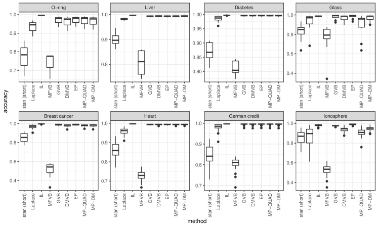
Figure 1: Boxplot of accuracies (as defined by (32)) for all marginal posterior densities and for all datasets and methods considered.

Figure 2: Scatterplot of errors in posterior means (${\mathbb{E}}_{q}(\theta_{j})-{\mathbb{E}}(\theta_{j}\,|\,{\bf y})$) on the x-axis, and errors in posterior means ($\mbox{sd}_{q}(\theta_{j})-\mbox{sd}(\theta_{j}\,|\,{\bf y})$) on the y-axis using stan (long run) as the gold standard for the Laplace, MFVB and MP methods.

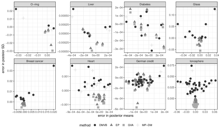
Figure 3: Scatterplot of errors in posterior means (${\mathbb{E}}_{q}(\theta_{j})-{\mathbb{E}}(\theta_{j}\,|\,{\bf y})$) on the x-axis, and errors in posterior means ($\mbox{sd}_{q}(\theta_{j})-\mbox{sd}(\theta_{j}\,|\,{\bf y})$) on the y-axis using stan (long run) as the gold standard for the DMVB, EP, GVA, and MP-DM methods.

In terms of accuracies and biases, based on Figures 1, 2 and 3, it is clear that IL, GVB, DMVB, EP, and both MP variants are all very accurate than stan (with a short run), Laplace, and MFVB. MP-DM appears to be more accurate than MP-QUAD, which is curious since MP-QUAD approximates the integral (31) more accurately. We speculate that the delta method approximation prevents overshooting the the posterior mean by underestimating (31) for high influence points. MP-DM and DMVB have similar accuracy, but are both less accurate than GVA. Finally, EP and the improved Laplace method are the most accurate. However the differences between IL, GVB, DMVB, EP, and both MP variants are small.

We will now compare timings of the different methods, but make the following caveats. An observed difference in computation times between methods may be mainly be attributed to the following reasons: (i) computational complexity; (ii) speed and stringency of convergence; and (iii) implementation language. Caveats aside, based on Table 1, the methods from fastest to slowest are Laplace, MFVB, EP (due to being implemented in C++), then DMVB and MP-DM (on some datasets one is faster and on other datasets the other), GVA-Direct, Improved Laplace, MP-QUAD, GVA-DSCB, and then rstan. We believe that MP-QUAD is slow on the datasets Glass, Cancer, and Ionosphere because trapezoidal quadrature is used due to the high number of high influence points for these datasets. Overall MP-DM represents a good trade off between speed and accuracy.

Method	Variant	O-ring	Liver	Diabetes	Glass	Cancer	Heart	German	Ionosphere
rstan	Long	35.16	334.25	391.75	679.70	1234.50	271.33	1576.09	1793.79
rstan	Short	2.33	5.89	5.62	11.59	17.43	8.71	18.36	18.62
Laplace		$*$	$*$	$*$	$*$	0.01	$*$	0.01	0.02
IL		0.10	0.45	1.05	1.06	2.52	1.40	9.06	12.02
MFVB		$*$	$*$	0.01	0.07	0.16	0.01	0.04	0.27
EP		$*$	0.01	0.01	0.01	0.03	0.02	0.16	0.18
DMVB		0.01	0.04	0.05	0.06	0.13	0.10	0.33	0.26
GVB	BFGS	0.04	0.09	0.07	2.85	1.75	0.16	0.34	11.33
GVB	DSVB	1.39	4.14	7.85	25.43	9.57	6.22	5.38	18.09
MP	QUAD	0.09	0.04	0.03	12.44	9.46	0.07	0.13	34.76
MP	DM	$*$	0.01	0.01	0.23	0.30	0.04	0.10	0.61

Table 1: Times (in seconds) for all of the methods (and variants we considered) for all datasets used. $*$ indicates less than $0.005$.

7 Conclusion

We have developed the the moment propagation method and shown that it can be used to develop algorithms that recover the true posterior distributions for all parameters of linear regression and multivariate normal models. We have developed a MP based algorithm for probit regression, shown it gives asymptotically correct posterior mean and covariance estimates, and shown that it can be effective on real data compared to a variety of other techniques. For linear and multivariate normal models we have shown that MP can use higher order posterior moments leading to more accurate posterior approximations. Lastly, it is clear that MFVB and MP updates can be interwoven without further difficulty.

Despite these contributions MP still has a number of limitations. We have only presented work here where there are two sets of components, and have only considered conjugate models. These are severe limitations, but our current work suggests that these are not insurmountable ones. We have left several theoretical avenues to explore. Convergence issues have been only dealt with at a superficial level. When does MP converge?, When are the fixed points unique? What is the rate of convergence MP methods? Can the rate of convergence be accelerated? Using Gaussian $q$-densities when are estimates asymptotically correct? When does parameterization matter and choice of approximated posterior moments matter? Can these methods be automated in a similar way to MFVB (e.g. Winn and Bishop, 2005)? All such questions remain unanswered and are subject to future work.

These appendices will appear as an online supplement.

Appendix A: Moment Results

In this appendix we summarise various moment results for the multivariate Gaussian distribution, the multivariate t-distribution, and the Inverse-Wishart distribution.

A.1 Moments for the Multivariate Gaussian Distribution

Mathai and Provost (1992) show that the $s$th cumulant of ${\bf x}^{T}{\bf A}{\bf x}$ where ${\bf A}$ is a $p\times p$ symmetric matrix and ${\bf x}\sim N_{p}({\boldsymbol{\mu}},{\boldsymbol{\Sigma}})$ is given by

$$\kappa(s)=2^{s-1}s!\left[\frac{\mbox{tr}({\bf A}{\boldsymbol{\Sigma}})^{s}}{s}+{\boldsymbol{\mu}}^{T}({\bf A}{\boldsymbol{\Sigma}})^{s-1}{\bf A}{\boldsymbol{\mu}}\right].$$

The $h$th moment of ${\bf x}^{T}{\bf A}{\bf x}$ can be calculated recursively using these cumulant via

$${\mathbb{E}}[({\bf x}^{T}{\bf A}{\bf x})^{h}]=\sum_{i=0}^{h-1}\frac{(h-1)!}{(h-1-i)!i!}\kappa(h-i){\mathbb{E}}[({\bf x}^{T}{\bf A}{\bf x})^{i}]$$

with ${\mathbb{E}}[({\bf x}^{T}{\bf A}{\bf x})^{0}]=1$.

We can use the above moments to derive

$$\begin{array}[]{rl}{\mathbb{E}}\left[({\bf x}^{T}{\bf A}{\bf x})^{2}\right]&\displaystyle=2\mbox{tr}({\bf A}{\boldsymbol{\Sigma}}{\bf A}{\boldsymbol{\Sigma}})+4{\boldsymbol{\mu}}^{T}{\bf A}{\boldsymbol{\Sigma}}{\bf A}{\boldsymbol{\mu}}+\left[{\boldsymbol{\mu}}^{T}{\bf A}{\boldsymbol{\mu}}+\mbox{tr}({\bf A}{\boldsymbol{\Sigma}})\right]^{2}\\[8.61108pt] {\mathbb{V}}({\bf x}^{T}{\bf A}{\bf x})&\displaystyle=2\operatorname{tr}({\bf A}{\boldsymbol{\Sigma}}{\bf A}{\boldsymbol{\Sigma}})+4{\boldsymbol{\mu}}^{T}{\bf A}{\boldsymbol{\Sigma}}{\bf A}{\boldsymbol{\mu}\par}\\[8.61108pt] {\mathbb{C}}({\bf x}^{T}{\bf A}{\bf x},{\bf x}^{T}{\bf B}{\bf x})&\displaystyle=2\operatorname{tr}({\bf A}{\boldsymbol{\Sigma}}{\bf B}{\boldsymbol{\Sigma}})+4{\boldsymbol{\mu}}^{T}{\bf A}{\boldsymbol{\Sigma}}{\bf B}{\boldsymbol{\mu}}.\par\par\end{array}$$ (33)

A.2 Moments for the Multivariate $t$ Distribution

The $p$-variate $t$ distribution denoted ${\bf x}\sim t_{p}({\boldsymbol{\mu}},{\boldsymbol{\Sigma}},\nu)$ with density

$$p({\bf x})=\frac{\Gamma\left[(\nu+p)/2\right]}{\Gamma(\nu/2)\nu^{p/2}\pi^{p/2}\mbox{det}({\boldsymbol{\Sigma}})^{1/2}}\left[1+\frac{1}{\nu}({\mathbf{x}}-{\boldsymbol{\mu}})^{\rm T}{\boldsymbol{\Sigma}}^{-1}({\mathbf{x}}-{\boldsymbol{\mu}})\right]^{-(\nu+p)/2}$$

where ${\boldsymbol{\mu}}$, ${\boldsymbol{\Sigma}}$ and $\nu$ are the location, scale and degrees of freedom parameters respectively. The mean and variance of ${\bf x}$ are given by ${\mathbb{E}}({\bf x})={\boldsymbol{\mu}}$ (provided $\nu>1$), covariance ${\mathbb{V}}({\bf x})=\nu{\boldsymbol{\Sigma}}/(\nu-2)$ (provided $\nu>2$).

Theorem 2.1 of Rong et al. (2012) If ${\bf x}\sim t({\boldsymbol{\mu}},a{\boldsymbol{\Sigma}},b)$ and ${\bf A}$ is a symmetric matrix then

$$\begin{array}[]{rl}{\mathbb{E}}\left[\left({\bf x}^{T}{\bf A}{\bf x}\right)^{2}\right]&\displaystyle=\frac{a^{2}b^{2}}{(b-2)(b-4)}\left[2\,\mbox{tr}({\bf A}{\boldsymbol{\Sigma}}{\bf A}{\boldsymbol{\Sigma}})+\mbox{tr}({\bf A}{\boldsymbol{\Sigma}})^{2}\right]\\[8.61108pt] &\displaystyle\qquad+\frac{4ab}{b-2}{\boldsymbol{\mu}}^{T}{\bf A}{\boldsymbol{\Sigma}}{\bf A}{\boldsymbol{\mu}}+({\boldsymbol{\mu}}^{T}{\bf A}{\boldsymbol{\mu}})^{2}+\frac{2ab}{b-2}({\boldsymbol{\mu}}^{T}{\bf A}{\boldsymbol{\mu}})\mbox{tr}({\bf A}{\boldsymbol{\Sigma}}),\end{array}$$ (34)

$${\mathbb{V}}({\bf x}^{T}{\bf A}{\bf x})=\frac{2a^{2}b^{2}\mbox{tr}({\bf A}{\boldsymbol{\Sigma}}{\bf A}{\boldsymbol{\Sigma}})}{(b-2)(b-4)}+\frac{2a^{2}b^{2}[\mbox{tr}({\bf A}{\boldsymbol{\Sigma}})]^{2}}{(b-2)^{2}(b-4)}+\frac{4ab}{b-2}{\boldsymbol{\mu}}^{T}{\bf A}{\boldsymbol{\Sigma}}{\bf A}{\boldsymbol{\mu}}.$$ (35)

and

$${\mathbb{C}}({\bf x}^{T}{\bf A}{\bf x},{\bf x}^{T}{\bf B}{\bf x})\displaystyle=\frac{2a^{2}b^{2}\,\mbox{tr}({\bf A}{\boldsymbol{\Sigma}}{\bf B}{\boldsymbol{\Sigma}})}{(b-2)(b-4)}+\frac{2a^{2}b^{2}\,\mbox{tr}({\bf A}{\boldsymbol{\Sigma}})\mbox{tr}({\bf B}{\boldsymbol{\Sigma}})}{(b-2)^{2}(b-4)}+\frac{4ab({\boldsymbol{\mu}}^{T}{\bf A}{\boldsymbol{\Sigma}}{\bf B}{\boldsymbol{\mu}})}{b-2}.$$ (36)

A.3 Moments for the Inverse-Wishart Distribution

The following are found in von Rosen (1988).

Theorem 3.1 of von Rosen (1988): Let ${\boldsymbol{\Sigma}}\sim\mbox{IW}_{p}({\boldsymbol{\Psi}},d)$ then

• $\displaystyle{\mathbb{E}}({\boldsymbol{\Sigma}})=\frac{{\boldsymbol{\Psi}}}{d-p-1}$,        if $d-p-1>0$;

Corollary 3.1 of von Rosen (1988): Let ${\boldsymbol{\Sigma}}\sim\mbox{IW}_{p}({\boldsymbol{\Psi}},d)$ with

$$\begin{array}[]{c}c_{2}^{-1}=(d-p)(d-p-1)(d-p-3),\qquad c_{1}=(d-p-2)c_{2},\\[4.30554pt] \displaystyle c_{3}=\frac{d-p-3}{(d-p-5)(d-p+1)},\qquad\mbox{and}\qquad c_{4}=\frac{2}{(d-p-5)(d+p+1)}.\end{array}$$

Then,

• if $d-p-3>0$,

  $$\begin{array}[]{rl}\displaystyle{\mathbb{E}}\left[{\boldsymbol{\Sigma}}^{2}\right]=(c_{1}+c_{2}){\boldsymbol{\Psi}}^{2}+{\color[rgb]{1,0,0}c_{2}}{\boldsymbol{\Psi}}\mbox{tr}({\boldsymbol{\Psi}});\end{array}$$

• if $d-p-5>0$,

  $$\begin{array}[]{rl}\displaystyle{\mathbb{E}}\left[{\boldsymbol{\Sigma}}^{3}\right]&\displaystyle=(c_{3}c_{1}+c_{3}c_{2}+c_{4}c_{1}+5c_{4}c_{2}){\boldsymbol{\Psi}}^{3}+(2c_{3}c_{2}+c_{4}c_{1}+c_{4}c_{2})\mbox{tr}({\boldsymbol{\Psi}}){\boldsymbol{\Psi}}^{2}\\[8.61108pt] &\displaystyle\quad-(c_{3}c_{2}+c_{4}c_{2})\mbox{tr}({\boldsymbol{\Sigma}}^{-2}){\boldsymbol{\Psi}}-c_{4}c_{2}(\mbox{tr}({\boldsymbol{\Psi}}))^{2}{\boldsymbol{\Psi}};\end{array}$$

• if $d-p-5>0$,

  $$\begin{array}[]{rl}\displaystyle{\mathbb{E}}\left[\mbox{tr}({\boldsymbol{\Sigma}}^{2}){\boldsymbol{\Sigma}}\right]&\displaystyle=c_{4}(c_{1}+c_{2}){\boldsymbol{\Psi}}^{3}+(c_{4}c_{1}+c_{3}c_{2})[\mbox{tr}({\boldsymbol{\Psi}})]^{2}{\boldsymbol{\Psi}}\\[8.61108pt] &\displaystyle\quad+(c_{3}c_{1}+c_{3}c_{2}+c_{4}c_{2})\mbox{tr}({\boldsymbol{\Psi}}^{2}){\boldsymbol{\Psi}}-2c_{4}c_{2}\mbox{tr}({\boldsymbol{\Psi}}){\boldsymbol{\Psi}}^{2};\end{array}$$

• if $d-p-5>0$,

  $$\begin{array}[]{rl}\displaystyle{\mathbb{E}}\left[\mbox{tr}({\boldsymbol{\Sigma}})^{3}\right]&\displaystyle=c_{3}c_{1}\left[\mbox{tr}({\boldsymbol{\Psi}})^{3}\right]+4c_{4}c_{2}\mbox{tr}({\boldsymbol{\Psi}}^{3})+2(c_{4}c_{1}+c_{3}c_{2})\mbox{tr}({\boldsymbol{\Psi}}^{2})\mbox{tr}({\boldsymbol{\Psi}});\end{array}$$

• if $d-p-3>0$,

  $${\mathbb{E}}\left[\mbox{tr}({\boldsymbol{\Sigma}}){\boldsymbol{\Sigma}}\right]=c_{1}\mbox{tr}({\boldsymbol{\Psi}}){\boldsymbol{\Psi}}+2c_{2}{\boldsymbol{\Psi}}^{2}$$

• if $d-p-1>0$,

  $${\mathbb{E}}\left[{\boldsymbol{\Sigma}}\otimes{\boldsymbol{\Sigma}}^{-1}\right]=\frac{d}{d-p-1}{\boldsymbol{\Psi}}\otimes{\boldsymbol{\Psi}}^{-1}-\frac{1}{d-p-1}\left[\mbox{vec}({\bf I}_{p})\mbox{vec}({\bf I}_{p})^{T}+{\bf K}_{p,p}\right];\quad\mbox{and}$$

• if $d-p-1>0$,

  $${\mathbb{E}}\left[\mbox{tr}({\boldsymbol{\Sigma}}){\boldsymbol{\Sigma}}^{-1}\right]=\frac{d}{d-p-1}\mbox{tr}({\boldsymbol{\Psi}}){\boldsymbol{\Psi}}^{-1}-\frac{2}{d-p-1}{\bf I}_{p}.$$

Note that the red highlighted $c_{2}$ coefficient in (i) above is written as $c_{1}$ in von Rosen (1988), presumably a typo. The above expression is in (i) is correct. Note that the expression for $c_{3}$ is different from the Wikipedia entry ‘Inverse-Wishart distribution’.

The variance/covariances for elements of ${\boldsymbol{\Sigma}}$ are given by (see Press, S.J. (1982) “Applied Multivariate Analysis”, 2nd ed. (Dover Publications, New York))

$$\begin{array}[]{rl}{\mathbb{V}}(\Sigma_{ij})\par&\displaystyle=\frac{(d-p+1)\psi_{ij}^{2}+(d-p-1)\psi_{ii}\psi_{jj}}{(d-p)(d-p-1)^{2}(d-p-3)},\par\\[12.91663pt] {\mathbb{V}}(\Sigma_{ii})&\displaystyle=\frac{2\psi_{ii}^{2}}{(d-p-1)^{2}(d-p-3)},\qquad\mbox{and}\par\\[12.91663pt] {\mathbb{C}}(\Sigma_{ij},\Sigma_{k\ell})&\displaystyle=\frac{2\psi_{ij}\psi_{k\ell}+(d-p-1)(\psi_{ik}\psi_{j\ell}+\psi_{i\ell}\psi_{kj})}{(d-p)(d-p-1)^{2}(d-p-3)}.\par\par\end{array}$$ (37)

Note that the element-wise variance matrix for ${\boldsymbol{\Sigma}}$ is given by

$${\mathbb{E}}{\mathbb{W}}{\mathbb{V}}({\boldsymbol{\Sigma}})=\frac{(d-p+1)({\boldsymbol{\Psi}}\circ{\boldsymbol{\Psi}})}{(d-p)(d-p-1)^{2}(d-p-3)}+\frac{(d-p-1)\mbox{dg}({\boldsymbol{\Psi}})\mbox{dg}({\boldsymbol{\Psi}})^{T}}{(d-p)(d-p-1)^{2}(d-p-3)}.$$

where $\circ$ denote the Hadamard product, i.e., if ${\bf A}$ and ${\bf B}$ are of conforming dimensions then $({\bf A}\circ{\bf B})_{ij}=a_{ij}b_{ij}$, and with diagonal elements

$$\mbox{dg}[{\mathbb{E}}{\mathbb{W}}{\mathbb{V}}({\boldsymbol{\Sigma}})]=\frac{2\mbox{dg}({\boldsymbol{\Psi}})^{2}}{(d-p-1)(d-p-3)}.$$

Appendix B: Example from Bishop (2006)

Following Bishop (2006) (Section 10.1.2) suppose that ${\boldsymbol{\theta}}\,|\,{\mathcal{D}}\sim N_{d}({\boldsymbol{\mu}},{\boldsymbol{\Sigma}})$ with ${\mathcal{D}}=\{{\boldsymbol{\mu}},{\boldsymbol{\Sigma}}\}$. Suppose that we partition ${\boldsymbol{\theta}}$ into ${\boldsymbol{\theta}}_{1}$ and ${\boldsymbol{\theta}}_{2}$ of dimensions $d_{1}$ and $d_{2}$ respectively and partition ${\boldsymbol{\mu}}$ and ${\boldsymbol{\Sigma}}$ conformably as

$${\boldsymbol{\mu}}=\left[\begin{array}[]{c}{\boldsymbol{\mu}}_{1}\\ {\boldsymbol{\mu}}_{2}\end{array}\right]\quad\mbox{and}\quad{\boldsymbol{\Sigma}}=\left[\begin{array}[]{cc}{\boldsymbol{\Sigma}}_{11}&{\boldsymbol{\Sigma}}_{12}\\ {\boldsymbol{\Sigma}}_{21}&{\boldsymbol{\Sigma}}_{22}\end{array}\right].$$

Note that the exact marginal distributions are ${\boldsymbol{\theta}}_{i}\,|\,{\mathcal{D}}\sim N_{d_{i}}({\boldsymbol{\mu}}_{i},{\boldsymbol{\Sigma}}_{ii})$ and the conditional distributions are ${\boldsymbol{\theta}}_{i}\,|\,{\mathcal{D}},{\boldsymbol{\theta}}_{-i}\sim N_{d_{i}}\left({\boldsymbol{\mu}}_{i}-{\boldsymbol{\Sigma}}_{i,-i}{\boldsymbol{\Sigma}}_{-i,-i}^{-1}({\boldsymbol{\theta}}_{-i}-{\boldsymbol{\mu}}_{-i}),{\boldsymbol{\Sigma}}_{ii}-{\boldsymbol{\Sigma}}_{i,-i}{\boldsymbol{\Sigma}}_{-i,-i}^{-1},{\boldsymbol{\Sigma}}_{-i,i}\right)$. We will now compare the MFVB and MP approximations for this toy example.

MFVB: Letting $q({\boldsymbol{\theta}})=q_{1}({\boldsymbol{\theta}}_{1})\,q_{2}({\boldsymbol{\theta}}_{2})$ and applying (3) leads to normally distributed $q$-densities $q({\boldsymbol{\theta}}_{i})=\phi({\boldsymbol{\theta}}_{i};\widetilde{{\boldsymbol{\mu}}}_{i},\widetilde{{\boldsymbol{\Sigma}}}_{i})$ (denoting a multivariate Gaussian density for ${\boldsymbol{\theta}}_{i}$ with mean $\widetilde{{\boldsymbol{\mu}}}_{i}$ and covariance $\widetilde{{\boldsymbol{\Sigma}}}_{i}$), updates

$$\widetilde{{\boldsymbol{\mu}}}_{i}\leftarrow{\boldsymbol{\mu}}_{i}-{\boldsymbol{\Sigma}}_{i,-i}{\boldsymbol{\Sigma}}_{-i,-i}^{-1}(\widetilde{{\boldsymbol{\mu}}}_{-i}-{\boldsymbol{\mu}}_{-i})\quad\mbox{and}\quad\widetilde{{\boldsymbol{\Sigma}}}_{i}\leftarrow{\boldsymbol{\Sigma}}_{ii}-{\boldsymbol{\Sigma}}_{i,-i}{\boldsymbol{\Sigma}}_{-i,-i}^{-1},{\boldsymbol{\Sigma}}_{-i,i}.$$ (38)

The consistency conditions require (38) to hold for $i\in\{1,2\}$ (with “$\leftarrow$” replaced with “$=$”). Solving these consistency equations leads to leads to a unique solution given by

$$q({\boldsymbol{\theta}}_{i})=N_{d_{i}}({\boldsymbol{\mu}}_{i},{\boldsymbol{\Sigma}}_{ii}-{\boldsymbol{\Sigma}}_{i,-i}{\boldsymbol{\Sigma}}_{-i,-i}^{-1},{\boldsymbol{\Sigma}}_{-i,i}).$$

Hence, comparing variances with the true marginal distributions we see that MFVB underestimates the posterior variance, provided ${\boldsymbol{\Sigma}}_{i,-i}\neq{\bf 0}$, i.e., there is no posterior dependence between ${\boldsymbol{\theta}}_{1}$ and ${\boldsymbol{\theta}}_{2}$.

Remark: Extrapolating to situations where the true posterior is approximately normal, e.g., where the Bernstein–von Mises theorem holds (see for example Vaart, 1998, Section 10.2), we see that factorizing $q$-densities will often lead to underestimating posterior variances. Further, in cases where there is approximately parameter orthogonality the off diagonal block of the posterior variance, analogous to ${\boldsymbol{\Sigma}}_{i,-i}$ above, will be approximately ${\bf 0}$, leading to better MFVB approximations.

MP: Suppose we model the marginal posterior distributions as $q({\boldsymbol{\theta}}_{i})=\phi({\boldsymbol{\theta}}_{i};\widetilde{{\boldsymbol{\mu}}}_{i},\widetilde{{\boldsymbol{\Sigma}}}_{i})$, $i\in\{1,2\}$. Then the MP posterior mean and covariance of ${\boldsymbol{\theta}}_{1}$ is given by

$$\begin{array}[]{rl}{\mathbb{E}}_{q}^{MP}({\boldsymbol{\theta}}_{1})&\displaystyle={\mathbb{E}}_{q}\left[{\mathbb{E}}({\boldsymbol{\theta}}_{1}\,|\,{\mathcal{D}},{\boldsymbol{\theta}}_{2})\right]={\boldsymbol{\mu}}_{1},\qquad\mbox{and}\\[8.61108pt] {\mathbb{V}}_{q}^{MP}({\boldsymbol{\theta}}_{1})&\displaystyle={\mathbb{E}}_{q}\left[{\mathbb{V}}({\boldsymbol{\theta}}_{1}\,|\,{\mathcal{D}},{\boldsymbol{\theta}}_{2})\right]+{\mathbb{V}}_{q}\left[{\mathbb{E}}({\boldsymbol{\theta}}_{1}\,|\,{\mathcal{D}},{\boldsymbol{\theta}}_{2})\right]\\[8.61108pt] &\displaystyle={\boldsymbol{\Sigma}}_{11}-{\boldsymbol{\Sigma}}_{12}{\boldsymbol{\Sigma}}_{22}^{-1},{\boldsymbol{\Sigma}}_{21}+{\boldsymbol{\Sigma}}_{12}{\boldsymbol{\Sigma}}_{22}^{-1}\widetilde{{\boldsymbol{\Sigma}}}_{2}{\boldsymbol{\Sigma}}_{22}^{-1}{\boldsymbol{\Sigma}}_{21}.\par\end{array}$$

Similarly for ${\mathbb{E}}_{q}^{MP}({\boldsymbol{\theta}}_{2})$ and ${\mathbb{V}}_{q}^{MP}({\boldsymbol{\theta}}_{2})$. Equating $q$-density and MP means and variances leads to the updates

$$\widetilde{{\boldsymbol{\mu}}}_{i}\leftarrow{\boldsymbol{\mu}}_{i}\qquad\mbox{and}\qquad\widetilde{{\boldsymbol{\Sigma}}}_{i}\leftarrow{\boldsymbol{\Sigma}}_{ii}+{\boldsymbol{\Sigma}}_{i,-i}{\boldsymbol{\Sigma}}_{-i,-i}^{-1}(\widetilde{{\boldsymbol{\Sigma}}}_{-i}-{\boldsymbol{\Sigma}}_{-i,-i}^{-1}){\boldsymbol{\Sigma}}_{-i,-i}^{-1}{\boldsymbol{\Sigma}}_{-i,i}$$

for $i\in\{1,2\}$. Since the means are fixed, the consistency conditions for the approximate posterior variances $\widetilde{{\boldsymbol{\Sigma}}}_{i}$’s need to simultaneously satisfy

$$\begin{array}[]{rl}\widetilde{{\boldsymbol{\Sigma}}}_{1}&\displaystyle={\boldsymbol{\Sigma}}_{11}+{\boldsymbol{\Sigma}}_{12}{\boldsymbol{\Sigma}}_{22}^{-1}(\widetilde{{\boldsymbol{\Sigma}}}_{2}-{\boldsymbol{\Sigma}}_{22}){\boldsymbol{\Sigma}}_{22}^{-1}{\boldsymbol{\Sigma}}_{21},\qquad\mbox{and}\\[4.30554pt] \widetilde{{\boldsymbol{\Sigma}}}_{2}&\displaystyle={\boldsymbol{\Sigma}}_{22}+{\boldsymbol{\Sigma}}_{21}{\boldsymbol{\Sigma}}_{11}^{-1}(\widetilde{{\boldsymbol{\Sigma}}}_{1}-{\boldsymbol{\Sigma}}_{11}){\boldsymbol{\Sigma}}_{11}^{-1}{\boldsymbol{\Sigma}}_{12}.\par\end{array}$$

Substituting the second above equation into the first and rearranging leads to

$$(\widetilde{{\boldsymbol{\Sigma}}}_{1}-{\boldsymbol{\Sigma}}_{11})-({\boldsymbol{\Sigma}}_{12}{\boldsymbol{\Sigma}}_{22}^{-1}{\boldsymbol{\Sigma}}_{21}){\boldsymbol{\Sigma}}_{11}^{-1}(\widetilde{{\boldsymbol{\Sigma}}}_{1}-{\boldsymbol{\Sigma}}_{11}){\boldsymbol{\Sigma}}_{11}^{-1}({\boldsymbol{\Sigma}}_{12}{\boldsymbol{\Sigma}}_{22}^{-1}{\boldsymbol{\Sigma}}_{21})={\bf 0}$$

which we can write as

$$[{\boldsymbol{\Sigma}}_{11}-{\boldsymbol{\Sigma}}_{12}{\boldsymbol{\Sigma}}_{22}^{-1}{\boldsymbol{\Sigma}}_{21}]{\boldsymbol{\Sigma}}_{11}^{-1}(\widetilde{{\boldsymbol{\Sigma}}}_{1}-{\boldsymbol{\Sigma}}_{11}){\boldsymbol{\Sigma}}_{11}^{-1}[{\boldsymbol{\Sigma}}_{11}+{\boldsymbol{\Sigma}}_{12}{\boldsymbol{\Sigma}}_{22}^{-1}{\boldsymbol{\Sigma}}_{21}]={\bf 0}.$$

The left-hand side square bracketed term is the Schur’s complement of a positive definite matrix, and hence convertible (see Horn and Johnson, 2012, Theorem 7.7.7). It then follows, using basic properties of positive definite matrices that $\widetilde{{\boldsymbol{\Sigma}}}_{1}={\boldsymbol{\Sigma}}_{11}$ and $\widetilde{{\boldsymbol{\Sigma}}}_{2}={\boldsymbol{\Sigma}}_{22}$. Hence, the MP method leads to the exact marginal posterior distributions.

Remark: Note that the $\mbox{cov}({\boldsymbol{\theta}}_{1},{\boldsymbol{\theta}}_{2}\,|\,{\mathcal{D}})$ does not need to be calculated implicitly or stored unlike FFVB where ${\boldsymbol{\theta}}_{1}$ and ${\boldsymbol{\theta}}_{2}$ are modelled jointly. Note that for this problem MFVB iterations update the means while the variances remain fixed, where as for the MP approximations, the means remain fixed across iterations and the covariances are updated.

Appendix C: Derivations for linear models

In this appendix we provide detailed derivations for all of the material in Section 4.

C.1 Exact posterior distributions

The full conditional distributions are given by

$$\begin{array}[]{rl}{\boldsymbol{\beta}}\,|\,{\bf y},\sigma^{2}&\displaystyle\sim N_{p}\left(\frac{g}{1+g}\widehat{{\boldsymbol{\beta}}},\frac{g}{1+g}\sigma^{2}({\bf X}^{T}{\bf X})^{-1}\right),\qquad\mbox{and}\par\\[8.61108pt] \sigma^{2}\,|\,{\bf y},{\boldsymbol{\beta}}&\displaystyle\sim\mbox{IG}\left(A+\tfrac{1}{2}(n+p),B({\boldsymbol{\beta}})\right),\par\\[8.61108pt] \mbox{where}\qquad B({\boldsymbol{\beta}})&\displaystyle\equiv B+\tfrac{1}{2}\|{\bf y}-{\bf X}{\boldsymbol{\beta}}\|^{2}+\tfrac{1}{2g}{\boldsymbol{\beta}}^{T}{\bf X}^{T}{\bf X}{\boldsymbol{\beta}}.\end{array}$$ (39)

The exact posterior distributions for ${\boldsymbol{\beta}}$ and $\sigma^{2}$ are given by

$$\begin{array}[]{rl}{\boldsymbol{\beta}}\,|\,{\bf y}&\displaystyle\sim t\left(u\widehat{{\boldsymbol{\beta}}},\left(\frac{B+\frac{n}{2}\widehat{\sigma}_{u}^{2}}{A+\tfrac{n}{2}}\right)u({\bf X}^{T}{\bf X})^{-1},2A+n\right),\qquad\mbox{and}\par\\[8.61108pt] \sigma^{2}\,|\,{\bf y}&\displaystyle\sim\mbox{IG}\left(A+\frac{n}{2},B+\frac{n\widehat{\sigma}_{u}^{2}}{2}\right),\end{array}$$ (40)

where

$$\begin{array}[]{c}\displaystyle\widehat{{\boldsymbol{\beta}}}=({\bf X}^{T}{\bf X})^{-1}{\bf X}^{T}{\bf y},\quad u=\frac{g}{1+g}\quad\mbox{and}\quad\widehat{\sigma}_{u}^{2}=\frac{1}{n}[\,\|{\bf y}\|^{2}-u\,{\bf y}^{T}{\bf X}({\bf X}^{T}{\bf X})^{-1}{\bf X}^{T}{\bf y}\,].\end{array}$$ (41)

Note that as $g\to\infty$, $\sigma_{u}^{2}$ converges to the maximum likelihood estimator for $\sigma^{2}$.

C.2 Derivations for MFVB

For the linear model described in Section 4 with $q$-density factorization $q({\boldsymbol{\mu}},\sigma^{2})=q({\boldsymbol{\mu}},\sigma^{2})$, the updates for $q({\boldsymbol{\mu}})$ and $q(\sigma^{2})$ are derived via

$$\begin{array}[]{rl}q({\boldsymbol{\beta}})&\displaystyle\propto\exp\left[{\mathbb{E}}_{q(\sigma^{2})}\left\{-\tfrac{1}{2\sigma^{2}}\|{\bf y}-{\bf X}{\boldsymbol{\beta}}\|^{2}-\tfrac{1}{2g\sigma^{2}}{\bf X}^{T}{\bf X}\right\}\right]\par\\[8.61108pt] &\displaystyle\propto\exp\left[{\mathbb{E}}_{q(\sigma^{2})}\left\{\tfrac{{\bf y}^{T}{\bf X}{\boldsymbol{\beta}}}{2\sigma^{2}}-\tfrac{1+1/g}{2\sigma^{2}}{\boldsymbol{\mu}}^{T}{\bf X}^{T}{\bf X}{\boldsymbol{\mu}}\right\}\right]\par\par\\[8.61108pt] &\displaystyle=N_{p}\left(\widetilde{{\boldsymbol{\mu}}}\equiv u\widehat{{\boldsymbol{\beta}}},\widetilde{{\boldsymbol{\Sigma}}}\equiv u(\widetilde{B}/\widetilde{A})({\bf X}^{T}{\bf X})^{-1}\right)\quad\mbox{and}\par\\[8.61108pt] q(\sigma^{2})&\displaystyle\propto\exp\Big{[}-\left(A+\tfrac{n+p}{2}+1\right)\log(\sigma^{2})\\ &\displaystyle\qquad-{\mathbb{E}}_{q({\boldsymbol{\beta}})}\left\{B+\tfrac{1}{2}\|{\bf y}-{\bf X}\widetilde{{\boldsymbol{\mu}}}\|^{2}+\tfrac{1}{2g}\widetilde{{\boldsymbol{\mu}}}^{T}{\bf X}^{T}{\bf X}\widetilde{{\boldsymbol{\mu}}}+\tfrac{1}{2u}\mbox{tr}\left({\bf X}^{T}{\bf X}\widetilde{{\boldsymbol{\Sigma}}}\right)\right\}\sigma^{-2}\par\par\Big{]}\par\\[8.61108pt] &\displaystyle=\mbox{IG}\left(\widetilde{A}\equiv A+\tfrac{n+p}{2},\widetilde{B}\equiv B+\tfrac{1}{2}\|{\bf y}-{\bf X}\widetilde{{\boldsymbol{\mu}}}\|^{2}+\tfrac{1}{2g}\widetilde{{\boldsymbol{\mu}}}^{T}{\bf X}^{T}{\bf X}\widetilde{{\boldsymbol{\mu}}}+\tfrac{1}{2u}\mbox{tr}\left({\bf X}^{T}{\bf X}\widetilde{{\boldsymbol{\Sigma}}}\right)\right).\end{array}$$

where $u=g/(1+g)$ (and noting $1+1/g=1/u$).

C.3 MFVB for linear models

The MFVB approximation for the linear model corresponding to the factorization $q({\boldsymbol{\mu}},{\boldsymbol{\Sigma}})=q({\boldsymbol{\mu}})q({\boldsymbol{\Sigma}})$ (derived in Appendix B) have $q$-densities of the forms:

$$\begin{array}[]{c}\displaystyle q({\boldsymbol{\beta}})=N_{p}(\widetilde{{\boldsymbol{\mu}}},\widetilde{{\boldsymbol{\Sigma}}})\qquad\mbox{and}\qquad q(\sigma^{2})=\mbox{IG}(\widetilde{A},\widetilde{B}),\end{array}$$

where the updates are given by equations (42) and (43) in Algorithm 7 which summarises the MFVB method for the linear model.

Note that the distributional form for $q({\boldsymbol{\beta}})$ comes directly from (3), while the true posterior follows a $t$-distribution. Hence, for any factorized $q$-density MFVB cannot be exact for this model.

Algorithm 7 MFVB for the linear model

0:  ${\bf y}\in{\mathbb{R}}^{n}$, ${\bf X}\in{\mathbb{R}}^{n\times p}$, $g>0$, $A>0$, and $B>0$.

1:  Calculate algorithm constants via (41).

2:  Initialize variational parameter $\widetilde{A}=A+\tfrac{1}{2}(n+p)$ and $\widetilde{B}=B+\tfrac{1}{2}\|{\bf y}\|^{2}$

3:  repeat

4:     Update $q({\boldsymbol{\beta}})$ parameters:

$$\widetilde{{\boldsymbol{\mu}}}\leftarrow u\widehat{{\boldsymbol{\beta}}};\qquad\displaystyle\widetilde{{\boldsymbol{\Sigma}}}\leftarrow\frac{\widetilde{B}}{\widetilde{A}}\,u({\bf X}^{T}{\bf X})^{-1}$$ (42)

5:     Update $q(\sigma^{2})$ parameters:

$$\begin{array}[]{rl}\displaystyle\widetilde{A}\displaystyle\leftarrow A+\frac{n+p}{2};\qquad\displaystyle\widetilde{B}\displaystyle\leftarrow B+\frac{\|{\bf y}-{\bf X}\widetilde{{\boldsymbol{\mu}}}\|^{2}}{2}+\frac{\widetilde{{\boldsymbol{\mu}}}^{T}{\bf X}^{T}{\bf X}\widetilde{{\boldsymbol{\mu}}}}{2g}+\frac{\mbox{tr}({\bf X}^{T}{\bf X}\widetilde{{\boldsymbol{\Sigma}}})}{2u}\end{array}$$ (43)

6:  until convergence criterion is satisfied.

To quantify MFVB’s underestimation of the marginal posterior variance, we provide the following result.

C.4 Result 2

Result 2

Let $\widetilde{{\boldsymbol{\mu}}}^{*}$, $\widetilde{{\boldsymbol{\Sigma}}}^{*}$, $\widetilde{A}^{*}$, and $\widetilde{B}^{*}$ denote the parameters of the MFVB approximate posterior upon convergence of Algorithm 7. Then, we have

$$q^{*}({\boldsymbol{\beta}})=N_{p}(\widetilde{{\boldsymbol{\mu}}}^{*},\widetilde{{\boldsymbol{\Sigma}}}^{*})\qquad\mbox{and}\qquad q^{*}(\sigma^{2})=\mbox{IG}(\widetilde{A}^{*},\widetilde{B}^{*})$$

where $\widetilde{{\boldsymbol{\mu}}}^{*}\equiv u\widehat{{\boldsymbol{\beta}}}$, $\widetilde{A}^{*}\equiv A+\frac{n+p}{2}$,

$$\begin{array}[]{c}\displaystyle\widetilde{{\boldsymbol{\Sigma}}}^{*}\equiv\left(\frac{B+\frac{n\widehat{\sigma}_{u}^{2}}{2}}{A+\frac{n}{2}}\right)u({\bf X}^{T}{\bf X})^{-1},\qquad\mbox{and}\qquad\widetilde{B}^{*}\equiv\left(\frac{A+\frac{n+p}{2}}{A+\frac{n}{2}}\right)\left(B+\frac{n\widehat{\sigma}_{u}^{2}}{2}\right).\end{array}$$

The MFVB approximation of the posterior expectation of ${\boldsymbol{\beta}}$ is exact, whereas the MFVB approximation of the posterior expectation of $\sigma^{2}$ is underestimated. The MFVB approximation of the posterior variance of ${\boldsymbol{\beta}}$ is underestimated, whereas the MFVB approximations of the posterior variance of $\sigma^{2}$ is underestimated provided $2A+n+p>4$. The MFVB approximations of the first two posterior moments for both ${\boldsymbol{\beta}}$ and $\sigma^{2}$ approaches their exact values as $n\to\infty$ (with $p$ fixed).

Let $\widetilde{{\boldsymbol{\mu}}}^{*}$, $\widetilde{{\boldsymbol{\Sigma}}}^{*}$, $\widetilde{A}^{*}$, and $\widetilde{B}^{*}$ denote the values of $\widetilde{{\boldsymbol{\mu}}}$, $\widetilde{{\boldsymbol{\Sigma}}}$, $\widetilde{A}$, and $\widetilde{B}$ at the convergence of Algorithm 7. Then the consistency equations are equivalent to the following four equations

$$\begin{array}[]{rl}\widetilde{{\boldsymbol{\mu}}}^{*}&\displaystyle=u\widehat{{\boldsymbol{\beta}}},\par\\[8.61108pt] \widetilde{{\boldsymbol{\Sigma}}}^{*}&\displaystyle=u(\widetilde{B}^{*}/\widetilde{A}^{*})({\bf X}^{T}{\bf X})^{-1},\par\\[8.61108pt] \widetilde{A}^{*}&\displaystyle=A+\tfrac{n+p}{2}\qquad\mbox{and}\par\\[8.61108pt] \widetilde{B}^{*}&\displaystyle=B+\tfrac{1}{2}\|{\bf y}-{\bf X}\widetilde{{\boldsymbol{\mu}}}^{*}\|^{2}+\tfrac{1}{2g}\widetilde{{\boldsymbol{\mu}}}_{*}^{T}{\bf X}^{T}{\bf X}\widetilde{{\boldsymbol{\mu}}}_{*}+\tfrac{u}{2}\mbox{tr}\left({\bf X}^{T}{\bf X}\widetilde{{\boldsymbol{\Sigma}}}^{*}\right).\par\end{array}$$

Substituting the expressions for $\widetilde{{\boldsymbol{\mu}}}^{*}$, $\widetilde{{\boldsymbol{\Sigma}}}^{*}$ and $\widetilde{A}_{*}$ into $\widetilde{B}_{*}$ we obtain

$$\begin{array}[]{rl}\widetilde{B}^{*}&\displaystyle=B+\frac{1}{2}\left(\|{\bf y}\|^{2}-u{\bf y}^{T}{\bf X}({\bf X}^{T}{\bf X})^{-1}{\bf X}^{T}{\bf y}\right)+\frac{p\widetilde{B}^{*}}{2A+n+p}.\par\end{array}$$

Solving for $\widetilde{B}^{*}$ we obtain

$$\widetilde{B}^{*}=\frac{A+\frac{n+p}{2}}{A+\frac{n}{2}}\left(B+\frac{n\widehat{\sigma}_{u}^{2}}{2}\right)\quad\mbox{and so}\quad\widetilde{{\boldsymbol{\Sigma}}}^{*}=u\left(\frac{B+\frac{n\widehat{\sigma}_{u}^{2}}{2}}{A+\frac{n}{2}}\right)({\bf X}^{T}{\bf X})^{-1}.$$

Hence,

$$\begin{array}[]{rl}q^{*}({\boldsymbol{\beta}})&\displaystyle\sim N\left(\widetilde{{\boldsymbol{\mu}}}^{*}\equiv u\widehat{{\boldsymbol{\beta}}},\,\widetilde{{\boldsymbol{\Sigma}}}_{*}\equiv u\left(\frac{B+\frac{n\widehat{\sigma}_{u}^{2}}{2}}{A+\frac{n}{2}}\right)({\bf X}^{T}{\bf X})^{-1}\right)\qquad\mbox{and}\par\\[17.22217pt] q^{*}(\sigma^{2})&\displaystyle\sim\mbox{IG}\left(\widetilde{A}\equiv A+\frac{n+p}{2},\widetilde{B}_{*}\equiv\frac{A+\frac{n+p}{2}}{A+\frac{n}{2}}\left(B+\frac{n\widehat{\sigma}_{u}^{2}}{2}\right)\right).\end{array}$$

Let, ${\mathbb{E}}_{q}^{VB*}({\boldsymbol{\beta}})$, ${\mathbb{V}}_{q}^{VB*}({\boldsymbol{\beta}})$, ${\mathbb{E}}_{q}^{VB*}(\sigma^{2})$ and ${\mathbb{V}}_{q}^{VB*}(\sigma^{2})$ denote the MFVB approximate means and variances of ${\boldsymbol{\beta}}$ and $\sigma^{2}$ at convergence of Algorithm 7. Then

$$\begin{array}[]{rl}{\mathbb{E}}_{q}^{VB*}({\boldsymbol{\beta}})&\displaystyle=u\widehat{{\boldsymbol{\beta}}},\par\\[8.61108pt] {\mathbb{V}}_{q}^{VB*}({\boldsymbol{\beta}})&\displaystyle=\left(\frac{B+\frac{n\widehat{\sigma}_{u}^{2}}{2}}{A+\frac{n}{2}}\right)u({\bf X}^{T}{\bf X})^{-1},\par\\[8.61108pt] {\mathbb{E}}_{q}^{VB*}(\sigma^{2})&\displaystyle=\left(\frac{A+\frac{n+p}{2}}{A+\tfrac{n+p}{2}-1}\right)\left(\frac{B+\frac{n\widehat{\sigma}_{u}^{2}}{2}}{A+\frac{n}{2}}\right)\qquad\mbox{and}\par\par\par\\[8.61108pt] {\mathbb{V}}_{q}^{VB*}(\sigma^{2})&\displaystyle=\par\par\par\frac{1}{(A+\tfrac{n+p}{2}-1)^{2}(A+\tfrac{n+p}{2}-2)}\left(\frac{A+\frac{n+p}{2}}{A+\frac{n}{2}}\right)^{2}\left(B+\frac{n\widehat{\sigma}_{u}^{2}}{2}\right)^{2}.\par\end{array}$$

The VB approximation of the posterior expectation of ${\boldsymbol{\beta}}$ is exact since ${\mathbb{E}}_{q}^{VB*}({\boldsymbol{\beta}})={\mathbb{E}}({\boldsymbol{\beta}}\,|\,{\bf y})$. Let ${\mathbb{V}}_{q}^{VB*}({\boldsymbol{\beta}})=v_{\beta}{\mathbb{V}}({\boldsymbol{\beta}}\,|\,{\bf y})$, ${\mathbb{E}}_{q}^{VB*}(\sigma^{2})=e_{\sigma}{\mathbb{E}}(\sigma^{2}\,|\,{\bf y})$, and ${\mathbb{V}}_{q}^{VB*}(\sigma^{2})=v_{\sigma}{\mathbb{V}}(\sigma^{2}\,|\,{\bf y})$, where $v_{\beta}$, $e_{\sigma}$, and $v_{\sigma}$ are given by:

$$\begin{array}[]{rl}\displaystyle v_{\boldsymbol{\beta}}&\displaystyle=\frac{A+\frac{n}{2}-1}{A+\frac{n}{2}}=1-\frac{1}{A+n/2}\\[8.61108pt] \displaystyle e_{\sigma}&\displaystyle=\left(\frac{A+\frac{n+p}{2}}{A+\tfrac{n+p}{2}-1}\right)\left(\frac{A+\frac{n}{2}-1}{A+\frac{n}{2}}\right)=1-\frac{p}{\left(2A+n\right)\left(A+(n+p)/2-1\right)}\par\\[8.61108pt] v_{\sigma}&\displaystyle=\frac{(A+\tfrac{n}{2}-2)}{(A+\tfrac{n+p}{2}-2)}\frac{(A+\frac{n+p}{2})^{2}}{(A+\tfrac{n+p}{2}-1)^{2}}\frac{(A+\frac{n}{2}-1)^{2}}{(A+\frac{n}{2})^{2}}=\left(1-\frac{p}{2A+n+p-4}\right)e_{\sigma}^{2}.\par\end{array}$$

where it is clear that $v_{\boldsymbol{\beta}}$, $e_{\sigma}$ and $v_{\sigma}$ are all less than 1 since $A$, $p>0$, and $2A+n+p>4$, and approach 1 as $n\to\infty$.

C.5 Derivations for MP - Approach 1

We will consider moment propagation approximation where $q({\boldsymbol{\beta}})=N(\widetilde{{\boldsymbol{\mu}}},\widetilde{{\boldsymbol{\Sigma}}})$ and $q(\sigma^{2})=\mbox{IG}(\widetilde{A},\widetilde{B})$. These are precisely the same distributional forms as MFVB. However, the updates for the $q$-density parameters will be different. For the update of $q({\boldsymbol{\beta}})$ using the fact that ${\boldsymbol{\beta}}\,|\,{\bf y},{\boldsymbol{\sigma}}^{2}\sim N(u\widehat{{\boldsymbol{\beta}}},\sigma^{2}u({\bf X}^{T}{\bf X})^{-1})$ we equate

$$\begin{array}[]{rll}\displaystyle{\mathbb{E}}_{q}^{MP}({\boldsymbol{\beta}})&\displaystyle={\mathbb{E}}_{q}[{\mathbb{E}}({\boldsymbol{\beta}}\,|\,{\bf y},\sigma^{2})]&\displaystyle=u\widehat{{\boldsymbol{\beta}}}\\[8.61108pt] \displaystyle{\mathbb{V}}_{q}^{MP}({\boldsymbol{\beta}})&\displaystyle={\mathbb{E}}_{q}[{\mathbb{V}}({\boldsymbol{\beta}}\,|\,{\bf y},\sigma^{2})]+{\mathbb{V}}_{q}[{\mathbb{E}}({\boldsymbol{\beta}}\,|\,{\bf y},\sigma^{2})]&\displaystyle=\frac{\widetilde{B}}{\widetilde{A}-1}u({\bf X}^{T}{\bf X})^{-1}\end{array}$$

with ${\mathbb{E}}_{q}({\boldsymbol{\beta}})=\widetilde{{\boldsymbol{\mu}}}$, and ${\mathbb{V}}_{q}({\boldsymbol{\beta}})=\widetilde{{\boldsymbol{\Sigma}}}$. Hence, using the matching (8) and solving for $\widetilde{{\boldsymbol{\mu}}}$ and $\widetilde{{\boldsymbol{\Sigma}}}$ leads to the update

$$\widetilde{{\boldsymbol{\mu}}}\leftarrow u\widehat{{\boldsymbol{\beta}}}\quad\mbox{and}\quad\widetilde{{\boldsymbol{\Sigma}}}\leftarrow\frac{\widetilde{B}}{\widetilde{A}-1}u({\bf X}^{T}{\bf X})^{-1}.$$

Similarly, for the update of $q(\sigma^{2})$ since $\sigma^{2}\,|\,{\bf y},{\boldsymbol{\beta}}\sim\mbox{IG}(A+\tfrac{1}{2}(n+p),B({\boldsymbol{\beta}}))$ we have

$$\begin{array}[]{rl}\displaystyle{\mathbb{E}}_{q}^{MP}(\sigma^{2})&\displaystyle={\mathbb{E}}_{q}[{\mathbb{E}}(\sigma^{2}\,|\,{\bf y},{\boldsymbol{\beta}})]=\frac{{\mathbb{E}}_{q}[B({\boldsymbol{\beta}})]}{A+\tfrac{n+p}{2}-1}.\\[12.91663pt] \displaystyle{\mathbb{V}}_{q}^{MP}(\sigma^{2})&\displaystyle={\mathbb{E}}_{q}[{\mathbb{V}}(\sigma^{2}\,|\,{\bf y},{\boldsymbol{\beta}})]+{\mathbb{V}}_{q}[{\mathbb{E}}(\sigma^{2}\,|\,{\bf y},{\boldsymbol{\beta}})\\[8.61108pt] &\displaystyle={\mathbb{E}}_{q}\left[\frac{B({\boldsymbol{\beta}})^{2}}{(A+\tfrac{n+p}{2}-1)^{2}(A+\tfrac{n+p}{2}-2)}\right]+{\mathbb{V}}_{q}\left[\frac{B({\boldsymbol{\beta}})}{A+\tfrac{n+p}{2}-1}\right]\\[8.61108pt] &\displaystyle=\frac{{\mathbb{E}}_{q}\left[B({\boldsymbol{\beta}})\right]^{2}}{(A+\tfrac{n+p}{2}-1)^{2}(A+\tfrac{n+p}{2}-2)}\\[8.61108pt] &\displaystyle\qquad+\left[\frac{1}{(A+\tfrac{n+p}{2}-1)^{2}(A+\tfrac{n+p}{2}-2)}+\frac{1}{(A+\tfrac{n+p}{2}-1)^{2}}\right]{\mathbb{V}}_{q}\left[B({\boldsymbol{\beta}})\right]\par\\[8.61108pt] &\displaystyle=\frac{{\mathbb{E}}_{q}\left[B({\boldsymbol{\beta}})\right]^{2}}{(A+\tfrac{n+p}{2}-1)^{2}(A+\tfrac{n+p}{2}-2)}+\frac{{\mathbb{V}}_{q}\left[B({\boldsymbol{\beta}})\right]}{(A+\tfrac{n+p}{2}-1)(A+\tfrac{n+p}{2}-2)}.\par\end{array}$$

Next,

$$\begin{array}[]{rl}{\mathbb{E}}_{q}[B({\boldsymbol{\beta}})]&\displaystyle=B+\frac{1}{2}\|{\bf y}-{\bf X}\widetilde{{\boldsymbol{\mu}}}\|^{2}+\frac{\widetilde{{\boldsymbol{\mu}}}^{T}{\bf X}^{T}{\bf X}\widetilde{{\boldsymbol{\mu}}}}{2g}+\frac{\mbox{tr}({\bf X}^{T}{\bf X}\widetilde{{\boldsymbol{\Sigma}}})}{2u}\\[8.61108pt] {\mathbb{V}}_{q}[B({\boldsymbol{\beta}})]\par&\displaystyle={\mathbb{V}}_{q}\left[B+\frac{1}{2}\|{\bf y}-{\bf X}{\boldsymbol{\beta}}\|^{2}+\frac{{\boldsymbol{\beta}}^{T}{\bf X}^{T}{\bf X}{\boldsymbol{\beta}}}{2g}\right]\\[8.61108pt] &\displaystyle={\mathbb{V}}_{q}\left[\tfrac{1}{2}{\boldsymbol{\beta}}^{T}(u^{-1}{\bf X}^{T}{\bf X}){\boldsymbol{\beta}}-{\bf y}^{T}{\bf X}{\boldsymbol{\beta}}\right]\\[8.61108pt] &\displaystyle=\frac{1}{4u^{2}}{\mathbb{V}}_{q}\left[({\boldsymbol{\beta}}-u\widehat{{\boldsymbol{\beta}}})^{T}({\bf X}^{T}{\bf X})({\boldsymbol{\beta}}-u\widehat{{\boldsymbol{\beta}}})\right]\\[8.61108pt] &\displaystyle=\frac{\operatorname{tr}[({\bf X}^{T}{\bf X}\widetilde{{\boldsymbol{\Sigma}}})^{2}]}{2u^{2}}.\end{array}$$

In the working for ${\mathbb{V}}_{q}[B({\boldsymbol{\beta}})]$ above, the first line absorbs constants into the variance operator, the second line completes the square for ${\boldsymbol{\beta}}$, the third line takes constant outside the variance operator, and the last line follows from the variance formula of for quadratic forms of multivariate normal variables, i.e., equation (33).

Hence, using the matching (9) we obtain the following equations

$${\mathbb{E}}_{q}^{MP}(\sigma^{2})=\frac{\widetilde{B}}{\widetilde{A}-1}={\mathbb{E}}_{q}(\sigma^{2})\qquad\mbox{and}\qquad{\mathbb{V}}_{q}^{MP}(\sigma^{2})=\frac{\widetilde{B}^{2}}{(\widetilde{A}-1)^{2}(\widetilde{A}-2)}={\mathbb{V}}_{q}(\sigma^{2})$$

Solving for $\widetilde{A}$ and $\widetilde{B}$ leads to the update

$$\widetilde{A}\leftarrow\frac{[{\mathbb{E}}_{q}^{MP}(\sigma^{2})]^{2}}{{\mathbb{V}}_{q}^{MP}(\sigma^{2})}+2;\qquad\displaystyle\widetilde{B}\leftarrow(\widetilde{A}-1)\,{\mathbb{E}}_{q}^{MP}(\sigma^{2}).$$ (44)

The MP approximation can them be summarized via Algorithm 3.

Result 3

Let ${\mathbb{E}}_{q}^{MP*}(\sigma^{2})$ and ${\mathbb{V}}_{q}^{MP*}(\sigma^{2})$ denote the MP approximate posterior mean and variance of $\sigma^{2}$ upon convergence of Algorithm 3. The fixed point of the moment conditions (10)–(16) lead to

$$\begin{array}[]{rl}{\mathbb{E}}_{q}^{MP*}(\sigma^{2})&\displaystyle\equiv\frac{B+\tfrac{n\widehat{\sigma}_{u}^{2}}{2}}{A+\tfrac{n}{2}-1}\quad\mbox{and}\\ {\mathbb{V}}_{q}^{MP*}(\sigma^{2})&\displaystyle\equiv\frac{1}{A+\tfrac{n+p}{2}-2}\left(1+\frac{p/2}{A+\tfrac{n+p}{2}-1}\right)\left(\frac{B+\frac{n\widehat{\sigma}_{u}^{2}}{2}}{A+\tfrac{n}{2}-1}\right)^{2}.\end{array}$$

The MP approximation of the posterior expectation of ${\boldsymbol{\beta}}$ and $\sigma^{2}$ are exact, as is the posterior variance for ${\boldsymbol{\beta}}$. Provided $n\geq 2$ the posterior variance of $\sigma^{2}$ is underestimated, but approaches its exact value as $n\to\infty$ (with $p$ fixed).

Algorithm 3 converges when the left hand side of assignments ($\leftarrow$) are equal to the right hand of assignments (at least closely). This is equivalent to the following system of equations:

$$\widetilde{{\boldsymbol{\mu}}} \displaystyle=u\widehat{{\boldsymbol{\beta}}}$$ (45)

$$\widetilde{{\boldsymbol{\Sigma}}} \displaystyle=\frac{\widetilde{B}}{\widetilde{A}-1}u({\bf X}^{T}{\bf X})^{-1}$$ (46)

$${\mathbb{E}}_{q}[B({\boldsymbol{\beta}})] \displaystyle=B+\tfrac{1}{2}\|{\bf y}-{\bf X}\widetilde{{\boldsymbol{\mu}}}\|^{2}+\tfrac{1}{2g}\widetilde{{\boldsymbol{\mu}}}^{T}{\bf X}^{T}{\bf X}\widetilde{{\boldsymbol{\mu}}}+\tfrac{1}{2u}\mbox{tr}({\bf X}^{T}{\bf X}\widetilde{{\boldsymbol{\Sigma}}})$$ (47)

$${\mathbb{V}}_{q}[B({\boldsymbol{\beta}})] \displaystyle=\frac{1}{2u^{2}}\operatorname{tr}\left[({\bf X}^{T}{\bf X}\widetilde{{\boldsymbol{\Sigma}}})^{2}\right]$$ (48)

$${\mathbb{E}}_{q}^{MP}(\sigma^{2}) \displaystyle=\frac{{\mathbb{E}}_{q}[B({\boldsymbol{\beta}})]}{A+\tfrac{n+p}{2}-1}$$ (49)

$${\mathbb{V}}_{q}^{MP}(\sigma^{2}) \displaystyle=\frac{{\mathbb{E}}_{q}[B({\boldsymbol{\beta}})]^{2}}{(A+\tfrac{n+p}{2}-1)^{2}(A+\tfrac{n+p}{2}-2)}+\frac{{\mathbb{V}}_{q}[B({\boldsymbol{\beta}})]}{(A+\tfrac{n+p}{2}-1)(A+\tfrac{n+p}{2}-2)}$$ (50)

$$\widetilde{A} \displaystyle=\frac{[{\mathbb{E}}_{q}^{MP}(\sigma^{2})]^{2}}{{\mathbb{V}}_{q}^{MP}(\sigma^{2})}+2$$ (51)

$$\displaystyle\widetilde{B} \displaystyle=(\widetilde{A}-1){\mathbb{E}}_{q}^{MP}(\sigma^{2})$$ (52)

Substituting $\widetilde{{\boldsymbol{\mu}}}$ and $\widetilde{{\boldsymbol{\Sigma}}}$ into the expressions for ${\mathbb{E}}_{q}[B({\boldsymbol{\beta}})]$ and ${\mathbb{V}}_{q}[B({\boldsymbol{\beta}})]$, we obtain

$$\begin{array}[]{rl}{\mathbb{E}}_{q}[B({\boldsymbol{\beta}})]&\displaystyle=B+\tfrac{1}{2}n\widehat{\sigma}_{u}^{2}+\tfrac{1}{2}p\,{\mathbb{E}}_{q}^{MP}(\sigma^{2})\\[8.61108pt] {\mathbb{V}}_{q}[B({\boldsymbol{\beta}})]&\displaystyle=\tfrac{1}{2}p\,[{\mathbb{E}}_{q}^{MP}(\sigma^{2})]^{2}.\end{array}$$

which follows from the facts that

$$\begin{array}[]{rl}\displaystyle\|{\bf y}-{\bf X}\widetilde{{\boldsymbol{\mu}}}\|^{2}+g^{-1}\widetilde{{\boldsymbol{\mu}}}^{T}{\bf X}^{T}{\bf X}\widetilde{{\boldsymbol{\mu}}}&\displaystyle=n\widehat{\sigma}_{u}^{2}\\[8.61108pt] u^{-1}\operatorname{tr}\left[({\bf X}^{T}{\bf X}\widetilde{{\boldsymbol{\Sigma}}})\right]&\displaystyle=\left(\frac{\widetilde{B}}{\widetilde{A}-1}\right)p=p\,{\mathbb{E}}_{q}^{MP}(\sigma^{2})\\[8.61108pt] u^{-2}\operatorname{tr}\left[({\bf X}^{T}{\bf X}\widetilde{{\boldsymbol{\Sigma}}})^{2}\right]&\displaystyle=\left(\frac{\widetilde{B}}{\widetilde{A}-1}\right)^{2}p=p\,[{\mathbb{E}}_{q}^{MP}(\sigma^{2})]^{2}\par\\[8.61108pt] \displaystyle\left(\frac{\widetilde{B}}{\widetilde{A}-1}\right)&\displaystyle={\mathbb{E}}_{q}^{MP}(\sigma^{2}).\par\end{array}$$

Substituting the above expressions for ${\mathbb{E}}_{q}[B({\boldsymbol{\beta}})]$ and ${\mathbb{V}}_{q}[B({\boldsymbol{\beta}})]$ into the equations for ${\mathbb{E}}_{q}^{MP}(\sigma^{2})$ and ${\mathbb{V}}_{q}^{MP}(\sigma^{2})$ we obtain

$$\begin{array}[]{rl}{\mathbb{E}}_{q}^{MP}(\sigma^{2})&\displaystyle=\frac{B+\tfrac{n\widehat{\sigma}_{u}^{2}}{2}+\tfrac{1}{2}p\,{\mathbb{E}}_{q}^{MP}(\sigma^{2})}{A+\tfrac{n+p}{2}-1}\\[8.61108pt] {\mathbb{V}}_{q}^{MP}(\sigma^{2})&\displaystyle=\frac{\left[B+\tfrac{n\widehat{\sigma}_{u}^{2}}{2}+\tfrac{1}{2}p\,{\mathbb{E}}_{q}^{MP}(\sigma^{2})\right]^{2}}{(A+\tfrac{n+p}{2}-1)^{2}(A+\tfrac{n+p}{2}-2)}+\frac{\tfrac{p}{2}[{\mathbb{E}}_{q}^{MP}(\sigma^{2})]^{2}}{(A+\tfrac{n+p}{2}-1)(A+\tfrac{n+p}{2}-2)}.\end{array}$$ (53)

Solving (53) for ${\mathbb{E}}_{q}^{MP}(\sigma^{2})$ we obtain

$${\mathbb{E}}_{q}^{MP}(\sigma^{2})=\frac{B+\tfrac{n\widehat{\sigma}_{u}^{2}}{2}}{A+\tfrac{n}{2}-1},$$

which is the true posterior mean of $\sigma^{2}$. Furthermore, since the expression for ${\mathbb{E}}_{q}^{MP}(\sigma^{2})$ is exact, the expression for ${\mathbb{E}}_{q}^{MP}({\boldsymbol{\beta}})$ is also exact. Substituting ${\mathbb{E}}_{q}^{MP}(\sigma^{2})$ into the expression for ${\mathbb{E}}_{q}^{MP}(\sigma^{2})$ after simplification we obtain

$$\begin{array}[]{rl}{\mathbb{V}}_{q}^{MP}(\sigma^{2})&\displaystyle=\frac{1}{A+\tfrac{n+p}{2}-2}\left(1+\frac{\tfrac{p}{2}}{A+\tfrac{n+p}{2}-1}\right)\left(\frac{B+\frac{n\widehat{\sigma}_{u}^{2}}{2}}{A+\tfrac{n}{2}-1}\right)^{2}.\par\end{array}$$

From this we can obtain expressions for $\widetilde{A}$ and $\widetilde{B}$ at convergence of Algorithm 3. However, these expressions $\widetilde{A}$ and $\widetilde{B}$ do not seem to lend themselves to additional insights.

The exact posterior variance is

$${\mathbb{V}}(\sigma^{2}\,|\,{\bf y})=\frac{1}{A+\tfrac{n}{2}-2}\left(\frac{B+\frac{n\widehat{\sigma}_{u}^{2}}{2}}{A+\tfrac{n}{2}-1}\right)^{2}$$

so that the posterior variance for $\sigma^{2}$ is underestimated by VB when ${\mathbb{V}}_{q}^{MP}(\sigma^{2})<{\mathbb{V}}(\sigma^{2}\,|\,{\bf y})$ or equivalently when

$$\frac{1}{A+\tfrac{n+p}{2}-2}\left(1+\frac{\tfrac{p}{2}}{A+\tfrac{n+p}{2}-1}\right)<\frac{1}{A+\tfrac{n}{2}-2}.$$

Letting $x=A+n/2$ and $y=p/2$ this is equivalent to

$$\begin{array}[]{rl}\displaystyle\frac{1}{x+y-2}\left(1+\frac{y}{x+y-1}\right)<\frac{1}{x-2}.\end{array}$$

Assuming that $x>2$ (that is when $n\geq 2$ and $A>0$) after rearranging we have

$$\begin{array}[]{rl}\displaystyle y^{2}+y>0\end{array}$$

which always holds. Hence, provided $n\geq 2$ and $A>0$ we have ${\mathbb{V}}_{q}^{MP}(\sigma^{2})<{\mathbb{V}}(\sigma^{2}\,|\,{\bf y})$.

C.6 Derivations for MP - Approach 2

We start by matching the quadratic terms in (17), i.e., matching ${\mathbb{E}}_{q}[Q({\boldsymbol{\beta}})^{2}]$ with ${\mathbb{E}}_{q}^{MP}[Q({\boldsymbol{\beta}})^{2}]$. Using the fact that ${\boldsymbol{\beta}}\,|\,{\bf y},{\boldsymbol{\sigma}}^{2}\sim N(u\widehat{{\boldsymbol{\beta}}},\sigma^{2}u({\bf X}^{T}{\bf X})^{-1})$ and (34) we have

$$\begin{array}[]{rl}{\mathbb{E}}_{q}[Q({\boldsymbol{\beta}})^{2}]&\displaystyle=\frac{\widetilde{\nu}^{2}u^{-2}}{(\widetilde{\nu}-2)(\widetilde{\nu}-4)}\left[2\,\mbox{tr}\{({\bf X}^{T}{\bf X}\widetilde{{\boldsymbol{\Sigma}}})^{2}\}+\mbox{tr}({\bf X}^{T}{\bf X}\widetilde{{\boldsymbol{\Sigma}}})^{2}\right].\par\end{array}$$

Next, using results from the expectations of quadratic forms of multivariate Gaussian variables, i.e., (33) we have

$$\begin{array}[]{rl}\displaystyle{\mathbb{E}}_{q}^{MP}\left[Q({\boldsymbol{\beta}})^{2}\right]=(2p+p^{2}){\mathbb{E}}_{q}(\sigma^{4})=\frac{(p^{2}+2p)\widetilde{B}^{2}}{(\widetilde{A}-1)(\widetilde{A}-2)}.\end{array}$$

Thus, matching (17) leads to $\widetilde{{\boldsymbol{\mu}}}=u\widehat{{\boldsymbol{\beta}}}$ and the following system of equations:

$$\frac{\widetilde{B}}{\widetilde{A}-1}u({\bf X}^{T}{\bf X})^{-1} =\frac{\widetilde{\nu}}{\widetilde{\nu}-2}\widetilde{{\boldsymbol{\Sigma}}}$$ (54)

$$\frac{(p^{2}+2p)\widetilde{B}^{2}}{(\widetilde{A}-1)(\widetilde{A}-2)} =\frac{\widetilde{\nu}^{2}u^{-2}}{(\widetilde{\nu}-2)(\widetilde{\nu}-4)}\left[2\,\mbox{tr}({\bf X}^{T}{\bf X}\widetilde{{\boldsymbol{\Sigma}}}{\bf X}^{T}{\bf X}\widetilde{{\boldsymbol{\Sigma}}})+\mbox{tr}({\bf X}^{T}{\bf X}\widetilde{{\boldsymbol{\Sigma}}})^{2}\right].$$ (55)

Solving these for $\widetilde{{\boldsymbol{\Sigma}}}$ and $\widetilde{\nu}$ leads to the updates for $q({\boldsymbol{\beta}})$ given by

$$\widetilde{{\boldsymbol{\mu}}}\leftarrow u\widehat{{\boldsymbol{\beta}}};\qquad\widetilde{{\boldsymbol{\Sigma}}}\leftarrow\frac{\widetilde{B}}{\widetilde{A}}u({\bf X}^{T}{\bf X})^{-1};\quad\mbox{and}\quad\widetilde{\nu}\leftarrow 2\widetilde{A}.$$

Similarly, for the update of $q(\sigma^{2})$ since $\sigma^{2}\,|\,{\bf y},{\boldsymbol{\beta}}\sim\mbox{IG}(A+\tfrac{1}{2}(n+p),B({\boldsymbol{\beta}}))$ we have

$$\begin{array}[]{rl}\displaystyle{\mathbb{E}}_{q}^{MP}(\sigma^{2})&\displaystyle={\mathbb{E}}_{q}[{\mathbb{E}}(\sigma^{2}\,|\,{\bf y},{\boldsymbol{\beta}})]=\frac{{\mathbb{E}}_{q}[B({\boldsymbol{\beta}})]}{A+\tfrac{n+p}{2}-1}\par\\[12.91663pt] \displaystyle{\mathbb{V}}_{q}^{MP}(\sigma^{2})&\displaystyle=\frac{{\mathbb{E}}_{q}\left[B({\boldsymbol{\beta}})\right]^{2}}{(A+\tfrac{n+p}{2}-1)^{2}(A+\tfrac{n+p}{2}-2)}+\frac{{\mathbb{V}}_{q}\left[B({\boldsymbol{\beta}})\right]}{(A+\tfrac{n+p}{2}-1)(A+\tfrac{n+p}{2}-2)}.\par\end{array}$$

Next, using (35) we have

$$\begin{array}[]{rl}{\mathbb{E}}_{q}[B({\boldsymbol{\beta}})]&\displaystyle=B+\frac{1}{2}\|{\bf y}-{\bf X}\widetilde{{\boldsymbol{\mu}}}\|^{2}+\frac{\widetilde{{\boldsymbol{\mu}}}^{T}{\bf X}^{T}{\bf X}\widetilde{{\boldsymbol{\mu}}}}{2g}+\frac{\widetilde{\nu}}{\widetilde{\nu}-2}\frac{\mbox{tr}({\bf X}^{T}{\bf X}\widetilde{{\boldsymbol{\Sigma}}})}{2u}\\[8.61108pt] {\mathbb{V}}_{q}[B({\boldsymbol{\beta}})]\par\par&\displaystyle=\frac{1}{2u^{2}}\left[\frac{\widetilde{\nu}^{2}\mbox{tr}\{({\bf X}^{T}{\bf X}\widetilde{{\boldsymbol{\Sigma}}})^{2}\}}{(\widetilde{\nu}-2)(\widetilde{\nu}-4)}+\frac{\widetilde{\nu}^{2}\{\mbox{tr}({\bf X}^{T}{\bf X}\widetilde{{\boldsymbol{\Sigma}}})\}^{2}}{(\widetilde{\nu}-2)^{2}(\widetilde{\nu}-4)}\right].\par\par\par\end{array}$$

We then can perform the update for $q(\sigma^{2})$ via moment matching with the inverse-gamma distribution via Equation (44).

Result 4

The unique fixed point of the consistency conditions (18)–(23) of Algorithm 4 leads to the following $q$-densities:

$$q^{*}({\boldsymbol{\beta}})=t_{p}(\widetilde{{\boldsymbol{\mu}}}^{*},\widetilde{{\boldsymbol{\Sigma}}}^{*},\widetilde{\nu}^{*})\qquad\mbox{and}\qquad q^{*}(\sigma^{2})=\mbox{IG}(\widetilde{A}^{*},\widetilde{B}^{*})$$

where $\widetilde{A}^{*}\equiv A+\tfrac{1}{2}(n+p)$, $\widetilde{B}^{*}\equiv B+\tfrac{1}{2}n\widehat{\sigma}_{u}^{2}$,

$$\begin{array}[]{c}\displaystyle\widetilde{{\boldsymbol{\mu}}}^{*}\equiv u\widehat{{\boldsymbol{\beta}}},\qquad\widetilde{{\boldsymbol{\Sigma}}}^{*}\equiv\left(\frac{B+\frac{n\widehat{\sigma}_{u}^{2}}{2}}{A+\frac{n}{2}}\right)u({\bf X}^{T}{\bf X})^{-1},\quad\mbox{and}\quad\widetilde{\nu}^{*}=2A+n.\end{array}$$

These are the exact marginal posterior distributions for ${\boldsymbol{\beta}}$ and $\sigma^{2}$ respectively.

Algorithm 4 converges when the left hand side of assignments ($\leftarrow$) are equal to the right hand of assignments (at least closely). This is equivalent to solving the following system of equations:

$$\widetilde{{\boldsymbol{\mu}}} \displaystyle=u\widehat{{\boldsymbol{\beta}}}$$ (56)

$$\widetilde{{\boldsymbol{\Sigma}}} \displaystyle=\frac{\widetilde{B}}{\widetilde{A}}u({\bf X}^{T}{\bf X})^{-1}$$ (57)

$$\widetilde{\nu} \displaystyle=2\widetilde{A}$$ (58)

$${\mathbb{E}}_{q}[B({\boldsymbol{\beta}})] \displaystyle=B+\frac{1}{2}\|{\bf y}-{\bf X}\widetilde{{\boldsymbol{\mu}}}\|^{2}+\frac{\widetilde{{\boldsymbol{\mu}}}^{T}{\bf X}^{T}{\bf X}\widetilde{{\boldsymbol{\mu}}}}{2g}+\frac{\widetilde{\nu}}{\widetilde{\nu}-2}\frac{\mbox{tr}({\bf X}^{T}{\bf X}\widetilde{{\boldsymbol{\Sigma}}})}{2u}$$ (59)

$${\mathbb{V}}_{q}[B({\boldsymbol{\beta}})] \displaystyle=\frac{1}{2u^{2}}\left[\frac{\widetilde{\nu}^{2}\mbox{tr}[({\bf X}^{T}{\bf X}\widetilde{{\boldsymbol{\Sigma}}})^{2}]}{(\widetilde{\nu}-2)(\widetilde{\nu}-4)}+\frac{\widetilde{\nu}^{2}[\mbox{tr}({\bf X}^{T}{\bf X}\widetilde{{\boldsymbol{\Sigma}}})]^{2}}{(\widetilde{\nu}-2)^{2}(\widetilde{\nu}-4)}\right]$$ (60)

$${\mathbb{E}}_{q}^{MP}(\sigma^{2}) \displaystyle=\frac{{\mathbb{E}}_{q}[B({\boldsymbol{\beta}})]}{A+\tfrac{n+p}{2}-1}$$ (61)

$${\mathbb{V}}_{q}^{MP}(\sigma^{2}) \displaystyle=\frac{{\mathbb{E}}_{q}[B({\boldsymbol{\beta}})]^{2}}{(A+\tfrac{n+p}{2}-1)^{2}(A+\tfrac{n+p}{2}-2)}+\frac{{\mathbb{V}}_{q}[B({\boldsymbol{\beta}})]}{(A+\tfrac{n+p}{2}-1)(A+\tfrac{n+p}{2}-2)}$$ (62)

$$\widetilde{A} \displaystyle=\frac{[{\mathbb{E}}_{q}^{MP}(\sigma^{2})]^{2}}{{\mathbb{V}}_{q}^{MP}(\sigma^{2})}+2$$ (63)

$$\displaystyle\widetilde{B} \displaystyle=(\widetilde{A}-1){\mathbb{E}}_{q}^{MP}(\sigma^{2})$$ (64)

Matching second moments of ${\boldsymbol{\beta}}$, i.e., (54), and combining (58) (63) leads to

$$\widetilde{{\boldsymbol{\Sigma}}}=\frac{\widetilde{\nu}-2}{\widetilde{\nu}}{\mathbb{E}}_{q}^{MP}(\sigma^{2})u({\bf X}^{T}{\bf X})^{-1}\qquad\mbox{and}\qquad\frac{[{\mathbb{E}}_{q}^{MP}(\sigma^{2})]^{2}}{\widetilde{\nu}-4}=\frac{{\mathbb{V}}_{q}^{MP}(\sigma^{2})}{2}$$

respectively. Substituting the above expressions and $\widetilde{{\boldsymbol{\mu}}}=u\widehat{{\boldsymbol{\beta}}}$ into the equations for ${\mathbb{E}}_{q}[B({\boldsymbol{\beta}})]$ and ${\mathbb{V}}_{q}[B({\boldsymbol{\beta}})]$ we obtain

$$\begin{array}[]{rl}{\mathbb{E}}_{q}[B({\boldsymbol{\beta}})]&\displaystyle=B+\frac{n}{2}\widehat{\sigma}_{u}^{2}+\frac{p}{2}{\mathbb{E}}_{q}^{MP}(\sigma^{2})\qquad\mbox{and}\\[8.61108pt] {\mathbb{V}}_{q}[B({\boldsymbol{\beta}})]&\displaystyle=\frac{p}{2}[{\mathbb{E}}_{q}^{MP}(\sigma^{2})]^{2}+\frac{p^{2}+2p}{2}\frac{[{\mathbb{E}}_{q}^{MP}(\sigma^{2})]^{2}}{\widetilde{\nu}-4}\par=\frac{p}{2}[{\mathbb{E}}_{q}^{MP}(\sigma^{2})]^{2}+\frac{p^{2}+2p}{4}{\mathbb{V}}_{q}^{MP}(\sigma^{2}).\par\end{array}$$

Hence,

$$\begin{array}[]{rl}{\mathbb{E}}_{q}^{MP}(\sigma^{2})&\displaystyle=\frac{B+\frac{n}{2}\widehat{\sigma}_{u}^{2}+\frac{p}{2}{\mathbb{E}}_{q}^{MP}(\sigma^{2})}{A+\tfrac{n+p}{2}-1}\\[8.61108pt] {\mathbb{V}}_{q}^{MP}(\sigma^{2})&\displaystyle=\frac{\left[B+\frac{n}{2}\widehat{\sigma}_{u}^{2}+\frac{p}{2}{\mathbb{E}}_{q}^{MP}(\sigma^{2})\right]^{2}}{(A+\tfrac{n+p}{2}-1)^{2}(A+\tfrac{n+p}{2}-2)}+\frac{\frac{p}{2}[{\mathbb{E}}_{q}^{MP}(\sigma^{2})]^{2}}{(A+\tfrac{n+p}{2}-1)(A+\tfrac{n+p}{2}-2)}\\[8.61108pt] &\displaystyle+\frac{\frac{p^{2}+2p}{4}{\mathbb{V}}_{q}^{MP}(\sigma^{2})}{(A+\tfrac{n+p}{2}-1)(A+\tfrac{n+p}{2}-2)}\par\end{array}$$

Solving for the first equation gives

$${\mathbb{E}}_{q}^{MP}(\sigma^{2})=\frac{B+\frac{n}{2}\widehat{\sigma}_{u}^{2}}{A+\tfrac{n}{2}-1}$$

which is the exact posterior mean for $\sigma^{2}$.

To solve for ${\mathbb{V}}_{q}^{MP}(\sigma^{2})$ we next use $(A+\tfrac{n+p}{2}-1){\mathbb{E}}_{q}^{MP}(\sigma^{2})=B+\frac{n}{2}\widehat{\sigma}_{u}^{2}+\frac{p}{2}{\mathbb{E}}_{q}^{MP}(\sigma^{2})$ to obtain

$$\begin{array}[]{rl}{\mathbb{V}}_{q}^{MP}(\sigma^{2})&\displaystyle=\frac{(A+\tfrac{n+p}{2}-1+\frac{p}{2})[{\mathbb{E}}_{q}^{MP}(\sigma^{2})]^{2}}{(A+\tfrac{n+p}{2}-1)(A+\tfrac{n+p}{2}-2)}+\frac{\frac{p^{2}+2p}{4}{\mathbb{V}}_{q}^{MP}(\sigma^{2})}{(A+\tfrac{n+p}{2}-1)(A+\tfrac{n+p}{2}-2)}.\par\end{array}$$

Solving for ${\mathbb{V}}_{q}^{MP}(\sigma^{2})$ we have

$${\mathbb{V}}_{q}^{MP}(\sigma^{2})=\frac{[{\mathbb{E}}_{q}^{MP}(\sigma^{2})]^{2}}{A+\tfrac{n}{2}-2}=\frac{\left(B+\frac{n}{2}\widehat{\sigma}_{u}^{2}\right)^{2}}{(A+\tfrac{n}{2}-1)^{2}(A+\tfrac{n}{2}-2)},$$

which is the exact posterior variance for $\sigma^{2}$. Hence, the solution to the system of equations (56)-(64) is given by

$$\begin{array}[]{c}\displaystyle\widetilde{{\boldsymbol{\mu}}}^{*}=u\widehat{{\boldsymbol{\beta}}},\qquad\widetilde{{\boldsymbol{\Sigma}}}^{*}=\left(\frac{B+\frac{n}{2}\widehat{\sigma}_{u}^{2}}{A+\tfrac{n}{2}}\right)u({\bf X}^{T}{\bf X})^{-1},\qquad\widetilde{\nu}^{*}=2A+n,\\[8.61108pt] \widetilde{A}^{*}=A+\frac{n}{2}\qquad\mbox{and}\qquad\widetilde{B}^{*}=B+\frac{n}{2}\widehat{\sigma}_{u}^{2},\par\end{array}$$

which correspond to the parameters of the exact posterior distribution where stared values denote the values of the corresponding parameters of $q({\boldsymbol{\beta}})$ and $q(\sigma^{2})$ at convergence.

C.7 Example

Consider the simple random sample case $x_{i}\stackrel{{\scriptstyle\scriptsize iid}}{{\sim}}N(1/2,10)$, $i=1,\ldots n$. This can be fit using linear regression using the response vector ${\bf y}={\bf x}$ and design matrix ${\bf X}={\bf 1}_{n}$ where the true parameter values are $\beta_{1}=1/2$, and $\sigma^{2}=10$. We will use $g=10^{4}$ and $A=B=0.01$ as the prior hyperparameters. Suppose that we have simulated $n=5$ samples, ${\bf x}=(-1.48,1.08,-2.14,5.54,1.54)$ (these simulated $x_{i}$ values were rounded to 2 d.p.). The small sample size is chosen to highlight the differences between each method.

Figure 4 displays the fitted posterior distributions for this data, and Table 2 summarises the first two posterior moment estimates for each method. Note that while it might appear that MP1 overestimates the posterior variance of $\beta$, Table 2 shows that the posterior variance for $\beta$ is exact. This is due to the fact that MP1 is compensating for the fact that the true posterior has thick tails. Table 2 agrees with our theoretical results. For reference, the values of $\widetilde{A}$, $\widetilde{B}$, $\widetilde{\beta}$, $\widetilde{\Sigma}$ and $\widetilde{\nu}$ over all iterations confirm, for this example, that MFVB, MP1 and MP2 converge to the values stated in Result 1, Result 2, and Result 3, and that Algorithm 4 does in fact converge to the exact parameter values of the posterior distributions as described by (40).

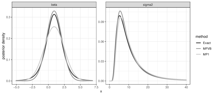
Figure 4: The fitted posteriors for the simple normal sample data described in Section C.7 Example. The posteriors densities corresponding to MP (approach 2) are not plotted because they are exact.

Method	${\mathbb{E}}(\beta\,|\,{\bf y})$	${\mathbb{V}}(\beta\,|\,{\bf y})$	${\mathbb{E}}(\sigma^{2}\,|\,{\bf y})$	${\mathbb{V}}(\sigma^{2}\,|\,{\bf y})$	Iterations
MFVB	0.908	1.47	11.0	120	12
MP1	0.908	2.44	12.2	185	12
MP2	0.908	2.44	12.2	293	17
Exact	0.908	2.44	12.2	293

Table 2: Summary of fits linear models using MFVB and MP methods using the data described in Section C.7 Example. All values have been rounded to 3 significant figures.

Appendix D: MP Derivations for MVN model

In this appendix we provide detailed derivations for all of the material in Section 5.

D.1 Exact posterior distributions for the MVN model

We will next state the full conditional distributions for ${\boldsymbol{\mu}}$ and ${\boldsymbol{\Sigma}}$. These are useful for both the derivation of the MFVB and MP approximations. The full conditional distributions for ${\boldsymbol{\mu}}$ and ${\boldsymbol{\Sigma}}$ are given by

$$\begin{array}[]{rl}{\boldsymbol{\mu}}\,|\,{\bf X},{\boldsymbol{\Sigma}}\par\sim N_{p}\left({\boldsymbol{\mu}}_{n},{\boldsymbol{\Sigma}}/\lambda_{n}\right)\par\par\par\qquad\mbox{and}\qquad\par{\boldsymbol{\Sigma}}\,|\,{\bf X},{\boldsymbol{\mu}}\sim\mbox{IW}_{p}\left({\boldsymbol{\Psi}}({\boldsymbol{\mu}}),\nu_{n}+1\right)\par\end{array}$$

where ${\boldsymbol{\Psi}}({\boldsymbol{\mu}})={\boldsymbol{\Psi}}_{0}+{\bf S}+n(\overline{{\bf x}}-{\boldsymbol{\mu}})(\overline{{\bf x}}-{\boldsymbol{\mu}})^{T}+\lambda_{0}{\boldsymbol{\mu}}{\boldsymbol{\mu}}^{T}$,

$$\begin{array}[]{c}\displaystyle\overline{{\bf x}}={\bf X}^{T}{\bf 1}_{n}/n,\quad\lambda_{n}=\lambda_{0}+n;\quad\nu_{n}=\nu_{0}+n,\\[8.61108pt] {\boldsymbol{\mu}}_{n}=n\overline{{\bf x}}/\lambda_{n},\qquad{\bf S}={\bf X}^{T}{\bf X}-n\overline{{\bf x}}\overline{{\bf x}}^{T},\quad\mbox{and}\quad{\boldsymbol{\Psi}}_{n}={\boldsymbol{\Psi}}_{0}+{\bf S}+n\lambda_{0}/\lambda_{n}\,\overline{{\bf x}}\overline{{\bf x}}^{T}.\end{array}$$ (65)

For this example, we are able to calculate the exact posterior distribution and its corresponding moments. This can be used as a gold standard for comparing the quality of MFVB and MP algorithms. The posterior distribution of ${\boldsymbol{\Sigma}}$ is $\displaystyle{\boldsymbol{\Sigma}}\,|\,{\bf X}\sim\mbox{IW}_{p}\left({\boldsymbol{\Psi}}_{n},\nu_{n}\right)$.

The marginal posterior distribution for ${\boldsymbol{\mu}}$ can be found by noting that if ${\boldsymbol{\mu}}\,|\,{\bf X},{\boldsymbol{\Sigma}}\sim N_{p}\left({\boldsymbol{\mu}}_{n},{\boldsymbol{\Sigma}}/\lambda_{n}\right)$ and ${\boldsymbol{\Sigma}}\,|\,{\bf X}\sim\mbox{IW}_{p}\left({\boldsymbol{\Psi}}_{n},\nu_{n}\right)$ then

$$\begin{array}[]{rl}{\boldsymbol{\mu}}\,|\,{\bf X\par}&\displaystyle\sim t_{p}\left({\boldsymbol{\mu}}_{n},\frac{{\boldsymbol{\Psi}}_{n}}{\lambda_{n}(\nu_{n}-p+1)},\nu_{n}-p+1\right),\end{array}$$

where we have used the usual parametrization of the multivariate $t$ distribution whose density and various expectations are summarised in Appendix A.2 for reference.

D.2 MFVB Derivations for the MVN model

For the MVN model in Section D.9 Example with $q$-density factorization $q({\boldsymbol{\mu}},{\boldsymbol{\Sigma}})=q({\boldsymbol{\mu}},{\boldsymbol{\Sigma}})$, the updates for $q({\boldsymbol{\mu}})$ and $q({\boldsymbol{\Sigma}})$ are derived via

$$\begin{array}[]{rl}q({\boldsymbol{\mu}})&\displaystyle\propto\exp\left[-\tfrac{1}{2}\sum_{i=1}^{n}({\bf x}_{i}-{\boldsymbol{\mu}})^{T}{\boldsymbol{\Sigma}}^{-1}({\bf x}_{i}-{\boldsymbol{\mu}})-\tfrac{1}{2}\lambda_{0}{\boldsymbol{\mu}}^{T}{\boldsymbol{\Sigma}}^{-1}{\boldsymbol{\mu}}\right]\\[12.91663pt] &\displaystyle\propto\exp\left[-\tfrac{\lambda_{n}}{2}{\boldsymbol{\mu}}^{T}{\mathbb{E}}_{q}({\boldsymbol{\Sigma}}^{-1}){\boldsymbol{\mu}}+{\boldsymbol{\mu}}^{T}{\mathbb{E}}_{q}({\boldsymbol{\Sigma}}^{-1})n\overline{{\bf x}}\right]\\[8.61108pt] &\displaystyle\propto\exp\left[-\tfrac{\lambda_{n}\nu_{n}}{2}{\boldsymbol{\mu}}^{T}\widetilde{{\boldsymbol{\Psi}}}^{-1}{\boldsymbol{\mu}}+{\boldsymbol{\mu}}^{T}\widetilde{{\boldsymbol{\Psi}}}^{-1}\nu_{n}n\overline{{\bf x}}\right]\\[8.61108pt] &\displaystyle\sim N_{p}(\widetilde{{\boldsymbol{\mu}}},\widetilde{{\boldsymbol{\Sigma}}})\\[8.61108pt] q({\boldsymbol{\Sigma}})&\displaystyle\propto\exp\left[-\tfrac{n+1+\nu_{0}+p+1}{2}\log\,|\,{\boldsymbol{\Sigma}}\,|\,-\tfrac{1}{2}\mbox{tr}\left\{{\boldsymbol{\Sigma}}^{-1}{\mathbb{E}}_{q}({\boldsymbol{\Psi}}({\boldsymbol{\mu}}))\right\}\right]\\[8.61108pt] &\displaystyle\sim\mbox{IW}_{p}(\widetilde{{\boldsymbol{\Psi}}},\widetilde{\nu}).\par\end{array}$$

where the update for $q({\boldsymbol{\mu}})$ is given by

$$\widetilde{{\boldsymbol{\mu}}}\leftarrow{\boldsymbol{\mu}}_{n};\qquad\widetilde{{\boldsymbol{\Sigma}}}\leftarrow\frac{\widetilde{{\boldsymbol{\Psi}}}}{\lambda_{n}\nu_{n}}$$

and the update for $q({\boldsymbol{\Sigma}})$ is given by

$$\widetilde{{\boldsymbol{\Psi}}}\leftarrow{\boldsymbol{\Psi}}_{n}+\lambda_{n}\widetilde{{\boldsymbol{\Sigma}}};\qquad\widetilde{\nu}\leftarrow\nu_{n}+1.$$

D.3 MFVB for the MVN model

The VB approximation for the MVN normal corresponding to the factorization $q({\boldsymbol{\mu}},{\boldsymbol{\Sigma}})=q({\boldsymbol{\mu}})q({\boldsymbol{\Sigma}})$ have $q$-densities of the forms

$$\begin{array}[]{rl}q({\boldsymbol{\mu}})\par\par&\displaystyle\sim N_{p}(\widetilde{{\boldsymbol{\mu}}},\widetilde{{\boldsymbol{\Sigma}}})\par\qquad\mbox{and}\qquad\par q({\boldsymbol{\Sigma}})\displaystyle\sim\mbox{IW}_{p}(\widetilde{{\boldsymbol{\Psi}}},\widetilde{d}),\par\end{array}$$

where the updates for $\widetilde{{\boldsymbol{\mu}}}$ and $\widetilde{{\boldsymbol{\Sigma}}}$ are provided in equation (66), and the updates for $\widetilde{{\boldsymbol{\Psi}}}$ and $\widetilde{d}$ are provided in equation (67). The iterations of the MFVB algorithm are summarised in Algorithm 8.

Algorithm 8 MFVB method for the MVN model

0:  ${\bf X}\in{\mathbb{R}}^{n\times p}$, ${\boldsymbol{\Psi}}_{0}\in{\mathbb{S}}_{+}^{p}$, $\lambda_{0}>0$, $\nu_{0}>p-1$.

1:  Calculate algorithm constants via (65).

2:  Initialize: $\widetilde{d}\leftarrow\nu_{n}+1$ and $\widetilde{{\boldsymbol{\Psi}}}\leftarrow{\boldsymbol{\Psi}}_{n}$.

3:  repeat

4:     Update $q({\boldsymbol{\mu}})$:

$$\widetilde{{\boldsymbol{\mu}}}\leftarrow{\boldsymbol{\mu}}_{n};\qquad\widetilde{{\boldsymbol{\Sigma}}}\leftarrow\frac{\widetilde{{\boldsymbol{\Psi}}}}{\lambda_{n}\widetilde{d}};$$ (66)

5:     Update $q({\boldsymbol{\Sigma}})$:

$$\widetilde{d}\leftarrow\nu_{n}+1;\qquad\widetilde{{\boldsymbol{\Psi}}}\leftarrow{\boldsymbol{\Psi}}_{n}+\lambda_{n}\widetilde{{\boldsymbol{\Sigma}}};$$ (67)

6:  until convergence criteria is met.

D.4 Result 5

Result 5

Based on the prior choice in (24), the MFVB approximation leads to the exact posterior expectation for ${\boldsymbol{\mu}}$, element-wise underestimation of the posterior variance for ${\boldsymbol{\mu}}$, element-wise underestimation of the posterior expectation for ${\boldsymbol{\Sigma}}$, and provided $\nu_{n}>p+1$, the element-wise posterior variances for ${\boldsymbol{\Sigma}}$ are underestimated.

Throughout Algorithm 8 the values $\widetilde{{\boldsymbol{\mu}}}$ and $\widetilde{d}$ are fixed. Upon termination of Algorithm 8 the following two equations will hold (with high precision) for the variational parameters:

$$\widetilde{{\boldsymbol{\Sigma}}}=\frac{\widetilde{{\boldsymbol{\Psi}}}}{\lambda_{n}\widetilde{d}}\qquad\mbox{and}\qquad\displaystyle\widetilde{{\boldsymbol{\Psi}}}={\boldsymbol{\Psi}}_{n}+\lambda_{n}\widetilde{{\boldsymbol{\Sigma}}}.$$

These constitute two matrix equations and two matrix unknowns. Solving for $\widetilde{{\boldsymbol{\Sigma}}}$ and $\widetilde{{\boldsymbol{\Psi}}}$ we get

$$\widetilde{{\boldsymbol{\Sigma}}}^{*}=\frac{{\boldsymbol{\Psi}}_{n}}{\lambda_{n}\nu_{n}}\qquad\mbox{and}\qquad\widetilde{{\boldsymbol{\Psi}}}^{*}=\frac{\nu_{n}+1}{\nu_{n}}{\boldsymbol{\Psi}}_{n}.$$

Note that the exact posterior variance of ${\boldsymbol{\mu}}$ can be written as

$${\mathbb{V}}_{q}({\boldsymbol{\mu}})=\frac{{\boldsymbol{\Psi}}_{n}}{\lambda_{n}\nu_{n}}\qquad\mbox{and}\qquad{\mathbb{V}}({\boldsymbol{\mu}}\,|\,{\bf X})=\frac{{\boldsymbol{\Psi}}_{n}}{\lambda_{n}(\nu_{n}-p-1)}$$

We can now see that $\lambda_{n}\nu_{n}>\lambda_{n}(\nu_{n}-p-1)$ and hence, $\,|\,[{\mathbb{V}}_{q}({\boldsymbol{\mu}})]_{ij}\,|\,<\,|\,[{\mathbb{V}}({\boldsymbol{\mu}}\,|\,{\bf X})]_{ij}\,|\,$ for all $(i,j)$.

Comparing true and approximate posterior expectations of ${\boldsymbol{\Sigma}}$ we have

$${\mathbb{E}}({\boldsymbol{\Sigma}}\,|\,{\bf X})=\frac{{\boldsymbol{\Psi}}_{n}}{\nu_{n}-p-1}\qquad\mbox{and}\qquad{\mathbb{E}}_{q}({\boldsymbol{\Sigma}})=\frac{\nu_{n}+1}{\nu_{n}}\frac{{\boldsymbol{\Psi}}_{n}}{\nu_{n}-p}$$

The VB estimate is underestimated when

$$\begin{array}[]{rl}\displaystyle\frac{1}{\nu_{n}-p-1}>\frac{\nu_{n}+1}{\nu_{n}}\frac{1}{\nu_{n}-p}&\displaystyle\implies\nu_{n}(\nu_{n}-p)>(\nu_{n}+1)(\nu_{n}-p-1)\\[8.61108pt] &\displaystyle\implies\nu_{n}^{2}-p\nu_{n}>\nu_{n}^{2}-p\nu_{n}-\nu_{n}+\nu_{n}-p-1\\[8.61108pt] &\displaystyle\implies 0>-p-1\end{array}$$

which is always true. Hence, $\,|\,[{\mathbb{E}}({\boldsymbol{\Sigma}}\,|\,{\bf X})]_{ij}\,|\,>\,|\,[{\mathbb{E}}_{q}({\boldsymbol{\Sigma}})]\,|\,$ for all $(i,j)$.

Comparing true and approximate posterior element-wise variances of ${\boldsymbol{\Sigma}}$ we have

$$\begin{array}[]{rl}{\mathbb{E}}{\mathbb{W}}{\mathbb{V}}({\boldsymbol{\Sigma}}\,|\,{\bf X})&\displaystyle=\frac{(\nu_{n}-p+1)({\boldsymbol{\Psi}}_{n}\circ{\boldsymbol{\Psi}}_{n})+(\nu_{n}-p-1)\mbox{dg}({\boldsymbol{\Psi}}_{n})\mbox{dg}({\boldsymbol{\Psi}}_{n})^{T}}{(\nu_{n}-p)(\nu_{n}-p-1)^{2}(\nu_{n}-p-3)}\\[8.61108pt] &\displaystyle=\frac{(\nu_{n}-p+1)[{\mathbb{E}}({\boldsymbol{\Sigma}}\,|\,{\bf X})\circ{\mathbb{E}}({\boldsymbol{\Sigma}}\,|\,{\bf X})]}{(\nu_{n}-p)(\nu_{n}-p-3)}\\[8.61108pt] &\displaystyle\qquad+\frac{(\nu_{n}-p-1)\mbox{dg}({\mathbb{E}}({\boldsymbol{\Sigma}}\,|\,{\bf X}))\mbox{dg}({\mathbb{E}}({\boldsymbol{\Sigma}}\,|\,{\bf X}))^{T}}{(\nu_{n}-p)(\nu_{n}-p-3)}\par\end{array}$$

and

$$\begin{array}[]{rl}{\mathbb{E}}{\mathbb{W}}{\mathbb{V}}_{q}({\boldsymbol{\Sigma}})&\displaystyle=\left(\frac{\nu_{n}+1}{\nu_{n}}\right)^{2}\frac{(\nu_{n}+1-p+1)({\boldsymbol{\Psi}}_{n}\circ{\boldsymbol{\Psi}}_{n})}{(\nu_{n}+1-p)(\nu_{n}+1-p-1)^{2}(\nu_{n}+1-p-3)}\\[8.61108pt] &\displaystyle\qquad+\left(\frac{\nu_{n}+1}{\nu_{n}}\right)^{2}\frac{(\nu_{n}+1-p-1)\mbox{dg}({\boldsymbol{\Psi}}_{n})\mbox{dg}({\boldsymbol{\Psi}}_{n})^{T}}{(\nu_{n}+1-p)(\nu_{n}+1-p-1)^{2}(\nu_{n}+1-p-3)}\par\par\\[8.61108pt] &\displaystyle=\par\frac{(\nu_{n}-p+2)({\mathbb{E}}_{q}({\boldsymbol{\Sigma}})\circ{\mathbb{E}}_{q}({\boldsymbol{\Sigma}}))+(\nu_{n}-p)\mbox{dg}({\mathbb{E}}_{q}({\boldsymbol{\Sigma}}))\mbox{dg}({\mathbb{E}}_{q}({\boldsymbol{\Sigma}}))^{T}}{(\nu_{n}+1-p)(\nu_{n}-p-2)}\\[8.61108pt] \end{array}$$

Hence, $\,|\,[{\mathbb{E}}{\mathbb{W}}{\mathbb{V}}({\boldsymbol{\Sigma}}\,|\,{\bf X})]_{ij}\,|\,>\,|\,[{\mathbb{E}}{\mathbb{W}}{\mathbb{V}}_{q}({\boldsymbol{\Sigma}})]_{ij}\,|\,$ when

$$\frac{(\nu_{n}-p+1)}{(\nu_{n}-p)(\nu_{n}-p-3)}>\frac{(\nu_{n}-p+2)}{(\nu_{n}-p+1)(\nu_{n}-p-2)}$$

and

$$\frac{(\nu_{n}-p-1)}{(\nu_{n}-p)(\nu_{n}-p-3)}>\frac{(\nu_{n}-p)}{(\nu_{n}-p+1)(\nu_{n}-p-2)}$$

The first inequality implies

$$\begin{array}[]{rl}(x+1)^{2}(x-2)>x(x+2)(x-3)&\displaystyle\implies x^{3}-3x-2>x^{3}-x^{2}-6x\\[8.61108pt] &\displaystyle\implies x^{2}+3x-2>0\\[8.61108pt] &\displaystyle\implies x^{2}+3x-2>0\par\end{array}$$

where $x=\nu_{n}-p$ (assuming $x>1$, i.e, $\nu_{n}>p+1)$.

The second inequality implies

$$\begin{array}[]{rl}(x-1)(x+1)(x-2)>x^{2}(x-3)&\displaystyle\implies x^{3}-2x^{2}-x+2>x^{3}-3x^{2}\\[8.61108pt] &\displaystyle\implies x^{2}-x+2>0\par\end{array}$$

which is true provided $x>1$. Hence, $\nu_{n}>p+1$ is sufficient for posterior variances to be element-wise greater than those for MFVB in absolute magnitude.

D.5 Derivations of MP update of $q({\boldsymbol{\mu}})$ for the MVN model

Equating ${\mathbb{E}}_{q}^{MP}({\boldsymbol{\mu}})$ with ${\mathbb{E}}_{q}({\boldsymbol{\mu}})$, and ${\mathbb{V}}_{q}^{MP}({\boldsymbol{\mu}})$ with ${\mathbb{V}}_{q}({\boldsymbol{\mu}})$ we have

$$\widetilde{{\boldsymbol{\mu}}}={\boldsymbol{\mu}}_{n}\qquad\mbox{and}\qquad\widetilde{{\boldsymbol{\Sigma}}}=\frac{\widetilde{\nu}-2}{\widetilde{\nu}\lambda_{n}(d^{*}-1)}\widetilde{{\boldsymbol{\Psi}}}.$$ (68)

where $d^{*}=\widetilde{d}-p$. Using (34) with ${\boldsymbol{\mu}}={\bf 0}$, $a=1$, ${\bf A}={\bf I}$, ${\boldsymbol{\Sigma}}=\widetilde{{\boldsymbol{\Sigma}}}$ and $b=\widetilde{\nu}$ we obtain

$$\begin{array}[]{rl}{\mathbb{E}}_{q}\left[\left\{\|{\boldsymbol{\mu}}-\widetilde{{\boldsymbol{\mu}}}\|^{2}\right\}^{2}\right]&\displaystyle=\frac{\widetilde{\nu}^{2}[2\,\mbox{tr}(\widetilde{{\boldsymbol{\Sigma}}}^{2})+\mbox{tr}(\widetilde{{\boldsymbol{\Sigma}}})^{2}]}{(\widetilde{\nu}-2)(\widetilde{\nu}-4)}\end{array}$$ (69)

and using (68) we have

$$\begin{array}[]{rl}{\mathbb{E}}_{q}\left[\left\{\|{\boldsymbol{\mu}}-\widetilde{{\boldsymbol{\mu}}}\|^{2}\right\}^{2}\right]&\displaystyle=\frac{(\widetilde{\nu}-2)[2\,\mbox{tr}(\widetilde{{\boldsymbol{\Psi}}}^{2})+\mbox{tr}(\widetilde{{\boldsymbol{\Psi}}})^{2}]}{\lambda_{n}^{2}(d^{*}-1)^{2}(\widetilde{\nu}-4)}.\end{array}$$ (70)

Using Corollary 3.1 (i) and (iv) from Rossen (1988) we have

$$\begin{array}[]{rl}{\mathbb{E}}\left[\mbox{tr}({\boldsymbol{\Sigma}}^{2})\right]&\displaystyle=(c_{1}+c_{2})\mbox{tr}(\widetilde{{\boldsymbol{\Psi}}}^{2})+c_{2}\mbox{tr}(\widetilde{{\boldsymbol{\Psi}}})^{2}\qquad\mbox{and}\par\\[4.30554pt] {\mathbb{E}}\left[\mbox{tr}({\boldsymbol{\Sigma}})^{2}\right]&\displaystyle=c_{1}\mbox{tr}(\widetilde{{\boldsymbol{\Psi}}})^{2}+2c_{2}\mbox{tr}(\widetilde{{\boldsymbol{\Psi}}}^{2})\end{array}$$

where $c_{2}^{-1}=d^{*}(d^{*}-1)(d^{*}-3)$, $c_{1}=(d^{*}-2)c_{2}$ and provided $d^{*}>3$. Hence we obtain

$$\begin{array}[]{l}\displaystyle{\mathbb{E}}_{q}\left[{\mathbb{E}}\left\{\left(\|{\boldsymbol{\mu}}-\widetilde{{\boldsymbol{\mu}}}\|^{2}\right)^{2}\,|\,{\bf X},{\boldsymbol{\Sigma}}\right\}\right]\\[8.61108pt] \qquad\displaystyle=\lambda_{n}^{-2}{\mathbb{E}}_{q}\left[\mbox{tr}({\boldsymbol{\Sigma}})^{2}+2\mbox{tr}({\boldsymbol{\Sigma}}^{2})\right]\\[8.61108pt] \qquad\displaystyle=\lambda_{n}^{-2}\left[c_{1}\mbox{tr}(\widetilde{{\boldsymbol{\Psi}}})^{2}+2c_{2}\mbox{tr}(\widetilde{{\boldsymbol{\Psi}}}^{2})\right]+\lambda_{n}^{-2}\left[(2c_{1}+2c_{2})\mbox{tr}(\widetilde{{\boldsymbol{\Psi}}}^{2})+2c_{2}\mbox{tr}(\widetilde{{\boldsymbol{\Psi}}})^{2}\right]\\[8.61108pt] \qquad\displaystyle=\lambda_{n}^{-2}\left(c_{1}+2c_{2}\right)\left[2\mbox{tr}(\widetilde{{\boldsymbol{\Psi}}}^{2})+\mbox{tr}(\widetilde{{\boldsymbol{\Psi}}})^{2}\right]\\[8.61108pt] \qquad\displaystyle=\frac{2\mbox{tr}(\widetilde{{\boldsymbol{\Psi}}}^{2})+\mbox{tr}(\widetilde{{\boldsymbol{\Psi}}})^{2}}{\lambda_{n}^{2}(d^{*}-1)(d^{*}-3)}\end{array}$$ (71)

noting that

$$c_{1}+2c_{2}=(d^{*}-2)c_{2}+2c_{2}=d^{*}c_{2}=\frac{1}{(d^{*}-1)(d^{*}-3)}.$$

Equating (70) and the last expression from (71) and substituting the expression for $\widetilde{{\boldsymbol{\Sigma}}}$ in (68) we obtain

$$\frac{(\widetilde{\nu}-2)\left[2\,\mbox{tr}(\widetilde{{\boldsymbol{\Psi}}}^{2})+\mbox{tr}(\widetilde{{\boldsymbol{\Psi}}})^{2}\right]}{\lambda_{n}^{2}(d^{*}-1)^{2}(\widetilde{\nu}-4)}=\frac{2\mbox{tr}(\widetilde{{\boldsymbol{\Psi}}}^{2})+\mbox{tr}(\widetilde{{\boldsymbol{\Psi}}})^{2}}{\lambda_{n}^{2}(d^{*}-1)(d^{*}-3)}$$

after solving for $\widetilde{\nu}$ we find $\widetilde{\nu}=d^{*}+1=\widetilde{d}-p+1$.

D.6 MP posterior expectation of ${\boldsymbol{\Sigma}}$

Since, ${\boldsymbol{\Sigma}}\,|\,{\bf X},{\boldsymbol{\mu}}\sim\mbox{IW}_{p}({\boldsymbol{\Psi}}({\boldsymbol{\mu}}),\nu_{n}+1)$ the corrected posterior expectation of ${\boldsymbol{\Sigma}}$ is given by

$$\begin{array}[]{rl}{\mathbb{E}}_{q}^{MP}({\boldsymbol{\Sigma}})&\displaystyle={\mathbb{E}}_{q}\left[{\mathbb{E}}({\boldsymbol{\Sigma}}\,|\,{\bf X},{\boldsymbol{\mu}})\right]\par\\[4.30554pt] &\displaystyle=\frac{1}{\nu_{n}+1-p-1}{\mathbb{E}}_{q}\left[{\boldsymbol{\Psi}}({\boldsymbol{\mu}})\right]\par\\[4.30554pt] &\displaystyle=\frac{1}{\nu_{n}-p}\left({\boldsymbol{\Psi}}_{n}+\frac{\widetilde{\nu}}{\widetilde{\nu}-2}\lambda_{n}\widetilde{{\boldsymbol{\Sigma}}}\right)\par\\[8.61108pt] &\displaystyle=\frac{{\bf A}}{\nu_{n}-p}\par\par\par\end{array}$$

where

$${\mathbb{E}}_{q}\left[{\boldsymbol{\Psi}}({\boldsymbol{\mu}})\right]={\boldsymbol{\Psi}}_{n}+\frac{\lambda_{n}\widetilde{\nu}}{\widetilde{\nu}-2}\widetilde{{\boldsymbol{\Sigma}}}\equiv{\bf A}.$$

D.7 MP posterior variance of elements of ${\boldsymbol{\Sigma}}$

In the following derivations the vector ${\bf e}_{i}$ is a vector of zeros, except for the $i$th element which is equal to 1. The matrix ${\bf E}_{ij}$ is a matrix whose elements are 0 except for the $(i,j)$th element which is equal to 1.

The MP variance of the diagonal elements of ${\boldsymbol{\Sigma}}$ are given by

$$\begin{array}[]{rl}{\mathbb{V}}_{q}^{MP}(\Sigma_{ii})&\displaystyle={\mathbb{E}}_{q}\left[{\mathbb{V}}(\Sigma_{ii}\,|\,{\bf X},{\boldsymbol{\mu}})\right]+{\mathbb{V}}_{q}\left[{\mathbb{E}}(\Sigma_{ii}\,|\,{\bf X},{\boldsymbol{\mu}})\right]\\[8.61108pt] &\displaystyle={\mathbb{E}}_{q}\left[\frac{2\{{\boldsymbol{\Psi}}({\boldsymbol{\mu}})\}_{ii}^{2}}{(\nu_{n}-p)^{2}(\nu_{n}-p-2)}\right]+{\mathbb{V}}_{q}\left[\frac{\{{\boldsymbol{\Psi}}({\boldsymbol{\mu}})\}_{ii}}{\nu_{n}-p}\right]\par\\[8.61108pt] &\displaystyle=\frac{2(a_{ii}^{2}+b_{ii})}{(\nu_{n}-p)^{2}(\nu_{n}-p-2)}+\frac{b_{ii}}{(\nu_{n}-p)^{2}}\par\\[8.61108pt] &\displaystyle=\frac{2\,a_{ii}^{2}+(\nu_{n}-p)b_{ii}}{(\nu_{n}-p)^{2}(\nu_{n}-p-2)}\par\par\end{array}$$

where $\{{\boldsymbol{\Psi}}({\boldsymbol{\mu}})\}_{ij}=\psi_{0,ij}+s_{ij}+n(\overline{x}_{i}-\mu_{i})(\overline{x}_{j}-\mu_{j})+\lambda_{0}\mu_{i}\mu_{j}$,

$$a_{ij}\equiv{\mathbb{E}}_{q}\left[\{{\boldsymbol{\Psi}}({\boldsymbol{\mu}})\}_{ij}\right]\qquad\mbox{and}\qquad b_{ij}\equiv{\mathbb{V}}_{q}\left[\{{\boldsymbol{\Psi}}({\boldsymbol{\mu}})\}_{ij}\right].$$

Hence, we can write

$$\begin{array}[]{rl}\mbox{dg}[{\mathbb{E}}{\mathbb{W}}{\mathbb{V}}_{q}^{MP}({\boldsymbol{\Sigma}})]\par&\displaystyle=\frac{2\mbox{dg}({\bf A})^{2}+(\nu_{n}-p)\mbox{dg}({\bf B})}{(\nu_{n}-p)^{2}(\nu_{n}-p-2)}\par\end{array}$$

We have showed ${\mathbb{E}}_{q}[\{{\boldsymbol{\Psi}}({\boldsymbol{\mu}})\}_{ij}]=a_{ij}$, but are yet to derive an expression for $b_{ij}$.

Expanding and completing the square for ${\boldsymbol{\Psi}}({\boldsymbol{\mu}})$ we obtain

$$\begin{array}[]{rl}{\boldsymbol{\Psi}}({\boldsymbol{\mu}})&\displaystyle={\boldsymbol{\Psi}}_{0}+{\bf X}^{T}{\bf X}+n(\overline{{\bf x}}-{\boldsymbol{\mu}})(\overline{{\bf x}}-{\boldsymbol{\mu}})^{T}+\lambda_{0}{\boldsymbol{\mu}}{\boldsymbol{\mu}}^{T}-n\,\overline{{\bf x}}\overline{{\bf x}}^{T}\par\par\par\par\par\\[8.61108pt] &\displaystyle=\lambda_{n}\left({\boldsymbol{\mu}}-{\boldsymbol{\mu}}_{n}\right)\left({\boldsymbol{\mu}}-{\boldsymbol{\mu}}_{n}\right)^{T}-\lambda_{n}{\boldsymbol{\mu}}_{n}{\boldsymbol{\mu}}_{n}^{T}\par\par\par\par\par\par\end{array}$$

Next, we use (35) to calculate

$$\begin{array}[]{rl}{\mathbb{V}}_{q}\left[\displaystyle\{{\boldsymbol{\Psi}}({\boldsymbol{\mu}})\}_{ij}\right]&\displaystyle=\lambda_{n}^{2}{\mathbb{V}}_{q}\left[(\mu_{i}-\widetilde{\mu}_{i})(\mu_{j}-\widetilde{\mu}_{j})\right]\par\\[8.61108pt] &\displaystyle=\lambda_{n}^{2}{\mathbb{V}}_{q}\left[({\boldsymbol{\mu}}-\widetilde{{\boldsymbol{\mu}}}){\bf e}_{i}{\bf e}_{j}^{T}({\boldsymbol{\mu}}-\widetilde{{\boldsymbol{\mu}}})\right]\par\\[8.61108pt] &\displaystyle=\lambda_{n}^{2}{\mathbb{V}}_{q}\left[({\boldsymbol{\mu}}-\widetilde{{\boldsymbol{\mu}}}){\bf E}_{ij}({\boldsymbol{\mu}}-\widetilde{{\boldsymbol{\mu}}})\right]\end{array}$$

The diagonal elements of ${\bf B}$ are given by

$$\begin{array}[]{rl}{\mathbb{V}}_{q}\left[\displaystyle\{{\boldsymbol{\Psi}}({\boldsymbol{\mu}})\}_{ii}\right]\par&\displaystyle=\lambda_{n}^{2}{\mathbb{V}}_{q}\left[({\boldsymbol{\mu}}-\widetilde{{\boldsymbol{\mu}}}){\bf E}_{ii}({\boldsymbol{\mu}}-\widetilde{{\boldsymbol{\mu}}})\right]\par\\[8.61108pt] &\displaystyle=\lambda_{n}^{2}\Bigg{[}\frac{2\widetilde{\nu}^{2}\,\mbox{tr}({\bf E}_{ii}\widetilde{{\boldsymbol{\Sigma}}}{\bf E}_{ii}\widetilde{{\boldsymbol{\Sigma}}})}{(\widetilde{\nu}-2)(\widetilde{\nu}-4)}+\frac{2\widetilde{\nu}^{2}\,\mbox{tr}({\bf E}_{ii}\widetilde{{\boldsymbol{\Sigma}}})^{2}}{(\widetilde{\nu}-2)^{2}(\widetilde{\nu}-4)}\Bigg{]}\par\\[12.91663pt] &\displaystyle=\lambda_{n}^{2}\left[\frac{2\widetilde{\nu}^{2}\,\widetilde{\Sigma}_{ii}^{2}}{(\widetilde{\nu}-2)(\widetilde{\nu}-4)}+\frac{2\widetilde{\nu}^{2}\,\widetilde{\Sigma}_{ii}^{2}}{(\widetilde{\nu}-2)^{2}(\widetilde{\nu}-4)}\right]\par\\[12.91663pt] &\displaystyle=\frac{2\lambda_{n}^{2}\widetilde{\nu}^{2}(\widetilde{\nu}-1)\,\widetilde{\Sigma}_{ii}^{2}}{(\widetilde{\nu}-2)^{2}(\widetilde{\nu}-4)}\par\par\par\\[8.61108pt] &\displaystyle\equiv b_{ii}\par\end{array}$$

Hence,

$${\bf b}\equiv\mbox{dg}\left[{\mathbb{E}}{\mathbb{W}}{\mathbb{V}}_{q}\left\{{\boldsymbol{\Psi}}({\boldsymbol{\mu}})\right\}\right]=\frac{2\lambda_{n}^{2}\widetilde{\nu}^{2}(\widetilde{\nu}-1)}{(\widetilde{\nu}-2)^{2}(\widetilde{\nu}-4)}\mbox{dg}(\widetilde{{\boldsymbol{\Sigma}}})^{2}.$$

D.8 Result 6

Result 6

There are two solution of the moment equations (25)-(28) for the MP method for the MVN model described by Algorithm 5.

• One solution corresponds to $\widetilde{{\boldsymbol{\Psi}}}^{*}={\boldsymbol{\Psi}}_{n}$, $\widetilde{d}^{*}=\nu_{n}$,

  $$\begin{array}[]{c}\widetilde{{\boldsymbol{\mu}}}^{*}={\boldsymbol{\mu}}_{n},\qquad\displaystyle\widetilde{{\boldsymbol{\Sigma}}}^{*}=\frac{{\boldsymbol{\Psi}}_{n}}{\lambda_{n}(\nu_{n}-p+1)}\quad\mbox{and}\quad\widetilde{\nu}^{*}=\nu_{n}-p+1.\end{array}$$

  These correspond to the parameters of the exact posterior distribution.

• The second solution corresponds to $\widetilde{{\boldsymbol{\mu}}}\leftarrow{\boldsymbol{\mu}}_{n}$, $\widetilde{d}=p+3$,

  $$\widetilde{{\boldsymbol{\Psi}}}=\frac{2{\boldsymbol{\Psi}}_{n}}{\nu_{n}-p-1},\quad\widetilde{{\boldsymbol{\Sigma}}}=\frac{{\boldsymbol{\Psi}}_{n}}{2\lambda_{n}(\nu_{n}-p-1)}\quad\mbox{and}\quad\widetilde{\nu}=4.$$

  leading to an inexact estimation of the posterior distribution.

Consider the set of consistency conditions as the set of equations (25)-(28). Matching ${\mathbb{V}}^{MP}_{q}({\boldsymbol{\mu}})$ with the ${\mathbb{V}}_{q}({\boldsymbol{\mu}})$ leads to the equations

$$\begin{array}[]{rl}\displaystyle\frac{\widetilde{{\boldsymbol{\Psi}}}}{\lambda_{n}(\widetilde{d}-p-1)}&\displaystyle=\frac{\widetilde{\nu}\widetilde{{\boldsymbol{\Sigma}}}}{\widetilde{\nu}-2}.\end{array}$$

Equating ${\mathbb{E}}_{q}^{MP}({\boldsymbol{\Sigma}})$ with ${\mathbb{E}}_{q}({\boldsymbol{\Sigma}})$ and the above equation we get

$$\begin{array}[]{rl}\displaystyle\frac{\widetilde{{\boldsymbol{\Psi}}}}{\widetilde{d}-p-1}&\displaystyle=\frac{1}{\nu_{n}-p}\left[{\boldsymbol{\Psi}}_{n}+\frac{\widetilde{{\boldsymbol{\Psi}}}}{\widetilde{d}-p-1}\right].\end{array}$$

Solving for $\widetilde{{\boldsymbol{\Psi}}}$ we obtain

$$\widetilde{{\boldsymbol{\Psi}}}=\frac{\widetilde{d}-p-1}{\nu_{n}-p-1}{\boldsymbol{\Psi}}_{n}.$$

Hence, we can write the expressions for ${\bf A}$ and $\mbox{dg}({\bf B})$ as

$$\begin{array}[]{c}\displaystyle{\bf A}={\boldsymbol{\Psi}}_{n}+\frac{\widetilde{{\boldsymbol{\Psi}}}}{(\widetilde{d}-p-1)}=\frac{\nu_{n}-p}{\widetilde{d}-p-1}\widetilde{{\boldsymbol{\Psi}}}\end{array}$$

and

$$\begin{array}[]{rl}\mbox{dg}({\bf B})&\displaystyle=\frac{\lambda_{n}^{2}\widetilde{\nu}^{2}(\widetilde{\nu}-1)}{(\widetilde{\nu}-2)^{2}(\widetilde{\nu}-4)}2\mbox{dg}(\widetilde{{\boldsymbol{\Sigma}}})^{2}\\[8.61108pt] &\displaystyle=\frac{1}{(\widetilde{d}-p-1)^{2}}\frac{(\widetilde{\nu}-1)}{(\widetilde{\nu}-4)}2\mbox{dg}(\widetilde{{\boldsymbol{\Psi}}})^{2}\par\\[8.61108pt] &\displaystyle=\frac{(\widetilde{\nu}-1)}{(\nu_{n}-p)^{2}(\widetilde{\nu}-4)}2\mbox{dg}({\bf A})^{2}.\par\end{array}$$

Hence, the moment matching equation for $\widetilde{d}$ can be written as

$$\begin{array}[]{rl}\displaystyle\widetilde{d}&\displaystyle=\frac{\displaystyle 2{\bf 1}^{T}[\mbox{dg}({\mathbb{E}}_{q}^{MP}({\boldsymbol{\Sigma}}))^{2}]}{\mbox{tr}[{\mathbb{E}}{\mathbb{W}}{\mathbb{V}}_{q}^{MP}({\boldsymbol{\Sigma}})]}+p+3\\[8.61108pt] &\displaystyle=\frac{\displaystyle\frac{2}{(\nu_{n}-p)^{2}}{\bf 1}^{T}[\mbox{dg}({\bf A})^{2}]}{\displaystyle\frac{2{\bf 1}^{T}[\mbox{dg}({\bf A})^{2}]+(\nu_{n}-p)\mbox{tr}({\bf B})}{(\nu_{n}-p)^{2}(\nu_{n}-p-2)}}+p+3\par\\[8.61108pt] &\displaystyle=(\nu_{n}-p-2)\frac{\displaystyle 2{\bf 1}^{T}[\mbox{dg}({\bf A})^{2}]}{\displaystyle 2{\bf 1}^{T}[\mbox{dg}({\bf A})^{2}]+(\nu_{n}-p)\mbox{tr}({\bf B})}+p+3\end{array}$$

Substituting the above expressions for ${\bf A}$ in terms of $\nu_{n}$, $\widetilde{d}$, p and $\widetilde{{\boldsymbol{\Psi}}}$ we have

$$\begin{array}[]{rl}\widetilde{d}&\displaystyle=\frac{\displaystyle(\nu_{n}-p-2)}{\displaystyle 1+\frac{(\widetilde{\nu}-1)}{(\nu_{n}-p)(\widetilde{\nu}-4)}\par}+p+3\par\\[8.61108pt] &\displaystyle=(\nu_{n}-p-2)\frac{\displaystyle(\nu_{n}-p)(\widetilde{\nu}-4)}{\displaystyle(\nu_{n}-p)(\widetilde{\nu}-4)+(\widetilde{\nu}-1)}+p+3\par\par\\[8.61108pt] &\displaystyle=(\nu_{n}-p-2)\left[1-\frac{\displaystyle(\widetilde{\nu}-1)}{\displaystyle(\nu_{n}-p)(\widetilde{\nu}-4)+(\widetilde{\nu}-1)}\right]+p+3\par\par\\[17.22217pt] &\displaystyle=\nu_{n}+1-\frac{\displaystyle(\widetilde{\nu}-1)(\nu_{n}-p-2)}{\displaystyle(\nu_{n}-p)(\widetilde{\nu}-4)+(\widetilde{\nu}-1)}\par\par\\[8.61108pt] &\displaystyle=\nu_{n}+1-\frac{\displaystyle(\widetilde{d}-p)(\nu_{n}-p-2)}{\displaystyle(\nu_{n}-p)(\widetilde{d}-p-3)+(\widetilde{d}-p)}\par\end{array}$$

where the last line follows from using $\widetilde{\nu}=\widetilde{d}-p+1$. Letting $x=\widetilde{d}-p$ and $y=\nu_{n}-p$ leads to the equation

$$\begin{array}[]{rl}x&\displaystyle=y+1-\frac{\displaystyle x(y-2)}{y(x-3)+x}\\ &\displaystyle=y+1-\frac{\displaystyle x(y+1)-3x}{\displaystyle x(y+1)-3y}\end{array}$$

Multiplying by $x(y+1)-3y$, expanding, simplifying, and grouping by powers of $x$, and dividing through by $y+1$ we have

$$x^{2}-(y+3)x+3y=0$$

The solutions are:

$$x=\frac{y+3\pm(y-3)}{2}=y\,\mbox{ or }\,3$$

and so $\widetilde{d}=\nu_{n}$ or $\widetilde{d}=p+3$.

If $\widetilde{d}=\nu_{n}$ then $\widetilde{{\boldsymbol{\Psi}}}={\boldsymbol{\Psi}}_{n}$ and the MP approximation matches the exact solution.

However, If $\widetilde{d}=p+3$ then

$$\widetilde{{\boldsymbol{\Psi}}}=\frac{2{\boldsymbol{\Psi}}_{n}}{\nu_{n}-p-1}.$$

and so $\widetilde{{\boldsymbol{\mu}}}={\boldsymbol{\mu}}_{n}$,

$$\widetilde{{\boldsymbol{\Sigma}}}=\frac{{\boldsymbol{\Psi}}_{n}}{2\lambda_{n}(\nu_{n}-p-1)}\quad\mbox{and}\quad\widetilde{\nu}=4.$$

Leading to inexact $q$-densities.

D.9 Example

Suppose we draw $n=4$ samples from ${\bf x}_{i}\stackrel{{\scriptstyle\scriptsize iid}}{{\sim}}N_{2}({\boldsymbol{\mu}},{\boldsymbol{\Sigma}})$ with

$${\boldsymbol{\mu}}=\left[\begin{array}[]{r}-1\\ 1\end{array}\right]\qquad\mbox{and}\qquad{\boldsymbol{\Sigma}}=\left[\begin{array}[]{cc}1&0.75\\ 0.75&1\end{array}\right]$$

with summary statistics

$$\overline{{\bf x}}=\left[\begin{array}[]{r}-0.9724726\\ 1.3202681\end{array}\right]\qquad\mbox{and}\qquad{\bf S}=\left[\begin{array}[]{rr}0.8144316&0.5688416\\ 0.5688416&1.9682059\\ \end{array}\right].$$

Again, we have chosen the sample size to be small in order to see the biggest differences between MFVB and Exact methods.

The fitted values of the $q$-densities are summarised in Table 3. Figure 5 displays the posterior density estimates for MFVB against the exact posterior distributions. The posterior covariances for ${\boldsymbol{\mu}}$ are given by

$${\mathbb{E}}_{q}^{VB}({\boldsymbol{\mu}})=\left[\begin{array}[]{cc}0.065&0.020\\ 0.020&0.106\end{array}\right]\qquad\mbox{and}\qquad{\mathbb{E}}({\boldsymbol{\mu}}|{\bf X})=\left[\begin{array}[]{cc}0.114&0.035\\ 0.035&0.186\end{array}\right],$$

and the element-wise variances for ${\boldsymbol{\Sigma}}$ are given by

$${\mathbb{E}}_{q}^{VB}({\boldsymbol{\Sigma}})=\left[\begin{array}[]{cc}0.116&0.085\\ 0.085&0.310\end{array}\right]\qquad\mbox{and}\qquad{\mathbb{E}}{\mathbb{W}}{\mathbb{V}}({\boldsymbol{\Sigma}}|{\bf X})=\left[\begin{array}[]{cc}0.208&0.148\\ 0.148&0.557\end{array}\right],$$

showing the exact posterior variances for ${\boldsymbol{\mu}}$ are 1.75 times bigger than MFVB estimates, and the that MFVB estimates, and the exact posterior element-wise variances for ${\boldsymbol{\Sigma}}$ are 1.73-1.79 times bigger than the corresponding MFVB estimates.

Method	$\widetilde{\nu}$	$\widetilde{d}$	$\widetilde{\Sigma}_{11}$	$\widetilde{\Sigma}_{12}$	$\widetilde{\Sigma}_{22}$	$\widetilde{\Psi}_{11}$	$\widetilde{\Psi}_{12}$	$\widetilde{\Psi}_{22}$	Iterations
MFVB		8	0.065	0.0198	0.106	2.08	0.635	3.41	9
MP	6	7	0.114	0.0347	0.186	1.82	0.556	2.99	22
Exact	6	7	0.114	0.0347	0.186	1.82	0.556	2.99

Table 3: Summary of fits for the MVN model using MFVB and MP methods for the data described in Section D.9 Example. The values for $\widetilde{{\boldsymbol{\mu}}}$ are not shown because they are exact for all methods.

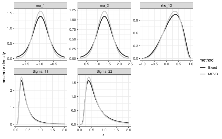
Figure 5: The fitted posteriors for the MVN model using data described in Section D.9 Example. The posteriors densities corresponding to MP are not plotted because they are exact.

Appendix E: Derivations for probit regression

In this appendix we provide detailed derivations for all of the material in Section 6.

E.1 Derivations for MFVB

The derivation, except for very minor changes can be found in Ormerod and Wand (2010) (setting ${\bf y}={\bf 1}_{n}$, and using ${\bf Z}=\mbox{diag}(2{\bf y}-1){\bf X}$ in place of ${\bf X}$). We refer the interested reader there. The MFVB approximation corresponding to $q({\boldsymbol{\beta}},{\bf a})=q({\boldsymbol{\beta}})\,q({\bf a})$ is

$$\begin{array}[]{lcl}q({\boldsymbol{\beta}})\displaystyle=N(\widetilde{{\boldsymbol{\mu}}}_{\beta},\widetilde{{\boldsymbol{\Sigma}}}_{\beta})&\quad\mbox{and}&q(a_{i})\displaystyle=\mbox{TN}_{+}(\widetilde{\mu}_{a,i},1),\qquad i=1,\ldots,n,\end{array}$$

where the update for $q({\boldsymbol{\beta}})$ is given by $\widetilde{{\boldsymbol{\mu}}}_{\beta}\leftarrow{\bf S}{\bf Z}^{T}{\mathbb{E}}_{q}({\bf a})$, and $\widetilde{{\boldsymbol{\Sigma}}}_{\beta}\leftarrow{\bf S}$. Algorithm 9 summarises the MFVB algorithm for the probit regression model. Algorithm 9 is very fast (per iteration) due to the fact that the matrix ${\bf S}$ needs to be only calculated once outside the main loop.

Algorithm 9 MFVB for probit regression

0:  ${\bf y}\in{\mathbb{R}}^{n}$, ${\bf X}\in{\mathbb{R}}^{n\times p}$ and initial value for $\widetilde{{\boldsymbol{\mu}}}_{\beta}$.

1:  Set ${\bf Z}=\mbox{diag}(2{\bf y}-{\bf 1}_{n}){\bf X}$, and ${\bf S}=({\bf Z}^{T}{\bf Z}+{\bf D})^{-1}$

2:  repeat

3:     Update $q({\bf a})$ via $\widetilde{{\boldsymbol{\mu}}}_{a}\leftarrow{\bf Z}\widetilde{{\boldsymbol{\mu}}}_{\beta}$

4:     Update $q({\boldsymbol{\beta}})$ via $\widetilde{{\boldsymbol{\mu}}}_{\beta}\leftarrow{\bf S}{\bf Z}^{T}(\widetilde{{\boldsymbol{\mu}}}_{a}+\zeta_{1}(\widetilde{{\boldsymbol{\mu}}}_{a}));\,\widetilde{{\boldsymbol{\Sigma}}}_{\beta}\leftarrow{\bf S};$

5:  until convergence criteria is met

E.2 Linear Response Variational Bayes

At this point we could apply the LRVB approach of Giordano et al. (2015) to correct the variances of MFVB. This approach can be viewed as a post-hoc correction to MFVB. Direct application of LRVB is not possible since $p(a_{i})$ is not differentiable. Instead we absorb the MFVB update for $q({\bf a})$ into $q({\boldsymbol{\beta}})$. This is equivalent for using the SEM method of Meng and Rubin (1991). Indeed Giordano et al. (2015) state that for two parameter sets LRVB and SEM are equivalent.

We now argue that, for this model, LRVB leads to an approximation equivalent to the Laplace approximation. To see this first note that Algorithm 9 is identical to the Bayesian Expectation Maximization approach applied to the probit model. Applying the SEM method to the probit regression model we have

$$\begin{array}[]{rl}M({\boldsymbol{\mu}}_{\beta})&={\bf S}{\bf Z}[{\bf Z}{\boldsymbol{\mu}}_{\beta}+\zeta_{1}({\bf Z}{\boldsymbol{\mu}}_{\beta})],\qquad\mbox{and}\\[8.61108pt] DM({\boldsymbol{\mu}}_{\beta})&=\displaystyle\frac{\partial M({\boldsymbol{\mu}}_{\beta})}{d{\boldsymbol{\mu}}_{\beta}}={\bf S}{\bf Z}[{\bf I}_{n}+\mbox{diag}\{\zeta_{2}({\bf Z}{\boldsymbol{\mu}}_{\beta})\}]{\bf Z}.\end{array}$$

Then

$${\mathbb{V}}^{SEM}({\boldsymbol{\mu}})={\bf S}[{\bf I}-DM({\boldsymbol{\mu}}_{\beta})]^{-1}=[{\bf Z}\mbox{diag}\{-\zeta_{2}({\bf Z}{\boldsymbol{\mu}}_{\beta})\}{\bf Z}+{\bf D}]^{-1}$$

which is the posterior covariance estimate corresponding to the Laplace approximation when ${\boldsymbol{\mu}}_{\beta}$ is equal to the posterior mode.

E.3 Calculating $\xi_{d}(\mu,\sigma^{2})$

Fast, stable and accurate estimation of $\xi_{d}(\mu,\sigma^{2})$ is pivotal for the MP-QUAD method, as well as direct optimization approaches of the ELBO for and. We only focus on the case when $d\in\{0,1,2\}$ since these are the only cases needed for MP-QUAD and GVB. We employ two different strategies for evaluating $\xi_{d}(\mu,\sigma^{2})$: a Taylor series approximation, and composite trapezoidal integration.

A Taylor series expansion of the integrand around $x=\mu$ in (31) leads to

$$\xi_{d}(\mu,\sigma^{2})=\sum_{k=0}^{\infty}\frac{\zeta_{d+2k}(\mu)\,\sigma^{2k}}{2^{k}k!}$$ (72)

where $\xi_{d}(\mu,\sigma^{2})$ is the Gaussian smoothed version of $\zeta_{d}(x)$. The derivatives of $\zeta_{1}(t)$ and its derivative are given by $\zeta_{1}(t)=\phi(t)/\Phi(t)$, $\zeta_{2}(t)=-t\,\zeta_{1}(t)-\zeta_{1}(t)^{2}$ and for $k=3,4,\ldots$ the function $\zeta_{k}(t)$ can be calculated recursively via the formula

$$\zeta_{k}(t)=-\left[\,t\,\zeta_{k-1}(t)+(k-2)\zeta_{k-2}(t)\,\right]-\sum_{j=0}^{k-2}\binom{k-2}{j}\,\zeta_{1+j}(t)\,\zeta_{k-1-j}(t).$$

Empirically we have found that the series (72) does not converges for all $\mu$, $\sigma^{2}$ and $d$ in particular when $\sigma^{2}>1$. Note that for the probit regression model high leverage points lead to large $\sigma^{2}$. Nevertheless, the terms in the series (72) converge very rapidly to 0, especially when $\sigma^{2}<\tau$ for some chosen $\tau<1$. Later, in Section E.4 Proof of Result 1 , we will argue under mild regularity conditions that $\sigma^{2}$ values will be $O_{p}(n^{-1})$ so that each additional term on the right hand side of (72) gives an order of magnitude more accuracy. Truncating (72) at just 5 terms is much faster than numerical quadrature with accuracies up to 6-8 significant figures of accuracy. Adaptive quadrature methods use in general many more function evaluations.

For $\sigma^{2}>\tau$ we use composite trapezoidal quadrature. This involves A. finding good starting points, B. finding the mode of the integrand, C. finding the effective domain of the integrand, and D. applying composite trapezoidal quadrature. Note that because the effective domains will be the same for $d\in\{0,1,2\}$ we focus on the case when $d=1$ since this is the easiest to deal with.

Finding good starting points: We work on the log-scale to avoid underflow issues. Let $f(x)$ be the log of the integrand for $\xi_{1}(\mu,\sigma^{2})$, i.e., up to additive constants

$$f(x)=-\frac{x^{2}}{2}-\log\Phi(x)-\frac{(x-\mu)^{2}}{2\sigma^{2}}$$

with $f^{\prime}(x)=-x-\zeta_{1}(x)-(x-\mu)/\sigma^{2}$ and $f^{\prime\prime}(x)=-1-\zeta_{2}(x)=1/\sigma^{2}$.

We wish to find the maximizer of $f(x)$ with respect to $x$, corresponding to the mode of the integrand of $\xi_{1}$. We consider three different starting points

1. For positive large $x$ we have $\log\Phi(x)\approx 0$ leading to the approximate mode $x_{1}=\mu/(1+\sigma^{2})$.

2. For $x$ close to zero we perform a Talyor series for $\log\Phi(x)$ around $x=0$ leading to $\log\Phi(x)\approx-\log(2)-\sqrt{2/\pi}x-x^{2}/\pi$ leading to the approximate mode $x_{2}=(\mu-\sigma^{2}\sqrt{2/\pi})/(\sigma^{2}(1-\pi/2)+1)$.

3. For negative large $x$ we have $\log\Phi(x)\sim\log\phi(x)-\log(-x)$ leading to the approximate mode $x_{3}=-\sqrt{\mu+\sigma^{2}}$ (provided $\mu+\sigma^{2}>0$).

We evaluate $f(x)$ at $x_{1}$, $x_{2}$ and $x_{3}$ (providing it exists), and choose the point with the largest value as the starting point, $x^{(0)}$.

Finding the mode of the integrand: We then find the mode using Newton’s method $x^{(t+1)}=x^{(t)}-f^{\prime}(x^{(t)})/f^{\prime\prime}(x^{(t)})$. When $|f^{\prime}(x^{(t)})/f^{\prime\prime}(x^{(t)})|<\tau_{\mbox{\scriptsize mode}}$ we stop. We have used $\tau_{\mbox{\scriptsize mode}}=10^{-3}$ in our implementation. Let $x^{*}$ denote the mode.

Finding the effective domain: Let $s=-1/\sqrt{f^{\prime\prime}(x^{*})}$. To find the effective domain we take steps to the left and to the right of the mode $x^{*}$ until $f(x^{*}-sL)$ and $f(x^{*}+sR)$ are both less than $\tau_{\mbox{\scriptsize ED}}\times f(x^{*})$ for some integers $L$ and $R$. We have used $\tau_{\mbox{\scriptsize ED}}=10^{-3}$ in our implementation.

Composite trapezoid quadrature: We then perform composite trapezoidal quadrature between $a=x^{*}-sL$ and $b=x^{*}+sR$ with $N+1$ equally spaced quadrature points ${\displaystyle a=x_{0}<x_{1}<\cdots<x_{N-1}<x_{N}=b}$ and approximate the integral by

$$\int_{a}^{b}F(x)\,dx\approx\sum_{k=1}^{N}\frac{F(x_{k-1})+F(x_{k})}{2}\Delta x_{k}\qquad\mbox{where}\qquad F(x)=\zeta_{d}(x)\phi(x;\mu;\sigma^{2})$$

and $\Delta x_{k}=x_{k}-x_{k-1}$. Note that this approach is extremely effective, particularly for integrals when all derivatives of $F$ are close to $0$ on the boundary of the integral. In such cases the trapezoid rule can have exponential rates of convergence (see Section 4.5.1 of Press et al., 2007, for details). We have found $N=50$ to be sufficiently accurate and have used this value in our implementation.

E.4 Proof of Result 1

We will make the following assumptions

1. The likelihood and prior are given by (29) and ${\boldsymbol{\beta}}\sim N_{p}({\bf 0},{\bf D}^{-1})$ respectively.

2. Algorithm 8 is applied.

3. ${\bf x}_{i}\in{\mathbb{R}}^{p}$, $i=1,\ldots,n$ are independent identically distributed random vectors (with $p$ fixed) such that

   $${\mathbb{E}}({\bf x}_{i})={\boldsymbol{\mu}}_{x}\qquad\mbox{and}\qquad{\mathbb{V}}({\bf x}_{i})={\boldsymbol{\Sigma}}_{x}$$

   where all elements of ${\boldsymbol{\mu}}_{x}\in{\mathbb{R}}^{p}$ and ${\boldsymbol{\Sigma}}_{x}$ are finite with ${\boldsymbol{\Sigma}}_{x}\in{\mathcal{S}}_{+}^{p}$.

Assumption (A1) implies that $p({\bf y},{\boldsymbol{\beta}})$ is log-concave (strictly) and so there exists a unique maximizer to $p({\bf y},{\boldsymbol{\beta}})$, with posterior mode $\widehat{{\boldsymbol{\beta}}}$, and with Laplace approximation

$${\boldsymbol{\beta}}\,|\,{\bf y}\stackrel{{\scriptstyle\mbox{\small approx.}}}{{\sim}}N_{p}\left(\widehat{{\boldsymbol{\beta}}},({\bf Z}^{T}\mbox{diag}(-\zeta_{2}({\bf Z}\widehat{{\boldsymbol{\beta}}})){\bf Z}+{\bf D})^{-1}\right).$$

Using (A3) we know from the strong law of large numbers that

$${\bf X}^{T}{\bf X}=\sum_{i=1}^{n}{\bf x}_{i}{\bf x}_{i}^{T}=n\left[{\boldsymbol{\mu}}_{x}{\boldsymbol{\mu}}_{x}^{T}+{\boldsymbol{\Sigma}}_{x}+O_{p}^{m}(n^{-1/2})\right]$$

where ${\bf A}=O_{p}^{m}(n^{-1})$ denotes that all elements of ${\bf A}$ are $O_{p}(n^{-1})$. Then

$$\begin{array}[]{rl}{\bf S}=({\bf Z}^{T}{\bf Z}+{\bf D})^{-1}&\displaystyle=({\bf X}^{T}{\bf X}+{\bf D})^{-1}\\ &\displaystyle=\left[n\left({\boldsymbol{\mu}}_{x}{\boldsymbol{\mu}}_{x}^{T}+{\boldsymbol{\Sigma}}_{x}+O_{p}^{m}(n^{-1/2})\right)+{\bf D}\right]^{-1}\\ &\displaystyle=n^{-1}\left({\boldsymbol{\mu}}_{x}{\boldsymbol{\mu}}_{x}^{T}+{\boldsymbol{\Sigma}}_{x}\right)^{-1}+O_{p}^{m}(n^{-3/2})\par\end{array}$$

where the last line follows from a Taylor series argument. Hence, ${\bf S}=O_{p}^{m}(n^{-1})$.

We now consider the iterations of Algorithm 9 and Algorithm 6. Let

$$\widetilde{{\boldsymbol{\mu}}}_{\beta,VB}^{(t)}\qquad\mbox{and}\qquad\widetilde{{\boldsymbol{\mu}}}_{a,VB}^{(t)}$$

be the values of $\widetilde{{\boldsymbol{\mu}}}_{\beta}$, and $\widetilde{{\boldsymbol{\mu}}}_{a}$ respectively of Algorithm 9 at for iteration $t$. Similarly, let

$$\widetilde{{\boldsymbol{\mu}}}_{\beta,MP}^{(t)},\qquad\widetilde{{\boldsymbol{\Sigma}}}_{\beta,MP}^{(t)},\qquad\mbox{and}\qquad\widetilde{{\boldsymbol{\mu}}}_{a,MP}^{(t)}$$

be the values of $\widetilde{{\boldsymbol{\mu}}}_{\beta}$, $\widetilde{{\boldsymbol{\Sigma}}}_{\beta}$, and $\widetilde{{\boldsymbol{\mu}}}_{a}$ respectively of Algorithm 6 at for iteration $t$.

Next we note that the MFVB algorithm for probit regression (Algorithm 9), is identical to using Bayesian Expectation Maximization to find the posterior mode (for probit regression, not in general) (see Dunson et al. (2013), Chapter 10). Hence, the sequence $\widetilde{{\boldsymbol{\mu}}}^{(t)}_{\beta,VB}$ converges to the posterior mode. However, as argued by Consonni and Marin (2007), MFVB underestimates the posterior variance.

Merging the steps of Algorithm 9 the update for $\widetilde{{\boldsymbol{\mu}}}_{\beta,VB}$ may be written as

$$\widetilde{{\boldsymbol{\mu}}}_{\beta,VB}^{(t+1)}={\bf S}{\bf Z}^{T}({\bf Z}\widetilde{{\boldsymbol{\mu}}}_{\beta,VB}^{(t)}+\zeta_{1}({\bf Z}\widetilde{{\boldsymbol{\mu}}}_{\beta,VB}^{(t)}))$$

Similarly, merging the steps of Algorithm 6 the updates can be written in the form

$$\begin{array}[]{rl}\widetilde{{\boldsymbol{\mu}}}_{\beta,MP}^{(t+1)}&\displaystyle\leftarrow{\bf S}{\bf Z}^{T}\left[{\bf Z}\widetilde{{\boldsymbol{\mu}}}_{\beta,MP}^{(t)}\par+\xi_{1}({\bf Z}\widetilde{{\boldsymbol{\mu}}}_{\beta},\mbox{dg}({\bf Z}\widetilde{{\boldsymbol{\Sigma}}}_{\beta,MP}^{(t)}{\bf Z}^{T}))\par\right]\par\par\\[8.61108pt] \widetilde{{\boldsymbol{\Sigma}}}_{\beta,MP}^{(t+1)}&\displaystyle\leftarrow{\bf S}+{\bf S}{\bf Z}^{T}\,[\,{\bf I}_{n}+\mbox{diag}\{\xi_{2}({\bf Z}\widetilde{{\boldsymbol{\mu}}}_{\beta,MP}^{(t)},\mbox{dg}({\bf Z}\widetilde{{\boldsymbol{\Sigma}}}_{\beta,MP}^{(t)}{\bf Z}^{T}))\}\,]\,{\bf Z}{\bf S}\\[4.30554pt] &\displaystyle\qquad+{\bf S}{\bf Z}^{T}\,[\,{\bf I}_{n}+\mbox{diag}\{\zeta_{2}({\bf Z}\widetilde{{\boldsymbol{\mu}}}_{\beta,MP}^{(t)})\}\,]\,{\bf Z}\widetilde{{\boldsymbol{\Sigma}}}_{\beta,MP}^{(t)}{\bf Z}^{T}\,[\,{\bf I}_{n}+\mbox{diag}\{\zeta_{2}({\bf Z}\widetilde{{\boldsymbol{\mu}}}_{\beta,MP}^{(t)})\}\,]\,{\bf Z}{\bf S}\end{array}$$

Suppose that $\widetilde{{\boldsymbol{\mu}}}_{\beta,VB}^{(0)}=\widetilde{{\boldsymbol{\mu}}}_{\beta,MP}^{(0)}$ and $\widetilde{{\boldsymbol{\Sigma}}}_{\beta,VB}^{(0)}=\widetilde{{\boldsymbol{\Sigma}}}_{\beta,MP}^{(0)}={\bf S}$ so that MFVB and MP methods start at the same initial values. We will now show, via induction, that if

$$\widetilde{{\boldsymbol{\mu}}}_{\beta,MP}^{(t)}-\widetilde{{\boldsymbol{\mu}}}_{\beta,VB}^{(t)}=O_{p}^{v}(n^{-1})\quad\mbox{and}\quad\widetilde{{\boldsymbol{\Sigma}}}_{\beta,MP}^{(t)}=O_{p}^{m}(n^{-1})$$ (73)

then

$$\widetilde{{\boldsymbol{\mu}}}_{\beta,MP}^{(t+1)}-\widetilde{{\boldsymbol{\mu}}}_{\beta,VB}^{(t+1)}=O_{p}^{v}(n^{-1})\quad\mbox{and}\quad\widetilde{{\boldsymbol{\Sigma}}}_{\beta,MP}^{(t+1)}=O_{p}^{m}(n^{-1})$$

where $O_{p}^{v}(n^{-1})$ is interpreted as a vector whose elements are all $O_{p}(n^{-1})$.

Note that (73) holds for $t=0$ by the choice of initional con

Assuming (73) we have ${\bf z}_{i}^{T}\widetilde{{\boldsymbol{\Sigma}}}_{\beta,MP}^{(t)}{\bf z}_{i}=O_{p}(n^{-1})$ and so

$$\xi_{d}({\bf Z}\widetilde{{\boldsymbol{\mu}}}_{\beta,MP}^{(t)},\mbox{dg}({\bf Z}\widetilde{{\boldsymbol{\Sigma}}}_{\beta,MP}^{(t)}{\bf Z}^{T}))=\zeta_{d}({\bf Z}\widetilde{{\boldsymbol{\mu}}}_{\beta,MP}^{(t)})+O_{p}^{v}(n^{-1}).$$

for $d\in\{1,2\}$ via a Taylor series argument. Hence,

$$\begin{array}[]{l}\widetilde{{\boldsymbol{\mu}}}_{\beta,MP}^{(t+1)}-\widetilde{{\boldsymbol{\mu}}}_{\beta,VB}^{(t+1)}\\ \quad\displaystyle={\bf S}{\bf Z}^{T}\left[{\bf Z}\widetilde{{\boldsymbol{\mu}}}_{\beta,MP}^{(t)}+\zeta_{1}({\bf Z}\widetilde{{\boldsymbol{\mu}}}_{\beta,MP}^{(t)})+O_{p}^{v}(n^{-1})\right]-{\bf S}{\bf Z}^{T}\left[{\bf Z}\widetilde{{\boldsymbol{\mu}}}_{\beta,VB}^{(t)}+\zeta_{1}({\bf Z}\widetilde{{\boldsymbol{\mu}}}_{\beta,VB}^{(t)})\right]\par\\[8.61108pt] \quad\displaystyle={\bf S}{\bf Z}^{T}{\bf Z}\left[\widetilde{{\boldsymbol{\mu}}}_{\beta,MP}^{(t)}-\widetilde{{\boldsymbol{\mu}}}_{\beta,VB}^{(t)}\right]+{\bf S}{\bf Z}^{T}\left[\zeta_{1}({\bf Z}\widetilde{{\boldsymbol{\mu}}}_{\beta,MP}^{(t)})-\zeta_{1}({\bf Z}\widetilde{{\boldsymbol{\mu}}}_{\beta,VB}^{(t)})\right]+O_{p}^{v}(n^{-1})\par\par\\[8.61108pt] \quad\displaystyle={\bf S}{\bf Z}^{T}{\bf Z}\left[\widetilde{{\boldsymbol{\mu}}}_{\beta,MP}^{(t)}-\widetilde{{\boldsymbol{\mu}}}_{\beta,VB}^{(t)}\right]\\[8.61108pt] \quad\displaystyle\qquad+{\bf S}{\bf Z}^{T}{\bf Z}\left[\zeta_{2}({\bf Z}\widetilde{{\boldsymbol{\mu}}}_{\beta,VB}^{(t)})\circ(\widetilde{{\boldsymbol{\mu}}}_{\beta,MP}^{(t)}-\widetilde{{\boldsymbol{\mu}}}_{\beta,VB}^{(t)})\right]+O_{p}^{v}(n^{-1})\par\\[8.61108pt] \quad\displaystyle=O_{p}^{v}(n^{-1})\par\par\end{array}$$

since ${\bf S}{\bf Z}^{T}{\bf Z}=O_{p}^{m}(1)$. Similarly,

$$\begin{array}[]{l}\widetilde{{\boldsymbol{\Sigma}}}_{\beta,MP}^{(t+1)}\\ \quad\displaystyle={\bf S}+{\bf S}{\bf Z}^{T}\left[\,{\bf I}_{n}+\mbox{diag}\left\{\zeta_{2}({\bf Z}\widetilde{{\boldsymbol{\mu}}}_{\beta,MP}^{(t)})+O_{p}^{v}(n^{-1})\right\}\right]\,{\bf Z}{\bf S}\\[4.30554pt] \quad\displaystyle\qquad+{\bf S}{\bf Z}^{T}\left[\,{\bf I}_{n}+\mbox{diag}\left\{\zeta_{2}({\bf Z}\widetilde{{\boldsymbol{\mu}}}_{\beta,MP}^{(t)})\right\}\right]\,{\bf Z}\widetilde{{\boldsymbol{\Sigma}}}_{\beta,MP}^{(t)}{\bf Z}^{T}\left[\,{\bf I}_{n}+\mbox{diag}\left\{\zeta_{2}({\bf Z}\widetilde{{\boldsymbol{\mu}}}_{\beta,MP}^{(t)})\right\}\right]\,{\bf Z}{\bf S\par}\\[8.61108pt] \quad\displaystyle={\bf S}+{\bf S}{\bf Z}^{T}\left[\,{\bf I}_{n}+{\bf W}^{(t)}\right]\,{\bf Z}{\bf S}\\[8.61108pt] \quad\displaystyle\qquad+{\bf S}{\bf Z}^{T}\left[\,{\bf I}_{n}+{\bf W}^{(t)}\right]\,{\bf Z}\widetilde{{\boldsymbol{\Sigma}}}_{\beta,MP}^{(t)}{\bf Z}^{T}\left[\,{\bf I}_{n}+{\bf W}^{(t)}\right]\,{\bf Z}{\bf S}+O_{p}^{m}(n^{-2})\par\\[8.61108pt] \quad\displaystyle=O_{p}^{m}(n^{-1})\par\end{array}$$

where ${\bf W}^{(t)}=\mbox{diag}\{\zeta_{2}({\bf Z}\widetilde{{\boldsymbol{\mu}}}_{\beta,VB}^{(t)})\}$. Hence, if $\widetilde{{\boldsymbol{\mu}}}_{\beta,MP}^{(t)}-\widetilde{{\boldsymbol{\mu}}}_{\beta,VB}^{(t)}=O_{p}^{v}(n^{-1})$ and $\widetilde{{\boldsymbol{\Sigma}}}_{\beta,MP}^{(t)}=O_{p}^{m}(n^{-1})$ then $\widetilde{{\boldsymbol{\mu}}}_{\beta,MP}^{(t+1)}-\widetilde{{\boldsymbol{\mu}}}_{\beta,VB}^{(t+1)}=O_{p}^{v}(n^{-1})$ and $\widetilde{{\boldsymbol{\Sigma}}}_{\beta,MP}^{(t+1)}=O_{p}^{m}(n^{-1})$.

Now since $\widetilde{{\boldsymbol{\mu}}}_{\beta,VB}^{(t)}\to\widehat{{\boldsymbol{\beta}}}$ as $t\to\infty$ upon convergence we have

$$\widetilde{{\boldsymbol{\mu}}}_{\beta,MP}=\widehat{{\boldsymbol{\beta}}}+O_{p}^{v}(n^{-1})$$

Upon convergence of the algorithm we have $\widetilde{{\boldsymbol{\Sigma}}}_{\beta,MP}^{(t)}=\widetilde{{\boldsymbol{\Sigma}}}_{\beta,MP}^{(t+1)}\equiv\widetilde{{\boldsymbol{\Sigma}}}_{\beta,MP}^{*}$ and

$$\begin{array}[]{rl}\widetilde{{\boldsymbol{\Sigma}}}_{\beta,MP}^{*}\par&\displaystyle={\bf S}+{\bf S}{\bf Z}^{T}\left[\,{\bf I}_{n}+{\bf W}^{*}\right]\,{\bf Z}{\bf S}\\[8.61108pt] &\displaystyle\qquad+{\bf S}{\bf Z}^{T}\left[{\bf I}_{n}+{\bf W}^{*}\right]\,{\bf Z}\widetilde{{\boldsymbol{\Sigma}}}_{\beta,MP}^{*}{\bf Z}^{T}\left[{\bf I}_{n}+{\bf W}^{*}\right]\,{\bf Z}{\bf S}+O_{p}^{m}(n^{-2})\par\par\end{array}$$

where ${\bf W}^{*}=\mbox{diag}[\zeta_{2}({\bf Z}\widehat{{\boldsymbol{\beta}}})]$. Multiplying both sides by ${\bf S}^{-1}$ and rearranging we have

$$\begin{array}[]{l}({\bf Z}^{T}{\bf Z}+{\bf D})\widetilde{{\boldsymbol{\Sigma}}}_{\beta,MP}^{*}({\bf Z}^{T}{\bf Z}+{\bf D})-({\bf Z}^{T}{\bf Z}+{\bf Z}^{T}{\bf W}^{*}{\bf Z})\widetilde{{\boldsymbol{\Sigma}}}_{\beta,MP}^{*}({\bf Z}^{T}{\bf Z}+{\bf Z}^{T}{\bf W}^{*}{\bf Z})\\[8.61108pt] \qquad\displaystyle={\bf Z}^{T}{\bf Z}+{\bf D}+{\bf Z}^{T}{\bf Z}+{\bf Z}^{T}{\bf W}^{*}{\bf Z}+O_{p}^{m}(n^{-2})\par\end{array}$$

which we can write as

$$\begin{array}[]{l}({\bf Z}^{T}{\bf Z}+{\bf D}+{\bf Z}^{T}{\bf Z}+{\bf Z}^{T}{\bf W}^{*}{\bf Z})\widetilde{{\boldsymbol{\Sigma}}}_{\beta,MP}^{*}(-{\bf Z}^{T}{\bf W}^{*}{\bf Z}+{\bf D})\\[8.61108pt] \qquad\displaystyle={\bf Z}^{T}{\bf Z}+{\bf D}+{\bf Z}^{T}{\bf Z}+{\bf Z}^{T}{\bf W}^{*}{\bf Z}+O_{p}^{m}(n^{-2})\par\end{array}$$

left multiplying by $({\bf Z}^{T}{\bf Z}+{\bf D}+{\bf Z}^{T}{\bf Z}+{\bf Z}^{T}{\bf W}^{*}{\bf Z})^{-1}$ and right multiplying by $(-{\bf Z}^{T}{\bf W}^{*}{\bf Z}+{\bf D})^{-1}$ we have

$$\begin{array}[]{l}\widetilde{{\boldsymbol{\Sigma}}}_{\beta,MP}^{*}=\left[{\bf Z}^{T}\mbox{diag}\{-\zeta_{2}({\bf Z}^{T}\widehat{{\boldsymbol{\beta}}})\}{\bf Z}+{\bf D}\right]^{-1}+O_{p}^{m}(n^{-2})\par\end{array}$$

and the result is proved.

E.3 Methods compared

In what is to follow let

$$f({\boldsymbol{\beta}})=\log p({\bf y},{\boldsymbol{\beta}})={\bf 1}_{n}^{T}\log\Phi({\bf Z}{\boldsymbol{\beta}})-\tfrac{1}{2}{\boldsymbol{\beta}}^{T}{\bf D}{\boldsymbol{\beta}}+\mbox{constants}$$

so that the gradient vector and Hessian matrix are given by

$${\bf g}({\boldsymbol{\beta}})={\bf Z}^{T}\zeta_{1}({\bf Z}{\boldsymbol{\beta}})-{\bf D}{\boldsymbol{\beta}}\qquad\mbox{and}\qquad{\bf H}({\boldsymbol{\beta}})={\bf Z}^{T}\mbox{diag}(\zeta_{1}({\bf Z}{\boldsymbol{\beta}})){\bf Z}-{\bf D}$$

respectively.

Laplace’s method: Here we maximize the log-likelihood via Newton-Raphson iterations, i.e., starting at ${\boldsymbol{\beta}}^{(0)}$ ($t=0$),

$${\boldsymbol{\beta}}^{(t+1)}={\boldsymbol{\beta}}^{(t)}-[{\bf H}({\boldsymbol{\beta}}^{(t)})]^{-1}{\bf g}({\boldsymbol{\beta}}^{(t)})$$

Upon convergence $q({\boldsymbol{\beta}})=\phi({\boldsymbol{\beta}};\widetilde{{\boldsymbol{\mu}}},\widetilde{{\boldsymbol{\Sigma}}})$ where $\widetilde{{\boldsymbol{\mu}}}={\boldsymbol{\beta}}^{*}$ and $\widetilde{{\boldsymbol{\Sigma}}}=[-{\bf H}({\boldsymbol{\beta}}^{*})]^{-1}$ and ${\boldsymbol{\beta}}^{*}$ is the value of ${\boldsymbol{\beta}}^{(t)}$ at convergence.

Gaussian Variational Bayes (GVB): Let $q({\boldsymbol{\beta}})=\phi({\boldsymbol{\beta}};\widetilde{{\boldsymbol{\mu}}},\widetilde{{\boldsymbol{\Sigma}}})$. Then, using (1) and similar ideas to the derivation of (31), the corresponding ELBO is given by

$$\mbox{ELBO}={\bf 1}_{n}^{T}\xi_{0}({\bf Z}\widetilde{{\boldsymbol{\mu}}},\mbox{dg}({\bf Z}\widetilde{{\boldsymbol{\Sigma}}}{\bf Z}^{T}))-\tfrac{1}{2}\widetilde{{\boldsymbol{\mu}}}^{T}{\bf D}\widetilde{{\boldsymbol{\mu}}}-\tfrac{1}{2}\mbox{tr}({\bf D}\widetilde{{\boldsymbol{\Sigma}}})+\tfrac{1}{2}\log|\widetilde{{\boldsymbol{\Sigma}}}|+\mbox{constants}.$$

Then using results from Opper and Archambeau (2009) we have

$$\begin{array}[]{rcl}\nabla_{\widetilde{{\boldsymbol{\mu}}}}\mbox{ELBO}&={\mathbb{E}}_{q}[{\bf g}({\boldsymbol{\beta}})]&={\bf Z}^{T}\xi_{1}({\bf Z}\widetilde{{\boldsymbol{\mu}}},\mbox{dg}({\bf Z}\widetilde{{\boldsymbol{\Sigma}}}{\bf Z}^{T}))-{\bf D}\widetilde{{\boldsymbol{\mu}}},\\[8.61108pt] \nabla_{\widetilde{{\boldsymbol{\mu}}}\widetilde{{\boldsymbol{\mu}}}}^{2}\mbox{ELBO}&={\mathbb{E}}_{q}[{\bf H}({\boldsymbol{\beta}})]&={\bf Z}^{T}\mbox{diag}(\xi_{2}({\bf Z}\widetilde{{\boldsymbol{\mu}}},\mbox{dg}({\bf Z}\widetilde{{\boldsymbol{\Sigma}}}{\bf Z}^{T}))){\bf Z}-{\bf D},\par\end{array}$$

and

$$\frac{\partial\mbox{ELBO}}{\partial\widetilde{\Sigma}_{ij}}=\frac{1}{2}\mbox{tr}\left[\left\{\widetilde{{\boldsymbol{\Sigma}}}^{-1}+{\mathbb{E}}_{q}({\bf H}({\boldsymbol{\beta}}))\right\}\frac{\partial\widetilde{{\boldsymbol{\Sigma}}}}{\partial\widetilde{\Sigma}_{ij}}\right].$$ (74)

We compared two optimization approaches:

• Direct Optimization: Maximization the ELBO with respect to $\widetilde{{\boldsymbol{\mu}}}$, and the parameters of a (dense, full rank, positive definite) $\widetilde{{\boldsymbol{\Sigma}}}$ requires optimization over $O(d^{2})$ parameters. We used the BFGS algorithm in the function optim() in R a first order method that uses gradient information to construct an approximation of the inverse Hessian. However, this approach uses $O(d^{4})$ memory, and so we recommend a limited memory Quasi-Newton method, see for example Byrd et al. (1995), when $d$ is large. The objective function is given by the ELBO, the gradient is given by the expression for ${\mathbb{E}}_{q}[{\bf g}({\boldsymbol{\beta}})]$ above, and the gradient with respect to the parameterization of $\widetilde{{\boldsymbol{\Sigma}}}$ we give now. We use a Cholesky factorization parameterization of $\widetilde{{\boldsymbol{\Sigma}}}$ of the form $\widetilde{{\boldsymbol{\Sigma}}}={\bf C}^{T}{\bf C}$ where ${\bf C}$ is an upper triangular matrix of the form

  $${\bf C}=\left[\begin{array}[]{ccccc}e^{c_{11}}&c_{12}&c_{13}&\ldots&c_{1d}\\ 0&e^{c_{22}}&c_{23}&\ldots&c_{2d}\\ 0&0&e^{c_{33}}&\ldots&c_{3d}\\ \vdots&\vdots&\vdots&\ddots&\vdots\\ 0&0&0&\ldots&e^{c_{dd}}\\ \end{array}\right]$$

  This parameterization been used in many places. Exponentiation of the diagonal to ensure positiveness of ${\bf C}$. Note that Tan and Nott (2018) use a similar parameterization of the inverse of $\widetilde{{\boldsymbol{\Sigma}}}$ which can be useful when ${\bf H}({\boldsymbol{\beta}})$ is either sparse or has some other structure that can be exploited. The gradient vector can then be calculated using

  $$\frac{\partial\mbox{ELBO}}{\partial c_{ij}}=\left[{\bf C}\left\{\widetilde{{\boldsymbol{\Sigma}}}^{-1}+{\bf Z}^{T}\mbox{diag}(\xi_{2}({\bf Z}\widetilde{{\boldsymbol{\mu}}},\mbox{dg}({\bf Z}\widetilde{{\boldsymbol{\Sigma}}}{\bf Z}^{T}))){\bf Z}-{\bf D}\right\}\right]_{ij}\exp[c_{ij}I(i=j)]$$

  for the diagonal and upper diagonal elements of ${\bf C}$.

• Double Stochastic Variational Bayes (DSVB): As stated in the main paper, a stochastic gradient descent approach (based on code from Tran et al. (2020) (is used with the default settings stated there) modified to use the reparameterization trick of Titsias and Lázaro-Gredilla (2014) for increased numeric stability. This method only requires $f({\boldsymbol{\beta}})$ and ${\bf g}({\boldsymbol{\beta}})$ and not their expectations with respect to $q$, which can sometimes be difficult to evaluate quickly, stably, and accurately.

The main difficulty with direct optimization or DSVB is the maximizing the lower bound with respect to $\widetilde{{\boldsymbol{\Sigma}}}$ since for a dense, positive definite covariance matrix (with no additional structure), the number of parameters required is $O(p^{2})$ which can slow down computations for even moderately high dimensions. The next method we consider partially avoids this problem.

Delta Method Variational Bayes (DMVB): Following Wang and Blei (2013), a first order delta method approximation of the ELBO leads to (ignoring additive constants)

$$\begin{array}[]{rl}\mbox{AELBO}(\widetilde{{\boldsymbol{\mu}}},\widetilde{{\boldsymbol{\Sigma}}})&\displaystyle={\bf 1}_{n}^{T}\zeta_{0}({\bf Z}\widetilde{{\boldsymbol{\mu}}})-\tfrac{1}{2}\widetilde{{\boldsymbol{\mu}}}^{T}{\bf D}\widetilde{{\boldsymbol{\mu}}}+\tfrac{1}{2}\mbox{tr}\left[\widetilde{{\boldsymbol{\Sigma}}}\left\{{\bf Z}^{T}\mbox{diag}(\zeta_{2}({\bf Z}\widetilde{{\boldsymbol{\mu}}})){\bf Z}-{\bf D}\right\}\right]+\tfrac{1}{2}\log|\widetilde{{\boldsymbol{\Sigma}}}|.\end{array}$$

Fixing $\widetilde{{\boldsymbol{\mu}}}$, the derivatives of the approximate ELBO (AELBO) with respect to the parameters of $\widetilde{{\boldsymbol{\Sigma}}}$ are

$$\frac{\partial\mbox{AELBO}}{\partial\widetilde{\Sigma}_{ij}}=\frac{1}{2}\mbox{tr}\left[\left\{\widetilde{{\boldsymbol{\Sigma}}}^{-1}+{\bf Z}^{T}\mbox{diag}(\zeta_{2}({\bf Z}\widetilde{{\boldsymbol{\mu}}})){\bf Z}-{\bf D}\right\}\frac{\partial\widetilde{{\boldsymbol{\Sigma}}}}{\partial\widetilde{\Sigma}_{ij}}\right]$$

Setting the right hand side to zero for all $(i,j)$ and solving for $\widetilde{{\boldsymbol{\Sigma}}}$ leads to the unique solution (for all $\widetilde{{\boldsymbol{\mu}}})$

$$\widetilde{{\boldsymbol{\Sigma}}}^{*}(\widetilde{{\boldsymbol{\mu}}})=\left[{\bf Z}^{T}\mbox{diag}(-\zeta_{2}({\bf Z}\widetilde{{\boldsymbol{\mu}}})){\bf Z}+{\bf D}\right]^{-1}.$$

Substituting $\widetilde{{\boldsymbol{\Sigma}}}^{*}(\widetilde{{\boldsymbol{\mu}}})$ into the AELBO leads to (ignoring additive constants)

$$\begin{array}[]{rl}\mbox{AELBO}(\widetilde{{\boldsymbol{\mu}}},\widetilde{{\boldsymbol{\Sigma}}}^{*}(\widetilde{{\boldsymbol{\mu}}}))&\displaystyle={\bf 1}_{n}^{T}\zeta_{0}({\bf Z}\widetilde{{\boldsymbol{\mu}}})-\tfrac{1}{2}\widetilde{{\boldsymbol{\mu}}}^{T}{\bf D}\widetilde{{\boldsymbol{\mu}}}-\tfrac{1}{2}\log|{\bf Z}^{T}\mbox{diag}(-\zeta_{2}({\bf Z}\widetilde{{\boldsymbol{\mu}}})){\bf Z}+{\bf D}|,\end{array}$$

which is a function of $\widetilde{{\boldsymbol{\mu}}}$ only. We can then maximize $\mbox{AELBO}(\widetilde{{\boldsymbol{\mu}}},\widetilde{{\boldsymbol{\Sigma}}}^{*})$ directly rather with respect to $\widetilde{{\boldsymbol{\mu}}}$ which only involves $O(p)$ parameters, rather than $O(p^{2})$ parameters. The gradient vector with respect to $\widetilde{{\boldsymbol{\mu}}}$ is then

$$\frac{\mbox{AELBO}(\widetilde{{\boldsymbol{\mu}}},\widetilde{{\boldsymbol{\Sigma}}}^{*}(\widetilde{{\boldsymbol{\mu}}}))}{\partial\mu_{j}}=[{\bf Z}^{T}\zeta_{1}({\bf Z}\widetilde{{\boldsymbol{\mu}}})-{\bf D}\widetilde{{\boldsymbol{\mu}}}]_{j}+\tfrac{1}{2}\mbox{dg}({\bf Z}\widetilde{{\boldsymbol{\Sigma}}}^{*}(\widetilde{{\boldsymbol{\mu}}}){\bf Z}^{T})^{T}[{\bf Z}_{j}\circ\zeta_{3}({\bf Z}\widetilde{{\boldsymbol{\mu}}})],$$

where ${\bf Z}_{j}$ is the $j$th column of ${\bf Z}$. We can then use any first order optimization method, e.g., BFGS. to maximize $\mbox{AELBO}(\widetilde{{\boldsymbol{\mu}}},\widetilde{{\boldsymbol{\Sigma}}}^{*}(\widetilde{{\boldsymbol{\mu}}}))$ with respect to $\widetilde{{\boldsymbol{\mu}}}$. Let $\widetilde{{\boldsymbol{\mu}}}^{*}$ be this maximizer, then $\widetilde{{\boldsymbol{\Sigma}}}^{*}=\left[{\bf Z}^{T}\mbox{diag}(-\zeta_{2}({\bf Z}\widetilde{{\boldsymbol{\mu}}}^{*})){\bf Z}+{\bf D}\right]^{-1}$. This approach has the advantages that $\widetilde{{\boldsymbol{\Sigma}}}$ does not need to be optimized over (and so scales well with $p$), and does not require expectations with respect to $q$ of $f({\boldsymbol{\beta}})$, ${\bf g}({\boldsymbol{\beta}})$ or ${\bf H}({\boldsymbol{\beta}})$.

References

- Albert and Chib (1993) Albert, J.H., Chib, S., 1993. Bayesian analysis of binary and polychotomous response data. Journal of the American Statistical Association 88, 669–679.
- Azzalini (2021) Azzalini, A., 2021. The R package sn: The skew-normal and related distributions such as the skew- and the SUN (version 2.0.0). Università di Padova, Italia.
- Bishop (2006) Bishop, C.M., 2006. Pattern Recognition and Machine Learning. Springer, New York.
- Blei et al. (2017) Blei, D.M., Kucukelbir, A., McAuliffe, J.D., 2017. Variational inference: A review for statisticians. Journal of the American Statistical Association 112, 859–877.
- Boyd and Vandenberghe (2004) Boyd, S., Vandenberghe, L., 2004. Convex Optimization. Cambridge University Press, Cambridge.
- Braun and McAuliffe (2010) Braun, M., McAuliffe, J., 2010. Variational inference for large-scale models of discrete choice. Journal of the American Statistical Association 105, 324–335.
- Byrd et al. (1995) Byrd, R.H., Lu, P., Nocedal, J., Zhu, C., 1995. A limited memory algorithm for bound constrained optimization. SIAM Journal on Scientific Computing 16, 1190–1208.
- Challis and Barber (2013) Challis, E., Barber, D., 2013. Gaussian Kullback-Leibler approximate inference. Journal of Machine Learning Research 14, 2239–2286.
- Chopin and Ridgway (2017) Chopin, N., Ridgway, J., 2017. Leave Pima Indians alone: Binary regression as a benchmark for Bayesian computation. Statistical Science 32, 64 – 87.
- Consonni and Marin (2007) Consonni, G., Marin, J.M., 2007. Mean-field variational approximate Bayesian inference for latent variable models. Computational Statistics & Data Analysis 52, 790–798.
- Dresdner et al. (2021) Dresdner, G., Shekhar, S., Pedregosa, F., Locatello, F., Rätsch, G., 2021. Boosting variational inference with locally adaptive step-sizes. arXiv:2105.09240.
- Dua and Graff (2017) Dua, D., Graff, C., 2017. UCI machine learning repository. URL: http://archive.ics.uci.edu/ml.
- Dunson et al. (2013) Dunson, D., Rubin, D., Carlin, J., Gelman, A., Stern, H., Vehtari, A., 2013. Bayesian Data Analysis (3rd ed.). Chapman and Hall/CRC.
- Faes et al. (2011) Faes, C., Ormerod, J., Wand, M., 2011. Variational Bayesian inference for parametric and nonparametric regression With missing data. Journal of the American Statistical Association 106, 959–971.
- Friston et al. (2007) Friston, K., Mattout, J., Trujillo-Barreto, N., Ashburner, J., Penny, W., 2007. Variational free energy and the Laplace approximation. NeuroImage 34, 220–234.
- Frühwirth-Schnatter et al. (2009) Frühwirth-Schnatter, S., Frühwirth, R., Held, L., Rue, H., 2009. Improved auxiliary mixture sampling for hierarchical models of non-Gaussian data. Statistics and Computing 19, 479–492.
- Giordano et al. (2015) Giordano, R., Broderick, T., Jordan, M.I., 2015. Linear response methods for accurate covariance estimates from mean field variational Bayes, in: NIPS, pp. 1441–1449.
- Grimmett and Stirzaker (2001) Grimmett, G., Stirzaker, S., 2001. Probability Theory and Random Processes (3rd ed.). Cambridge University Press, Cambridge.
- Guo et al. (2016) Guo, F., Wang, X., Fan, K., Broderick, T., Dunson, D.B., 2016. Boosting variational inference. CoRR abs/1611.05559.
- Hall et al. (2002) Hall, P., Humphreys, K., Titterington, D.M., 2002. On the adequacy of variational lower bound functions for likelihood-based inference in Markovian models With missing values. Journal of the Royal Statistical Society, Series B 64, 549–564.
- Han et al. (2016) Han, S., Liao, X., Dunson, D., Carin, L., 2016. Variational Gaussian copula inference, in: Gretton, A., Robert, C.C. (Eds.), Proceedings of the 19th International Conference on Artificial Intelligence and Statistics, pp. 829–838.
- Hoffman and Gelman (2014) Hoffman, M.D., Gelman, A., 2014. The no-U-turn sampler: Adaptively setting path lengths in Hamiltonian Monte Carlo. Journal of Machine Learning Research 15, 1593–1623.
- Horn and Johnson (2012) Horn, R.A., Johnson, C.R., 2012. Matrix Analysis. 2nd ed., Cambridge University Press, USA.
- Huggins et al. (2020) Huggins, J., Kasprzak, M., Campbell, T., Broderick, T., 2020. Validated variational inference via practical posterior error bounds, in: Chiappa, S., Calandra, R. (Eds.), Proceedings of the Twenty Third International Conference on Artificial Intelligence and Statistics, PMLR. pp. 1792–1802.
- Humphreys and Titterington (2000) Humphreys, K., Titterington, D.M., 2000. Approximate Bayesian inference for simple mixtures, in: Bethlehem, J.G., van der Heijden, P.G.M. (Eds.), COMPSTAT, Physica-Verlag HD, Heidelberg. pp. 331–336.
- Jaakkola and Jordan (1997) Jaakkola, T.S., Jordan, M.I., 1997. A variational approach to Bayesian logistic regression models and their extensions, in: Madigan, D., Smyth, P. (Eds.), Proceedings of the Sixth International Workshop on Artificial Intelligence and Statistics, pp. 283–294.
- Kingma and Welling (2014) Kingma, D.P., Welling, M., 2014. Auto-encoding variational bayes.
- Kucukelbir et al. (2017) Kucukelbir, A., Tran, D., Ranganath, R., Gelman, A., Blei, D.M., 2017. Automatic differentiation variational inference. Journal of Machine Learning Research 18, 430–474.
- Kullback and Leibler (1951) Kullback, S., Leibler, R.A., 1951. On information and sufficiency. The Annals of Mathematical Statistics 22, 79–86.
- Locatello et al. (2018) Locatello, F., Khanna, R., Ghosh, J., Ratsch, G., 2018. Boosting variational inference: an optimization perspective, in: Storkey, A., Perez-Cruz, F. (Eds.), Proceedings of the Twenty-First International Conference on Artificial Intelligence and Statistics, pp. 464–472.
- Luts and Ormerod (2014) Luts, J., Ormerod, J.T., 2014. Mean field variational Bayesian inference for support vector machine classification. Computational Statistics & Data Analysis 73, 163–176.