Abstract

The aim of Machine Unlearning (MU) is to allow for the removal of the contribution of a given data point from a training procedure. Federated Unlearning (FU) consists in extending MU to unlearn a given client’s contribution from a federated training routine. While a number of FU methods have been proposed, we currently lack a general approach providing formal unlearning guarantees, while allowing scalability and generalization beyond the convex assumption on the clients loss functions. In this work we present Informed Federated Unlearning (IFU), a novel FU theory applying to both convex and non-convex optimization regimes. Upon receiving an unlearning request from a given client, IFU identifies the optimal FL iteration from which FL has to be reinitialized, with unlearning guarantees obtained through a randomized perturbation mechanism. The theory of IFU is also extended to account for sequential unlearning requests (SIFU). Experimental results on different tasks and datasets show that our approach leads to more efficient unlearning procedures as compared to basic re-training and state-of-the-art FU approaches.

1 Introduction

With the emergence of new data regulations, such as the EU General Data Protection Regulation (GDPR) Voigt and Von dem Bussche, (2017) and the California Consumer Privacy Act (CCPA) Harding et al., (2019), the storage and processing of sensitive personal data is often the subject of strict constraints and restrictions. In particular, the “right to be forgotten” states that personal data must be erased upon request from the concerned individuals, with subsequent potential implications on machine learning models trained by using this data. Machine Unlearning (MU) is an emerging discipline that studies methods that aim at removing the contribution of a given data instance used to train a machine learning model. Current MU approaches are essentially based on routines that modify the model weights in order to guarantee the “unlearning” of a given data point, i.e. to obtain a model equivalent to a hypothetical one trained without this data point Cao and Yang, (2015); Bourtoule et al., (2021).

Motivated by data governance and confidentiality concerns, Federated Learning (FL) has gained popularity in the last years to allow data owners to collaboratively learn a model without sharing their respective data. Among the different FL approaches, federated averaging (FedAvg) has emerged as the most popular optimization scheme McMahan et al., 2017a . An optimization round of FedAvg requires data owners, also called clients, to receive the current global model from the server, which is updated by performing a fixed amount of Stochastic Gradient Descent (SGD) steps before sending back the resulting model. The new global model is then created as the weighted average of the client updates. The FL communication design ensures clients that their data is solely used to compute their model update, while established theory guarantees convergence of the model to a stationary point of the clients’ joint optimization problem Wang et al., (2020); Li et al., (2020).

With the current deployments of FL in the real-world, it is of crucial importance to extend MU to guarantee the unlearning of clients wishing to opt-out from a collaborative training routine. This is not straightforward, since current MU schemes have been proposed essentially in the centralized learning setting, and cannot be seamlessly applied to the federated one. For example, several MU methods require the estimation of the Hessian of the loss function Guo et al., (2020); Izzo et al., (2021); Golatkar et al., 2020a ; Golatkar et al., 2020b ; Golatkar et al., (2021), an operation which is computationally expensive and intractable for high dimensional models. Moreover, sharing the Hessian would require clients to share with the server additional information about their data, thus exposing the federated setting to information leakage and attacks, for example under the form of model inversion Fredrikson et al., (2015). Alternative MU methods draw from the concept of differential privacy Dwork and Roth, (2014) and are based on Gaussian noise perturbation of the trained model Neel et al., (2021); Guo et al., (2020); Gupta et al., (2021). The magnitude of the noise perturbation is generally estimated directly from the clients’ data, which is by construction inaccessible to the server in the FL regime. We also note that while recent federated unlearning (FU) methods have been proposed to unlearn a client from the global FL model, most of them do not come with theoretical guarantees on the effectiveness of the unlearning Liu et al., (2021); Wang et al., (2021); Halimi et al., (2022); Wu et al., (2022), or require clients to share information regarding their data with the server Liu et al., (2022); Jin et al., (2023).

The main contribution of this work consists in Informed Federated Unlearning (IFU), a novel efficient FU approach to unlearn a client’s contribution to the federated model with quantifiable unlearning guarantees. IFU is compatible with a standard FedAvg training and requires minimal additional computations from the server, without any overhead for the clients. Specifically, at every round of FL optimization, the server quantifies the norm of each client’s contribution to the global model. Upon receiving an unlearning request from a client, the server retrieves from the FL training history the iteration at which the client’s contribution exceeds a pre-defined unlearning budget, and initializes the unlearning procedure from the associated intermediate global model. Unlearning guarantees are provided by introducing a novel randomized mechanism to perturb the selected intermediate model with client-specific noise. We also extend IFU to Sequential Informed Federated Unlearning (SIFU), to account for realistic unlearning scenarios where the server receives sequential unlearning requests from one or more clients at different times Neel et al., (2021); Gupta et al., (2021).

This manuscript is structured as follows. In Section 2, we provide formal definitions for MU, FL, and FU, and introduce the randomized mechanism with associated unlearning guarantees. In Section 3, we introduce sufficient conditions for IFU to unlearn a client from the FL routine (Theorem 2). In Section 4, we extend IFU to the sequential unlearning setting with Sequential IFU (SIFU). Finally, in Section 5, we experimentally demonstrate on different tasks and datasets that SIFU leads to more efficient unlearning procedures as compared to basic re-training and state-of-the-art FU approaches.

2 Background and Related Work

In Section 2.1, we introduce the state-of-the art of Machine Unlearning, while in Section 2.2, we introduce FL and FedAvg. Finally, we introduce FU in Section 2.3.

2.1 Machine Unlearning

Let us consider a dataset $\mathcal{D}$ composed of two disjoint datasets: $\mathcal{D}_{f}$, the cohort of data samples on which unlearning must be applied after FL training, and $\mathcal{D}_{k}$, the remaining data samples. Hence, we have $\mathcal{D}=\mathcal{D}_{f}\cup\mathcal{D}_{k}$. We also consider $\mathcal{M}(\mathcal{D})$, the ML model parameters resulting from training with optimization scheme $\mathcal{M}$ on dataset $\mathcal{D}$. We introduce in this section the different unlearning baselines and methods typically used to unlearn $\mathcal{D}_{f}$ from the trained model $\mathcal{M}(\mathcal{D})$.

MU through retraining. Within this setting, a new training is performed from scratch with only $\mathcal{D}_{k}$ as training data. As the initial model contains no information from $\mathcal{D}_{f}$, the new trained model $\mathcal{M}(\mathcal{D}_{k})$ also contains no information from $\mathcal{D}_{f}$ and thus provide ideal “unlearning”. We note however that this procedure wastes the contribution of $\mathcal{D}_{k}$ already available by training originally on $\mathcal{D}$. Hence, this method is considered sub-optimal, and represents a basic baseline for unlearning approaches.

MU through fine-tuning. Fine-tuning on the remaining data $\mathcal{D}_{k}$ has been proposed as a practical approach to unlearn the specificities of $\mathcal{D}_{f}$. For example, Jia et al., (2023) explore the idea of fine tuning a sparse model to improve unlearning efficiency. However, fine-tuning does not provide guarantees about the effectiveness of the unlearning. We provide an example of this issue in Appendix A.

MU through model scrubbing. Another unlearning approach consists in applying a “scrubbing” transformation $h$ to the model $\mathcal{M}(\mathcal{D})$ such that the resulting model is as close as possible to the one that would be trained with only $\mathcal{D}_{k}$, i.e. $h(\mathcal{M}(\mathcal{D}))\approx\mathcal{M}(\mathcal{D}_{k})$ Ginart et al., (2019). Existing work mostly relies on the quadratic approximation of the loss function to define the scrubbing method $h$ as

$$h_{\mathcal{D}_{k}}({\bm{\theta}})={\bm{\theta}}-H_{\mathcal{D}_{k}}^{-1}({\bm{\theta}})\nabla f_{\mathcal{D}_{k}}({\bm{\theta}}),$$ (1)

where $H_{\mathcal{D}_{x}}({\bm{\theta}})$ is the Hessian of the loss function evaluated on the remaining data points $\mathcal{D}_{k}$. With equation (1), $h$ reduces to performing a Newton step, and has been derived in previous MU works under different theoretical assumptions that can be generalized by considering a quadratic approximation of the loss function Guo et al., (2020); Izzo et al., (2021); Golatkar et al., 2020a ; Golatkar et al., 2020b ; Golatkar et al., (2021); Mahadevan and Mathioudakis, 2021a . The main drawback behind the use of the scrubbing function (1) is the computation of the Hessian, which can be unfeasible for high dimensional models. Finally, the scrubbing function (1) is often coupled with Gaussian noise perturbation on the resulting weights, to compensate the quadratic approximation of the loss function or the approximation of the Hessian Golatkar et al., 2020a ; Golatkar et al., 2020b ; Golatkar et al., (2021).

MU through noise perturbation. This unlearning method consists in randomly perturbating the trained model $\mathcal{M}(\mathcal{D})$ to unlearn specificities from data samples in $\mathcal{D}_{f}$ Neel et al., (2021); Gupta et al., (2021); Mahadevan and Mathioudakis, 2021b . The noise is set such that the guarantees of Definition 1 are satisfied, where $(\epsilon,\delta)$ are parameters quantifying the unlearning guarantees.

Definition 1.

Let $f_{m}$ be a randomized mechanism taking model parameters as an input. $(\epsilon,\delta)$-unlearning trough $f_{m}$ of a data point $\{x_{m},y_{m}\}$ from a model $\mathcal{M}(D)$ is achieved if, for any subset $\mathcal{S}$ of the model parameters space and $D_{-m}\coloneqq D\setminus\{x_{m},y_{m}\}$, we have

$$\mathbb{P}(f_{m}(\mathcal{M}(D))\in\mathcal{S})\leq e^{\epsilon}\mathbb{P}(f_{m}(\mathcal{M}(D_{-m}))\in\mathcal{S})+\delta$$ (2)

$$\text{and \,}\mathbb{P}(f_{m}(\mathcal{M}(D_{-m}))\in\mathcal{S})\leq e^{\epsilon}\mathbb{P}(f_{m}(\mathcal{M}(D))\in\mathcal{S})+\delta.$$ (3)

Guo et al., (2020) shows the relationship between Definition 1 and the definition of a randomized mechanism in differential privacy Dwork and Roth, (2014); Chen et al., (2020).

2.2 Federated Optimization and FedAvg

In FL, we consider a learning setup with $M$ clients, and define $I=\{1,...,M\}$ as the set of indices of the participating clients. Each client owns a dataset $D_{i}$ composed of $|D_{i}|=n_{i}$ data samples. We consider a loss $f({\bm{x}}_{i,l},{\bm{y}}_{i,l},{\bm{\theta}})$ assessed on each data sample $({\bm{x}}_{i,l},{\bm{y}}_{i,l})\in D_{i}$, and define a client’s loss function as $f_{i}({\bm{\theta}})\coloneqq 1/n_{i}\sum_{l=1}^{n_{i}}f({\bm{x}}_{i,l},{\bm{y}}_{i,l},{\bm{\theta}})$. We define for the joint dataset $D_{I}\coloneqq\cup_{i\in I}D_{i}$ the federated loss function

$$f_{I}({\bm{\theta}})\coloneqq\frac{1}{|D_{I}|}\sum_{i\in I}|D_{i}|f_{i}({\bm{\theta}}).$$ (4)

FedAvg McMahan et al., 2017a optimizes the loss (4) with theoretical guarantees for FL convergence to a stationary point Wang et al., (2020); Li et al., (2020). Following Algorithm 1, at each iteration step $n$, the server sends the current global model parameters ${\bm{\theta}}^{n}$ to the clients. Each client updates the model by minimizing its local cost function $f_{i}({\bm{\theta}})$ with $K$ SGD steps initialized with ${\bm{\theta}}^{n}$. Subsequently each client returns the updated local parameters ${{\bm{\theta}}}_{i}^{n+1}$ to the server. The global model parameters ${\bm{\theta}}^{n+1}$ at iteration step $n+1$ are then estimated by aggregating the clients’ contributions, i.e.

$${\bm{\theta}}^{n+1}={\bm{\theta}}^{n}+\omega(I,{\bm{\theta}}^{n}),$$ (5)

where $\omega(I,{\bm{\theta}}^{n})=\frac{1}{|D_{I}|}\sum_{i\in I}|D_{i}|\left[{\bm{\theta}}_{i}^{n+1}-{\bm{\theta}}^{n}\right]$.

Algorithm 1 FedAvg$(I,N)$

1:for $n$ from 0 to $N-1$ do

2:     The server sends ${\bm{\theta}}^{n}$ to every client in $I$.

3:     Clients perform $K$ SGDs to compute ${\bm{\theta}}_{i}^{n+1}$.

4:     The server creates ${\bm{\theta}}^{n+1}$, equation (5).

5:end forreturn the trained global model ${\bm{\theta}}^{N}$

2.3 Federated Unlearning

We first note that standard MU methods cannot seamlessly be used in the federated setting. On one hand, FU with model scrubbing would require clients to perform only $K=1$ SGD and share their Hessian with the server. Hence, model scrubbing potentially exposes the clients’ data by sharing high order quantities, with the risk of model inversion Fredrikson et al., (2015), and require the computation of the Hessian, which cost increases rapidly with the number of parameters. On the other hand, existing MU approaches based on model perturbation add significant noise to the model prior to re-training. The number of SGD steps required to ensure convergence to a new optimum is therefore substantially increased, thus diminishing the efficacy of the unlearning procedure.

A number of existing works already consider the problem of unlearning a client from a model optimized through FedAvg Liu et al., (2021); Wang et al., (2021); Halimi et al., (2022); Wu et al., (2022). However, only a handful of them provide quantitative guarantees on the effectiveness of unlearning. Jin et al., (2023) use neural tangent kernels to approximate the loss function around the optima and relies on the Hessian matrix of the clients to be unlearned. Liu et al., (2022) also rely on the Hessian but approximates it by the Fisher information matrix. Both these approaches assume strong convexity of the loss function. Finally, Pan et al., (2022) provide a theoretical approach to FU specifically designed for the task of federated clustering.

In this work, we introduce a novel unlearning paradigm which avoids retraining the final model by identifying the optimal FL iteration where unlearning should be applied. Therefore, retraining is applied to an “early” version of the global model with reduced perturbation, thus minimizing the required amount of SGD steps to achieve convergence.

3 Unlearning a single client with IFU

In this section, we develop our theory for the scenario where a model is trained with FedAvg on the set of clients $I$, after which a client $c$ requests unlearning of its data. In Section 3.1, we define the sensitivity of the global model with respect to a client’s contribution, and provide a bound for it. Using Theorem 1, we introduce the perturbation procedure in Section 3.2 to unlearn a client $c$ from the model trained with FedAvg. Finally, using Theorem 2, we introduce Informed Federated Unlearning (IFU) (Algorithm LABEL:alg:unlearning_ours).

3.1 Bounding the Model Sensitivity

In what follows, we define the joint dataset for a subset of client $I_{x}\subset I$ as $D_{I_{x}}\coloneqq\cup_{i\in I_{x}}D_{i}$.

We introduce the model sensitivity with respect to client $c$ after $n$ aggregation rounds of FedAvg as

$$\alpha(n,c) \coloneqq\left\lVert\textsc{FedAvg}(I,n)-\textsc{FedAvg}(I_{-c},n)\right\rVert_{2},$$ (6)

where $\textsc{FedAvg}(I,n)$ it the global model obtained by applying Algorithm 1 for $n$ iterations over the data of clients in $I$. While the model sensitivity is an ideal measure of the impact of a given client on the federated optimization result at step $n$, the computation of this quantity for each client is not feasible in a typical FL routine. We therefore introduce a proxy for this quantity, to keep track at each FL round of each client’s contribution to the aggregation (5):

$$\Delta_{c}(I,{\bm{\theta}})\coloneqq\left\lVert\omega(I,{\bm{\theta}})-\omega(I_{-c},{\bm{\theta}})\right\rVert$$ (7)

In Theorem 1, we establish a bound for the model sensitivity, which allows to relate this quantity to the history of updates provided by the clients across aggregation rounds.

Theorem 1.

If the client’s local loss functions are smooth (i.e. have Lipschitz-continuous gradients), we have

$$\alpha(n,c) \leq\Psi(n,c),$$ (8)

with the bounded sensitivity $\Psi$ defined as:

$$\Psi(n,c)=\sum\limits_{s=0}^{n-1}B(f_{I},\eta)^{\gamma_{s,n}}\cdot\Delta_{c}(I,{\bm{\theta}}^{s}),$$ (9)

where $\eta$ is the learning rate, $\gamma_{s,n}=(n-s-1)K$, and $B(f_{I},\eta)<1$, $B(f_{I},\eta)=1$ or $B(f_{I},\eta)>1$ if the clients’ loss functions are smooth and, respectively, strongly convex, convex, or non-convex. The exact formula for $B(f_{I},\eta)$ is given in Appendix B, equations (25) to (27).

Proof.

We prove Theorem 1 in Appendix B. ∎

3.2 From model sensitivity to certified unlearning

In this section, we introduce a randomized mechanism to provide guarantees for the unlearning of a given client $c$, where the magnitude of the perturbation process Dwork and Roth, (2014) is defined based on the sensitivity of Theorem 1. In practice, we define a Gaussian noise mechanism to perturb each parameter of the global model ${\bm{\theta}}^{n}$ such that we achieve $(\epsilon,\delta)$-unlearning of client $c$ for the resulting model, according to Definition 1. We give in Theorem 2 sufficient conditions for the noise perturbation to satisfy Definition 1.

Theorem 2.

Under the smoothness assumption, a Gaussian noise $N(0,\sigma(n,c)^{2}{\bm{I}}_{\bm{\theta}})$, where ${\bm{I}}_{\bm{\theta}}$ is the identity matrix and

$$\sigma(n,c):=\left[2\left(\ln(1.25)-\ln(\delta)\right)\right]^{1/2}\epsilon^{-1}\Psi(n,c),$$ (10)

applied to the global model ${\bm{\theta}}^{n}$, achieves $(\epsilon,\delta)$-unlearning of client $c$ according to Definition 1.

Proof.

Follows directly from Theorem 1 coupled with Theorem A.1 of Dwork and Roth, (2014). ∎

We note that, according to Theorem 2, $(\epsilon,\delta)$-unlearning a client from a given global model requires to prescribe a client-specific standard deviation for the noise, proportional to the bounded sensitivity. We also note that, similarly to the application of randomized mechanisms in differentialy private SGD, we can adopt gradient clipping to define a common sensitivity bound across clients McMahan et al., 2017b ; McMahan et al., (2018); Abadi et al., (2016).

In what follows, the unlearning procedure will be defined with respect to the sensitivity threshold $\Psi^{*}$ related to the unlearning budget $(\epsilon,\delta)$ and standard deviation $\sigma$:

$$\Psi^{*}\coloneqq\left[2\left(\ln(1.25)-\ln(\delta)\right)\right]^{-1/2}\epsilon\sigma.$$ (11)

3.3 Informed Federated Unlearning (IFU)

Algorithm 2 Unlearning process

1:for $n$ for 0 to $N-1$ (During Learning) do

2:     The server computes $\Xi$, equation (XX).

3:end forTo forget Client $m$

4:Takes the most recent global model such that $\Xi\leq\epsilon$.

5:Add noise to the model

4 Sequential FU with SIFU

Algorithm 3 Sequential IFU (SIFU)

Learning with FedAvg

1:FedAvg($I,N$) initialized on initial model ${\bm{\theta}}_{0}^{0}$.

2:Compute $\Psi_{0}(n,i)$, equation (13).

Unlearning a series of requests $\{W_{r}\}$

1:$\{W_{r}\}_{r=1}^{R}$, $\epsilon$, $\delta$, $\sigma$, and $\{N_{r}\}_{r=1}^{R}$

2:Get $\Psi^{*}$ with equation (11).

3:for $r$ from 1 to $R$ do

4:     $I_{r}=I_{r-1}\setminus W_{r}$.

5:     Compute ($\zeta_{r}$, $T_{r}$) with $H(r)$, eq. (15) and (16).

6:     The new global model is ${\bm{\theta}}_{r}^{0}={\bm{\theta}}_{\zeta_{r}}^{T_{r}}+N(0,\sigma^{2}{\bm{I}}_{\bm{\theta}})$.

7:     Perform FedAvg($I_{r},N_{r}$) initialized on ${\bm{\theta}}_{r}^{0}$.

8:     Update $H(r+1)$ with $\zeta_{r}$, $T_{r}$, and $H(r)$, eq. (17).

9:     Compute $\Psi_{r}(n,I_{r})$, eq. (14).

10:end for

Figure 1: Illustration of SIFU (Algorithm 3) when the server receives $R=3$ unlearning requests, through the evolution of the global model parameters ${\bm{\theta}}_{r}^{n}$ after server aggregation and noise perturbation. After standard federated training via FedAvg$(I,N_{0})$ the training history is $H(0)=({\bm{\theta}}_{0}^{0},\ldots,{\bm{\theta}}_{0}^{N_{0}})$. At request $r=1$, the unlearning index is $T_{1}$, and the training history becomes $H(1)=({\bm{\theta}}_{0}^{0},\ldots,{\bm{\theta}}_{0}^{T_{1}},{\bm{\theta}}_{1}^{0},\ldots,{\bm{\theta}}_{1}^{N_{1}})$ with $\zeta_{1}=0$. At request $r=2$, the unlearning index is $T_{2}$ and the training history becomes $H(2)=({\bm{\theta}}_{0}^{0},\ldots,{\bm{\theta}}_{0}^{T_{1}},{\bm{\theta}}_{1}^{0},\ldots,{\bm{\theta}}_{1}^{T_{2}},{\bm{\theta}}_{2}^{0},\ldots{\bm{\theta}}_{2}^{N_{2}})$ with $\zeta_{2}=1$. Finally, at request $r=3$, the unlearning index is found at $T_{3}<T_{2}$ in the branch of request $r=1$. The updated training history is now $H(3)=({\bm{\theta}}_{0}^{0},\ldots,{\bm{\theta}}_{0}^{T_{1}},{\bm{\theta}}_{1}^{0},\ldots,{\bm{\theta}}_{1}^{T_{3}},{\bm{\theta}}_{3}^{0},\ldots{\bm{\theta}}_{3}^{N_{3}})$ with $\zeta_{3}=1$.

In this section, we extend IFU to the sequential unlearning setting with Sequential IFU (SIFU). With Algorithm 3, SIFU is designed to satisfy a series of $R$ unlearning requests expressed by set of indices $W_{r}$, corresponding to clients to unlearn at request $1\leq r\leq R$. SIFU generalizes IFU for which $R=1$ and $W_{1}=\{c\}$. We provide an illustration of SIFU with an example in Figure 1.

The notations introduced thus far need to be generalized to account for series of unlearning requests $W_{1},W_{2},\ldots,W_{R}$. Global models are now referenced by their coordinates $(r,n)$, i.e. ${\bm{\theta}}_{r}^{n}$ represents the model after $r$ unlearning requests followed by a retraining made of $n$ aggregation steps. Hence, ${\bm{\theta}}_{r}^{0}$ is the initialization of the model when starting to unlearn the clients in $W_{r}$. Additionally, we define $N_{r}$ as the number of server aggregations on the remaining clients required to reach the desired performance threshold (i.e. perform successful retraining). Therefore, by construction, ${\bm{\theta}}_{r}^{N_{r}}$ is the model obtained after using SIFU to process the sequence of unlearning requests $\{W_{s}\}_{s=1}^{r}$. Finally, we define $I_{r}$ as the set of remaining clients after unlearning request $r$, i.e. $I_{r}\coloneqq I\setminus\cup_{s=1}^{r}W_{s}=I_{r-1}\setminus W_{r}$, with $I_{0}=I$.

In case of multiple unlearning requests, the bounded sensitivity (9) for client $i$ must be updated at each unlearning index $r$, to account for the new history of global models resulting from retraining. With SIFU, the selection of the unlearning index $T$ for a request $r$ depends of the past history of unlearning requests. To keep track of the unlearning history, we introduce the model history $H(r)$ which keeps track of each iteration of the global model that has not been unlearned. Please note that this object is intended to provide a better explanation of our method, and is not actually stored when running SIFU. With reference to Figure 1, we start with the original sequence of global models obtained at each FL round, i.e. $H(0)=({\bm{\theta}}_{0}^{0},\ldots,{\bm{\theta}}_{0}^{N_{0}})$. Similarly to IFU, the first unlearning request requires to identify the unlearning index $T_{1}$ for which the corresponding global model ${\bm{\theta}}_{0}^{T_{1}}$ must be perturbed to obtain ${\bm{\theta}}_{1}^{0}$ and retrained until convergence, i.e. up to ${\bm{\theta}}_{1}^{N_{1}}$. In this case, the bounded sensitivity is computed according to equation (9).

After unlearning (i.e. Gaussian perturbation followed by re-training), the current training history is now $H(1)=({\bm{\theta}}_{0}^{0},\ldots,{\bm{\theta}}_{0}^{T_{1}},{\bm{\theta}}_{1}^{0},\ldots,{\bm{\theta}}_{1}^{N_{1}})$. More generally, we define $H(r)$ as the training history after $r$ unlearning requests and $N_{r}$ FL iterations steps from ${\bm{\theta}}^{r}_{0}$. We define the increment history of a given client $c$ as the sequence obtained by computing $\Delta_{c}(I_{k},{\bm{\theta}}_{k}^{s})$ on every element of $H$, according to their order of appearance in the training history:

$$\Lambda_{c}^{r}=(\Delta_{c}(I_{k},{\bm{\theta}}_{k}^{s})\text{ for }{\bm{\theta}}_{k}^{s}\in H(r)),$$ (12)

The bounded sensitivity for client $i$ should be updated to account for this new history of global models. We therefore generalize equation (9) to account for the entire training history:

$$\Psi_{r}(n,c)\coloneqq\sum_{s=1}^{n}B(f_{I},\eta)^{\gamma_{s,n}}\cdot\Lambda_{c}^{r}[s],$$ (13)

where $\Lambda_{c}^{r}[s]$ is the $s$-th element of the sequence $\Lambda_{c}^{r}$. We finally generalize it for a set of clients $S$ as

$$\Psi_{r}(n,S)\coloneqq\max_{c\in S}\Psi_{r}(n,c).$$ (14)

For a given unlearning request $r+1$, we evaluate $\Psi_{r}(n,W_{r+1})$ along the clients’ history and we identify the optimal parameters to initialize unlearning from:

$${\bm{\theta}}_{\zeta_{r+1}}^{T_{r+1}}=H(r)[n_{r+1}],$$ (15)

where

$$n_{r+1}=\max\{n~{}:~{}\Psi_{r}(n,W_{r+1})\leq\Psi^{*}\}\,.$$ (16)

We proceed by perturbing the parameters ${\bm{\theta}}_{\zeta_{r+1}}^{T_{r+1}}$ with Gaussian noise defined in Theorem 2 to obtain ${\bm{\theta}}_{r+1}^{0}$. A new FL routine is then operated with the remaining clients to obtain parameters ${\bm{\theta}}_{r+1}^{N_{r+1}}$, and to update the training history as

$$H(r+1)=({\bm{\theta}}_{0}^{0},\ldots,{\bm{\theta}}_{\zeta_{r+1}}^{T_{r+1}},{\bm{\theta}}_{r+1}^{0},\ldots,{\bm{\theta}}_{r+1}^{N_{r+1}}).$$ (17)

As for IFU, performing SIFU requires the server to store the sensitivity associated to each client at each round, and one global model iteration per client. The increased computational cost for this operation is negligible. Theorem 3 shows that for a model trained with SIFU after a given training request $r$, $(\epsilon,\delta)$-unlearning is guaranteed for every client belonging to the sets $W_{s}$, $s\leq r$.

Theorem 3.

The model ${\bm{\theta}}_{r}^{N_{r}}$ obtained with SIFU satisfies $(\epsilon,\delta)$-unlearning for every client in current and previous unlearning requests, i.e. clients in $F_{r}=\cup_{s=1}^{r}W_{s}$.

Proof.

See Appendix C. ∎

5 Experiments

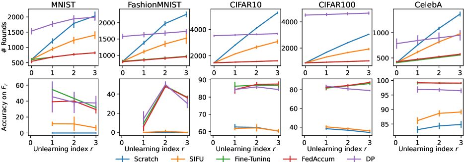
Figure 2: Total amount of aggregation rounds (1^st row) and model accuracy of unlearned clients (2^nd row) for MNIST, FashionMNIST, CIFAR10, CIFAR100, and CelebA (the lower the better). The server runs a federated routine with $M=100$ clients, and unlearns 10 of them at each unlearning request ($R=3$). Results are reported with variability estimated on 10 seeds.

In this section, we experimentally demonstrate the effectiveness of SIFU through a series of experiments introduced in Section 5.1. In Section 5.2, we illustrate and discuss our experimental results. Results and related code are publicly available.

5.1 Experimental Setup

Datasets. We report experiments on reduced versions of MNIST LeCun et al., (1998), FashionMNIST Xiao et al., (2017), CIFAR-10 Krizhevsky, (2009), CIFAR-100 Krizhevsky, (2009), and CelebA Liu et al., (2015). For each dataset, we consider $M=100$ clients, with 100 data points each. For MNIST and FashionMNIST, each client has data samples from only one class, so that each class is represented in 10 clients only. For CIFAR10 and CIFAR100, each client has data samples with ratio sampled from a Dirichlet distribution with parameter 0.1 Harry Hsu et al., (2019). Finally, in CelebA, clients own data samples representing the same celebrity as done in LEAF Caldas et al., (2018). With these five datasets, we consider different levels of heterogeneity based on label and feature distribution.

Models. For MNIST, we train a logistic regression model to consider a convex classification problem, while for the other dataset, we train a neural network with convolutional layers followed by fully connected ones. More details on the networks are available in Appendix D.

Unlearning schemes. We compare a variety of state-of-the-art FU schemes. First, we consider our proposed method SIFU as described in Algorithm 3 and set $B=1$, which is empirically-backed in Appendix E. In addition to SIFU, we consider the following unlearning schemes from the state-of-the-art: Scratch, where retraining of a new initial model is performed on the remaining clients; Fine-Tuning, where retraining is performed on the current global model with the remaining clients; Last Neel et al., (2021), where retraining is performed on the remaining clients via perturbation of the final FL global model; DP Dwork and Roth, (2014), where training with every client is performed with differential privacy, and FedAccum Liu et al., (2021), where retraining is performed on the current global model from which the server removes the updates of the clients to unlearn, by re-aggregating the parameter updates of clients that were stored by the server across FL iterations. We remind that FedAccum does not provide quantitative guarantees of the unlearning procedure, and requires the server to store the full sequence of models during the FL procedure.

Experimental scenario. We consider a sequential unlearning scenario in which the server performs FL training and then receives $R=3$ sequential unlearning requests to unlearn 10 random clients per request. In the special case of MNIST and FashionMNIST, the server must unlearn 10 clients owning the same class. The server orchestrates each unlearning scheme through retraining until the global model accuracy on the remaining clients exceeds a fixed threshold specific to each dataset. The stopping accuracies considered are 93% for MNIST, 90% for FashionMNIST, CIFAR10, and CIFAR100, and 99.9% for CelebA. We set the minimum number of 50 aggregation rounds, and a maximum budget of 10000 rounds when the stopping accuracy threshold is not reached. Hence, the maximum accuracy of a model is equal to the prescribed threshold. Each unlearning method is applied with same hyperparameters, i.e. stopping accuracy, local learning rate $\eta$, and amount of SGD steps $K$ (Appendix D). We define the set of clients requesting unlearning as:

$$F_{r}=\cup_{s=1}^{r}W_{s}.$$ (18)

In our experimental scenario, we have $|F_{0}|=0$ during training and $|F_{1}|=10$, $|F_{2}|=20$, and $|F_{3}|=30$ after each unlearning request.

Unlearning quantification. We verify the success of an unlearning scheme with two metrics: (a) the amount of server aggregation rounds needed for retraining, and (b) the resulting model accuracy on the unlearned clients. We note that, by construction, Scratch provides perfect unlearning of the clients from a request $W_{r}$. Therefore, we consider an unlearning scheme successful if it reaches similar accuracy of Scratch with less aggregation rounds, when tested on the data samples of $F_{r}$.

5.2 Experimental Results

Figure 2 shows that for every dataset and unlearning index, Fine-Tuning, FedAccum, and DP provide similar model accuracy for the unlearned clients in $F_{r}$ (Figure 2-2^nd row), albeit significantly higher than for Scratch, the unlearning standard. Noteworthy, unlearning with Fine-Tuning, FedAccum results in significantly less aggregation rounds than Scratch (Figure 2-1^st row). We note that SIFU and Scratch lead to similar unlearning results, quantified by low accuracy on the unlearned clients $F_{r}$ (Figure 2-2^nd row), while SIFU unlearns these clients in roughly half the amount of aggregation rounds needed for Scratch (Figure 2-1^st row). However, the model accuracy of SIFU is slightly higher than the one of Scratch, with perfect overlap only for FashionMNIST. This behavior is natural and can be explained by our privacy budget $(\epsilon,\delta)$, which trades unlearning capabilities for effectiveness of the retraining procedure. With highest unlearning budget, i.e. $\epsilon=1$ and $\delta=0$, SIFU would require to retrain from the initial model ${\bm{\theta}}_{0}^{0}$, thus reducing to Scratch. The poor unlearning performance of DP can be explained by the fact that it provides privacy guarantees with respect to every client, while FU only aims at removing the contribution of a few specific clients.

Finally, we observed that when unlearning with Last, the retrained model always converged to a local optimum with accuracy inferior to our target after $10^{3}$ aggregation rounds. This behavior is likely due to the difficulty of calibrating the noise perturbation with heterogeneous contributions of the clients. For this reason, we decided to exclude Last from the plots of Figure 2.

5.3 Verifying Unlearning through Watermarking

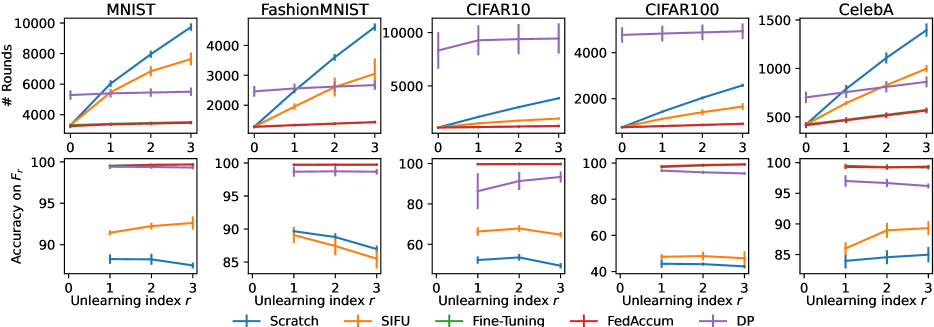
Figure 3: Total amount of aggregation rounds (1^st row) and model accuracy of unlearned clients (2^nd row) for the unlearning of watermarked data from MNIST, FashionMNIST, CIFAR10, CIFAR100, and CelebA (the lower the better).

The work of Sommer et al., (2020) proposes an adversarial approach to verify the unlearning efficiency through watermarking. We apply this method to our federated setting, in which watermarking is operated by each client by randomly assigning the maximum possible value to 10 given pixels of each data sample. To ensure that clients’ heterogeneity is only due to the modification of the pixels, we define data partitioning across clients by randomly assigning the data according to a Dirichlet distribution with parameter 1. Figure 3 in Appendix D shows our results for this experimental scenario on every dataset. We retrieve the same conclusions drawn from Figure 2. SIFU and Scratch have similar accuracies on the unlearned clients in $F_{r}$, which demonstrate the effectiveness of the unlearning. Moreover, SIFU unlearns these clients in significantly less aggregation rounds than Scratch.

5.4 Impact of the noise perturbation on SIFU

Appendix D illustrates the impact of the perturbation amplitude $\sigma$ on convergence speed when unlearning with SIFU. We note that when unlearning with a small $\sigma$, SIFU has identical behavior to Scratch as the unlearning is applied to the initial random model ${\bm{\theta}}_{0}^{0}$. With large values of $\sigma$, SIFU performs instead identically to Last and applies the unlearning to the final global model ${\bm{\theta}}_{r}^{N_{r}}$.

6 Conclusions

In this work, we introduce IFU, a general federated unlearning scheme to unlearn a client’s contribution from a model trained with FL. Upon receiving an unlearning request from a given client, IFU identifies the optimal FL iteration from which to re-initialise the optimisation. IFU allows scalability with respect to the model size and FL iterations, and generalizes beyond the convex assumption on the clients loss functions. We further extend the theory of IFU to account for the practical scenario of SIFU, where the server receives series of unlearning requests from multiple clients. We prove that SIFU accounts for sequences of requests while satisfying the unlearning guarantees.

An additional contribution of this work consists in a new theory for bounding the clients contribution in FL, which can be computed for every client without additional computation or communication. The theoretical framework of SIFU only assumes that clients’ loss functions are smooth without relying on the following strong assumptions typical of the MU literature: strong convexity of the clients’ loss functions, approximation of the clients’ gradients, and computation/approximation of the client’s Hessian. The relevance of our approach is also experimentally verified on both convex and non-convex problems across several benchmarks.

Appendix A When fine tuning does not guarantee unlearning: example on linear regression

Let us consider a linear regression optimization, with feature matrix ${\bm{X}}$ and predictions ${\bm{y}}$ such that the loss function $f$ is defined as

$$f({\bm{X}},{\bm{y}},{\bm{\theta}})=\frac{1}{2}\left[{\bm{y}}-{\bm{X}}{\bm{\theta}}\right]^{T}\left[{\bm{y}}-{\bm{X}}{\bm{\theta}}\right].$$ (19)

In this example, we assume there are more features than data samples, which makes ${\bm{X}}^{T}{\bm{X}}$ a singular matrix. While $f$ is convex, $f$ has more than one global optimum. Any model with parameter ${\bm{\theta}}^{*}$ such that

$${\bm{X}}^{T}{\bm{X}}{\bm{\theta}}^{*}={\bm{X}}^{T}{\bm{y}}$$ (20)

is a global optimum. When ${\bm{X}}^{T}{\bm{X}}$ is non-singular, we retrieve the unique optimum in close-form ${\bm{\theta}}^{*}=\left({\bm{X}}^{T}{\bm{X}}\right)^{-1}{\bm{X}}^{T}{\bm{y}}$. We show with this simple example that, upon unlearning a data sample, no amount of fine-tuning on the model ${\bm{\theta}}^{*}$ can lead to the same model obtained when retraining from a random initial model. We differentiate between $({\bm{X}},{\bm{y}})$ and $({\bm{X}}_{-1},{\bm{y}}_{-1})$ our data with and without a given data point.

Optimizing $f$, as defined in equation (19), with $N$ steps of gradient descent, learning rate $\eta$, and initial model ${\bm{\theta}}_{0}$ gives model parameters ${\bm{\theta}}^{N}$ defined as

$${\bm{\theta}}^{N}=\underbrace{\left[I-\eta{\bm{X}}^{T}{\bm{X}}\right]^{N}}_{A({\bm{X}},N)}{\bm{\theta}}^{0}+\underbrace{\eta\sum_{n=0}^{N-1}\left[I-\eta{\bm{X}}^{T}{\bm{X}}\right]^{n}{\bm{X}}^{T}{\bm{y}}}_{B({\bm{X}},{\bm{y}},N)}.$$ (21)

We first note that we retrieve the standard form for the global optimum of linear regression when ${\bm{X}}^{T}{\bm{X}}$ is non-singular as $\lim_{n\to\infty}A({\bm{X}},n)=0$ and $\lim_{n\to\infty}B({\bm{X}},{\bm{y}},n)=\left({\bm{X}}^{T}{\bm{X}}\right)^{-1}{\bm{X}}^{T}{\bm{y}}$. In the general form accounting for the singular case, at least one eigenvalue of $A({\bm{X}},N)$ is equal to 1 independently from the amount of gradient descent steps $N$. Hence, the parameters of the model obtained with gradient descent optimization always depend from the ones of the initial model ${\bm{\theta}}^{0}$. Hence, when unlearning our data sample from ${\bm{\theta}}^{N}$, the resulting trained model still depends of that data samples. Indeed, if we compare the model ${\bm{\theta}}_{-1}^{\tilde{N}}$ trained on the data samples $({\bm{X}}_{-1},{\bm{y}}_{-1})$, to the model $\phi_{-1}^{\tilde{N}}$ obtained after fine-tuning the model ${\bm{\theta}}^{N}$ with $\tilde{N}$ server aggregations, we have

$$\phi_{-1}^{\tilde{N}}-{\bm{\theta}}_{-1}^{\tilde{N}}=A({\bm{X}}_{-1},\tilde{N})A({\bm{X}},N){\bm{\theta}}^{0}+A({\bm{X}}_{-1},\tilde{N})B({\bm{X}},{\bm{y}},N).$$ (22)

Appendix B Forgetting a Single Client with IFU, Theorem 1

In this section, we provide the proof of Theorem 1 and derive 3 different results when considering 3 different sets of assumptions: $f$ is smooth, $f$ is smooth and convex, and $f$ is smooth and strongly-convex.

B.1 Definitions

We define by ${\bm{\theta}}^{N}=\textsc{FedAvg}(I,N)$ and ${\bm{\phi}}^{N}=\textsc{FedAvg}(I_{-c},N)$ the models trained with FedAvg initialized at ${\bm{\theta}}_{0}$ with respectively all the clients, i.e. $I$, and all the clients but client $c$, i.e. $I_{-c}$, performing $K$ GD steps.

When clients perform $K=1$ GD steps, two consecutive global models can be related, when training with clients in $I$ as a simple GD step, i.e.

$${\bm{\theta}}^{n+1}={\bm{\theta}}^{n}-\eta\nabla f_{I}({\bm{\theta}}^{n}).$$ (23)

Let us define the gradient step operator for function $f$ at learning rate $\eta$:

$$G(f,\eta,{\bm{\theta}})={\bm{\theta}}-\eta\nabla f({\bm{\theta}})$$

B.2 General case

B.2.1 Main observation

The following results use Lemma 3.7 of Hardt et al., (2016) under its 3 possible hypothesis. Let us first notice that, with $K=1$ and without any hypothesis on $f$ besides its differentiability, we have:

$$\begin{split}\phi^{n+1}-\theta^{n+1}&=\phi^{n}-\theta^{n}-\eta[\nabla f_{I\setminus\{c\}}(\phi^{n})\\ &\hphantom{aa}-\nabla f_{I\setminus\{c\}}(\theta^{n})+\nabla f_{I\setminus\{c\}}(\theta^{n})-\nabla f_{I}(\theta^{n})]\\ &=G(f_{I\setminus\{c\}},\eta,\phi^{n})-G(f_{I\setminus\{c\}},\eta,\theta^{n})\\ &\hphantom{aa}+\eta(\nabla f_{I\setminus\{c\}}(\theta^{n})-\nabla f_{I}(\theta^{n}))\\ \end{split}$$

Then, depending on the assumptions made on $f$, we get 3 different results, all taking the same form:

$$\lVert\phi^{n+1}-\theta^{n+1}\rVert\leq B(f,\eta)\lVert\phi^{n}-\theta^{n}\rVert+\eta\lVert\nabla f_{I\setminus\{c\}}(\theta^{n})-\nabla f_{I}(\theta^{n})\rVert$$ (24)

Where we consider 3 distinct cases, each with their respective assumptions and definition of $B$:

1. If $f_{i}$ is $\beta$-smooth for every $i\in I$, then

   $$B(f_{I},\eta)=1+\eta.\beta$$ (25)

2. If $f_{i}$ is $\beta$-smooth and convex for every $i\in I$ and $\eta\leq 2/\beta$, then

   $$B(f,\eta)=1$$ (26)

3. If $f_{i}$ is $\beta$-smooth and $\mu$-strongly-convex for every $i\in I$ and $\eta\leq\frac{2}{\beta+\mu}$, then

   $$B(f,\eta)=1-\frac{\eta\beta\mu}{\beta+\mu}$$ (27)

B.2.2 Generic proof

Let us prove the desired results with a generic function $B$. The specific results in the 3 different cases will then be derived directly by specifying $B$ depending on the hypothesis.

Let $p_{i}=\frac{N_{i}}{N_{I}}$ and $q_{i}=\frac{p_{i}}{1-p_{c}}\cdot(1-\mathbbm{1}_{c}(i))$. Then,

$$\lVert\phi^{n+1}-\theta^{n+1}\rVert =\Big{\lVert}\sum\limits_{i=1}^{M}q_{i}\phi_{i}^{n+1}-\sum\limits_{i=1}^{M}p_{i}\theta_{i}^{n+1}\Big{\rVert}$$

$$=\Big{\lVert}\sum\limits_{i=1}^{M}q_{i}(\phi_{i}^{n+1}-\theta_{i}^{n+1})$$

$$\hphantom{aa}+\underbrace{\sum\limits_{i=1}^{M}q_{i}(\theta_{i}^{n+1}-\theta^{n})-\sum\limits_{i=1}^{M}p_{i}(\theta_{i}^{n+1}-\theta^{n})}_{\Delta_{c}(I,\theta^{n})}$$

$$\leq\sum\limits_{i=1}^{M}q_{i}\lVert\phi_{i}^{n+1}-\theta_{i}^{n+1}\rVert+\Delta_{c}(I,\theta^{n})$$

$$\leq\max_{i\in I}\lVert\phi_{i}^{n+1}-\theta_{i}^{n+1}\rVert+\Delta_{c}(I,\theta^{n})$$

where the last inequality follows from the fact that $\sum q_{i}=1$.

Now, for any $i\in I$, let us give an upper bound for $\lVert\phi_{i}^{n+1}-\theta_{i}^{n+1}\rVert$:

$$\lVert\phi_{i}^{n,k+1}-\theta_{i}^{n,k+1}\rVert =\lVert G(f_{\{i\}},\eta,\phi_{i}^{n,k})-G(f_{\{i\}},\eta,\theta_{i}^{n,k})\rVert$$ (28)

$$\leq B(f,\eta)\cdot\lVert\phi_{i}^{n,k}-\theta_{i}^{n,k}\rVert$$

where the last inequality follows from the contractivity of one step of gradient descent (see Lemma 3.7 of Hardt et al., (2016) for all 3 cases). By applying this equation recursively $K$ times, we get

$$\lVert\phi_{i}^{n+1}-\theta_{i}^{n+1}\rVert\leq B(f,\eta)^{K}\cdot\lVert\phi_{i}^{n}-\theta_{i}^{n}\rVert$$ (29)

From Eq. (28) and Eq. (29), we get:

$$\lVert\phi^{n+1}-\theta^{n+1}\rVert\leq B(f,\eta)^{K}\cdot\lVert\phi^{n}-\theta^{n}\rVert+\Delta_{c}(I,\theta^{n})$$ (30)

Now, let us prove via recurrence that:

$$\lVert\phi^{n}-\theta^{n}\rVert\leq\sum\limits_{p=0}^{n-1}B(f,\eta)^{(n-p-1)K}\cdot\Delta_{c}(I,\theta^{p})$$ (31)

The initialization is trivial since $\phi^{0}=\theta^{0}$.

We provide the proof of the recurring property in equation (32), thus verifying equation (31) and proving Theorem 1.

$$\lVert\phi^{n+1}-\theta^{n+1}\rVert \leq B(f,\eta)^{K}\Biggr{[}\sum\limits_{p=0}^{n-1}B(f,\eta)^{(n-p-1)K}\Delta_{c}(I,\theta^{p})\Biggr{]}$$ (32)

$$\quad+\Delta_{c}(I,\theta^{n})$$

$$\leq\sum\limits_{p=0}^{(n+1)-1}B(f,\eta)^{(n+1-p-1)K}\cdot\Delta_{c}(I,\theta^{p})$$

Let us now give the specific formulations for each set of assumptions.

B.3 Case $f$ smooth, not necessarily convex

Let $f$ be $\beta$-smooth. In this case, the result from Eq. (31) applies with $B$ as described in Eq. (25). Therefore:

$$\lVert\phi^{n}-\theta^{n}\rVert\leq\sum\limits_{p=0}^{n-1}(1+\eta\beta)^{(n-p-1)K}\cdot\Delta_{c}(I,\theta^{p})$$ (33)

B.4 Case $f$ smooth $\And$ convex

Let $f$ be convex and $\beta$-smooth, let $\eta\leq\frac{2}{\beta}$. In this case, the result from Eq. (31) applies with $B$ as described in Eq. (26). Therefore:

$$\lVert\phi^{n}-\theta^{n}\rVert\leq\sum\limits_{p=0}^{n-1}\Delta_{c}(I,\theta^{p})$$ (34)

B.5 Case $f$ smooth $\And$ strongly convex

Let $f$ be $\mu$-strongly convex and $\beta$-smooth, let $\eta\leq\frac{2}{\beta+\mu}$. In this case, the result from Eq. (31) applies with $B$ as described in Eq. (27). Therefore:

$$\lVert\phi^{n}-\theta^{n}\rVert\leq\sum\limits_{p=0}^{n-1}(1-\frac{\eta\beta\mu}{\beta+\mu})^{(n-p-1)K}\cdot\Delta_{c}(I,\theta^{p})$$ (35)

Appendix C Convergence of SIFU, Theorem 3

C.1 Proof of Theorem 3

Proof.

We prove by induction that ${\bm{\theta}}_{r+1}^{0}$ $(\epsilon,\delta)$-unlearns every client in $F_{r+1}=\cup_{s=1}^{r+1}W_{s}=F_{r}\cup W_{r+1}$. The initialization ($r=1$) directly follows from IFU, Algorithm LABEL:alg:unlearning_ours, with Theorem 2. With reference to equation (15), we now assume that for every unlearning request $u\leq r$, the perturbed model ${\bm{\theta}}_{u}^{0}$ $(\epsilon,\delta)$-unlearns every client in $F_{u}$, and prove that ${\bm{\theta}}_{r+1}^{0}$ $(\epsilon,\delta)$-unlearns every client in $F_{r+1}$.

• Case 1: $\forall u\leq r$, $n_{u}\leq n_{r+1}$. The model ${\bm{\theta}}_{\zeta_{r+1}}^{T_{r+1}}=H(r)[n_{r+1}]$ appears later in the training history than models ${\bm{\theta}}_{\zeta_{u}}^{T_{u}}$ and, thanks to the induction property, provides $(\epsilon,\delta)$-unlearning of every client in $F_{r}$. Thus, the model ${\bm{\theta}}_{r+1}^{0}$ guarantees the unlearning of every client in $F_{r+1}$.

• Case 2: $\exists\text{ unlearning request }u^{*}\leq r\text{ such that }n_{r+1}<n_{u*}$. By construction of the training history, the sequence $H(u^{*})$ contains the model ${\bm{\theta}}_{\zeta_{r+1}}^{T_{r+1}}=H(u^{*})[n_{r+1}]=H(r)[n_{r+1}]$, which appears earlier than model ${\bm{\theta}}_{\zeta_{u^{*}}}^{T_{u*}}=H(u^{*})[n_{u^{*}}]$. Perturbing the model ${\bm{\theta}}_{\zeta_{r+1}}^{T_{r+1}}$ with noise $N(\mathbf{0},\sigma{\bm{I}}_{\bm{\theta}}$), guarantees $(\epsilon,\delta)$-unlearning of the clients in $W_{u^{*}}$, since

  $$\Psi_{u^{*}}(n_{r+1},c^{*})\leq\Psi_{u^{*}}(n_{u^{*}},c^{*})\leq\Psi^{*},$$

  for every client $c^{*}$ in $W_{u*}$. By extending this reasoning to all learning requests $u$ such that $n_{r+1}<n_{u}$, and by the induction property for the remaining ones, the model ${\bm{\theta}}_{r+1}^{0}$ guarantees the unlearning of every client in $F_{r+1}$.

∎

Appendix D Experiments

For every benchmark, we consider the number of SGD steps $K$, batch size $B$, number of clients $M$, the number of sampled clients $m$, the standard deviation $\sigma$ of the noise perturbation, and the local learning rate $\eta$ given in Table 1. Also, for our unlearning scheme SIFU, DP, and Last, we consider an unlearning budget of $\epsilon=10$ and $\delta=0.01$. The unlearning budget plays the important role of identifying in the training history the global model to perturb. Theorem 2 shows that $\epsilon$ and $\sigma$ are linearly related. Hence, to unlearn a client $c$ from a global model $c$, a smaller $\sigma$ can be considered, but at the cost of a lower unlearning budget $(\epsilon,\delta)$, Definition 1. Also, for fair comparison of DP with other FU schemes, we select the best clipping value $C$, in a range from 0.001 to 1, for which the global model reaches the target accuracy in the smallest amount of aggregation rounds. Finally, for FashionMNIST, CIFAR10, CIFAR100, and CelebA, we consider model architectures composed of three convolutional layers followed by two fully connected layers, with implementation at [URL hidden for double-blind submission].

Table 1: Hyperparameters used for our different unlearning benchmarks described in Section 5.1.

Dataset	$K$	$B$	$M$	$m$	$\sigma$	$\eta$	$C$
MNIST	10	100	100	10	0.05	0.01	0.5
FashionMNIST	5	20	100	10	0.1	0.02	0.5
CIFAR10	5	20	100	5	0.05	0.01	0.2
CIFAR100	5	20	100	5	0.05	0.02	0.2
CelebA	10	20	100	20	0.1	0.01	0.5

The training and retraining depends on the initial model ${\bm{\theta}}_{0}^{0}$ and the clients’ batches of data used at every aggregation to compute their local SGDs. Hence, we replicate each unlearning scenario on 10 different seeds and plot in Figure 2 to 5 their averaged results. For the unlearning benchmarks described in Section 5.1 and used in Figure 2, 4, and 5, the stopping accuracies considered are 93% for MNIST, 90% for FashionMNIST, CIFAR10, and CIFAR100, and 99.9% for CelebA.

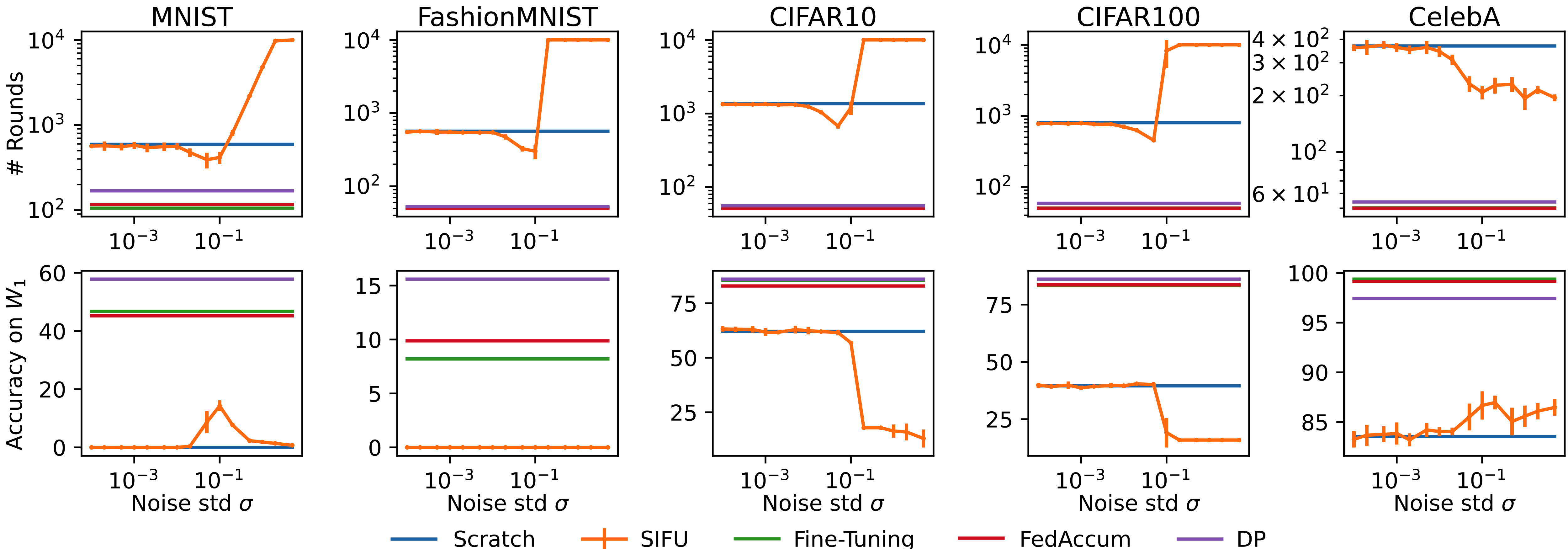
Figure 4: Impact of the noise standard deviation $\sigma$ when unlearning with SIFU for the unlearning budget $(\epsilon,\delta)=(10,0.01)$. Total amount of aggregation rounds (1^st row) and model accuracy of unlearned clients (2^nd row) for MNIST, FashionMNIST, CIFAR10, CIFAR100, and CelebA (the lower the better). We compare SIFU with Scratch, Fine-Tuning, FedAccum, and DP by reporting their total amount of aggregation rounds or model accuracy of unlearned clients. However, only SIFU depends on the value of $\sigma$, which leads to horizontal lines for the other schemes.

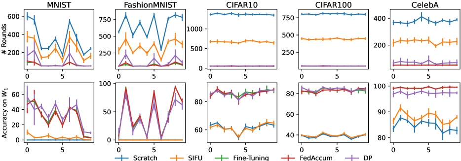
Figure 5: Total amount of aggregation rounds (1^st row) and model accuracy of unlearned clients (2^nd row) for MNIST, FashionMNIST, CIFAR10, CIFAR100, and CelebA (the lower the better). This figure displays the unlearning capabilities of the unlearning benchmarks introduced in Section 5.1 after training on clients in $I$ and unlearning $|W_{1}|=10$ clients. For each integer on the x-axis, a different set of clients to unlearn is considered. Each unlearning request is composed of 10 random clients for CIFAR10, CIFAR100, and CelebA. For MNIST and FashionMNIST, each unlearning request $|W_{1}|$ has 10 clients of the same class such that the x-axis is the class forgotten. The integers on the x-axis corresponds to the class of the clients to unlearn.

Appendix E Bound from theorem 1

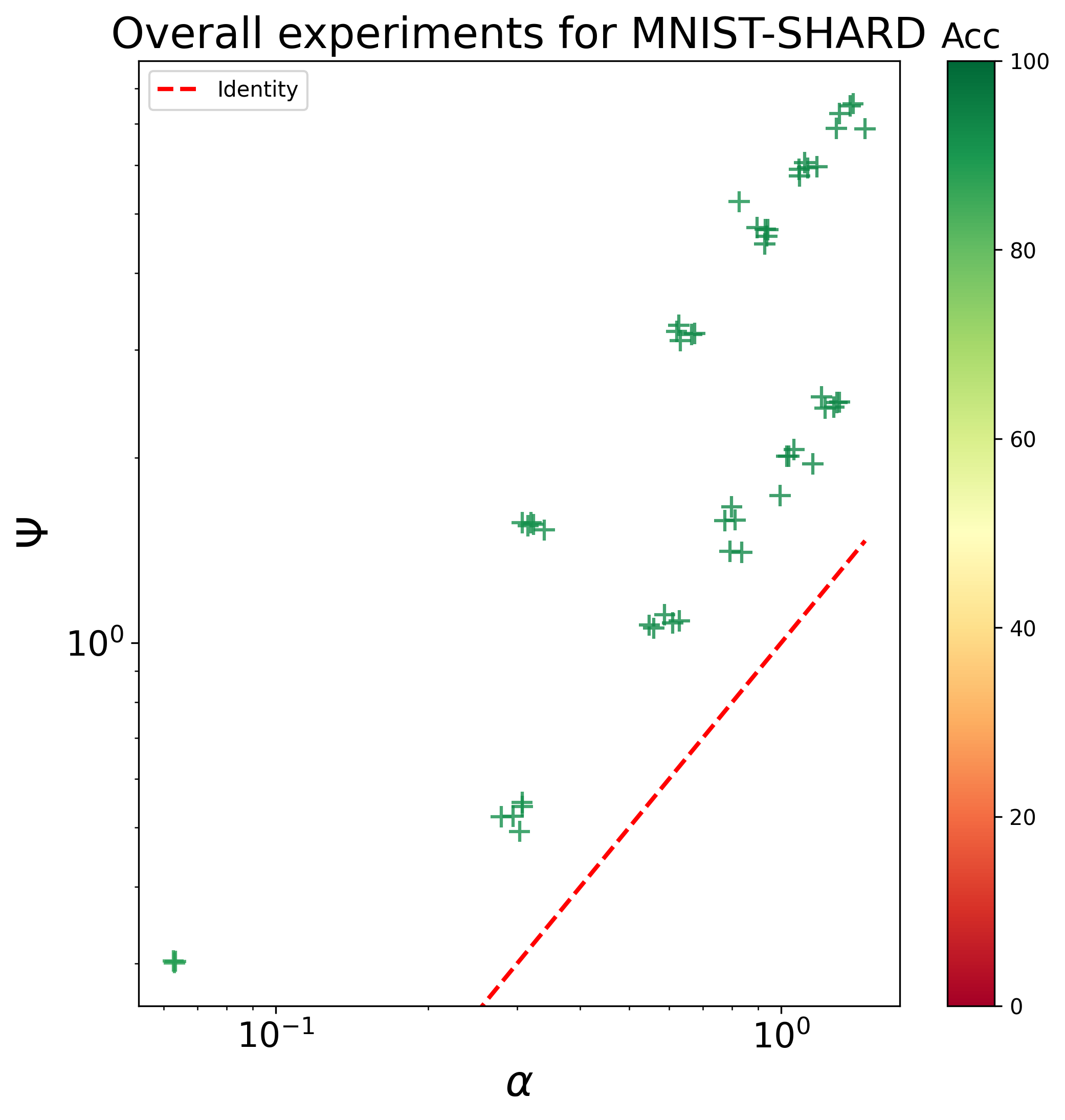
(a) MNIST-shard dataset

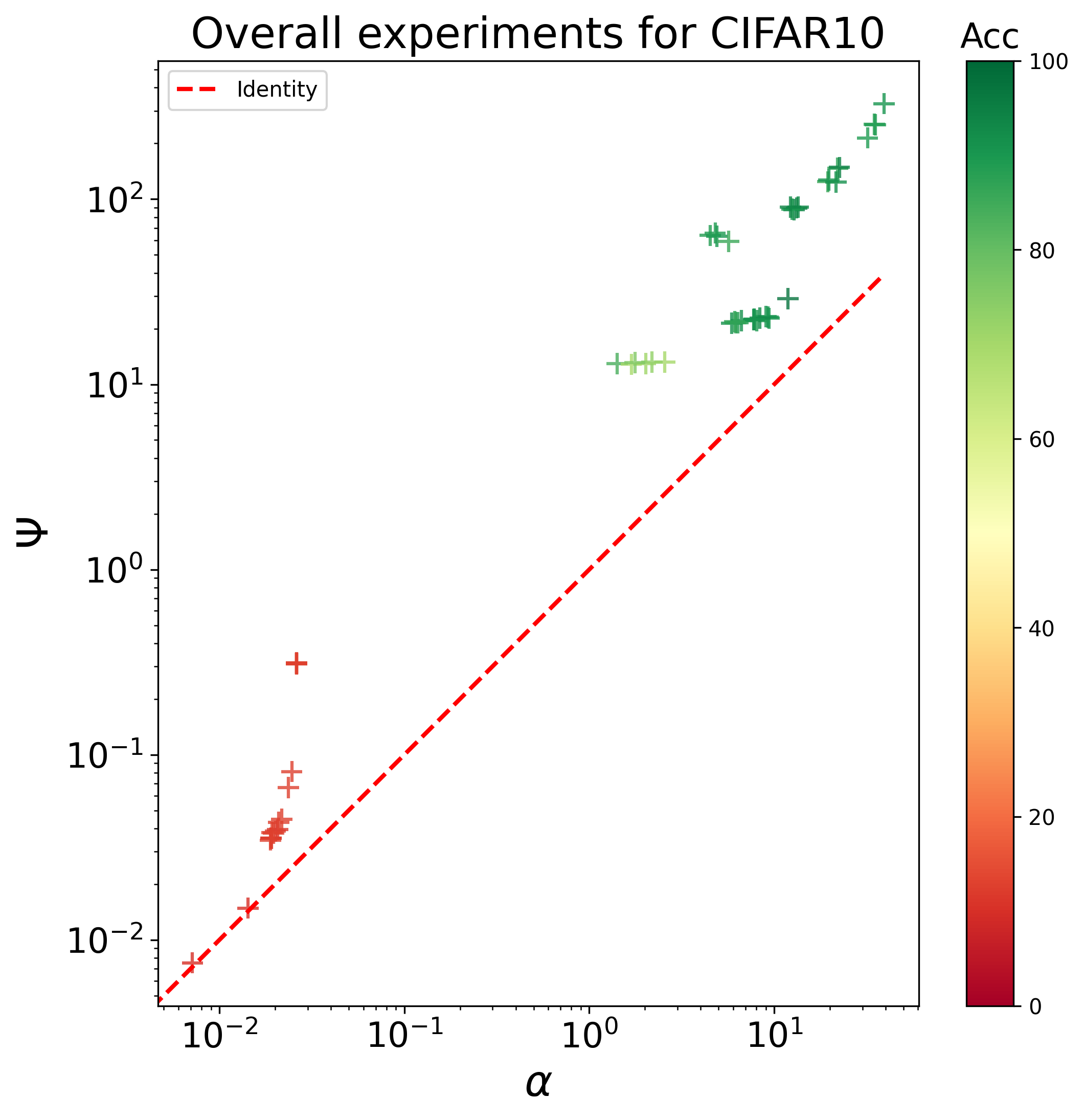
(b) CIFAR10 dataset

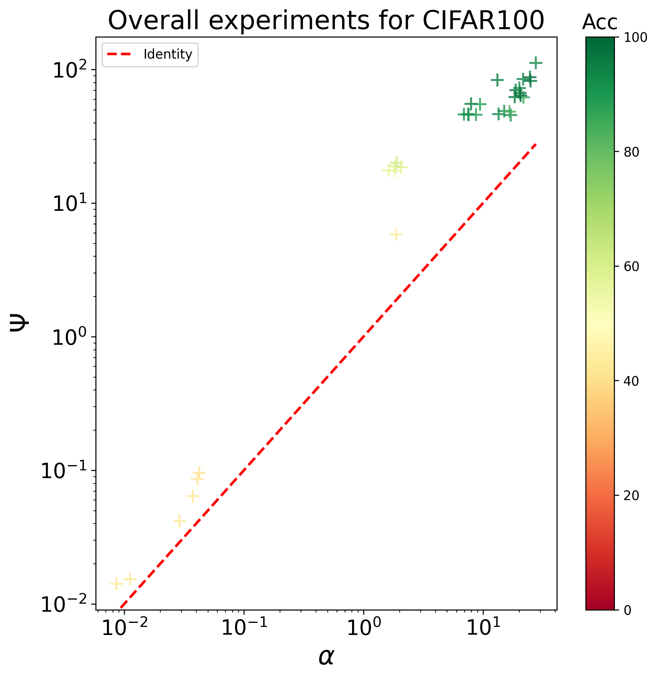
(c) CIFAR100 dataset

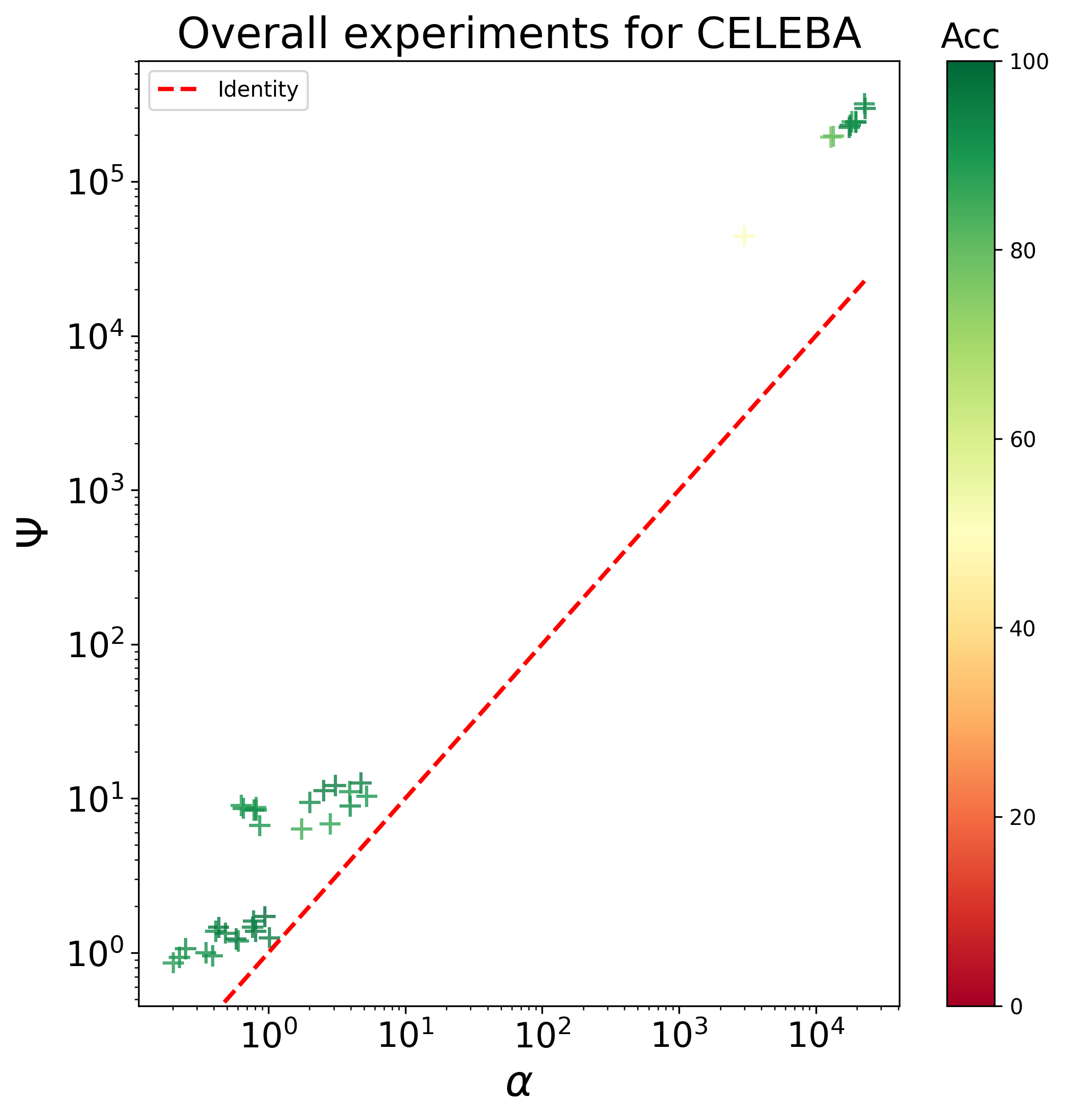
(d) CELEBA dataset

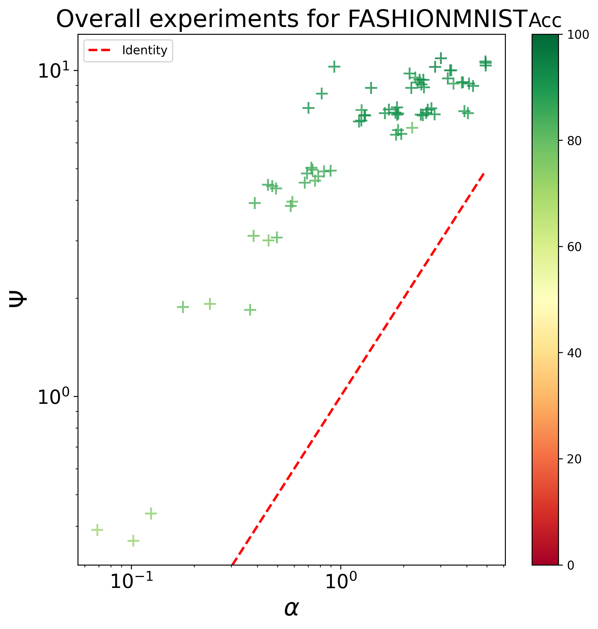
(a) FashionMNIST dataset

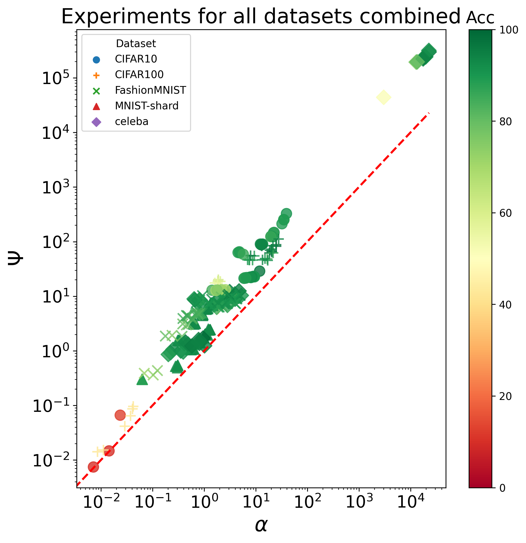
(b) All datasets

Figure 7: Comparison between $\Psi$ and $\alpha$ for $B=1$ for all datasets and various hyper-parameters.

To investigate whether it is legitimate to pick $B(f,\eta)=1$ for our experiments, we empirically measure $\alpha$ and $\Psi$ for all our datasets with a large set of hyper-parameter choices, ranging from the ones used in the experiments to less adapted ones, even included some that do not allow convergence. The bound from Theorem 1 holds for every experimental scenario we tried. The results are displayed in figure 7.

References

- Abadi et al., (2016) Abadi, M., Chu, A., Goodfellow, I., McMahan, H. B., Mironov, I., Talwar, K., and Zhang, L. (2016). Deep learning with differential privacy. In Proceedings of the 2016 ACM SIGSAC conference on computer and communications security, pages 308–318.
- Bourtoule et al., (2021) Bourtoule, L., Chandrasekaran, V., Choquette-Choo, C. A., Jia, H., Travers, A., Zhang, B., Lie, D., and Papernot, N. (2021). Machine unlearning. In 2021 IEEE Symposium on Security and Privacy (SP), pages 141–159. IEEE.
- Caldas et al., (2018) Caldas, S., Duddu, S. M. K., Wu, P., Li, T., Konečný, J., McMahan, H. B., Smith, V., and Talwalkar, A. (2018). LEAF: A Benchmark for Federated Settings. NeurIPS.
- Cao and Yang, (2015) Cao, Y. and Yang, J. (2015). Towards making systems forget with machine unlearning. 2015 IEEE Symposium on Security and Privacy, pages 463–480.
- Chen et al., (2020) Chen, X., Wu, S. Z., and Hong, M. (2020). Understanding gradient clipping in private sgd: A geometric perspective. In Larochelle, H., Ranzato, M., Hadsell, R., Balcan, M., and Lin, H., editors, Advances in Neural Information Processing Systems, volume 33, pages 13773–13782. Curran Associates, Inc.
- Dwork and Roth, (2014) Dwork, C. and Roth, A. (2014). The algorithmic foundations of differential privacy. Found. Trends Theor. Comput. Sci., 9(3–4):211–407.
- Fredrikson et al., (2015) Fredrikson, M., Jha, S., and Ristenpart, T. (2015). Model inversion attacks that exploit confidence information and basic countermeasures. In Proceedings of the 22nd ACM SIGSAC Conference on Computer and Communications Security, CCS ’15, page 1322–1333, New York, NY, USA. Association for Computing Machinery.
- Ginart et al., (2019) Ginart, A., Guan, M., Valiant, G., and Zou, J. Y. (2019). Making ai forget you: Data deletion in machine learning. In Wallach, H., Larochelle, H., Beygelzimer, A., d'Alché-Buc, F., Fox, E., and Garnett, R., editors, Advances in Neural Information Processing Systems, volume 32. Curran Associates, Inc.
- Golatkar et al., (2021) Golatkar, A., Achille, A., Ravichandran, A., Polito, M., and Soatto, S. (2021). Mixed-privacy forgetting in deep networks. In Proceedings of the IEEE/CVF Conference on Computer Vision and Pattern Recognition (CVPR), pages 792–801.
- (10) Golatkar, A., Achille, A., and Soatto, S. (2020a). Eternal sunshine of the spotless net: Selective forgetting in deep networks. In Proceedings of the IEEE/CVF Conference on Computer Vision and Pattern Recognition (CVPR).
- (11) Golatkar, A., Achille, A., and Soatto, S. (2020b). Forgetting outside the box: Scrubbing deep networks of information accessible from input-output observations.
- Guo et al., (2020) Guo, C., Goldstein, T., Hannun, A., and Van Der Maaten, L. (2020). Certified data removal from machine learning models. In III, H. D. and Singh, A., editors, Proceedings of the 37th International Conference on Machine Learning, volume 119 of Proceedings of Machine Learning Research, pages 3832–3842. PMLR.
- Gupta et al., (2021) Gupta, V., Jung, C., Neel, S., Roth, A., Sharifi-Malvajerdi, S., and Waites, C. (2021). Adaptive machine unlearning. In Ranzato, M., Beygelzimer, A., Nguyen, K., Liang, P. S., Vaughan, J. W., and Dauphin, Y., editors, Advances in Neural Information Processing Systems, volume 34, pages 16319–16330. Curran Associates, Inc.
- Halimi et al., (2022) Halimi, A., Kadhe, S., Rawat, A., and Baracaldo, N. (2022). Federated unlearning: How to efficiently erase a client in fl? arXiv preprint arXiv:2207.05521.
- Harding et al., (2019) Harding, E. L., Vanto, J. J., Clark, R., Hannah Ji, L., and Ainsworth, S. C. (2019). Understanding the scope and impact of the california consumer privacy act of 2018. Journal of Data Protection & Privacy, 2(3):234–253.
- Hardt et al., (2016) Hardt, M., Recht, B., and Singer, Y. (2016). Train faster, generalize better: Stability of stochastic gradient descent. In International conference on machine learning, pages 1225–1234. PMLR.
- Harry Hsu et al., (2019) Harry Hsu, T. M., Qi, H., and Brown, M. (2019). Measuring the effects of non-identical data distribution for federated visual classification. arXiv preprint arXiv:1909.06335.
- Izzo et al., (2021) Izzo, Z., Anne Smart, M., Chaudhuri, K., and Zou, J. (2021). Approximate data deletion from machine learning models. In Banerjee, A. and Fukumizu, K., editors, Proceedings of The 24th International Conference on Artificial Intelligence and Statistics, volume 130 of Proceedings of Machine Learning Research, pages 2008–2016. PMLR.
- Jia et al., (2023) Jia, J., Liu, J., Ram, P., Yao, Y., Liu, G., Liu, Y., Sharma, P., and Liu, S. (2023). Model sparsification can simplify machine unlearning. arXiv preprint arXiv:2304.04934.
- Jin et al., (2023) Jin, R., Chen, M., Zhang, Q., and Li, X. (2023). Forgettable federated linear learning with certified data removal. arXiv preprint arXiv:2306.02216.
- Krizhevsky, (2009) Krizhevsky, A. (2009). Learning multiple layers of features from tiny images.
- LeCun et al., (1998) LeCun, Y., Bottou, L., Bengio, Y., and Ha, P. (1998). LeNet. Proceedings of the IEEE.
- Li et al., (2020) Li, X., Huang, K., Yang, W., Wang, S., and Zhang, Z. (2020). On the convergence of fedavg on non-iid data. In International Conference on Learning Representations.
- Liu et al., (2021) Liu, G., Ma, X., Yang, Y., Wang, C., and Liu, J. (2021). Federaser: Enabling efficient client-level data removal from federated learning models. In 2021 IEEE/ACM 29th International Symposium on Quality of Service (IWQOS), pages 1–10.
- Liu et al., (2022) Liu, Y., Xu, L., Yuan, X., Wang, C., and Li, B. (2022). The right to be forgotten in federated learning: An efficient realization with rapid retraining. Proceedings - IEEE INFOCOM, 2022-May:1749–1758.
- Liu et al., (2015) Liu, Z., Luo, P., Wang, X., and Tang, X. (2015). Deep learning face attributes in the wild. In Proceedings of International Conference on Computer Vision (ICCV).
- (27) Mahadevan, A. and Mathioudakis, M. (2021a). Certifiable machine unlearning for linear models. CoRR, abs/2106.15093.
- (28) Mahadevan, A. and Mathioudakis, M. (2021b). Certifiable machine unlearning for linear models. arXiv preprint arXiv:2106.15093.
- (29) McMahan, B., Moore, E., Ramage, D., Hampson, S., and y Arcas, B. A. (2017a). Communication-Efficient Learning of Deep Networks from Decentralized Data. In Singh, A. and Zhu, J., editors, Proceedings of the 20th International Conference on Artificial Intelligence and Statistics, volume 54 of Proceedings of Machine Learning Research, pages 1273–1282, Fort Lauderdale, FL, USA. PMLR.
- McMahan et al., (2018) McMahan, H. B., Andrew, G., Erlingsson, U., Chien, S., Mironov, I., Papernot, N., and Kairouz, P. (2018). A general approach to adding differential privacy to iterative training procedures. arXiv preprint arXiv:1812.06210.
- (31) McMahan, H. B., Ramage, D., Talwar, K., and Zhang, L. (2017b). Learning differentially private recurrent language models. arXiv preprint arXiv:1710.06963.
- Neel et al., (2021) Neel, S., Roth, A., and Sharifi-Malvajerdi, S. (2021). Descent-to-delete: Gradient-based methods for machine unlearning. In Feldman, V., Ligett, K., and Sabato, S., editors, Proceedings of the 32nd International Conference on Algorithmic Learning Theory, volume 132 of Proceedings of Machine Learning Research, pages 931–962. PMLR.
- Pan et al., (2022) Pan, C., Sima, J., Prakash, S., Rana, V., and Milenkovic, O. (2022). Machine unlearning of federated clusters. arXiv preprint arXiv:2210.16424.
- Sommer et al., (2020) Sommer, D. M., Song, L., Wagh, S., and Mittal, P. (2020). Towards probabilistic verification of machine unlearning. arXiv preprint arXiv:2003.04247, abs/2003.04247.
- Voigt and Von dem Bussche, (2017) Voigt, P. and Von dem Bussche, A. (2017). The eu general data protection regulation (gdpr). A Practical Guide, 1st Ed., Cham: Springer International Publishing, 10(3152676):10–5555.
- Wang et al., (2021) Wang, J., Guo, S., Xie, X., and Qi, H. (2021). Federated unlearning via class-discriminative pruning.
- Wang et al., (2020) Wang, J., Liu, Q., Liang, H., Joshi, G., and Poor, H. V. (2020). Tackling the objective inconsistency problem in heterogeneous federated optimization. In Larochelle, H., Ranzato, M., Hadsell, R., Balcan, M., and Lin, H., editors, Advances in Neural Information Processing Systems 33: Annual Conference on Neural Information Processing Systems 2020, NeurIPS 2020, December 6-12, 2020, virtual.
- Wu et al., (2022) Wu, C., Zhu, S., and Mitra, P. (2022). Federated unlearning with knowledge distillation. arXiv preprint arXiv:2201.09441.
- Xiao et al., (2017) Xiao, H., Rasul, K., and Vollgraf, R. (2017). Fashion-mnist: a novel image dataset for benchmarking machine learning algorithms. arXiv preprint arXiv:1708.07747, abs/1708.07747.