Plug and Play Active Learning for Object Detection

Abstract

Annotating data for supervised learning is expensive and tedious, and we want to do as little of it as possible. To make the most of a given “annotation budget” we can turn to active learning (AL) which aims to identify the most informative samples in a dataset for annotation. Active learning algorithms are typically uncertainty-based or diversity-based. Both have seen success in image classification, but fall short when it comes to object detection. We hypothesise that this is because: (1) it is difficult to quantify uncertainty for object detection as it consists of both localisation and classification, where some classes are harder to localise, and others are harder to classify; (2) it is difficult to measure similarities for diversity-based AL when images contain different numbers of objects. We propose a two-stage active learning algorithm Plug and Play Active Learning (PPAL) that overcomes these difficulties. It consists of (1) Difficulty Calibrated Uncertainty Sampling, in which we used a category-wise difficulty coefficient that takes both classification and localisation into account to re-weight object uncertainties for uncertainty-based sampling; (2) Category Conditioned Matching Similarity to compute the similarities of multi-instance images as ensembles of their instance similarities. PPAL is highly generalisable because it makes no change to model architectures or detector training pipelines. We benchmark PPAL on the MS-COCO and Pascal VOC datasets using different detector architectures and show that our method outperforms the prior state-of-the-art. Code is available at https://github.com/ChenhongyiYang/PPAL

1 Introduction

Figure 1: An overview of our two-stage PPAL. In the first stage we perform Difficulty Calibrated Uncertainty Sampling: the objects’ uncertainties are re-weighted by difficulty coefficients that take both classification and localisation into account, and a candidate pool of images with the highest uncertainty scores are sampled. In the second stage, we run a modified kmeans++ algorithm using Category Conditioned Matching Similarity to select a set of representative images as active learning queries.

Object detectors typically need a huge amount of training data [26, 21] annotated with both object category labels and bounding box locations. Annotating data is expensive and tedious. If we are required to do some annotation, it would make sense to annotate the images that will be of the greatest benefit when used for training. But how do we know which ones to choose? The goal of active learning is to tell us. Given a large unlabelled data pool, active learning (AL) aims to sample data that would maximally improve a model’s performance if that data was annotated and used for training. There are two main streams of active learning methods: (1) Uncertainty-based active learning methods [39, 23, 22, 20, 35] select samples that maximise a measure of model uncertainty e.g. those with the least mutual information with the current set of labelled data; (2) Diversity-based active learning approaches [38, 1, 29, 30, 16, 13, 44, 3, 41] instead select samples that are diverse and can represent of the whole distribution of unlabelled data; this can be achieved selecting the subset of samples for which the sample similarities are minimised.

With a neural network, uncertainty-based and diversity-based AL can be straightforwardly applied to the task of image classification. For example, uncertainty-based sampling can be implemented by selecting the unlabelled samples with maximum classification entropy. Diversity-based sampling can be achieved by computing similarities using averaged feature maps. However, designing an effective AL strategy for object detection is more challenging. This is because detection consists of both object localisation and classification. It is difficult to quantify uncertainty jointly across both tasks e.g. we may have an object that is easy to localise, but hard to classify. Also, it is hard to measure similarity when images contain multiple objects with different features. Several works have tackled AL for detection [4, 46, 10] but rely on modifying the architecture of an object detector as well as the training pipeline. This means they cannot be easily integrated into other object detector frameworks without significant engineering effort.

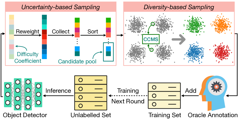
In this work we propose Plug and Play Active Learning (PPAL) for object detection. It is state-of-the-art and easy to use; it requires no modifications to architectures or training pipelines and works across a wide range of object detectors. PPAL is a two-stage algorithm that combines uncertainty- and diversity-based sampling: in the first stage it selects a candidate pool of images with high uncertainty scores from a large unlabelled dataset, then in the second stage it selects a highly diverse AL query set from this pool for annotation. In more detail, we propose Difficulty Calibrated Uncertainty Sampling (DCUS) for the first stage, in which category-wise difficulty coefficients are computed and updated during training and then used to re-weight the instance uncertainties when selecting samples. The difficulty coefficients take both classification and localisation difficulties into account, so are highly suitable for object detection. DCUS also favours the sampling of images containing objects in challenging categories, hence benefiting the overall average precision (AP). For the second stage, we propose Category Conditioned Matching Similarity (CCMS): a new method for measuring similarities for multi-instance images, in which every object is matched to its most similar counterpart in another image to compute instance-wise similarity. Image-wise similarity is then computed by ensembling instance-wise similarities. CCMS is used off-the-shelf by a modified kmeans++ algorithm to select a diverse and representative subset as the active learning queries from the pool selected in the first stage. Unlikely recently proposed work [4, 46, 10], PPAL does not modify the model architecture or training pipeline of object detectors, thus it is highly generalisable to different types of detectors. To summarise, our contributions are as follows:

• We propose PPAL, a two-stage active learning algorithm for object detection that combines uncertainty-based and diversity-based sampling. It is plug-and-play, requiring no architectural modifications or any change to training pipelines.

• We show that PPAL outperforms previous object detection AL algorithms across multiple object detectors on the COCO and Pascal VOC datasets. We also show that our method easily generalise to different object detectors and backbone networks.

2 Related Work

Active Learning. Active learning approaches can be broadly separated into uncertainty-based and diversity-based methods. Uncertainty-based methods [39, 23, 22, 20, 35] aim to select samples for annotation that maximise some uncertainty measure; common measures include entropy [39, 20] and the margin between the largest two predicted class posterior probabilities [35, 20, 11]. In [15] the model uncertainty is estimated by performing multiple forward passes with Monte Carlo Dropout. Learn Loss [45] uses a prediction of the loss as a measure of uncertainty. Diversity-based methods [38, 1, 29, 30, 16, 13, 44, 3, 41] for AL aim to select representative samples so that a small subset of data can describe the whole dataset. Core-set [38] uses a greedy k-centroid algorithm to select a small core set from the unlabelled pool and use mixed integer programming to iteratively improve sample diversity. CDAL [1] utilises predicted probabilities to improve context diversity. Recently, several works have been proposed that combine uncertainty-based and diversity-based AL. In [49, 31], k-means is performed on image features weighted by model uncertainty. In BADGE [2], a k-means++ algorithm seeding on the gradients of the model’s last layer is used to balance uncertainty and diversity. HAC [11] first clusters the unlabelled samples and queries the most uncertain samples in each cluster in a round-robin way.

Object Detection. ConvNet-based object detectors usually follow a two-stage or single-stage design. Two-stage detectors [33, 17, 5, 7] use a region proposal network [33] to extract plausible objects and the RoIAlign operation [17] to extract regional features for further classification and localisation; Single-stage [19, 32, 27, 9, 25, 40, 48, 34] detectors directly predict objects’ bounding box and category label on every position of the image feature maps. In early single-stage detectors like SSD [27], object from differet feature levels are detected using different convolutional kernels, while in the recent ones [9, 25, 40, 48] objects are detected using weight-sharing kernels. Recently, a wave of transformer-based detectors [6, 50, 24, 47] have been proposed. They use self-attention to exchange information between query vectors and image features and directly output detected objects without non-maximum-suppression.

Active Learning for Object Detection. Early attempts at applying AL to object detection [1, 38, 45] involved the direct application of image classification AL algorithms. However, these do not account for the joint classification and localisation tasks that make up detection, or the fact that images can contain multiple different objects. This prompted the design of AL algorithms specifically for detection. MDN [10] modifies an object detector to learn a Gaussian mixture model (GMM) for both the classification and regression outputs. The uncertainties of both tasks are then derived from the modelled GMMs. In [12], semi-supervised learning is used to deal with false positives and compute model uncertainty. MIAL [46] uses adversarial training to compute model discrepancy, which is used for computing uncertainty. In [42], detection scores are replaced by model uncertainties in NMS to find uncertain objects, and a set of diverse prototypes is used to select the most representative samples. However, a problem of previous works in AL for object detection is that the model architecture or training pipelines are modified to suit the AL purpose, which limits their generalisation ability across different architectures.

Algorithm 1 Pseudo-code of PPAL in Python style

⬇

# Global Parameters:

# b: per-round active learning budget

# delta: budget expanding ratio

# N: number of unlabelled images

# M: number of detected objects per image

# d: the dimension of object features

def CCMS(fs, Cs, Ss, n):

fs_1 = fs.view(n,1,M,d).expand(n,n,M,d)

Cs_1 = Cs.view(n,1,M,1).expand(n,n,M,M)

Ss_1 = Ss.view(n,1,M).expand(n,n,M)

fs_2 = fs.view(1,n,M,d).expand(n,n,M,d)

Cs_2 = Cs.view(1,n,M,1).expand(n,n,M,M)

Ss_2 = Ss.view(1,n,M).expand(n,n,M)

cos_sim = matmul(fs_1, fs_2.transpose(2,3)) + 1

diff_c = Cs_1 != Cs_2.transpose(2,3)

cos_sim[diff_c] = 0 # same class condition

sim12 = (Ss1 * cos_sim.max(dim=3)).sum(dim=2) / M

sim21 = (Ss2 * cos_sim.max(dim=2)).sum(dim=2) / M

return 0.5 * (sim12 + sim21)

def kmeansPP(sim_mat, K, init_cs):

centers = init_cs

while not converge:

center_sim = sim_mat[:, centers]

c_assign = argmax(center_sim, dim=1)

new_centers = []

for i in range(K):

clus_i = where(c_assign == i)

sim_mat_i = sim_mat[clus_i][:, clus_i]

c_i = clus_i[argmax(sim_mat_i.sum(dim=1))]

new_centers.append(c_i)

centers = new_centers

return centers

def PPAL(Fs, Cs, Ss, Us, ws)

# Fs: normalised object features, (N, M, d)

# Cs: object categories, (N, M)

# Ss: detection scores, (N, M)

# Us: object uncertainties, (N, M)

# ws: class-wise uncertainty weights in Eq.(4)

# uncertainty-based sampling

obj_ws = ws[Cs.view(-1)].view(N,M)

img_Us = (Us * obj_ws).sum(dim=1)

pInds = argsort(img_Us)[-(delta*b):]

pFs, pCs, pSs = Fs[pInds], Cs[pInds], Ss[pInds]

# diversity-based sampling

sim_mat = CCMS(pFs, pCs, pSs, pFs.size(0))

init_cs = k_center_greedy(sim_mat, b)

queries = kmeansPP(sim_mat, b, init_cs)

return queries

3 Methodology

Figure 2: An illustration of how different category-wise difficulty coefficients correspond to the evaluated detection APs for that category on Pascal VOC at each active learning round. Difficulty coefficients are sorted in descending order. Objects in categories with high-difficulty coefficients are harder to detect than those in categories with low-difficulty coefficients.

In this section we formally define the problem of active learning for object detection (Sec. 3.1) before providing an overview of our approach (Sec. 3.2). The two key innovations of our method are described in detail in Sec. 3.3 and 3.4 respectively. Figure 1 gives a high-level overview of our algorithm, and the Python-style pseudo-code is provided in Algorithm 1.

3.1 Problem Statement

We start by formally defining the problem of active learning for object detection. We follow previous work [10, 46, 42] and use a batch active learning setting, i.e. at each round we query a batch of images for oracle annotation instead of a single sample. Suppose there is a training set $X_{T}=\{x_{i}\}_{i\in[N_{t}]}$ with size $N_{t}$ and a validation set $X_{V}=\{x_{i}\}_{i\in[N_{v}]}$ with size $N_{v}$. At round $r\geq 0$, the labelled set is $X_{L}^{r}$ and the unlabelled pool is $X_{U}^{r}$ where $X_{L}^{r}\cap X_{U}^{r}=\O$ and $X_{L}^{r}\cup X_{U}^{r}=X_{T}$. An object detection model $f^{r}_{\theta}$ with parameters $\theta$ is trained on $X_{L}^{r}$ and its performance on $X_{V}$ is $Z(X_{V}|f^{r}_{\theta})$, which is usually measured by mean Averaged Precision (mAP). Given budget $b$, an active learning algorithm selects a query set $X_{Q}^{r}\subseteq X_{U}^{r}$ with size $b$ for oracle annotation. Then we can get the labelled set $X_{L}^{r+1}=X_{L}^{i}\cup X_{Q}^{r}$ and the unlabelled $X_{U}^{r+1}=X_{U}^{i}-X_{Q}^{r}$ for the next round $r+1$. Finally, the detection model is trained on $X_{L}^{r+1}$ to get $f^{r+1}_{\theta}$ with performance $Z(X_{V}|f^{r+1}_{\theta})$. After $k$ rounds of active learning, an active learning algorithm is evaluated by the model’s improvement over the initial round $\triangle Z^{k,0}=Z(X_{V}|f^{k}_{\theta})-Z(X_{V}|f^{0}_{\theta})$, i.e., the AL algorithm that can bring most performance improvement is favoured.

Figure 3: A comparison of global similarity to our proposed CCMS. The global similarity is computed using the averaged image feature maps. This fails to capture fine-grained spatial information in multi-instance images. In CCMS, each object in an image finds its most similar counterpart with the same category in another image to compute similarities. Then image-wise similarity is computed by averaging the object similarities.

3.2 Plug and Play Active Learning

Our PPAL is a two-stage active learning algorithm for object detection. In the first stage it uses Difficulty Calibrated Uncertainty Sampling (Sec. 3.3) to sample a candidate pool of images with high uncertainty scores. The second stage performs diversity-based sampling on this pool by running a kmeans++ algorithm using Category Conditioned Matching Similarity (Sec. 3.4) to select a group of representative images as active learning queries. Our algorithm can select both uncertain and diverse samples and is highly generalisable because it does not modify a detector’s model architecture or training pipeline.

3.3 Difficulty Calibrated Uncertainty Sampling

Difficulty Calibrated Uncertainty Sampling (DCUS) serves two purposes: (1) it provides a means to score uncertainty for object detection based on both classification and localisation; (2) it allows more objects in challenging categories to be sampled. It achieves this by re-weighting object uncertainties with a category-dependent difficulty coefficient, where object uncertainties incorporate both classification and localisation information. Intuitively, we aim to raise the importance of categories that the model does not perform well, while down-weight the easy categories. Specifically, suppose there are $C$ classes in the dataset, at the beginning of each AL training round, we define the class-wise difficulties $D^{r}=\{d_{i}\}_{i\in[C]}$ and initialise them as 1. Inspired by [9], we compute the training difficulty of every predicted box during training as:

$$q(b|\hat{b})=1-{P\bigl{(}b|\hat{b}\bigr{)}}^{\xi}\cdot{\mathrm{IoU}\bigl{(}b,\hat{b}\bigr{)}}^{1-\xi}$$ (1)

where $b$ is the predicted box, $\hat{b}$ is the ground-truth box that $b$ is assigned to, $P\bigl{(}b|\hat{b}\bigr{)}$ is the classification probability w.r.t. the class of $\hat{b}$, $\mathrm{IoU}\bigl{(}b,\hat{b}\bigr{)}$ is the IoU between $b$ and $\hat{b}$, and $0\leq\xi\leq 1$ is a hyper-parameter. The detection difficulty defined in Eq. 1 takes both classification and localisation into account. The recorded class-wise difficulties are updated by the averaged object difficulty using an exponential moving average (EMA) during training:

$$d_{i}^{k}\leftarrow m_{i}^{k-1}d_{i}^{k-1}+(1-m_{i}^{k-1})\frac{1}{N^{k}_{i}}\sum_{j=1}^{N^{k}_{i}}{q_{j}}$$ (2)

$$m_{i}^{k}\leftarrow\begin{cases}m^{0}\text{~{}~{}~{}~{}~{}~{}~{}~{}~{}~{}~{}~{}~{}~{}~{}~{}~{}~{}~{}~{}~{}~{}~{}~{}~{}~{}if $N_{i}^{k}>0$}\\ m^{0}\cdot m_{i}^{k-1}\text{~{}~{}~{}~{}~{}~{}~{}~{}~{}~{}~{}~{}~{}~{}if $N_{i}^{k}=0$}\end{cases}$$ (3)

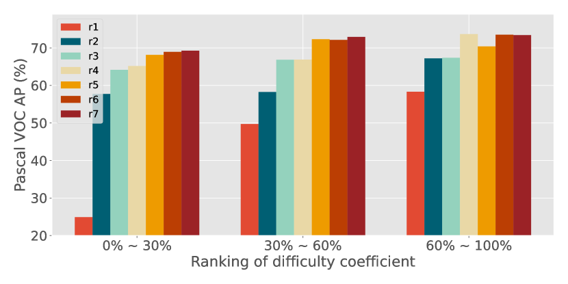
where $k$ is the training iteration, $d_{i}^{k}$ is the updated difficulty for category $i$, $N^{k}_{i}$ is the number of predicted objects of class $i$ in the training batch, $m_{i}^{*}$ is the EMA momentum, $m^{0}$ is the initial momentum for all categories. If a training batch does not contain objects in category $i$, we decrease its class-wise momentum by multiplying $m^{0}$ (Eq. 3), which ensures a similar updating pace of difficulties of different classes. In Fig. 2, we show how the class-wise difficulties correspond to the class-wise detection APs during the active learning process.

After training the detector on the labelled dataset, we compute the category-wise difficulty coefficient $W^{r}=\{w_{i}\}_{i\in[C]}$ for the $r$-th AL round as:

$$w_{i}=1+\alpha\beta\cdot\log{(1+\gamma\cdot d_{i})}$$ (4)

$$\text{where~{}~{}~{}~{}}\gamma=e^{1/\alpha}-1$$

where $\alpha$ controls how fast the difficulty coefficient changes w.r.t. the class-wise difficulty and $\beta$ controls the upper bound of the difficulty coefficient. Finally, we compute the image-wise uncertainty of every unlabelled image by summing the entropy of each detected object weighted by the corresponding difficulty coefficient:

$$U(I)=\sum_{i=1}^{M_{I}}w_{c(i)}\cdot\sum_{j=1}^{C^{\prime}}{-p_{ij}\cdot\log(p_{ij})}$$ (5)

where $M_{I}$ is the number of detected objects from image $I$; $w_{c(i)}$ is the weight of object $i$’s predicted category; $C^{\prime}$ is the number of classification ways, which is usually $C+1$ for two-stage detectors and $2$ for one-stage detectors; $p_{ij}$ is the predicted probability of category $j$. Finally, we use a simple strategy to select the candidate pool: for a given AL budget $b$, we select $\delta\cdot b$ images from the unlabelled set where we call the hyper-parameter $\delta>1$ the budget expanding ratio.

3.4 Diversity Sampling for Multi-instance Images

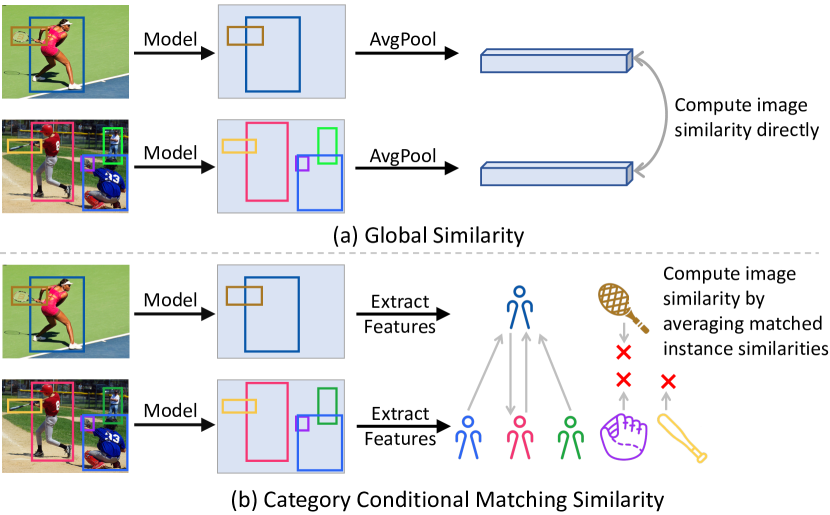
In the second stage of PPAL a diverse and representative set is be selected from the candidate pool to serve as the AL query set. In previous work [38, 1], diversity-based sampling is achieved by finding a subset of samples for which the similarities of each pair are minimised. Such similarities are often computed by the cosine or $L_{2}$ similarities of the averaged convolutional feature maps [38], which we call global similarity. This practice is simple and works well for object-centric datasets like ImageNet [36]. However, object detection usually take multi-instance images as input, and in such cases the averaged feature maps struggle to capture fine-grained spatial information in those images [43]. Because of this, we design a new method for computing similarities between multi-instance images, which can be used off-the-shelf for diversity-based sampling. We show the differences between the two approaches in Fig. 3.

Category Conditioned Matching Similarity. The intuition behind our CCMS is that the similarity of two multi-instance images can be computed by measuring how similar the objects they contain are. Formally, for two multi-instance images $I_{a}$ and $I_{b}$, the object detector detects several objects from them $O_{a}=\{o_{a,i}\}_{i\in[M_{a}]}$ and $O_{b}=\{o_{b,i}\}_{i\in[M_{b}]}$, in which each object $o_{*,i}$ is a triplet $o_{*,i}=(f_{*,i},t_{*,i},c_{*,i})$: $f_{*,i}$ is the object’s visual features extracted from the feature maps; $t_{*,i}$ is the detection score; $c_{*,i}$ is the predicted class label. We use the similarity of $O_{a}$ and $O_{b}$ as a proxy for the similarity of $I_{a}$ and $I_{b}$, which is computed by matching every object to its most similar counterpart in the same category in the other image. Specifically, for an object $o_{a,i}$ in $O_{a}$, its similarity to $O_{b}$ is computed as:

$$s(o_{a,i},O_{b})=\begin{cases}\underset{c_{b,j}=c_{a,i}}{\max}\frac{f_{a,i}\cdot f_{b,j}}{||f_{a,i}||\cdot||f_{b,j}||}+1\\ ~{}~{}~{}~{}~{}0~{}~{}~{}~{}~{}\text{if no $c_{b,j}=c_{a,i}$}\end{cases}$$ (6)

where we set $S(o_{a,i},O_{b})$ to $0$ if no object in $O_{b}$ is in the same category as $o_{a,i}$. Then the similarity of $O_{a}$ to $O_{b}$ is computed by averaging the object similarities weighted by their detection scores:

$$S^{\prime}(O_{a},O_{b})=\frac{1}{\sum_{i}{t_{a,i}}}\sum_{i=1}^{M_{a}}{t_{a,i}\cdot s(o_{a,i},O_{b})}$$ (7)

$$S(O_{a},O_{b})=\frac{1}{2}\cdot\bigl{(}S^{\prime}(O_{a},O_{b})+S^{\prime}(O_{b},O_{a})\bigr{)}$$

where the final similarity is the average of $S^{\prime}(O_{a},O_{b})$ and $S^{\prime}(O_{b},O_{a})$, which ensures the symmetry of the similarity.

Figure 4: A comparison between the proposed method and the state-of-the-art active learning algorithm for object detection in three different benchmark settings. (a) RetinaNet on COCO; (b) RetinaNet of Pascal VOC; (c) Faster R-CNN on COCO.

Figure 5: Comparison between the proposed method and the state-of-the-art active learning algorithm for object detection on Pascal VOC with SSD object detector.

Sampling AL Queries. We use the proposed CCMS to sample representative image set from the candidate pool as the AL query $Q$. The objective of the diversity-based sampling is formally written as:

$$Q=\underset{Q^{\prime}\subseteq H:|Q^{\prime}|=b}{\min}\Bigl{\{}\underset{I_{i},I_{j}\in Q^{\prime}}{\max}S(O_{i},O_{j})\Bigr{\}}$$ (8)

where $H$ is the candidate pool output from the first stage, and $b$ is the AL budget. However, Eq. 8 is an NP-Hard problem [38], so we follow [38] to use the k-Center-Greedy algorithm to get a 2-opt solution. Another problem with the objective in Eq. 8 is that it only maximises the diversity of the selected samples while ignoring how representative they are, which may cause the selection to favour data outliers. To deal with the problem, we further run a k-means++ algorithm using the results of k-Center-Greedy algorithm as the initial centroids. However, here we can only compute the similarities of every pair of images and are not able to compute the actual mean of every cluster to update its centroids. We solve this problem by assigning the new centroids as the images whose summed similarities to other images in their cluster are maximised. Finally, the resulting active learning queries are sent to human experts for annotation.

Figure 6: Active learning performance on Pascal VOC using three recently proposed object detectors. (a) Anchor-free FCOS; (b) Anchor-based ATSS; (c) Anchor-based DDOD.

Figure 7: Active learning performance on COCO using three recently proposed object detectors. (a) Anchor-free FCOS; (b) Anchor-based ATSS; (c) Anchor-based DDOD.

4 Experiments

4.1 Experiment Settings

Dataset settings. We benchmark Plug and Play Active Learning using two datasets: COCO [26] and Pascal VOC [14]. We follow the training and testing settings in MIAL [46]. Specifically, for COCO we use train2017 set for training, and evaluate the models on the mini-val set. 2% of the training images are randomly selected for initial training, and we run 4 rounds of active learning where at each round a further 2% of the training images are selected, annotated, and added into the training set. For Pascal VOC, we use train2007+2012 for training and test2007 for testing. We randomly sample 5% of the training data as the initial set, and we run 6 rounds of active learning where at each round 2.5% extra data are queried. We run all experiments using three different initial training sets and report the mean performance.

Model settings. We follow MIAL [46] to set our model and training recipes for fair comparison. We built our code-base using MMDetection toolkit [8]. For both dataset, the default training setting is to train the models for 26 epochs and decay the learning rate by 0.1 at the 20th epoch. We use ResNet-50 [18] as the default backbone network. All experiments are conducted using 8 NVIDIA 2080Ti GPUs. For both datasets we follow [9] and set $\xi$ in Eq.1 to 0.6, base EMA momentum $m^{0}$ to to 0.99, $\alpha$ and $\beta$ in Eq.4 to 0.3 and 0.2, and the budget expansion ratio $\delta$ to 4. We run the kmeans++ algorithm for 100 iterations. Note that all hyper-parameters are set empirically without careful tuning.

4.2 Main Results

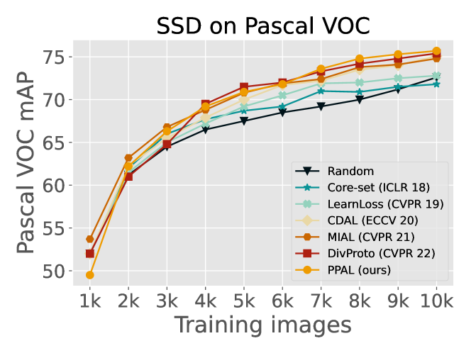
Comparing with the state-of-the-art. In Fig.4, we compare our PPAL with previous state-of-art active learning strategies on three different settings: COCO RetinaNet [33], Pascal VOC RetinaNet [25], and COCO Faster R-CNN [33]. We follow the default training recipe for the first two settings and for COCO Faster R-CNN we follow [42] to train the model with 12 epochs. For the entropy-based sampling strategy, we sum up the classification entropy of all detected objects as the image uncertainty, which results in a better performance than previous works [12, 46, 10] that compute image-wise uncertainty using the averaged or the maximum object entropy. As shown by the results, our PPAL outperforms all computing methods in all three settings. Specifically, in the initial rounds ($\leq$ 3), our method outperforms all competing methods by large margins, e.g., it outperforms MIAL [46] by 3.4 AP and 2.8 mAP on COCO and Pascal VOC respectively, which suggests that PPAL can provide the detectors with highly informative samples when they are not well trained. In the later rounds ($>$ 3), although the AP gaps between PPAL and the competing methods decrease, it still maintains the lead. In addition to PPAL’s ability to mine informative data samples, it also owns a better generalisation ability than the competing methods [46, 45], because it does not modify the model architecture or training pipeline. In Tab.5, we compare PPAL with previous works on Pascal VOC using the SSD [27] detector. We follow the training recipes in MIAL [46] to train the model for 300 epochs at each active learning round. Unlike other detectors [33, 25] that were used in the main paper, in SSD objects detected from different feature levels are computed using different convolutional kernels. In this case, we are unable to compute those objects’ distances using their visual features, so we follow CDAL [1] to compute the distances of their classification probability vectors using KL-divergence. The experiment results are reported in Figure 5. The results show that PPAL is able to achieve a better performance than all competing methods. Notably, although the initial performance of our SSD model is inferior to others, our active learning approach can still enable the model to surpass others in the later stages.

Performance on other detectors. Our PPAL is highly generalisable, which allows us to easily apply it to different object detectors. In Fig.6 and Fig. 7, we show the Pascal VOC and COCO results when applying it to three recently proposed object detectors: FCOS [40], ATSS [48] and DDOD [9], in which FCOS is anchor-free, and the rest are anchor-based. We also shows the results of three baselines: Random, Entropy (uncertainty-based), and Core-set [38] (diversity-based). The results show that PPAL is consistently better than the baselines for all three detectors, verifying its effectiveness and good generalisation ability.

4.3 Ablation Studies

In this section, we conduct ablation studies using Pascal VOC RetinaNet to study the proposed modules and the corresponding hyper-parameter settings.

Difficulty Calibrated Uncertainty Sampling. As shown in Tab.1, we start to study the proposed DCUS by first comparing it with the entropy-based sampling while disabling the second-stage diversity-based sampling. The results show that DCUS is consistently better than entropy-based sampling at all AL rounds. Then we compare DCUS with random sampling and entropy-based sampling by using those strategies to sample the candidate pool and run the diversity-based sampling using our CCMS for similarity computing. We find that DCUS still achieves a better performance, which validates DCUS’s effectiveness as an uncertainty-based AL strategy.

Category Conditioned Matching Similarity. As shown in Tab.1, we compare the proposed CCMS with three alternatives: (1) Rand, using random selection for the second stage; (2) Global, global similarity computed as the cosine similarity of the averaged feature maps from the backbone network’s last layer; (3) FPN, the averaged global similarity of every feature pyramid layer. Note that nearly all previous works [46, 38] use global similarity for diversity sampling. We observe that the global similarity works even worse than random selection, demonstrating its failure in measuring the similarity of multi-instance images. The FPN similarity works slightly better than the global similarity and generates similar performance with random sampling. Our CCMS achieves the best result, which is consistently better than the three alternatives. In addition, we find that diversity-based sampling is more important in later rounds of active learning: even CCMS achieves a similar performance with random sampling in the first two rounds, but their performance gap starts to increase from the third round. In conclusion, the benchmark results validate that the proposed CCMS is more suitable to measure the similarities of multi-instance images in active learning.

Size of the candidate pool. In Tab.2, we show how the budget expanding ratio $\delta$, which determines the size of the candidate pool, affects PPAL’s performance using Pascal VOC RetinaNet. We observe that when $\delta$ is around 4 our method can achieve the best performance. Specifically, we find that a too large $\delta$, like $\delta\geq 6$, will harm PPAL’s performance in early rounds, because in such cases the candidate pool will include many samples that the model is certain on, harming the overall information gain. On the other hand, a too-small expanding ratio, like $\delta<3$, will harm PPAL’s performance in later rounds because of the lacking of sample diversity in such small candidate pools.

Stage 1	Stage 2	mAP on % of labelled images
		5%	7.5%	10%	12.5%	15%	17.5%	20%
Random		43.4	51.5	57.6	60.7	63.9	66.3	66.6
Entropy	None	43.4	58.5	63.2	67.1	68.3	70.4	70.9
DCUS	None	43.4	60.5	64.4	67.2	68.7	70.4	71.6
Rand	CCMS	43.4	56.6	61.2	64.7	66.9	68.4	70.3
Entropy	CCMS	43.4	59.0	64.5	67.6	69.2	71.1	72.0
DCUS	Rand	43.4	60.3	64.1	67.6	68.9	70.5	72.0
DCUS	Global	43.4	58.8	64.5	66.9	68.6	69.3	71.8
DCUS	FPN	43.4	59.4	64.3	67.3	68.6	70.0	71.6
DCUS	CCMS	43.4	60.8	66.2	68.4	70.5	71.6	72.6

Table 1: An ablation study for the proposed Difficulty Calibrated Uncertainty Sampling (DCUS) and Category Conditioned Matching Similarity (CCMS) using Pascal VOC RetinaNet.

Pool Size	mAP on % of labelled images
($\delta$)	5%	7.5%	10%	12.5%	15%	17.5%	20%
1	43.4	60.5	64.4	67.2	68.7	70.4	71.6
2	43.4	60.4	65.8	67.6	69.0	70.6	71.5
3	43.4	60.5	65.4	67.7	70.0	71.3	71.8
4	43.4	60.8	66.2	68.4	70.5	71.6	72.6
5	43.4	61.2	65.0	68.0	70.1	71.4	72.6
6	43.4	59.8	65.9	67.9	70.1	71.4	72.3

Table 2: An ablation study on how the budget expanding ratio $\delta$, which determines the size of the candidate pool in the first-stage, affect PPAL’s performance using Pascal VOC RetinaNet.

Figure 8: A hyper-parameter ablation study on $\alpha$ and $\beta$ in our DCUS using Pascal VOC RetinaNet. We fixed $\alpha=0.3$ and $\beta=0.2$ when studying the other parameter.

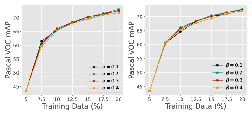
Hyper-parameters in computing difficulty coefficient. In Fig.2, we show how the two hyper-parameters in Eq.1 affect PPAL’s performance. They are $\alpha$, which controls how fast the difficulty coefficient changes with the class-wise difficulty, and $\beta$, which controls the upper-bound of difficulty coefficients. We observe that PPAL’s performance is robust quite robust when $\alpha\leq 0.3$, but a large $\alpha$ will harm the model accuracy at all rounds. On the other hand, we found a small $\beta$ will cause inferior performance in early rounds. In such cases, the small $\beta$ generates similar difficulty coefficients for all classes, so classes with different difficulties will make similar contributions in the uncertainty-based sampling and harm the AL effectiveness. Also, a too large $\beta$ can also result in inferior performance because the easy categories would be largely ignored.

Uncertainty	mAP on % of labelled images
	5%	7.5%	10%	12.5%	15%	17.5%	20%
Random	43.4	51.5	57.6	60.7	63.9	66.3	66.6
Posterior	43.4	60.8	66.0	68.7	71.2	71.5	72.3
Margin	43.4	59.9	66.1	67.8	70.8	71.4	72.8
Entropy	43.4	60.8	66.2	68.4	70.5	71.6	72.6

Table 3: A comparison of different uncertainty measurements on Pascal VOC RetinaNet using the proposed PPAL.

Backbone	Method	mAP on % of labelled images
		5%	7.5%	10%	12.5%	15%	17.5%	20%
ResNet101	Rand	51.0	59.3	64.6	68.4	69.8	71.0	72.3
	PPAL	51.0	64.3	69.6	71.1	72.8	73.8	75.0
MobileNetV2	Rand	20.9	31.2	31.4	39.7	42.8	42.9	44.7
	PPAL	20.9	35.7	41.9	45.6	46.3	48.4	50.7
SwinTiny	Rand	59.0	63.8	67.9	70.0	71.2	71.8	73.3
	PPAL	59.0	68.4	71.2	72.7	74.8	75.4	76.2

Table 4: Performance of the proposed PPAL on Pascal VOC RetinaNet using different backbone networks.

Figure 9: A comparison between global similarity and the proposed CCMS on image retrieval using RetinaNet on COCO mini-val. We retrieve 20 most similar images for each anchor image. The similarity numbers are normalised to $(0,1)$.

Figure 10: Image retrieval visualisation using global similarity and the proposed CCMS on COCO mini-val using RetinaNet.

4.4 Discussions

Uncertainty Measurement. As presented in Sec.3.3, in PPAL we use entropy as the default uncertainty measurement. In Tab.3, we show that our method can achieve similar performance when generalising to other types of uncertainty measurement. Specifically, we test PPAL on Pascal VOC RetinaNet using two alternative uncertainty measurements: posterior probability [22] and probability margin [11]. We observe that the posterior probability has a very close performance to entropy. However, the probability margin achieves an inferior performance in the early rounds, but can get similar performances with the other two uncertainty measurements in later rounds.

Generalising to different backbones. In Tab.4, we show our approach can well generalise to other backbone networks. We test PPAL on Pascal VOC RetinaNet using the heavy-weighted ResNet-101 [18], light-weighted MobileNet v2 [37] and the high-performing transformer based SwinTransformer-Tiny [28]. The results show that PPAL is consistently better than random sampling by a large margin in all those backbone architectures, validating the strong generalisation ability of our approach.

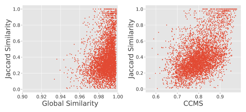
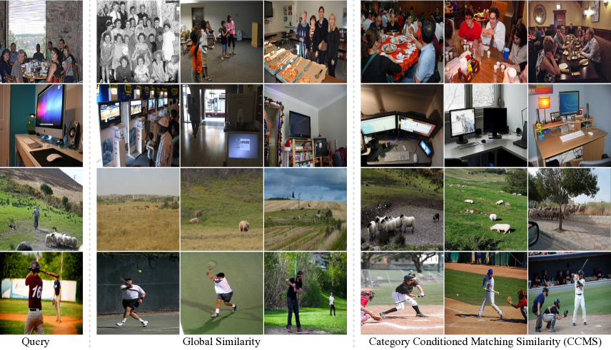
Why is CCMS better than global similarity? Here we investigate why the proposed CCMS is better than global similarity in measuring image-wise similarity for multi-instance images by running an image retrieval experiment on COCO mini-val set using a pre-trained RetinaNet detector: For each anchor image, we use both means of computing similarity to retrieve the 20 most similar images. Then we check whether the retrieved images depict similar scenes with the anchor image by measuring the averaged Jaccard similarity of object categories contained in those images. Specifically, for image $I_{i}$ and $I_{j}$ and their contained object category set $C_{i}$ and $C_{j}$, their Jaccard similarity is defined as $\mathcal{J}_{ij}=\frac{|C_{i}\cap C_{j}|}{|C_{i}\cup C_{j}|}$. For example, if an image contains $\{$dog, human$\}$ and the other image contains $\{$dog, cat$\}$, their Jaccard similarity $0.33$. We show the result on the whole COCO mini-val set in Fig.9. We observe that the averaged CCMS and Jaccard similarity are positively correlated, i.e., a high averaged CCMS usually corresponds to a high averaged Jaccard similarity and vice versa. However, global similarity does not hold such correspondence to the class-wise Jaccard similarity. In Fig.10, we show the image retrieval results by visualising the 3 most similar images with the anchor. From it we get two observations: (1) Global similarity is usually biased toward the dominating objects in the image while ignoring other objects (1st and 2nd rows) and CCMS is not; (2) CCMS is better than global similarity in capturing the fine-grained details in the image (3rd and 4th rows). These results validate our argument that CCMS is a more suitable similarity computing method for diversity-based active learning for object detection, which usually uses multi-instance images as input.

5 Conclusion

This work introduces Plug and Play Active Learning (PPAL), an effective two-stage active learning algorithm for object detection. In the first stage, we propose Difficulty Calibrated Uncertainty Sampling to select a candidate pool of uncertain samples, and in the second stage we select a diverse and representative active learning query set using the proposed Category Conditioned Matching Similarity. The experiments show PPAL can generalise well and outperform previous works in various architectures and datasets.

Acknowledgements.

Chenhongyi Yang was supported by a PhD studentship provided by the School of Engineering, University of Edinburgh.

References

- [1] Sharat Agarwal, Himanshu Arora, Saket Anand, and Chetan Arora. Contextual diversity for active learning. In ECCV, 2020.
- [2] Jordan T Ash, Chicheng Zhang, Akshay Krishnamurthy, John Langford, and Alekh Agarwal. Deep batch active learning by diverse, uncertain gradient lower bounds. In ICLR, 2020.
- [3] Mustafa Bilgic and Lise Getoor. Link-based active learning. In NeurIPS Workshop on Analyzing Networks and Learning with Graphs, 2009.
- [4] Qi Cai, Yingwei Pan, Yu Wang, Jingen Liu, Ting Yao, and Tao Mei. Learning a Unified Sample Weighting Network for Object Detection. In CVPR, 2020.
- [5] Zhaowei Cai and Nuno Vasconcelos. Cascade r-cnn: Delving into high quality object detection. In CVPR, 2018.
- [6] Nicolas Carion, Francisco Massa, Gabriel Synnaeve, Nicolas Usunier, Alexander Kirillov, and Sergey Zagoruyko. End-to-End Object Detection with Transformers. ECCV, 2020.
- [7] Kai Chen, Jiangmiao Pang, Jiaqi Wang, Yu Xiong, Xiaoxiao Li, Shuyang Sun, Wansen Feng, Ziwei Liu, Jianping Shi, Wanli Ouyang, et al. Hybrid task cascade for instance segmentation. In CVPR, 2019.
- [8] Kai Chen, Jiaqi Wang, Jiangmiao Pang, Yuhang Cao, Yu Xiong, Xiaoxiao Li, Shuyang Sun, Wansen Feng, Ziwei Liu, Jiarui Xu, Zheng Zhang, Dazhi Cheng, Chenchen Zhu, Tianheng Cheng, Qijie Zhao, Buyu Li, Xin Lu, Rui Zhu, Yue Wu, Jifeng Dai, Jingdong Wang, Jianping Shi, Wanli Ouyang, Chen Change Loy, and Dahua Lin. MMDetection: Open mmlab detection toolbox and benchmark. arXiv preprint arXiv:1906.07155, 2019.
- [9] Zehui Chen, Chenhongyi Yang, Qiaofei Li, Feng Zhao, Zheng-Jun Zha, and Feng Wu. Disentangle your dense object detector. In ACM MM, 2021.
- [10] Jiwoong Choi, Ismail Elezi, Hyuk-Jae Lee, Clement Farabet, and Jose M Alvarez. Active learning for deep object detection via probabilistic modeling. In ICCV, 2021.
- [11] Gui Citovsky, Giulia DeSalvo, Claudio Gentile, Lazaros Karydas, Anand Rajagopalan, Afshin Rostamizadeh, and Sanjiv Kumar. Batch active learning at scale. ICLR, 2021.
- [12] Ismail Elezi, Zhiding Yu, Anima Anandkumar, Laura Leal-Taixe, and Jose M Alvarez. Not all labels are equal: Rationalizing the labeling costs for training object detection. In CVPR, 2022.
- [13] Ehsan Elhamifar, Guillermo Sapiro, Allen Yang, and S Shankar Sasrty. A convex optimization framework for active learning. In ICCV, 2013.
- [14] Mark Everingham, SM Ali Eslami, Luc Van Gool, Christopher KI Williams, John Winn, and Andrew Zisserman. The Pascal Visual Object Classes Challenge: A Retrospective. IJCV, 2015.
- [15] Yarin Gal, Riashat Islam, and Zoubin Ghahramani. Deep bayesian active learning with image data. In ICML. PMLR, 2017.
- [16] Yuhong Guo. Active instance sampling via matrix partition. NeurIPS, 2010.
- [17] Kaiming He, Georgia Gkioxari, Piotr Dollár, and Ross Girshick. Mask r-cnn. In ICCV, 2017.
- [18] Kaiming He, Xiangyu Zhang, Shaoqing Ren, and Jian Sun. Deep residual learning for image recognition. In CVPR, 2016.
- [19] Lichao Huang, Yi Yang, Yafeng Deng, and Yinan Yu. DenseBox: Unifying landmark localization with end to end object detection. arXiv preprint arXiv:1509.04874, 2015.
- [20] Ajay J Joshi, Fatih Porikli, and Nikolaos Papanikolopoulos. Multi-class active learning for image classification. In CVPR, 2009.
- [21] Alina Kuznetsova, Hassan Rom, Neil Alldrin, Jasper Uijlings, Ivan Krasin, Jordi Pont-Tuset, Shahab Kamali, Stefan Popov, Matteo Malloci, Alexander Kolesnikov, et al. The open images dataset v4. IJCV, 128(7):1956–1981, 2020.
- [22] David D Lewis and Jason Catlett. Heterogeneous uncertainty sampling for supervised learning. In Machine learning proceedings, pages 148–156. Elsevier, 1994.
- [23] David D Lewis and William A Gale. A sequential algorithm for training text classifiers. In SIGIR, pages 3–12. Springer, 1994.
- [24] Feng Li, Hao Zhang, Shilong Liu, Jian Guo, Lionel M Ni, and Lei Zhang. Dn-detr: Accelerate detr training by introducing query denoising. In CVPR, 2022.
- [25] Tsung-Yi Lin, Priya Goyal, Ross Girshick, Kaiming He, and Piotr Dollár. Focal loss for dense object detection. In ICCV, 2017.
- [26] Tsung-Yi Lin, Michael Maire, Serge Belongie, James Hays, Pietro Perona, Deva Ramanan, Piotr Dollár, and C Lawrence Zitnick. Microsoft coco: Common objects in context. In ECCV, 2014.
- [27] Wei Liu, Dragomir Anguelov, Dumitru Erhan, Christian Szegedy, Scott Reed, Cheng-Yang Fu, and Alexander C Berg. Ssd: Single shot multibox detector. In ECCV, 2016.
- [28] Ze Liu, Yutong Lin, Yue Cao, Han Hu, Yixuan Wei, Zheng Zhang, Stephen Lin, and Baining Guo. Swin transformer: Hierarchical vision transformer using shifted windows. In Proceedings of the IEEE/CVF International Conference on Computer Vision, pages 10012–10022, 2021.
- [29] Wenjie Luo, Alex Schwing, and Raquel Urtasun. Latent structured active learning. NeurIPS, 2013.
- [30] Oisin Mac Aodha, Neill DF Campbell, Jan Kautz, and Gabriel J Brostow. Hierarchical subquery evaluation for active learning on a graph. In CVPR, 2014.
- [31] Viraj Prabhu, Arjun Chandrasekaran, Kate Saenko, and Judy Hoffman. Active domain adaptation via clustering uncertainty-weighted embeddings. In ICCV, 2021.
- [32] Joseph Redmon and Ali Farhadi. Yolov3: An incremental improvement. arXiv preprint arXiv:1804.02767, 2018.
- [33] Shaoqing Ren, Kaiming He, Ross Girshick, and Jian Sun. Faster r-cnn: Towards real-time object detection with region proposal networks. In NeurIPS, 2015.
- [34] Hamid Rezatofighi, Nathan Tsoi, JunYoung Gwak, Amir Sadeghian, Ian Reid, and Silvio Savarese. Generalized Intersection Over Union: A Metric and a Loss for Bounding Box Regression. In CVPR, 2019.
- [35] Dan Roth and Kevin Small. Margin-based active learning for structured output spaces. In ECML. Springer, 2006.
- [36] Olga Russakovsky, Jia Deng, Hao Su, Jonathan Krause, Sanjeev Satheesh, Sean Ma, Zhiheng Huang, Andrej Karpathy, Aditya Khosla, Michael Bernstein, Alexander C. Berg, and Li Fei-Fei. ImageNet Large Scale Visual Recognition Challenge. IJCV, 2015.
- [37] Mark Sandler, Andrew Howard, Menglong Zhu, Andrey Zhmoginov, and Liang-Chieh Chen. Mobilenetv2: Inverted Residuals and Linear Bottlenecks. In CVPR, 2018.
- [38] Ozan Sener and Silvio Savarese. Active learning for convolutional neural networks: A core-set approach. ICLR, 2018.
- [39] Burr Settles. Active learning. Synthesis lectures on artificial intelligence and machine learning, 6(1):1–114, 2012.
- [40] Zhi Tian, Chunhua Shen, Hao Chen, and Tong He. Fcos: Fully convolutional one-stage object detection. In ICCV, 2019.
- [41] Keze Wang, Dongyu Zhang, Ya Li, Ruimao Zhang, and Liang Lin. Cost-effective active learning for deep image classification. T-CSVT, 27(12):2591–2600, 2016.
- [42] Jiaxi Wu, Jiaxin Chen, and Di Huang. Entropy-based active learning for object detection with progressive diversity constraint. In CVPR, 2022.
- [43] Chenhongyi Yang, Lichao Huang, and Elliot J Crowley. Contrastive object-level pre-training with spatial noise curriculum learning. arXiv preprint arXiv:2111.13651, 2021.
- [44] Yi Yang, Zhigang Ma, Feiping Nie, Xiaojun Chang, and Alexander G Hauptmann. Multi-class active learning by uncertainty sampling with diversity maximization. IJCV, 113(2):113–127, 2015.
- [45] Donggeun Yoo and In So Kweon. Learning loss for active learning. In CVPR, 2019.
- [46] Tianning Yuan, Fang Wan, Mengying Fu, Jianzhuang Liu, Songcen Xu, Xiangyang Ji, and Qixiang Ye. Multiple instance active learning for object detection. In CVPR, 2021.
- [47] Hao Zhang, Feng Li, Shilong Liu, Lei Zhang, Hang Su, Jun Zhu, Lionel M Ni, and Heung-Yeung Shum. Dino: Detr with improved denoising anchor boxes for end-to-end object detection. arXiv preprint arXiv:2203.03605, 2022.
- [48] Shifeng Zhang, Cheng Chi, Yongqiang Yao, Zhen Lei, and Stan Z Li. Bridging the gap between anchor-based and anchor-free detection via adaptive training sample selection. In CVPR, 2020.
- [49] Fedor Zhdanov. Diverse mini-batch active learning. arXiv preprint arXiv:1901.05954, 2019.
- [50] Xizhou Zhu, Weijie Su, Lewei Lu, Bin Li, Xiaogang Wang, and Jifeng Dai. Deformable detr: Deformable transformers for end-to-end object detection. In ICLR, 2020.