Radion dynamics in multibrane Randall-Sundrum model

Abstract

The radion in the Randall-Sundrum model is stabilized by the back reaction of a bulk scalar field with its VEV depending on the fifth dimensional coordinate. We studied the radion dynamics in an extended scenario, where intermediate branes exist between the UV and IR branes. Our analysis proves that the formalism of EFT delivers the same equations of motion as the linearized Einstein equation with all junction conditions satisfied. The relic of 5d diffeomorphism is broken after including the Goldberger-Wise stabilization and a unique radion field is conjectured as legitimate in the RS metric perturbation.

1 5d warped model

The Randall-Sundrum (RS) model compacted in a slice of anti–de-Sitter (AdS) space with 2 branes can naturally illustrate the emerging of TeV energy scale and the weakness of gravity [1]. The multibrane RS model is an appealing extension since a new energy scale between the Planck and TeV ones is plausible for phenomenology study [2]. The $N$-brane ($N\in$ even integer) extension of RS model can be achieved given that the cosmology constants $\Lambda_{\alpha}$, $\alpha=1,\cdots\frac{N}{2}$ are different in each subregion of an AdS₅ space. We start with the generic five dimensional action with an orbifold symmetry for the graviton coupling to a single bulk scalar field [3, 4]:

$$S=S_{EH}+S_{m}=-\frac{1}{2\kappa^{2}}\int d^{5}x\sqrt{g}\,{\cal R}+\int d^{5}x\sqrt{g}\mathcal{L}_{m}\,,$$ (1)

$$\mathcal{L}_{m}=\frac{1}{2}g^{IJ}\partial_{I}\phi\partial_{J}\phi-V(\phi)-\frac{1}{\sqrt{-g_{55}}}\sum_{i=1}^{N}\lambda_{i}(\phi)\delta(y-y_{i})$$ (2)

where the first term in Eq.(1) is the Einstein-Hilbert action, and the second one is the matter action. For simplicity we refer all objects located at $y_{i}$,$i=1,\cdots N$ as branes like in the original RS model. With appropriate bulk and brane potentials $V(\phi)$ and $\lambda_{i}$, the scalar $\phi=\phi_{0}(y)+\varphi(x,y)$ develops a $y$-dependent VEV that reacts back on the metric. As a result, the radion field will obtain a mass via the Goldberger-Wise (GW) mechanism [5]. The line element in an $N$-brane model decoupling the graviton and radion is [2, 6]:

$$ds^{2} = e^{-2A(y)-2F(x,y)}\left[\eta_{\mu\nu}+2\epsilon(y)\partial_{\mu}\partial_{\nu}f(x)\right.$$ (3)

$$+ \left.h_{\mu\nu}(x,y)\right]dx^{\mu}dx^{\nu}-\left[1+G(x,y)\right]^{2}dy^{2}\,,$$

where the $\epsilon(y)$ is added as a radion perturbation in addition to $F$ and $G$. By varying the 5d action with respect to the metric $g_{IJ}$, one can derive the Einstein equation: $\mathcal{R}_{IJ}=\kappa^{2}\left(T_{IJ}-\frac{1}{3}g_{IJ}T^{m}_{m}\right)=\kappa^{2}\tilde{T}_{IJ}$, with the energy-momentum tensor defined as $T_{IJ}=2\delta(\sqrt{g}\mathcal{L}_{m})/(\sqrt{g}\delta g^{IJ})$. While minimizing $S_{m}$ with respect to $\varphi$ gives the scalar EOM, that at the linear order is modified by a term $\phi^{\prime}_{0}\epsilon^{\prime}\Box f(x)$ in our metric [7]. But the solutions for background metric and scalar VEV $\phi_{0}$ are the same as in RS1 and can be written in terms of a single super-potential $W(\phi)$ as [3, 8]:

$$\phi_{0}^{\prime}=\frac{1}{2}\frac{\partial W}{\partial\phi}\,,\quad A^{\prime}=\frac{\kappa^{2}}{6}W(\phi_{0})\,,\quad V(\phi)=\frac{1}{8}\left[\frac{\partial W(\phi)}{\partial\phi}\right]^{2}-\frac{\kappa^{2}}{6}W(\phi)^{2}$$ (4)

We are going to investigate the graviton-scalar system in the formalism of effective Lagrangian and practice the variation principle to a specific perturbation field. In fact the scalar EOM has to be derived in this approach as it is not contained in the Einstein equation. Expanding the 5d action Eq.(1) till the quadratic order, we obtain the effective Lagrangian [7]:

$$\mathcal{L}_{eff} = \int dy\Big{\{}\frac{e^{-2A}}{2\kappa^{2}}\Big{[}\frac{e^{-2A}}{4}\left[(\partial_{5}h)^{2}-\partial_{5}h_{\mu\nu}\,\partial_{5}h^{\mu\nu}\right]-{\mathcal{L}}_{FP}\Big{]}$$ (5)

$$+ {\mathcal{L}}_{mix}\,+\,\mathcal{L}_{r-kin}-\frac{e^{-4A}}{2}\mathcal{L}_{5m}\Big{\}}\,$$

where the terms in the first line are for the graviton with:

$${\mathcal{L}}_{FP}=\frac{1}{2}\partial_{\nu}h_{\mu\alpha}\,\partial^{\alpha}h^{\mu\nu}-\frac{1}{4}\partial_{\mu}h_{\alpha\beta}\,\partial^{\mu}h^{\alpha\beta}-\frac{1}{2}\partial_{\alpha}h\,\partial_{\beta}h^{\alpha\beta}+\frac{1}{4}\partial_{\alpha}h\,\partial^{\alpha}h\,$$ (6)

The second line in Eq.(5) contains the graviton-radion mixing term along with the kinetic and non-kinetic terms of radion:

$$\mathcal{L}_{mix} = -\frac{e^{-2A}}{2\kappa^{2}}\left[\left[G-2F-e^{2A}\partial_{5}\left(\epsilon^{\prime}f(x)e^{-4A}\right)\right]\left(\partial_{\mu}\partial_{\nu}h^{\mu\nu}-\Box\,h\right)\right.$$ (7)

$$+ \left.3e^{-2A}\left[F^{\prime}-A^{\prime}G-\frac{\kappa^{2}}{3}\phi^{\prime}_{0}\varphi\right]\partial_{5}h\right]\,$$

$$\mathcal{L}_{r-kin} = \frac{1}{2}\int dye^{-2A}\kappa^{2}\partial_{\mu}\varphi\partial^{\mu}\varphi-\frac{6}{\kappa^{2}}\Big{[}\partial_{\mu}F\partial^{\mu}\left(F-G\right)$$ (8)

$$- e^{-2A}\epsilon^{\prime}\partial_{\mu}\left[F^{\prime}-A^{\prime}G-\frac{\kappa^{2}}{3}\phi^{\prime}_{0}\varphi\right]\partial^{\mu}f(x)\Big{]}$$

$$\mathcal{L}_{5m} = -\frac{12}{\kappa^{2}}\Big{[}F^{\prime 2}+G^{2}A^{\prime 2}-2F^{\prime}GA^{\prime}\Big{]}+\varphi^{\prime 2}+G^{2}\phi^{\prime 2}_{0}-2(G+4F)\phi^{\prime}_{0}\varphi^{\prime}$$ (9)

$$+ \left[2(G-4F)\frac{\partial V}{\partial\phi_{0}}\varphi+\frac{\partial^{2}V}{\partial\phi_{0}^{2}}\varphi^{2}\right]-\sum_{i=1}^{N}\Big{[}8\frac{\partial\lambda_{i}}{\partial\phi_{0}}F\varphi-\frac{\partial^{2}\lambda_{i}}{\partial\phi_{0}^{2}}\varphi^{2}\Big{]}\delta(y-y_{i})$$

Requiring no-mixing between the graviton and radion, one can immediately derive two orthogonal conditions from Eq.(7):

$$F^{\prime}-A^{\prime}G-\frac{\kappa^{2}}{3}\phi^{\prime}_{0}\varphi=0\,,$$ (10)

$$G-2F-e^{-2A}\left[\epsilon^{\prime\prime}-4A^{\prime}\epsilon^{\prime}\right]f(x)=0\,.$$ (11)

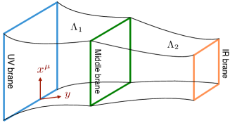
Figure 1: The $4$-brane RS model visualized in the range of $0\leq y\leq L$. An identical part exits in $-L\leq y<0$ due to the orbifold symmetry.

By varying Eq.(5) with respect to $F,G$ and $\varphi$, one can obtain 3 EOMs. We find that one exact correspondence can be established between 2 EOMs and the linearized Einstein equations, i.e.

$$\frac{\delta\mathcal{L}_{eff}}{\delta G}=0 \Rightarrow \frac{1}{\kappa^{2}}\left[e^{2A}\mathcal{R}_{\mu\nu}/\eta_{\mu\nu}+\mathcal{R}_{55}\right]=\left[e^{2A}\tilde{T}_{\mu\nu}/\eta_{\mu\nu}+\tilde{T}_{55}\right]\,,$$ (12)

$$\frac{\delta\mathcal{L}_{eff}}{\delta F}=0 \Rightarrow \frac{1}{2\kappa^{2}}\left[2e^{2A}\mathcal{R}_{\mu\nu}/\eta_{\mu\nu}-\mathcal{R}_{55}\right]=\left[e^{2A}\tilde{T}_{\mu\nu}/\eta_{\mu\nu}-\frac{1}{2}\tilde{T}_{55}\right]\,.$$ (13)

The 3rd one $\frac{\delta\mathcal{L}_{eff}}{\delta\varphi}=0$ gives the scalar EOM:

$$(G^{\prime}+4F^{\prime})\phi^{\prime}_{0}+4A^{\prime}\varphi^{\prime}+\sum_{i=1}^{N}\left(\frac{\partial\lambda_{i}}{\partial\phi_{0}}G+\frac{\partial^{2}\lambda_{i}}{\partial\phi_{0}^{2}}\varphi\right)\delta(y-y_{i})$$ (14)

$$= \varphi^{\prime\prime}-\left(2\frac{\partial V}{\partial\phi_{0}}G+\frac{\partial^{2}V}{\partial\phi_{0}^{2}}\varphi\right)-\Box\Big{(}\varphi e^{2A}-\phi^{\prime}_{0}\epsilon^{\prime}f(x)\Big{)}\,.$$

One can prove that Eq.(12-14) are correlated and a single EOM is independent [7]. With some algebra, Eq.(12) can be recasted into the familiar form [6]:

$$3\left(F^{\prime\prime}-A^{\prime}G^{\prime}\right)+3\left[Fe^{2A}-A^{\prime}\epsilon^{\prime}(y)\right]\Box f(x)$$ (15)

$$= 2\kappa^{2}\phi_{0}^{\prime}\varphi^{\prime}+\frac{\kappa^{2}}{3}\sum_{i=1}^{N}\left[3\lambda_{i}(\phi_{0})G+3\frac{\partial\lambda_{i}}{\partial\phi}\varphi\right]\delta(y-y_{i})$$

In fact only one EOM plus two orthogonal conditions are independent for 4 radion fields $F,G$, $\varphi$ and $\epsilon$, and this implies that one perturbation is a gauge fixing.

2 Breaking of 5d diffeomorphism

We will first review the 5d diffeomorphism that is an infinitesimal coordinate transformation $X^{I}\to X^{I}+\xi^{I}(X)$ which can keep $S_{EH}$ (not the full 5d action) to be invariant. As a result, the metric transforms accordingly:

$$\delta g_{IJ}=-\xi^{K}\,\partial_{K}g_{IJ}^{(0)}-\partial_{I}\xi^{K}\,g_{KJ}^{(0)}-\partial_{J}\xi^{K}\,g_{IK}^{(0)}\,.$$ (16)

To retain the metric in its original structure after a field redefinition, $\xi^{I}(X)$ is constrained to be of the specific form [2]:

$$\xi^{\mu}(x,y) = \hat{\xi}^{\mu}(x)+\,\eta^{\mu\nu}\partial_{\nu}\zeta(x,y)$$

$$\xi^{5}(x,y) = e^{-2A}\,\zeta^{\prime}(x,y)\,.$$ (17)

with $\zeta^{\prime}(x,y)|_{y=y_{i}}=0$. Hence the metric perturbations transform as:

$$\delta h_{\mu\nu}=-\partial_{\mu}\hat{\xi}_{\nu}-\partial_{\nu}\hat{\xi}_{\mu}$$

$$\delta F=-A^{\prime}\zeta^{\prime}e^{-2A}$$

$$\delta G=-\left(\zeta^{\prime\prime}-2A^{\prime}\zeta^{\prime}\right)e^{-2A}$$

$$\delta\epsilon f(x)=-\zeta\,$$ (18)

where the last ansatz indicates that $\epsilon f(x)$ plays the role of gauge fixing and can be removed by setting $\zeta=\epsilon f(x)$. However the situation becomes different after the radion stabilization. Inspecting Eq.(12-14), we can find that a field redefinition below can remove the $\epsilon$ dependence in all 3 EOMs:

$$\tilde{F} = F-A^{\prime}\epsilon^{\prime}f(x)e^{-2A}$$

$$\tilde{G} = G-\left(\epsilon^{\prime\prime}-2A^{\prime}\epsilon^{\prime}\right)f(x)e^{-2A}$$

$$\tilde{\varphi} = \varphi-\phi^{\prime}_{0}\epsilon^{\prime}f(x)e^{-2A}\,$$ (19)

where the first two are the same as in the diffeomorphism (see Eq.(18)) and the last one is for the GW scalar. As an invariant scalar, $\delta\varphi=0$ forces $\phi^{\prime}_{0}\,\epsilon^{\prime}=0$ otherwise the 4d Poincaré symmetry will be broken and ambiguity will enter in the radion kinetic term. Since we pursue a solution with a stabilized radion, the correct option is to let $\phi^{\prime}_{0}\neq 0$ and $\epsilon^{\prime}=0$ [7]. This signals that the 5d $\zeta$-symmetry is actually broken.

3 Stabilization and cosmology implication

The solvable radion EOM in a multibrane RS model is Eq.(15) gauged with $\epsilon^{\prime}=0$ and $G=2F$. We consider the simplest case $N=4$, and generalize the GW mechanism to the $4$-brane model by choosing the following superpotential,

$$W(\phi)=\begin{cases}\frac{6k_{1}}{\kappa^{2}}-u\phi^{2}\,,&0<y<r\\[8.5359pt] \frac{6k_{2}}{\kappa^{2}}-u\phi^{2}\,,&r<y<L\end{cases}\,$$ (20)

To solve the eigenstate problem, the stiff potentials will be imposed at the UV and IR branes similar to RS1 such that $\varphi|_{y=\{0,L\}}=0$. While at the intermediate brane $y=r$, we use the junction condition $\left[F^{\prime}\right]_{r}=2\left[A^{\prime}\right]_{r}F(r)$. Then for $l=\frac{\kappa\phi_{0}}{\sqrt{2}}|_{y=0}\ll 1$, the radion mass turns out to be $m^{2}\simeq\frac{4u^{2}(2k_{2}+u)l^{2}}{3k_{2}}e^{-2\left[(k_{2}+u)L+(k_{1}-k_{2})r\right]}$, that is below the cut off scale of IR brane. We can briefly discuss the cosmological evolution in the multibrane RS model by taking the metric to be time dependent [9, 10]:

$$ds^{2}\,=\,n(t,y)^{2}dt^{2}-a(t,y)^{2}dx^{2}-b(t,y)^{2}dy^{2}$$

$$a(t,y)=a_{0}(t)e^{-A}(1+\delta a)\,,~{}~{}n(t,y)=e^{-A}(1+\delta n)$$

$$b(t,y)=1+\delta b$$ (21)

with the perturbations $(\delta a,\delta n,\delta b)$ caused by adding the matter densities. Averaging the Einstein Equation $G_{55}=\kappa^{2}T_{55}$ with respect to $y=r$, one can derive [6]:

$$\left(\frac{\dot{a}_{0}}{a_{0}}\right)^{2}+\frac{\ddot{a}_{0}}{a_{0}}=\frac{\kappa^{2}e^{-2A}}{3}\left[\frac{k_{1}k_{2}}{k_{1}-k_{2}}\left(\rho-3p\right)+\phi^{\prime 2}_{0}\delta b\right]\,,$$ (22)

where $\rho$ and $p$ are the matter density and pressure at the $y=r$ brane. Because the intermediate brane essentially is a spacetime defect, one expects that $\delta b(r)$ is fixed by the initial condition. And Eq.(22) is a constraint that a multibrane system needs to observe.

4 Conclusion

We examine the radion dynamics in the multibrane RS model by adding a new radion perturbation $\epsilon\,\partial_{\mu}\partial_{\nu}f(x)$ in the metric. Our analysis shows that the formalism of effective Lagrangian is equivalent to the linearized Einstein equation and only a single radion EOM is actually independent no matter with or without stabilization. The role of $\epsilon$ is a gauge fixing for the Einstein-Hilbert action and can be removed by setting $\zeta=\epsilon f(x)$ using the 5d diffeomorphism. However this 5d symmetry has to be broken in order to preserve the 4d poincaré symmetry in the presence of radion stabilization. Thus $\epsilon^{\prime}=0$ holds in the full bulk with its boundary value $\epsilon^{\prime}(r)=0$, not possible to create a new radion excitation. The consequence of one radion permitted in the 5d action Eq.(1) renders the intermediate branes to be nondynamical. The unique radion profile is $F\propto e^{2A}+\mathcal{O}(l^{2})$, satisfying the jump condition $\left[F^{\prime}\right]_{r_{a}}=2\left[A^{\prime}\right]_{r_{a}}F(r_{a})$. Therefore we can simply generalize the GW mechanism into an $N$-brane extension in a way similar to RS1.