Neural networks trained with SGD learn distributions of increasing complexity

Abstract

The uncanny ability of over-parameterised neural networks to generalise well has been explained using various “simplicity biases”. These theories postulate that neural networks avoid overfitting by first fitting simple, linear classifiers before learning more complex, non-linear functions. Meanwhile, data structure is also recognised as a key ingredient for good generalisation, yet its role in simplicity biases is not yet understood. Here, we show that neural networks trained using stochastic gradient descent initially classify their inputs using lower-order input statistics, like mean and covariance, and exploit higher-order statistics only later during training. We first demonstrate this distributional simplicity bias (DSB) in a solvable model of a single neuron trained on synthetic data. We then demonstrate DSB empirically in a range of deep convolutional networks and visual transformers trained on CIFAR10, and show that it even holds in networks pre-trained on ImageNet. We discuss the relation of DSB to other simplicity biases and consider its implications for the principle of Gaussian universality in learning.

1 Introduction

The success of neural networks on supervised classification tasks, and in particular their ability to simultaneously fit their training data and generalise well, have been explained using various “simplicity biases” (Saad & Solla, 1995; Farnia et al., 2018; Pérez et al., 2019; Kalimeris et al., 2019; Rahaman et al., 2019). These theories postulate that neural networks trained with stochastic gradient descent (SGD) learn “simple” functions first, and increase their complexity only as far as this is required to fit the data. This bias towards simple functions would prevent the network from overfitting, which is all the more remarkable given that the training loss of modern neural networks has global minima with high generalisation error (Liu et al., 2020).

Simplicity biases take various forms. Linear neural networks with small initial weights learn the most relevant directions of their target function first (Le Cun et al., 1991; Krogh & Hertz, 1992; Saxe et al., 2014, 2019; Advani et al., 2020). Non-linear neural networks learn increasingly complex functions during training, going from simple linear functions to more complex, non-linear functions. This behaviour has been demonstrated theoretically in two-layer networks (Schwarze & Hertz, 1992; Saad & Solla, 1995; Engel & Van den Broeck, 2001; Mei et al., 2018) and was confirmed experimentally in convolutional networks trained on CIFAR10 by Kalimeris et al. (2019). There is also evidence for a spectral simplicity bias, whereby lower frequencies of a target function, or the top eigenfunctions of the neural tangent kernel, are learnt first during training (Xu, 2018; Farnia et al., 2018; Rahaman et al., 2019; Jin & Montúfar, 2020; Bowman & Montúfar, 2022; Yang et al., 2022).

Meanwhile, data structure – for example the low intrinsic dimension of images (Pope et al., 2021) – has been recognised as a key factor enabling good generalisation in neural networks both empirically and theoretically (Mossel, 2016; Bach, 2017; Goldt et al., 2020; Spigler et al., 2020; Ghorbani et al., 2020; Pope et al., 2021). However, its role in simplicity biases is not yet understood.

Here, we propose a distributional simplicity bias that shifts the focus from characterising the function that the network learns, to identifying the features of the training data that influence the network. We conjecture that any parametric model, trained on a classification task using SGD, is initially biased towards exploiting lower-order input statistics to classify its inputs. As training progresses, the network then takes increasingly higher-order statistics of the inputs into account.

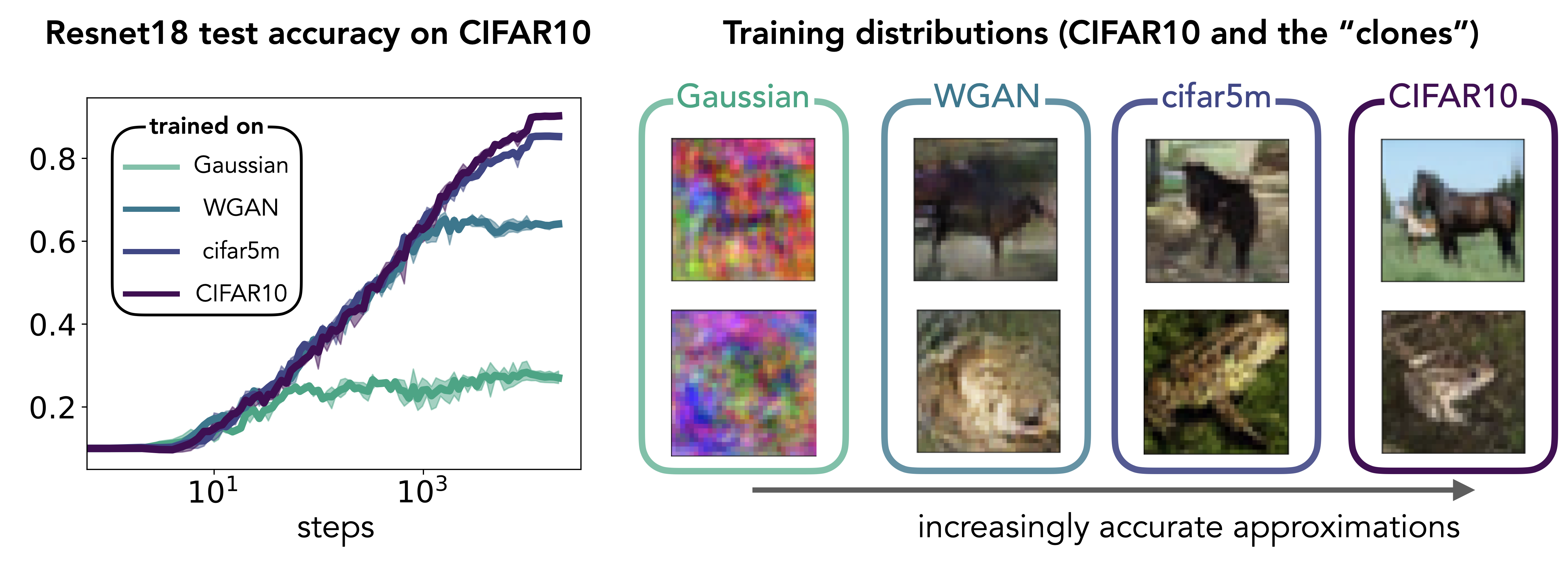
Figure 1: Distributional simplicity bias in neural networks. Test accuracy of a ResNet18 evaluated on CIFAR10 during training with SGD on four different training data sets: the standard CIFAR10 training set (dark blue), and three different “clones” of the training set. The images of the clones were drawn from a Gaussian mixture fitted to CIFAR10, a mixture of Wasserstein GAN (WGAN) (Arjovsky et al., 2017) fitted to CIFAR10, and the cifar5m data set of Nakkiran et al. (2021). The clones form a hierarchy of approximations to CIFAR10: while the Gaussian mixture captures only the first two moments of the inputs of each class correctly, the images in the WGAN and cifar5m data sets yield increasingly realistic images by capturing higher-order statistics. The ResNet18 trained on the Gaussian mixture has the same test accuracy on CIFAR10 as the baseline model, trained directly on CIFAR10, for the first 50 steps of SGD; the ResNet18 trained on cifar5m has the same error as the baseline model for about 2000 steps. This result suggests that the network trained on CIFAR10 discriminates the images using increasingly higher-order statistics during training (experimental details in Section 3).

We illustrate this idea in Figure 1, where we show the test accuracy of a ResNet18 (He et al., 2016) during training on CIFAR10 (dark blue line; details in Section 3). To understand which features of the data influence the ResNet, we trained the same network, starting from the same initial conditions, on a training set that was sampled from a mixture of Gaussians. Each Gaussian was fitted to one class of CIFAR10 and thus accurately captured the mean and covariance of the images in that class, but all the higher-order statistical information was lost. We show two example “images” sampled from the Gaussian mixture in Figure 1. We found that the test accuracy of the ResNet trained on the Gaussian mixture and evaluated on CIFAR10, (GM/CIFAR10 for short, green line) was the same as the accuracy of the ResNet trained directly on CIFAR10 for the first $\approx 50$ steps of SGD. In other words, the generalisation dynamics of the ResNet is governed by an effective distribution over the training data, which is well-approximated by a Gaussian mixture during the first 50 steps of SGD.

We also trained the same ResNet on two other approximations, or “clones”, of the CIFAR10 training set. The images in the WGAN clone were sampled from a mixture of ten Wasserstein GAN (Arjovsky et al., 2017), one for each class, while the images of the cifar5m clone provided by Nakkiran et al. (2021) were sampled from a large diffusion model and labelled using a pre-trained classifier (details in Section 3). The three clones – GM, WGAN, and cifar5m – constitute a hierarchy of increasingly accurate approximations of CIFAR10: while the Gaussians only capture the mean and covariance of each input class, the WGAN and cifar5m clones also capture higher-order statistics. CIFAR5M is a more accurate approximation than WGAN, as can be seen from the sharper example images in Figure 1 and from the final CIFAR10 accuracy of the ResNet trained on the two data sets, which is higher for cifar5m than for WGAN.

The key result of this experiment is that the CIFAR10 test accuracies of the ResNets during training on the different clones collapse: GM/CIFAR10 and CIFAR10/CIFAR10, the base model, achieve the same test accuracy for about 50 steps of SGD; WGAN/CIFAR10 matches the test accuracy of the base model for about 1000 steps, and cifar5m/CIFAR10 matches the base model for about 2000 steps. The effective training data distribution that governs the ResNet’s generalisation dynamics is therefore well-approximated by the GM, WGAN, and cifar5m datasets, for increasing amounts of time. We capture the essence of this experiment in the following conjecture:

Conjecture 1 (Distributional simplicity bias (DSB)).

A parametric model trained on a classification task using SGD discriminates its inputs using increasingly higher-order input statistics as training progresses.

In the remainder of this paper, we first demonstrate DSB in a solvable model of a single neuron trained on a synthetic data set (Section 2). We then demonstrate DSB in a variety of deep neural networks trained on CIFAR10, either from scratch or after pre-training on ImageNet (Section 3) Finally, we place DSB in the context of other simplicity biases, and highlight its implications for the principle of Gaussian universality in learning (Section 4).

1.1 Further related work

More simplicity biases in neural networks

Arpit et al. (2017) found empirically that two-layer MLP tend to fit the same patterns during the first epoch of training, and conjectured that such “easy examples” are learnt first by the network. Mangalam & Prabhu (2019) later found that deep networks trained on CIFAR10/100 first learn examples that can also be correctly classified by shallow models, and only then start to fit “harder” examples. Pérez et al. (2019) showed that the large majority of neural networks implementing Boolean functions with random weights have low descriptional complexity. Achille et al. (2019) highlighted the importance of the initial period of learning in models of biological and artificial learning by showing that certain deficits in the stimuli early during training, especially those that concern “low-level statistics”, cannot be reversed later during learning. Doimo et al. (2020) analysed ResNet152 trained on ImageNet and found that the distribution of neural representations across the layers clusters in a hierarchical fashion that mirrors the semantic hierarchy of the concepts, first separating broader – and hence, easier? – classes, before separating inputs between more fine-grained classes. However, neither Pérez et al. (2019) nor Doimo et al. (2020) considered the learning dynamics.

Complementary to simplicity biases, the implicit bias of SGD (Neyshabur et al., 2015) describes the mechanism by which a neural network trained using SGD “selects” one of the potentially many global minima in its loss landscape. In linear neural networks / matrix factorisation, this bias amounts to minimisation of a certain norm of the weights at the end of training (Brutzkus et al., 2018; Soudry et al., 2018; Gunasekar et al., 2017, 2018; Li et al., 2018; Ji & Telgarsky, 2019; Arora et al., 2019). These ideas have since been extended to non-linear two-layer neural networks (Lyu & Li, 2020; Ji & Telgarsky, 2020; Jin & Montúfar, 2020), see Vardi (2022) for a recent review. Here, we focus on the parts of the data that impact learning throughout training, rather than on the final weights.

Code availability  Code to reproduce our experiments and to include CIFAR10 clones in your experiments can be found on GitHub https://github.com/sgoldt/dist_inc_comp.

2 A toy model

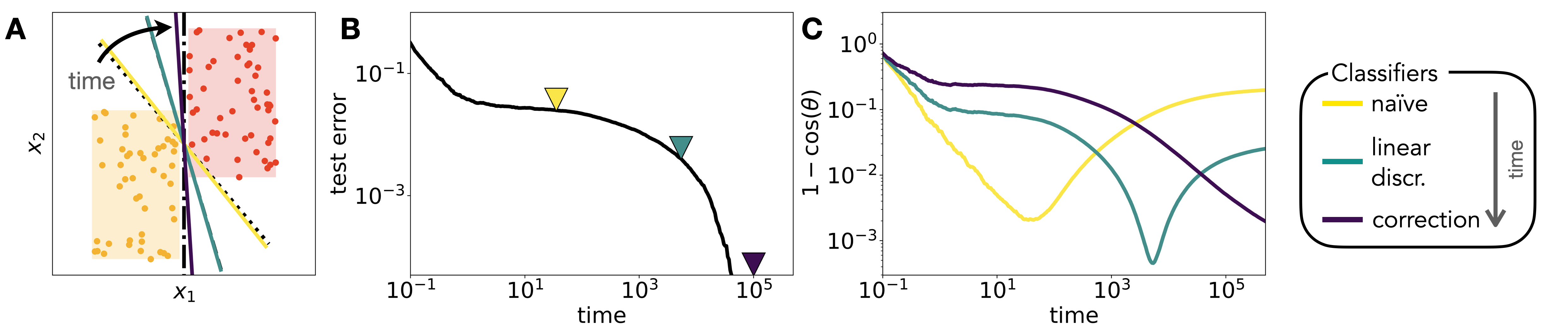
Figure 2: The decision boundary learnt by a perceptron takes increasingly higher-order statistics of the data into account during training  A: Inputs $x=(x_{i})$ are split into two classes (yellow vs red) which correspond to two rectangles in the $x_{1}-x_{2}$ plane; input components $x_{i>2}$ are sampled from a standard normal distribution. The coloured lines indicate the decision boundaries of a perceptron (1) trained on this task at different points during training, which are indicated with triangles in B. The black lines are given by the naïve classifier (Equation 4, dotted); the linear discriminant (Equation 8, dashed), and the oracle, which achieves perfect generalisation (dot-dashed).  B: Test error of the perceptron (1) during training on the rectangular data set.  C: Alignment of the weight vector of the perceptron (1) during training with the naïve classifier, the linear discriminant, and the non-Gaussian correction Equation 12. Smaller values indicate smaller angles $\theta$ between the weight vector and the respective classifier, and hence larger alignment.

We begin with an analysis of the simplest setup in which a classifier learns distributions of increasing complexity: a perceptron trained on a binary classification task.

Data set  We consider a simple “rectangular data set” where inputs $x={(x^{i})}_{i\leq D}$ are split in two equally probable classes, labelled $y=\pm 1$. The first two components $x_{1}$ and $x_{2}$ are drawn uniformly from one of the two rectangles shown in Figure 2A depending on their class. All other components are drawn i.i.d. from the standard normal distribution. This data set is linearly separable with an optimal decision boundary parallel to the $x_{1}$ axis, which we call the “oracle”.

Notation  We follow the convention of McCullagh (2018) and use the letter $\kappa$ for both moments and cumulants of the inputs. In particular, we denote the moments of the full input distribution $p(x)$ as $\kappa^{i}=\mathbb{E}\,x^{i}$, $\kappa^{ij}=\mathbb{E}\,x^{i}x^{j}$, while we denote class-wise averages will as $\kappa_{\pm}^{i}=\mathbb{E}\,_{\pm}x^{i}$, and so on. We set $\kappa^{i}=0$. For cumulants, we separate indices by commas: for example, $\kappa_{+}^{i,j}=\kappa_{+}^{ij}-\kappa_{+}^{i}\kappa_{+}^{j}$ is the covariance of the inputs in the class $y=+1$. The number of index partition gives the order of the cumulant, e.g. $\kappa^{i,j,k}$ is the third-order cumulant of the inputs. We summarise some useful facts on moments and cumulants in Section A.1.

Network  We learn this task using a single neuron, or perceptron, whose output is given by

$$\hat{y}=\sigma\left(\lambda\right),\qquad\lambda\equiv w_{i}x^{i}/\sqrt{D},$$ (1)

with weight vector $w=(w_{i})\in\mathbb{R}^{D}$ and activation function $\sigma:\mathbb{R}\to\mathbb{R}$. For concreteness, we consider the sigmoidal activation function in this section, although our argument is easily extended to other activations. We use superscript indices for inputs and lowerscript indices for weights, and imply a summation over any index repeated once as a superscript and once as a subscript. We use the square loss $\ell(\lambda,y)={(\sigma(\lambda)-y)}^{2}$ for training.

2.1 The stages of learning in the perceptron

We trained the perceptron on the rectangular data set with online learning, where we draw a new sample from the data distribution at each step of SGD, starting from Gaussian initial weights $w_{i}$ with variance 1. We show the test accuracy of the perceptron in Figure 2B. For the three points in time indicated by the coloured triangles, we plot the decision boundary of the perceptron at that time in Figure 2A (the decision boundary is the line at which the sign the perceptron output changes). Lighter colours correspond to earlier times, so a perceptron starting from random initial weights approaches the oracle from the left. In this section, we show that this series of classifiers takes increasingly higher-order statistics of the data set into account as training progresses.

We can gain analytical insight into the perceptron’s dynamics by studying the gradient flow

$$\dot{w}_{i}=\eta\mathbb{E}\,\left(\sigma(\lambda)-y\right)\sigma^{\prime}(\lambda)x^{i},$$ (2)

where $\mathbb{E}\,$ indicates an average over the data distribution and we fix the learning rate $\eta>0$. Upon expansion of the activation function around $\lambda=0$ as $\sigma(\lambda)=\sum_{k=0}^{\infty}\beta_{k}\lambda^{k}$, this becomes

$$\tau\dot{w}_{i}=\sum_{k=0}^{\infty}\mathbb{E}\,\lambda^{k}x^{i}(\gamma_{k}-\tilde{\beta}_{k+1}y),$$ (3)

where $\tau=1/\eta$, while $\tilde{\beta}_{k}$ and $\gamma_{k}$ are constants related to the Taylor expansion of $\sigma(\lambda)$ (see Section A.2). The gradient flow updates of the weight have thus two contributions: the first, proportional to $\gamma$, depends only on the inputs, while the second, proportional to $\tilde{\beta}$, depends on the product of inputs and their label. The interplay of this unsupervised and supervised terms is crucial during learning.

2.1.1 The first two moments of the inputs determine the initial learning dynamics

We start by considering gradient flow at zeroth order in the weights by truncating the sum in Equation 3 after a single term, which yields the anti-Hebbian updates $\tau\dot{w}^{(0)}_{i}=-\tilde{\beta}_{1}\mathbb{E}\,yx_{i}$ (recall that $\mathbb{E}\,x_{i}=0$). These dynamics show the typical run-away behaviour of Hebbian learning, where the norm of the weight vector grows indefinitely, but the weight converges in direction as

$$w^{(0)}_{i}\propto m^{i}\equiv\kappa_{+}^{i}-\kappa_{-}^{i},$$ (4)

which is the difference between the means of each class, $\kappa_{\pm}^{i}=\mathbb{E}\,_{\pm}x^{i}$. The decision boundary of the “naïve” classifier $m^{i}$ is drawn with a dashed black line in Figure 2A. Indeed, the full perceptron trained using online SGD initially converges in the direction of this naïve classifier, as can be seen from the overlap plot in Figure 2C, which peaks at the beginning of training (smaller values in the plot indicate smaller angles, and hence larger alignment).

At first order, the steady state of gradient flow is given by

$$\gamma_{1}\kappa^{ij}w^{(1)}_{i}=\tilde{\beta}_{1}m^{i}.$$ (5)

At first sight, it is not clear how the global second moment of the inputs, $\kappa^{ij}$, where we average over both classes simultaneously, can help the classifier separate the two classes. However, we can make progress by rewriting the second moment as (Bishop, 2006, sec. 4.1),

$$\kappa^{ij}=\kappa_{\mathrm{w}}^{i,j}/2+\kappa_{\mathrm{b}}^{i,j}/4,$$ (6)

with the between-class second moment $\kappa_{\mathrm{b}}^{i,j}=m^{i}m^{j}$ and the within-class second moment

$$\kappa_{\mathrm{w}}^{i,j}\equiv\underset{+}{\mathbb{E}}\,(x^{i}-\kappa_{+}^{i})(x^{j}-\kappa_{+}^{j})+\mathbb{E}\,_{-}(x^{i}-\kappa_{-}^{i})(x^{j}-\kappa_{-}^{j}).$$ (7)

Substituting these expressions into Equation 5 and noticing that $\kappa_{\mathrm{b}}^{i,j}w_{j}\propto m^{i}$, we find that at first order,

$$w^{\mathrm{(1)}}_{i}\propto{(\kappa_{\mathrm{w}})}_{i,j}m^{j}$$ (8)

is a solution of the gradient flow, where ${(\kappa_{\mathrm{w}})}_{i,j}$ is the matrix inverse of $\kappa_{\mathrm{w}}$. The classifier $w^{\mathrm{(1)}}_{i}$ is known as Fisher’s linear discriminant (Bishop, 2006, sec 4.1.). It is obtained by rotating the naïve classifier $m^{i}$ with the inverse of the within-class covariance. Its decision boundary is shown by the dashed black line in Figure 2A. The linear discriminant achieves a higher accuracy by exploiting the anisotropy of the covariances of each class. The decision boundary of the perceptron at time $\approx 8000$ is shown in the same plot with the green line; the overlap plot in Figure 2C also confirms that the perceptron weight moves towards the linear discriminant after initially aligning with the naïve classifier.

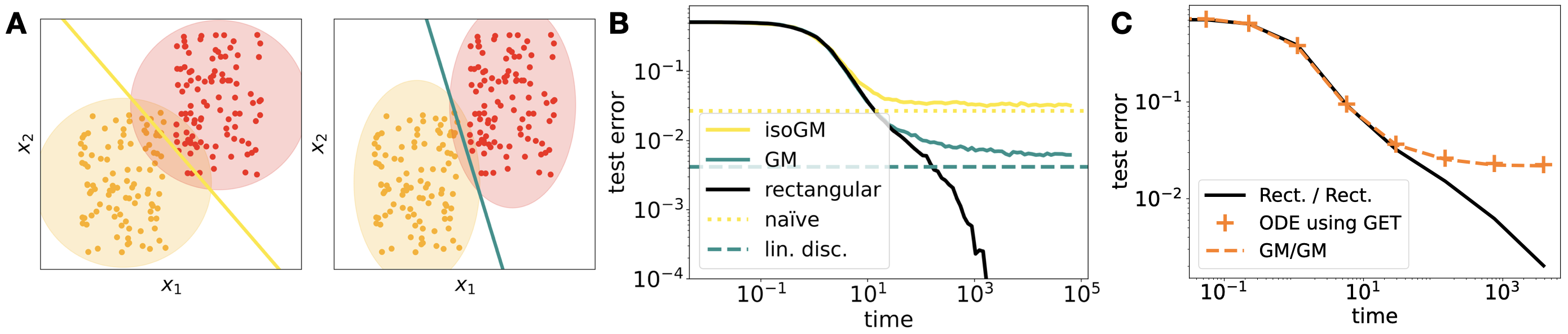
Figure 3: A perceptron learns distributions of increasing complexity  A: Gaussian mixture approximations of the rectangular data set, using only the correct mean (isotropic Gaussian, left) or the correct mean and covariance (right).  B: Test accuracy on the rectangular data set of a perceptron trained on the rectangular data set (black), as well as the isotropic (yellow) and full Gaussian mixture (green). Horizontal lines indicate the test accuracy of the naïve classifier, Equation 4 and the linear discriminant, Equation 8.  C: Test error evaluated on the rectangular data set of a perceptron trained on the rectangular data set (black) and as predicted by the dynamical equations of Refinetti et al. (2021) using the Gaussian equivalence theorem (dashed orange line). The Gaussian theory correctly captures the dynamics of a perceptron trained and evaluated on the Gaussian mixture (orange crosses). Parameters as in Figure 2.

2.1.2 Higher-order correlations bias the perceptron towards the oracle

The linear discriminant takes the first two moments of the inputs in each class into account, but it does not yield the optimal solution. How do higher orders of gradient flow drive the perceptron in the direction of the oracle? We show in Section A.2.3 that the second-order term does not add statistical information to the gradient flow. To compute the first non-Gaussian correction to the classifier, we analyse the GF up to third order in the weights, which includes the fourth-order moment of the inputs, $\kappa^{ijkl}$. To understand the impact of $\kappa^{ijkl}$ on the learnt classifier, we again decompose $\kappa^{ijkl}$ into a between-class fourth moment and a within-class fourth moment,

$$\kappa_{\mathrm{w}}^{ijkl}\equiv\underset{+}{\mathbb{E}}\,(x^{i}-\kappa_{+}^{i})\cdots(x^{l}-\kappa_{+}^{l})+\underset{-}{\mathbb{E}}\,(x^{i}-\kappa_{-}^{i})\cdots(x^{l}-\kappa_{-}^{l}).$$ (9)

We isolate the effect of the higher-order input statistics beyond the second moment by rewriting the within-class fourth moment as a within-class fourth cumulant $\kappa_{\mathrm{w}}^{i,j,k,l}$ and contributions from the mean and the second moment (green):

$$\kappa_{\mathrm{w}}^{ijkl}={\color[rgb]{0,0,0}\kappa_{\mathrm{w}}^{i,j,k,l}}+{\color[rgb]{0,0,0}2\kappa^{ij}\kappa^{kl}[3]}-{\color[rgb]{0,0,0}\frac{1}{2}m^{i}m^{j}\kappa^{kl}[6]}+{\color[rgb]{0,0,0}\frac{6}{16}m^{i}m^{j}m^{k}m^{l}}.$$ (10)

where we use the bracket notation like $[3]$ to denote the number of possible permutations of the indices. We can now rewrite the steady-state of the third-order GF as

$${\color[rgb]{0,0,0}c_{1}m^{i}}={\color[rgb]{0,0,0}c_{2}w_{j}\kappa_{\mathrm{w}}^{ij}}+{\color[rgb]{0,0,0}c_{3}w_{j}w_{k}w_{l}\kappa_{\mathrm{w}}^{i,j,k,l}}$$ (11)

where we separated the terms that capture the first or second moment of the inputs (green) from the term that captures higher-order input statistics (orange). If the data set was a mixture of Gaussians, $\kappa_{\mathrm{w}}^{i,j,k,l}$ would be zero. If we assume instead that the inputs in each class are weakly non-Gaussian, we can solve Equation 11 perturbatively by using $c_{3}$ as a small parameter. To zeroth order in $c_{3}$, Equation 11 has the same structure as the first-order GF in Equation 5 and we recover the linear discriminant, Equation 8. The first-order correction is given by

$$w_{i}^{*}\propto-{\color[rgb]{0,0,0}{(\kappa_{\mathrm{w}})}_{ij}}{\color[rgb]{0,0,0}\kappa_{\mathrm{w}}^{j,k,l,m}}{\color[rgb]{0,0,0}w^{(1)}_{k}w^{(1)}_{l}w^{(1)}_{m}}$$ (12)

and we plot the resulting classifier in violet in Figure 2A. The plot shows that the non-Gaussian correction pushes the weight in the direction of the oracle, improving performance. Note that if instead we computed the first-order correction with the vanilla fourth moment $k^{ijkl}$, the within-class fourth moment $k_{\mathrm{w}}^{ijkl}$, or the vanilla fourth cumulant $\kappa^{i,j,k,l}$, we do not obtain a correction that points in the right direction (dashed lines in Figure A.2).

2.2 A distribution-centric viewpoint

The perceptron did not learn an increasingly complex function during training – its decision boundary remains a straight line throughout training. Instead, we found that the direction of the weight vector, and hence its decision boundary, first only depends on the means of each class, Equation 4, then on their mean and covariance, Equation 8, and finally also on higher-order cumulants, Equation 12, yielding increasingly accurate predictors.

The decision boundary of the perceptron hence evolves as if the network was trained on increasingly accurate approximations of the rectangular data set like the ones shown in Figure 3A, which accurately capture the mean (isoGM, left), or the mean and covariance (GM, right) of each class, resp. To illustrate this point, in Figure 3D we show the test accuracy of a perceptron evaluated on the rectangular data set, but trained on the Gaussian clones of Figure 3A. Initially, all three perceptrons have the same test error, which means that they use only the information in the mean to classify samples. After the perceptron trained on isoGM converges to the naïve classifier, the perceptrons trained on GM and the rectangular data set have the same test error for a bit longer. The perceptron trained on the GM finally converges to the linear discriminant, while the perceptron trained on the rectangular data set converges to zero test error. Hence even a simple perceptron learns distributions of increasing complexity from its data, in the sense that it learns the optimal classifiers for increasingly accurate approximations of the true data distribution.

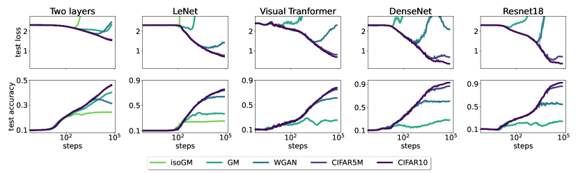
Figure 4: Neural networks trained on CIFAR10 learn distributions of increasingly complexity Test loss (top) and classification accuracy (bottom) of different neural networks evaluated on CIFAR10 during training on the various approximations of the CIFAR10 distribution described in Section 3. We show the mean (solid line) over three runs, starting from the same initial condition each time. The shaded areas indicate one standard deviation over the three runs. See Section B.2 for details on the architectures and training recipes.

2.3 The limits of Gaussian equivalence

The preceding analysis shows that even a simple perceptron goes beyond a Gaussian mixture approximation of its data, provided that higher-order cumulants of the inputs are task-relevant and improve the classifier. In other words, the perceptron breaks the Gaussian equivalence principle, or Gaussian universality, that stipulates that quantities like the test error of a neural network trained on realistic inputs can be exactly captured asymptotically by an appropriately chosen Gaussian model for the data. This idea allows to characterise the performance of random features and kernel regression (Liao & Couillet, 2018; Seddik et al., 2019; Bordelon et al., 2020; Mei & Montanari, 2021), and has also been used to analyse two-layer neural networks (Goldt et al., 2020; Hu & Lu, 2022; Loureiro et al., 2021a; Goldt et al., 2022; Gerace et al., 2022) and autoencoders (Refinetti & Goldt, 2022) trained on realistic synthetic data.

1 suggests that Gaussian equivalence can always be applied to the early period of training a neural network before the higher-order cumulants affect the generalisation dynamics. We illustrate this phenomenon in Figure 3C, where we show the test error of a perceptron trained on the rectangular data set as predicted by Gaussian equivalence and the dynamical equations of Refinetti et al. (2021) (orange crosses). The theory accurately predicts the test error of a perceptron trained and evaluated on the Gaussian mixture (orange dashed line). At the beginning of training, the theory also matches the test accuracy of a perceptron trained and evaluated on the rectangular data (black line), but the agreement breaks down at time $t\approx 10$. Ingrosso & Goldt (2022) recently made a similar observation for two-layer networks trained on a simple model of images.

3 Learning increasingly complex distributions on CIFAR10

The gradient flow analysis of the perceptron from Section 2 cannot be readily generalised even to two-layer networks. However, the distribution-centric point of view of Section 2.2 offers a way to test 1 in more complex neural networks by constructing a hierarchy of approximations to a given data distribution, similar to the Gaussian approximations of Figure 3.

A hierarchy of approximations to CIFAR10  Our goal is to construct a series of approximations to CIFAR10 which capture increasingly higher moments. To have inputs with the correct mean per class, we sampled a mixture with one isotropic Gaussian for each class (isoGP). Inputs sampled from a mixture of ten Gaussians (GM), each one fitted to one class of CIFAR10, have the correct mean and covariance per class, but leave all higher-order cumulants zero. Ideally, we’d like to extend this scheme to distributions where the first $m$ cumulants are specified, while cumulants of order greater than $m$ are zero. Unfortunately, there are no such distributions; on a technical level, the cumulant generating function of a distribution, Equation A.4, has either one term, two terms, corresponding to a Gaussian, or infinitely many terms (Lukacs, 1970, thm. 7.3.5). We therefore turned to generative neural networks for approximations beyond the Gaussian mixture. For the WGAN data set, we sampled images from a mixture of ten deep convolutional GAN (Radford et al., 2016), each one trained on one class of CIFAR10. We ensured that samples from each WGAN have the same mean and covariance as CIFAR10 images; as we detail in Section B.1, the key to obtaining “consistent” GANs was using the improved Wasserstein GAN algorithm (Arjovsky et al., 2017; Gulrajani et al., 2017). We finally also used the cifar5m data set provided by Nakkiran et al. (2021), who sampled images from the denoising diffusion probabilistic model of Ho et al. (2020) and labelled them using a Big-Transfer model (Kolesnikov et al., 2020). We show one example image for each class in Figure B.1.

Methods  We trained neural networks with different architectures on both CIFAR10 and CIFAR10 clones like the Gaussian mixture, which we describe in detail below. Networks were trained three times starting from the same standard initial conditions given by pytorch (Paszke et al., 2019), varying only the random data augmentations and the order in which samples were shown to the network. Unless otherwise noted, we trained all models using vanilla SGD with learning rate 0.005, cosine learning rate schedule (Loshchilov & Hutter, 2017), weight decay $5\mathrm{e}^{-4}$, momentum 0.9, mini-batch size 128, for 200 epochs (see Section B.2 for details).

Results  We show the test loss and test accuracy of all the models evaluated on CIFAR10 during training on the different clones in Figure 4. We found that both a fully-connected two-layer network and the convolutional LeNet of LeCun et al. (1998), learnt distributions of increasing complexity. Interestingly, a two-layer network trained on GM performs better on CIFAR10 in the long run than the same network trained on WGAN. This suggests that for a simple fully-connected network, having precise first and second moments is more important than the higher-order cumulants generated by the convolutions of the WGAN. The trend is already reversed in LeNet, which has two convolutional layers. We also found a distributional simplicity bias in DenseNet121 (Huang et al., 2017) and ResNet18 (He et al., 2016), which are deep convolutional networks with residual connections, batch-norm, etc. We also tested a visual transformer (ViT) (Dosovitskiy et al., 2021), which is an interesting alternative architecture since it does not use convolutions, but instead treats the image as a sequence of patches which are processed using self-attention (Vaswani et al., 2017). Despite these differences, we found that the ViT also learns distributions of increasing complexity on CIFAR10.

3.1 Pre-trained neural networks learn distributions of increasing complexity, too

One might argue that drawing the initial weights of the networks i.i.d. from the uniform distribution biases the network towards lower-order input statistics early during training due to the effect of the central limit theorem in fully-connected layers. We investigated this by repeating the experiment with a ResNet18 that was pre-trained on ImageNet, as provided by the timm library (Wightman, 2019). We re-trained the entire network end-to-end, following the same protocol as above. While we found that pre-training improved the final accuracy of the model and significantly improved the training speed, the pre-trained ResNet also learnt distributions of increasing complexity, cf. Figure 5A, even though its initial weights were now large and strongly correlated.

This observation begs the question of what the network transferred from ImageNet to CIFAR10, since the generalisation dynamics of the pre-trained and the randomly initialised ResNet18 follow the same trend, albeit at different speeds. While we leave a more detailed analysis of transfer learning using clones to future work, we note that several papers have suggested that some of the benefits of pre-training could be ascribed to finding a good initialisation, rather than the transfer of “concepts”, both in computer vision (Maennel et al., 2020; Kataoka et al., 2020) and in natural language processing (Krishna et al., 2021).

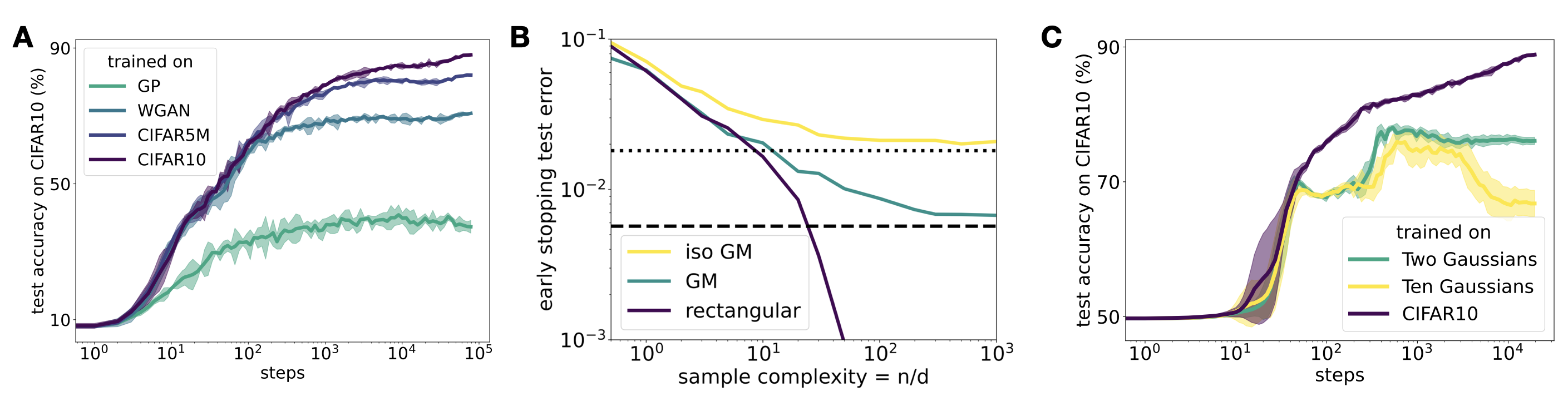
Figure 5: A: Pre-trained networks learn distributions of increasing complexity, too. Test accuracy of a ResNet18 under the same protocol as in Figure 4, but this time starting from weights that were pre-trained on ImageNet. B: Distributional simplicity bias on finite data sets Early-stopping test-accuracy of a perceptron trained using SGD on a finite number of $n$ samples, drawn from the rectangular data set of Figure 2A (blue) and matching Gaussian mixtures with isotropic and anisotropic covariance (yellow and green, resp.). The dotted and dashed horizontal line indicate the performance of the naïve and linear classifier, resp. C: How many Gaussians do you need? Test accuracy of LeNet evaluated on a coarse-grained CIFAR10 task with two classes during training on three different input distributions: the CIFAR10 training images, a mixture of two Gaussians, one for all the images in each class with the right mean and covariance, and a mixture of ten Gaussians, one per class with the right mean and covariance.

4 Discussion

The distributional simplicity bias is related to the idea of learning functions of increasing complexity, but one doesn’t imply the other directly. Any parametric model $f(x;\theta)$ that admits a Taylor-expansion around its initial parameters $\theta_{0}$ is linear in its parameters $\theta$ at the beginning of training, then quadratic, etc. We saw explicitly for the perceptron how this increasing degree of the effective model that is being optimised makes the model first susceptible to class-wise means, then class-wise covariances, etc. However, this expansion of $f(x;\theta)$ breaks down early during training for neural networks in the feature learning regime (Chizat et al., 2019). Yet we see that the performance of cifar5m/CIFAR10 and CIFAR10/CIFAR10 agree for almost the entire training.

A second important distinction between DSB and the Taylor-expansion point of view is the way in which networks are influenced by higher-order cumulants. Once the effective model that is being optimised has degree three or higher, it should behave differently on two data sets that have different third-order cumulants. While we ensured that the class-wise covariances were close to each other across the different data sets, it is reasonable to assume that already the third- or fourth-order cumulants of WGAN or cifar5m images are not exactly equal to each other or corresponding CIFAR10 cumulants. If the generalisation dynamics of the neural network depended on the full third-order cumulants of each class, the test accuracy of WGAN/CIFAR10 and cifar5m/CIFAR10 should diverge quickly after they separate from the test accuracy of GM/CIFAR10. Instead, the curves stay together for much longer, suggesting that only a part of the cumulant, for example its low-rank decomposition (Kolda & Bader, 2009), is relevant for the generalisation dynamics at that stage. Investigating in more detail how higher-order cumulants affect the generalisation dynamics of neural networks is an important direction for further work.

Learning increasingly complex distributions from finite data sets  Varying the data set size offers a complementary view on the distributional simplicity bias. We explored this by training a perceptron (1) on a fixed data set with $n$ samples drawn from the rectangular data set of Section 2 using online SGD. The early-stopping test accuracy plotted in Figure 5B shows that the perceptron also learns distributions of increasing complexity as a function of sample complexity – for a small number of samples, the perceptron will achieve the same test error on the rectangular data set after training on the rectangular data (violet) or on the Gaussian mixture approximation (green). We also note that the power-law exponent of the test accuracy as a function of sample complexity changes roughly when the Gaussian approximation breaks down. A theoretical treatment of this effect would requires advanced tools such as dynamical mean-field theory (Mignacco et al., 2020a, b), which leave as an intriguing avenue for further work.

How many distributions do you need in your mixture?  We modelled inputs using mixtures with one distribution per class, following the structure of the gradient flow equations. We could obtain a more detailed model of the inputs by modelling each class using a mixture of distributions. We compared the two approaches for the two-layer network and the LeNet, which both achieve good performance on GM/CIFAR10. We trained the networks on a coarse-grained version of CIFAR10 (CIFAR10c): (cat, deer, dog, frog, horse) vs. (plane, car, bird, ship, truck). We also trained the same network on two different clones of CIFAR10c: a mixture of two Gaussians, one for each superclass, and a mixture of ten Gaussians, one for each input class of CIFAR10, with binary labels according to CIFAR10c. We trained a LeNet on CIFAR10c and the two clones and found that LeNets trained on either clone had the same test accuracy on CIFAR10c as the network trained on CIFAR10c for the same number of SGD steps, cf. Figure 5C. This suggests that the network trained on CIFAR10 started to look at higher-order cumulants at that point, rather than at a mixture with more distributions. However, asymptotically, the more detailed input distribution with ten Gaussians yields better results. This observation is in line with the results of Loureiro et al. (2021b), who compared two-Gaussian to ten-Gaussian approximations for a binary classification task on MNIST and FashionMNIST and found that the ten-Gaussian approximation gave a more precise prediction of the asymptotic error of batch gradient descent on a perceptron (cf. their fig. 10).

5 Concluding perspectives

We have found a distributional simplicity bias in an analytically solvable toy model of a neural network, and in a range of deep networks trained on CIFAR10. Our focus was on evaluating their test accuracy, which is their most important characteristic in practice. To gain a better understanding of DSB, it will be key to analyse the networks using more fine-grained measures of generalisation, for example distributional generalisation (Nakkiran & Bansal, 2020), and to look at the information processing along the layers of the network. Different parts of the networks are influenced by different statistics of their inputs; this point was made recently by Fischer et al. (2022), who used field-theoretic methods to show that Gaussian correlations dominate the information processing of internal layers, while the input layers are also sensitive to higher-order correlations. This finding motivates studying the structure of the internal representations of inputs across layers for networks trained on the different clones (Alain & Bengio, 2017; Bau et al., 2017; Raghu et al., 2017; Ansuini et al., 2019; Doimo et al., 2020).

The key challenge for future work is to clarify the range of validity of 1 by testing it on other data sets, like ImageNet (Deng et al., 2009) with its rich semantic structure of hierarchical classes. These experiments require training generative models for each of the 1000 classes of ImageNet, so we leave this to future work. While we have focused on correlations at the level of pixels in each image, one could also explore different statistical “clones” based on correlations between patches of pixels, or correlations in a different feature space. Likewise, it would be interesting to consider different data modalities, such as natural language. In the meantime, we hope that the hierarchy of approximations to CIFAR10 will be a useful tool for further investigations on the role of data structure in learning with neural networks.

Appendix A Details on the theoretical analysis

In this section, we summarise some useful facts and identities about moments and cumulants in high dimensions, before giving a detailed derivation of the theoretical results on the perceptron discussed in Section 2.1.

A.1 Moments and cumulants in high dimensions

This section summarises some basic results and identities on moments and cumulants of high-dimensional random variables, using the notation of McCullagh (2018). We consider $D$-dimensional random variables $x$ with components $x^{1},x^{2},\ldots,x^{D}$. We will use the superscript notation exclusively to denote the components of $x$, which will allow us to make heavy use of index notation and in particular, of the Einstein summation convention. Hence we will write quadratic or cubic forms as

$$a_{ij}x^{i}x^{j}=\sum_{i,j=1}^{p}a_{ij}x^{i}x^{j},\qquad a_{ijk}x^{i}x^{j}x^{k}=\sum_{i,j,k=1}^{p}a_{ijk}x^{i}x^{j}x^{k},$$ (A.1)

where $a_{ij}$ are arrays of constants. For the sake of simplicity, and without loss of generality, we take all multiply-indexed arrays to be symmetric under index permutation

We can write the moments of $x$ as

$$\kappa^{i}=\mathbb{E}\,x^{i},\quad\kappa^{ij}=\mathbb{E}\,x^{i}x^{j},\quad\kappa^{ijk}=\mathbb{E}\,x^{i}x^{j}x^{k},\quad\mathrm{etc.}$$ (A.2)

These moments are also defined implicitly by the moment-generating function

$$M_{X}(\xi)=\mathbb{E}\,\exp(\xi_{i}x^{i})=1+\xi_{i}\kappa^{i}+\xi_{i}\xi_{j}\kappa^{ij}/2!+\xi_{i}\xi_{j}\xi_{k}\kappa^{ijk}/3!+\ldots$$ (A.3)

as the partial derivatives of $M_{X}(\xi)$ evaluated at $\xi=0$. The cumulants are most easily defined via the cumulant generating function

$$K_{x}(\xi)\equiv\log M_{x}(\xi)$$ (A.4)

which can similarly be expanded to yield the cumulants:

$$K_{x}(\xi)=\xi_{i}\kappa^{i}+\xi_{i}\xi_{j}\kappa^{i,j}/2!+\xi_{i}\xi_{j}\xi_{k}\kappa^{i,j,k}/3!+\ldots$$ (A.5)

Note that we use the same letter $\kappa$ to denote both cumulants and moments, the difference being the commas, which are considered as separators for the cumulant indices.

We can relate cumulants and moments by expanding the $\log$ of the definition of $K_{x}(\xi)$ (A.4) and comparing terms to the expansion Equation A.5. Moments can be written in terms of cumulants as

$$\kappa^{ij} =\kappa^{i,j}+\kappa^{i}\kappa^{j},$$ (A.6)

$$\kappa^{ijk} =\kappa^{i,j,k}+(\kappa^{i}\kappa^{j,k}+\kappa^{j}\kappa^{i,k}+\kappa^{k}\kappa^{i,j})+\kappa^{i}\kappa^{j}\kappa^{k}$$

$$=\kappa^{i,j,k}+\kappa^{i}\kappa^{j,k}[3]+\kappa^{i}\kappa^{j}\kappa^{k},$$

where we introduced the bracket notation $[3]$ to denote all the partitions of the indices $i,j,k$ into two groups: $(i,jk),(j,ik)$ and $(k,ij)$.

Similarly, we can derive expressions for the cumulants in terms of the moments by inverting the equations above. We find that

$$\kappa^{i,j} =\kappa^{ij}-\kappa^{i}\kappa^{j},$$ (A.7)

$$\kappa^{i,j,k} =\kappa^{ijk}-\kappa^{i}\kappa^{jk}[3]+2\kappa^{i}\kappa^{j}\kappa^{k}.$$

A.2 Detailed calculations for the perceptron

We start again from the gradient flow equation, Equation 2. Expanding the activation function as $\sigma(\lambda)=\sum_{k=0}^{\infty}\beta_{k}\lambda^{k}$ yields $\sigma^{\prime}(\lambda)=\sum_{k=0}^{\infty}\tilde{\beta}_{k+1}\lambda^{k}$ for the derivative with $\tilde{\beta}_{k}=k\beta_{k}=k\,\sigma^{(k)}(\lambda)|_{\lambda=0}$. The gradient flow Equation 2 up to order $K$ then becomes

$$\tau\dot{w}_{i}=\sum_{k=0}^{K}\mathbb{E}\,\lambda^{k}x^{i}(\gamma_{k}-\tilde{\beta}_{k+1}y),$$ (A.8)

where $\tau=1/\eta$, and $\sigma^{(k)}$ denotes the $k$th derivative, while $\gamma_{k}$ is a linear combination of $\beta_{k}$: $\gamma_{0}=\beta_{0}\beta_{1},\gamma_{1}=\beta_{1}^{2}+2\beta_{0}\beta_{2}$, etc.

A.2.1 Zeroth order: the naïve classifier

For $K=0$, we have $\tau\dot{w}^{(0)}_{i}=x_{i}\gamma_{0}-\tilde{\beta}_{1}yx_{i}$. Under expectation, the first term goes to zero, and we are left with the anti-Hebbian updates $\tau\dot{w}^{(0)}_{i}=-\tilde{\beta}_{1}\mathbb{E}\,yx_{i}$, which show the typical run-away behaviour of Hebbian learning, while the weight converges in direction to

$$w^{(0)}_{i}\propto m^{i}\equiv\kappa_{+}^{i}-\kappa_{i}^{i},$$ (A.9)

which is the difference between the mean of each class.

A.2.2 First order: the linear discriminant

For $K\leq 1$, we find that after averaging

$$\begin{split}\tau\dot{w}_{i}=&-\tilde{\beta}_{1}(\kappa_{+}^{i}-\kappa_{-}^{i})\\ &+w_{j}(\gamma_{1}\kappa^{ij}-\tilde{\beta}_{2}(\kappa_{+}^{ij}-\kappa_{-}^{ij}))\end{split}$$ (A.10)

where $\kappa^{ij}$ is the second moment of the inputs, while $\kappa_{\pm}^{ij}$ are the second moments for each class (cf. Section 2). Note that in the rectangular data set, both classes have the same the same covariance matrix, $\kappa_{+}^{i,j}-\kappa_{-}^{i,j}=0$, which makes the $\tilde{\beta}_{2}$ term vanish. A pattern emerges in the updates: while the unsupervised terms $\propto\gamma$ contain moments of the inputs averaged over the whole distribution $p(x)$, the supervised terms ($\propto\beta$) depend on the class-wise differences between moments.

In the steady state, we find that

$$\gamma_{1}\kappa^{ij}w_{j}=\tilde{\beta}_{1}m^{i}$$ (A.11)

At first sight, it is not clear how the global second-moment of the inputs $\kappa^{ij}$, which averages over both classes, can help with discriminating the two classes. However, we can make progress by rewriting the total second moment of the inputs as

$$\kappa^{ij}=\kappa^{i,j}=\kappa_{\mathrm{w}}^{i,j}/2+\kappa_{\mathrm{b}}^{i,j}/4,$$ (A.12)

where we introduced the between-class covariance (Bishop, 2006, sec. 4.1),

$$\kappa_{\mathrm{b}}^{ij}\equiv(\kappa_{+}^{i}-\kappa_{-}^{i})(\kappa_{+}^{j}-\kappa_{-}^{j})=m^{i}m^{j},$$ (A.13)

and the within-class covariance,

$$\begin{split}\kappa_{\mathrm{w}}^{i,j}&\equiv\underset{+}{\mathbb{E}}\,(x^{i}-\kappa_{+}^{i})(x^{j}-\kappa_{+}^{j})+\mathbb{E}\,_{-}(x^{i}-\kappa_{-}^{i})(x^{j}-\kappa_{-}^{j})\\ &=\kappa_{+}^{ij}-2\kappa_{+}^{i}\kappa_{+}^{j}\end{split}$$ (A.14)

Substituting these expressions into Equation A.11 and noticing that $\kappa_{\mathrm{b}}^{i,j}w_{j}\propto m^{i}$, we find that the linear discriminant

$$w^{\mathrm{(1)}}_{i}\propto{(\kappa_{\mathrm{w}})}_{ij}m^{j}$$ (A.15)

is a solution to the steady-state of gradient flow up to first order. This classifier performs better than the naïve classifier $w_{i}\propto m^{i}$, since rotating the naïve classifier with the inverse of the within-class covariance brings the classifier closer to the oracle (cf. Figure 2).

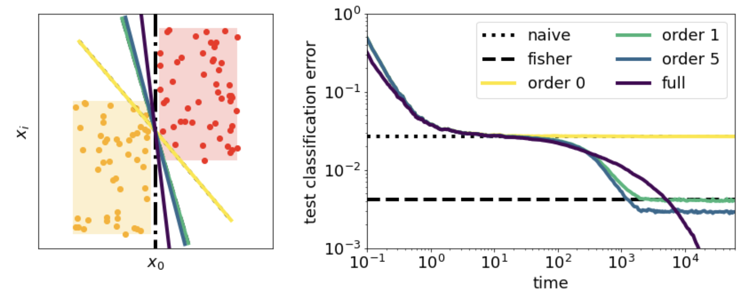
Figure A.1: Evolution of truncated gradient flow. Left: Rectangular data set together with the weight vectors obtained from integrating the truncated gradient flow; colours correspond to the orders indicated in the legend of the right plot. Right: Evolution of the test accuracy of the perceptron when the weight follows the truncated gradient flow at the given order. Horizontal lines indicate the test accuracy of the naïve classifier, Equation 4, and of the linear discriminant, Equation 8. Setup and parameters like in Figure 2.

A.2.3 The second order does not yield new statistical information

For $K\leq 2$, the steady state of the gradient flow is

$$\tilde{\beta}_{1}(\kappa_{+}^{i}-\kappa_{-}^{i})=w_{j}\left(\gamma_{1}\kappa^{ij}-\tilde{\beta}_{2}(\kappa_{+}^{ij}-\kappa_{-}^{ij})\right)+w_{j}w_{k}\left(\gamma_{2}\kappa^{ijk}-\tilde{\beta}_{3}(\kappa_{+}^{ijk}-\kappa_{-}^{ijk})\right)$$ (A.16)

While the third-order moment $\kappa^{ijk}=0$ due to symmetry, the difference between class-wise third-order moments $\kappa_{+}^{ijk}-\kappa_{-}^{ijk}$ is not. We can however express this difference in terms of global quantities, i.e. those pertaining to the full input distribution $p(x)$, by using the identities

$$\kappa_{\pm}^{i}=\pm\,m^{i}/2\mbox{\quad and\quad}\kappa_{\pm}^{ij}=\kappa^{ij}.$$ (A.17)

The latter follows from the fact that by construction, the two cumulants $\kappa_{\pm}^{i,j}$ are equal to each other. We find that

$$\kappa_{+}^{ijk}-\kappa_{-}^{ijk}=m^{i}\kappa^{jk}[3]-\frac{1}{2}m^{i}m^{j}m^{k},$$ (A.18)

where we use the bracket notation $m^{i}\kappa^{jk}[3]$ to denote all the permutations of the indices, cf. Equation A.6. The steady state hence becomes

$$\tilde{\beta}_{1}m^{i}=\gamma_{1}w_{j}\kappa^{ij}+\tilde{\beta}_{3}w_{j}w_{k}\left(m^{i}\kappa^{jk}[3]-\frac{1}{2}m^{i}m^{j}m^{k}\right).$$ (A.19)

Upon contracting the terms proportional to $\tilde{\beta}_{3}$, we see that these terms are all proportional either to $m^{i}$ or to $w_{j}\kappa^{ij}$. We showed above that the linear discriminant is a solution to this equation, so going to second order does not bring any additional statistical information that would change, or even improve, the classifier.

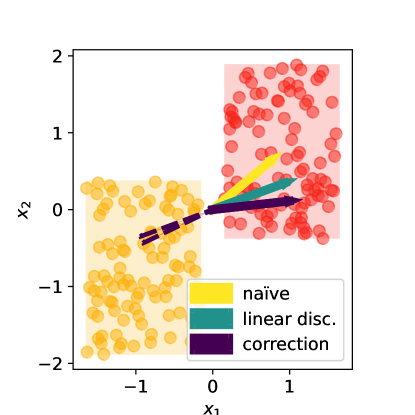
Figure A.2: Non-Gaussian correction to the linear discriminant drives the perceptron towards the oracle. Rectangular data set together with the naïve classifier, Equation A.9, and the linear discriminant, Equation 8. The latter only takes the Gaussian statistics of each class into account and does not yield the optimal classifier, which would be parallel to the $x_{1}$-axis. We show that the first non-Gaussian correction, Equation A.28, which we compute perturbatively in Section A.2.4, drives the classifier towards this oracle. The dashed violet lines show “corrections” that are computed with the wrong fourth-order tensor, as discussed after Equation 12.

A.2.4 Third order: the first non-Gaussian correction to the linear discriminant

At third order in the weights however, the non-Gaussian statistics start to impact the dynamics. The steady state is given by

$$\tilde{\beta}_{1}m^{i}=\gamma_{1}w_{j}\kappa^{ij}+\tilde{\beta}_{3}w_{j}w_{k}\left(m^{i}\kappa^{jk}[3]-\frac{1}{2}m^{i}m^{j}m^{k}\right)+\gamma_{3}w_{j}w_{k}w_{l}\kappa^{ijkl}$$ (A.20)

since the local terms cancel out, $\kappa_{+}^{ijkl}-\kappa_{-}^{ijkl}=0$. Our goal is now to understand how the fourth-order moment $\kappa^{ijkl}$ changes the weight vector in the steady state. Following the logic of the analysis that led us to the linear discriminant, we first decompose the fourth-order moment into a within-class fourth-order moment $\kappa_{\mathrm{w}}^{ijkl}$, and contributions from lower orders:

$$\kappa^{ijkl}=\frac{1}{2}\kappa_{\mathrm{w}}^{ijkl}+\frac{1}{8}\kappa_{\mathrm{w}}^{ij}m^{k}m^{l}[6]+\frac{1}{16}m^{i}m^{j}m^{k}m^{l},$$ (A.21)

where

$$\kappa_{\mathrm{w}}^{ijkl}\equiv\underset{+}{\mathbb{E}}\,(x^{i}-\kappa_{+}^{i})(x^{j}-\kappa_{+}^{j})(x^{k}-\kappa_{+}^{k})(x^{l}-\kappa_{+}^{l})+\underset{-}{\mathbb{E}}\,(x^{i}-\kappa_{-}^{i})\cdots(x^{l}-\kappa_{-}^{l}).$$ (A.22)

After contraction with the weights, the second and third term in Equation A.21 also appear in the equation that yields the linear classifier, so they do not change the direction of the final classifier. Instead, we need to focus on the within-class fourth moment. If the data set was a mixture of Gaussians, instead of a mixture of rectangles, the perceptron would converge to the linear discriminant at any order of gradient flow. So while $\kappa_{\mathrm{w}}^{ijkl}$ would be non-zero for the mixture of Gaussians, it would not change the direction of the classifier. We have hence to split $\kappa_{\mathrm{w}}^{ijkl}$ into a Gaussian and a non-Gaussian part,

$$\kappa_{\mathrm{w}}^{ijkl}=\kappa_{\mathrm{w}}^{i,j,k,l}+\kappa_{\mathrm{w},G}^{ijkl},$$ (A.23)

where $\kappa_{\mathrm{w},G}^{ijkl}$ is defined as

$$\kappa_{\mathrm{w,G}}^{ijkl} \equiv\underset{+,\mathrm{G}}{\mathbb{E}\,}(x^{i}-\kappa_{+}^{i})\cdots(x^{l}-\kappa_{+}^{l})+\underset{-,\mathrm{G}}{\mathbb{E}\,}(x^{i}-\kappa_{-}^{i})\cdots(x^{l}-\kappa_{-}^{l})$$ (A.24)

$$=2\kappa^{ij}\kappa^{kl}[3]-\frac{1}{2}m^{i}m^{j}\kappa^{kl}[6]+\frac{6}{16}m^{i}m^{j}m^{k}m^{l}$$ (A.25)

and $\underset{\pm,G}{\mathbb{E}\,}$ denotes the average over a Gaussian distribution with the same mean and covariance as the rectangular distribution corresponding to $y=\pm 1$.

Inserting these expressions into the steady-state gradient flow equation Equation A.20, we find

$$c_{1}(w)m^{i}=c_{2}(w)w_{j}\kappa_{\mathrm{w}}^{ij}+c_{3}(w)w_{j}w_{k}w_{l}\kappa_{\mathrm{w}}^{i,j,k,l},$$ (A.26)

where the constants $c_{1},c_{2},c_{3}$ depend on the weight through the contractions. For a fixed $c_{1},c_{2},c_{3}$, we can solve the equation. To determine the direction of the weight, this is enough; for an exact solution, one would need to substitute the solution for $w$ with fixed constants back into Equation A.26 and find a self-consistent equation for the constants.

Here, we are only interested in understanding the direction of the weight vector, so we simply fix the constants. We further assume that the data are only weakly non-Gaussian, making $c_{3}$ a small parameter that allows us to solve the cubic equation Equation A.26 perturbatively. By expanding the weight as

$$w_{i}=w_{i}^{(1)}+c_{3}w_{i}^{(2)}+\mathcal{O}(c_{3}^{2}),$$ (A.27)

we have that $w^{(1)}\propto{(\kappa_{\mathrm{w}})}_{ij}m^{j}$ is the linear discriminant by construction. The first-order correction is then given by

$$w_{i}^{(2)}\propto-{(\kappa_{\mathrm{w}})}_{ij}\kappa_{\mathrm{w}}^{j,k,l,m}w^{(1)}_{k}w^{(1)}_{l}w^{(1)}_{m},$$ (A.28)

which we plot in Figure A.2 together with the naïve classifier and the linear discriminant, $w^{(1)}$. From the plot, it becomes clear that this first non-Gaussian correction to the classifier pushes the weight in the direction of the oracle.

Note that if we instead compute the first-order correction with the full fourth moment $\kappa^{ijkl}$ or even the within-class fourth moment $\kappa_{\mathrm{w}}^{ijkl}$, we obtain corrections that point roughly in the opposite direction of the linear discriminant (dashed lines in Figure A.2). If instead we use the global fourth-order cumulant $\kappa^{i,j,k,l}$ to compute the correction, we obtain the linear discriminant.

Appendix B Details on the CIFAR10 experiments

B.1 Synthetic data sets

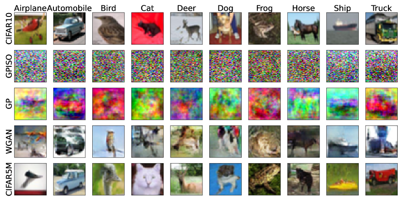
Figure B.1: Approximations of CIFAR10 of increasing complexity We show a randomly drawn example image of each of the 10 classes of CIFAR10 (Krizhevsky et al., 2009) in the top row. Below, we show an image drawn at random from each class of four different approximations of CIFAR10: a mixture of one isotropic Gaussian per class (“isoGM”), a mixture of one Gaussians per class with the correct mean and covariance (“GM”), a mixture of one improved Wasserstein GAN (Arjovsky et al., 2017; Gulrajani et al., 2017) per class. We also used the cifar5m data set of Nakkiran et al. (2021), who sampled images from a denoising diffusion model (Ho et al., 2020) and labelled it with a BigTransfer model (Kolesnikov et al., 2020).

We constructed several approximations to the original CIFAR10 data set (Krizhevsky et al., 2009) for the experiments described in Section 3. Here, we give details on how we sampled these data sets. The code for sampling them can be found on the GitHub repository accompanying the paper.

Gaussian mixtures

We constructed two Gaussian mixtures to approximate CIFAR10. For each colour channel, we sampled from a mixture of 10 Gaussians, with one Gaussian for each class. The Gaussians had the correct mean per class. For the isotropic Gaussian (“isoGM”), the covariance for each class was the identity matrix times the class-wise standard deviation of the inputs. For the correct second-order approximation (“GM”), we sampled from a mixture of one Gaussian per class with the correct mean and covariance. We constrained the values of the Gaussian samples to be in the range $[0,255]$ by setting all negative values to 0 and all values larger than 255 to 255.

WGAN

We sampled images from a mixture of deep convolutional GANs, using the architecture of Radford et al. (2016). Each GAN was trained on a single class of the CIFAR10 training set. Interestingly, we found that GANs trained with the “vanilla” algorithm (Goodfellow et al., 2014) yield statistically inconsistent images: while visually appealing, the images do not have the right covariance, and sometimes not even the right mean. We therefore resorted to training the GANs using the improved Wasserstein GAN algorithm (Arjovsky et al., 2017; Gulrajani et al., 2017). We show how the mean and the covariance of the samples drawn from GANs trained in this way do converge towards the mean and covariance of the CIFAR10 images, see Figure B.2. These results are in line with an earlier theoretical study by Cho & Suh (2019) who showed that a linear Wasserstein GAN will learn the principal components of its data. We validated the data set using a Resnet18 (He et al., 2016) that we trained to 94% test accuracy on CIFAR10 following the recipe of van Amersfoort (2021). This Resnet18 classified the WGAN data set with an accuracy of 80%.

cifar5m

The cifar5m data set was provided by Nakkiran et al. (2021). Images were sampled from the denoising diffusion probabilistic model of Ho et al. (2020), which was trained on the CIFAR10 training set. Labels were obtained from a Big-Transfer model (Kolesnikov et al., 2020), specifically a BiT-M-R152x2 that was pre-trained on ImageNet and fine-tuned on to CIFAR10. Nakkiran et al. (2021) reported that a ResNet18 that achieved 95% accuracy on CIFAR10/CIFAR10 achieves 89% on cifar5m/CIFAR10, making cifar5m a more accurate approximation to CIFAR10 than the WGAN data set by this measure.

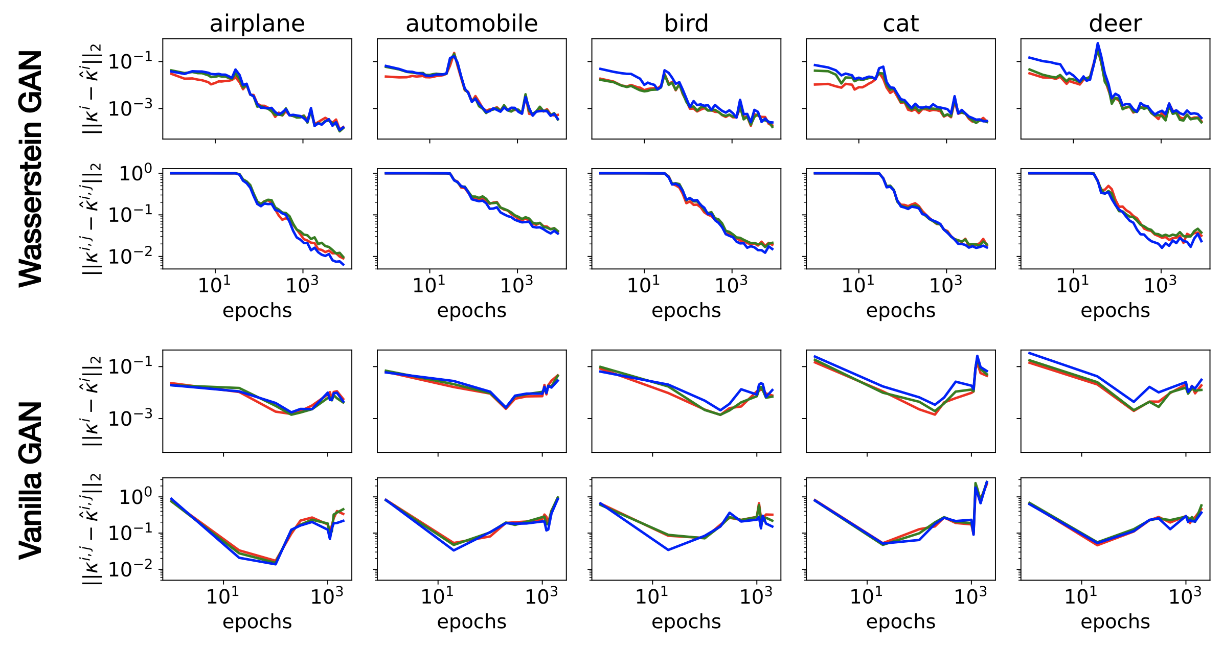
Figure B.2: Evolution of the mean and covariance of GAN-generated images during training. We plot the mean-squared difference between in the mean $\kappa^{i}$ and covariance $\kappa^{i,j}$ between CIFAR10 images and samples from a GAN trained on images from that class, $\hat{\kappa}^{i}$, throughout training of the GAN. The top and bottom two rows show results for the Wasserstein and vanilla GAN, respectively. We only show the first five classes, results for the other five classes were similar. Different colours correspond to the three different colour channels.

B.2 Architectures and training procedures

For our experiments on CIFAR10 (Section 3), we used the following architectures.

Two-layer network

Two fully-connected layers acting on greyscale images; ReLU activation function, 512 neurons on CIFAR10, 2048 hidden neurons on CIFAR100. Parameters: Trained with SGD with learning rate 0.005, weight decay $5e^{-4}$, no momentum, mini-batch size 64.

LeNet

LeNet5 architecture of LeCun et al. (1998) with five layers; the final layer before the linear classifier had 84 neurons for CIFAR10 and 120 neurons for CIFAR100.

DenseNet121, ViT, Resnet18

We used the implementation of these models and the pre-trained weights available in the timm library (Wightman, 2019). For Densenet121 and Resnet18, we made a slight modification to the first convolutional layer, choosing a smaller kernel width, 3 instead of 7, at padding=1, stride=1. We also removed the first pooling layer before the first residual block. The idea behind this change is to avoid the strong downsampling of these architectures in the first layer. The downsampling is fine (or even necessary) for the large images of ImageNet, for which these networks were designed, but it removes too much information from the smaller CIFAR images and thus seriously degrades performance. We did not apply this modification for the pre-trained networks of Section 3.1, since they were pretrained on ImageNet.

We trained all networks except the two-layer network using with SGD with learning rate 0.005, cosine learning rate schedule (Loshchilov & Hutter, 2017), weight decay $5e^{-4}$, momentum 0.9, mini-batch size 128, for 200 epochs. During training, images were randomly cropped with a padding of 4 pixels, and randomly flipped along the horizontal.

Comment on the accuracy improvement of ResNet18 after pre-training

The original ResNet18 architecture achieves $88\%$ test accuracy on CIFAR10 after pre-training on ImageNet (cf. Figure 5A). This performance should not be compared to the $\approx 92\%$ test accuracy of the ResNet18 achieved in our experiments of Section 3, since we modified the first layer of that ResNet to adjust for the image size of CIFAR10 (see above). The performance of the original ResNet18 architecture trained from scratch without this modification when is $85\%$.

Appendix C Experiments on CIFAR100

We repeated the experiment on distributions of increasing complexity on CIFAR100, which has the same image format as CIFAR10, but contains 100 classes with 500 training and 100 test samples each (Krizhevsky et al., 2009). We repeated the experimental protocol of the CIFAR10 experiments from Section 3 with the same architectures; the results are shown in Figure C.1 and discussed in Section 4.

As we discuss in the main text, our computational facilities didn’t allow to train a separate GAN for all 100 clases of CIFAR10. We therefore only repeated the experiments with a Gaussian clone of CIFAR100. While we see that GM/CIFAR100 yields the same test error as CIFAR100/CIFAR100 in the beginning of training for the two-layer network and LeNet, for deeper architectures the discrepancy appears very early during training. We leave it to further work to obtain more accurate approximations of CIFAR100 to verify 1 on this data set, too.

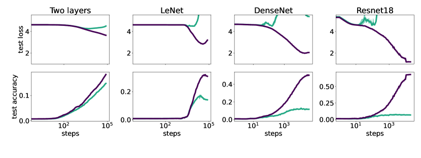
Figure C.1: Test loss and accuracy of neural networks evaluated on CIFAR100 We repeat the experiment of Figure 4 for CIFAR100: we show the test loss and accuracy (top and bottom row, respectively) of various neural networks evaluated on CIFAR100 during training on CIFAR100 and a Gaussian clone of CIFAR100 with 100 Gaussians. We show the mean (solid line) over three runs, starting from the same initial condition each time. The shaded areas indicate minimum and maximum values over the three runs. Full details on the architectures and training recipes are given in Appendix C.

References

- Achille et al. (2019) Achille, A., Rovere, M., and Soatto, S. Critical learning periods in deep networks. In Proc. of ICLR. OpenReview.net, 2019.
- Advani et al. (2020) Advani, M., Saxe, A., and Sompolinsky, H. High-dimensional dynamics of generalization error in neural networks. Neural Networks, 132:428 – 446, 2020.
- Alain & Bengio (2017) Alain, G. and Bengio, Y. Understanding intermediate layers using linear classifier probes. In International Conference on Learning Representations, 2017.
- Amari (1998) Amari, S.-I. Natural gradient works efficiently in learning. Neural computation, 10(2):251–276, 1998.
- Ansuini et al. (2019) Ansuini, A., Laio, A., Macke, J. H., and Zoccolan, D. Intrinsic dimension of data representations in deep neural networks. In Wallach, H. M., Larochelle, H., Beygelzimer, A., d’Alché-Buc, F., Fox, E. B., and Garnett, R. (eds.), Advances in Neural Information Processing Systems 32: Annual Conference on Neural Information Processing Systems 2019, NeurIPS 2019, December 8-14, 2019, Vancouver, BC, Canada, pp. 6109–6119, 2019.
- Arjovsky et al. (2017) Arjovsky, M., Chintala, S., and Bottou, L. Wasserstein generative adversarial networks. In Precup, D. and Teh, Y. W. (eds.), Proc. of ICML, volume 70 of Proceedings of Machine Learning Research, pp. 214–223. PMLR, 2017.
- Arora et al. (2019) Arora, S., Cohen, N., Hu, W., and Luo, Y. Implicit regularization in deep matrix factorization. In Wallach, H. M., Larochelle, H., Beygelzimer, A., d’Alché-Buc, F., Fox, E. B., and Garnett, R. (eds.), Advances in Neural Information Processing Systems 32: Annual Conference on Neural Information Processing Systems 2019, NeurIPS 2019, December 8-14, 2019, Vancouver, BC, Canada, pp. 7411–7422, 2019.
- Arpit et al. (2017) Arpit, D., Jastrzebski, S., Ballas, N., Krueger, D., Bengio, E., Kanwal, M. S., Maharaj, T., Fischer, A., Courville, A. C., Bengio, Y., and Lacoste-Julien, S. A closer look at memorization in deep networks. In Precup, D. and Teh, Y. W. (eds.), Proc. of ICML, volume 70 of Proceedings of Machine Learning Research, pp. 233–242. PMLR, 2017.
- Bach (2017) Bach, F. Breaking the curse of dimensionality with convex neural networks. The Journal of Machine Learning Research, 18(1):629–681, 2017.
- Bau et al. (2017) Bau, D., Zhou, B., Khosla, A., Oliva, A., and Torralba, A. Network dissection: Quantifying interpretability of deep visual representations. In 2017 IEEE Conference on Computer Vision and Pattern Recognition, CVPR 2017, Honolulu, HI, USA, July 21-26, 2017, pp. 3319–3327. IEEE Computer Society, 2017. doi: 10.1109/CVPR.2017.354.
- Bishop (2006) Bishop, C. Pattern recognition and machine learning. Springer, New York, 2006.
- Bordelon et al. (2020) Bordelon, B., Canatar, A., and Pehlevan, C. Spectrum dependent learning curves in kernel regression and wide neural networks. In Proc. of ICML, volume 119 of Proceedings of Machine Learning Research, pp. 1024–1034. PMLR, 2020.
- Bowman & Montúfar (2022) Bowman, B. and Montúfar, G. Implicit bias of MSE gradient optimization in underparameterized neural networks. In Proc. of ICLR. OpenReview.net, 2022.
- Brutzkus et al. (2018) Brutzkus, A., Globerson, A., Malach, E., and Shalev-Shwartz, S. SGD learns over-parameterized networks that provably generalize on linearly separable data. In Proc. of ICLR. OpenReview.net, 2018.
- Chizat et al. (2019) Chizat, L., Oyallon, E., and Bach, F. R. On lazy training in differentiable programming. In Wallach, H. M., Larochelle, H., Beygelzimer, A., d’Alché-Buc, F., Fox, E. B., and Garnett, R. (eds.), Advances in Neural Information Processing Systems 32: Annual Conference on Neural Information Processing Systems 2019, NeurIPS 2019, December 8-14, 2019, Vancouver, BC, Canada, pp. 2933–2943, 2019.
- Cho & Suh (2019) Cho, J. and Suh, C. Wasserstein gan can perform pca. In 2019 57th Annual Allerton Conference on Communication, Control, and Computing (Allerton), pp. 895–901. IEEE, 2019.
- Deng et al. (2009) Deng, J., Dong, W., Socher, R., Li, L., Li, K., and Li, F. Imagenet: A large-scale hierarchical image database. In 2009 IEEE Computer Society Conference on Computer Vision and Pattern Recognition (CVPR 2009), 20-25 June 2009, Miami, Florida, USA, pp. 248–255. IEEE Computer Society, 2009. doi: 10.1109/CVPR.2009.5206848.
- Doimo et al. (2020) Doimo, D., Glielmo, A., Ansuini, A., and Laio, A. Hierarchical nucleation in deep neural networks. In Larochelle, H., Ranzato, M., Hadsell, R., Balcan, M., and Lin, H. (eds.), Advances in Neural Information Processing Systems 33: Annual Conference on Neural Information Processing Systems 2020, NeurIPS 2020, December 6-12, 2020, virtual, 2020.
- Dosovitskiy et al. (2021) Dosovitskiy, A., Beyer, L., Kolesnikov, A., Weissenborn, D., Zhai, X., Unterthiner, T., Dehghani, M., Minderer, M., Heigold, G., Gelly, S., Uszkoreit, J., and Houlsby, N. An image is worth 16x16 words: Transformers for image recognition at scale. In Proc. of ICLR. OpenReview.net, 2021.
- Engel & Van den Broeck (2001) Engel, A. and Van den Broeck, C. Statistical Mechanics of Learning. Cambridge University Press, 2001.
- Farnia et al. (2018) Farnia, F., Zhang, J., and Tse, D. A spectral approach to generalization and optimization in neural networks. In ICLR, 2018.
- Fischer et al. (2022) Fischer, K., René, A., Keup, C., Layer, M., Dahmen, D., and Helias, M. Decomposing neural networks as mappings of correlation functions. Physical Review Research, 4(4):043143, 2022.
- Gerace et al. (2022) Gerace, F., Krzakala, F., Loureiro, B., Stephan, L., and Zdeborová, L. Gaussian universality of linear classifiers with random labels in high-dimension. 2022.
- Ghorbani et al. (2020) Ghorbani, B., Mei, S., Misiakiewicz, T., and Montanari, A. When do neural networks outperform kernel methods? In Larochelle, H., Ranzato, M., Hadsell, R., Balcan, M., and Lin, H. (eds.), Advances in Neural Information Processing Systems 33: Annual Conference on Neural Information Processing Systems 2020, NeurIPS 2020, December 6-12, 2020, virtual, 2020.
- Goldt et al. (2020) Goldt, S., Mézard, M., Krzakala, F., and Zdeborová, L. Modeling the influence of data structure on learning in neural networks: The hidden manifold model. Phys. Rev. X, 10(4):041044, 2020.
- Goldt et al. (2022) Goldt, S., Loureiro, B., Reeves, G., Krzakala, F., Mezard, M., and Zdeborová, L. The gaussian equivalence of generative models for learning with shallow neural networks. In Bruna, J., Hesthaven, J., and Zdeborová, L. (eds.), Proceedings of the 2nd Mathematical and Scientific Machine Learning Conference, volume 145 of Proceedings of Machine Learning Research, pp. 426–471. PMLR, 2022.
- Goodfellow et al. (2014) Goodfellow, I. J., Pouget-Abadie, J., Mirza, M., Xu, B., Warde-Farley, D., Ozair, S., Courville, A. C., and Bengio, Y. Generative adversarial nets. In Ghahramani, Z., Welling, M., Cortes, C., Lawrence, N. D., and Weinberger, K. Q. (eds.), Advances in Neural Information Processing Systems 27: Annual Conference on Neural Information Processing Systems 2014, December 8-13 2014, Montreal, Quebec, Canada, pp. 2672–2680, 2014.
- Gulrajani et al. (2017) Gulrajani, I., Ahmed, F., Arjovsky, M., Dumoulin, V., and Courville, A. C. Improved training of wasserstein gans. In Guyon, I., von Luxburg, U., Bengio, S., Wallach, H. M., Fergus, R., Vishwanathan, S. V. N., and Garnett, R. (eds.), Advances in Neural Information Processing Systems 30: Annual Conference on Neural Information Processing Systems 2017, December 4-9, 2017, Long Beach, CA, USA, pp. 5767–5777, 2017.
- Gunasekar et al. (2017) Gunasekar, S., Woodworth, B. E., Bhojanapalli, S., Neyshabur, B., and Srebro, N. Implicit regularization in matrix factorization. In Guyon, I., von Luxburg, U., Bengio, S., Wallach, H. M., Fergus, R., Vishwanathan, S. V. N., and Garnett, R. (eds.), Advances in Neural Information Processing Systems 30: Annual Conference on Neural Information Processing Systems 2017, December 4-9, 2017, Long Beach, CA, USA, pp. 6151–6159, 2017.
- Gunasekar et al. (2018) Gunasekar, S., Lee, J. D., Soudry, D., and Srebro, N. Implicit bias of gradient descent on linear convolutional networks. In Bengio, S., Wallach, H. M., Larochelle, H., Grauman, K., Cesa-Bianchi, N., and Garnett, R. (eds.), Advances in Neural Information Processing Systems 31: Annual Conference on Neural Information Processing Systems 2018, NeurIPS 2018, December 3-8, 2018, Montréal, Canada, pp. 9482–9491, 2018.
- He et al. (2016) He, K., Zhang, X., Ren, S., and Sun, J. Deep residual learning for image recognition. In 2016 IEEE Conference on Computer Vision and Pattern Recognition, CVPR 2016, Las Vegas, NV, USA, June 27-30, 2016, pp. 770–778. IEEE Computer Society, 2016. doi: 10.1109/CVPR.2016.90.
- Ho et al. (2020) Ho, J., Jain, A., and Abbeel, P. Denoising diffusion probabilistic models. In Larochelle, H., Ranzato, M., Hadsell, R., Balcan, M., and Lin, H. (eds.), Advances in Neural Information Processing Systems 33: Annual Conference on Neural Information Processing Systems 2020, NeurIPS 2020, December 6-12, 2020, virtual, 2020.
- Hu & Lu (2022) Hu, H. and Lu, Y. M. Universality laws for high-dimensional learning with random features. IEEE Transactions on Information Theory, 2022.
- Huang et al. (2017) Huang, G., Liu, Z., van der Maaten, L., and Weinberger, K. Q. Densely connected convolutional networks. In 2017 IEEE Conference on Computer Vision and Pattern Recognition, CVPR 2017, Honolulu, HI, USA, July 21-26, 2017, pp. 2261–2269. IEEE Computer Society, 2017. doi: 10.1109/CVPR.2017.243.
- Ingrosso & Goldt (2022) Ingrosso, A. and Goldt, S. Data-driven emergence of convolutional structure in neural networks. Proceedings of the National Academy of Sciences, 119(40):e2201854119, 2022. doi: 10.1073/pnas.2201854119.
- Ji & Telgarsky (2019) Ji, Z. and Telgarsky, M. The implicit bias of gradient descent on nonseparable data. In Beygelzimer, A. and Hsu, D. (eds.), Conference on Learning Theory, COLT 2019, 25-28 June 2019, Phoenix, AZ, USA, volume 99 of Proceedings of Machine Learning Research, pp. 1772–1798. PMLR, 2019.
- Ji & Telgarsky (2020) Ji, Z. and Telgarsky, M. Directional convergence and alignment in deep learning. In Larochelle, H., Ranzato, M., Hadsell, R., Balcan, M., and Lin, H. (eds.), Advances in Neural Information Processing Systems 33: Annual Conference on Neural Information Processing Systems 2020, NeurIPS 2020, December 6-12, 2020, virtual, 2020.
- Jin & Montúfar (2020) Jin, H. and Montúfar, G. Implicit bias of gradient descent for mean squared error regression with wide neural networks. 2020.
- Kalimeris et al. (2019) Kalimeris, D., Kaplun, G., Nakkiran, P., Edelman, B. L., Yang, T., Barak, B., and Zhang, H. SGD on neural networks learns functions of increasing complexity. In Wallach, H. M., Larochelle, H., Beygelzimer, A., d’Alché-Buc, F., Fox, E. B., and Garnett, R. (eds.), Advances in Neural Information Processing Systems 32: Annual Conference on Neural Information Processing Systems 2019, NeurIPS 2019, December 8-14, 2019, Vancouver, BC, Canada, pp. 3491–3501, 2019.
- Kataoka et al. (2020) Kataoka, H., Okayasu, K., Matsumoto, A., Yamagata, E., Yamada, R., Inoue, N., Nakamura, A., and Satoh, Y. Pre-training without natural images. In Proceedings of the Asian Conference on Computer Vision (ACCV), 2020.
- Kolda & Bader (2009) Kolda, T. G. and Bader, B. W. Tensor decompositions and applications. SIAM review, 51(3):455–500, 2009.
- Kolesnikov et al. (2020) Kolesnikov, A., Beyer, L., Zhai, X., Puigcerver, J., Yung, J., Gelly, S., and Houlsby, N. Big transfer (bit): General visual representation learning. In European conference on computer vision, pp. 491–507. Springer, 2020.
- Krishna et al. (2021) Krishna, K., Bigham, J., and Lipton, Z. C. Does pretraining for summarization require knowledge transfer? In Findings of the Association for Computational Linguistics: EMNLP 2021, pp. 3178–3189, Punta Cana, Dominican Republic, 2021. Association for Computational Linguistics. doi: 10.18653/v1/2021.findings-emnlp.273.
- Krizhevsky et al. (2009) Krizhevsky, A., Hinton, G., et al. Learning multiple layers of features from tiny images. https://www.cs.toronto.edu/ kriz/learning-features-2009-TR.pdf, 2009.
- Krogh & Hertz (1992) Krogh, A. and Hertz, J. A. Generalization in a linear perceptron in the presence of noise. Journal of Physics A: Mathematical and General, 25(5):1135, 1992.
- Le Cun et al. (1991) Le Cun, Y., Kanter, I., and Solla, S. A. Eigenvalues of covariance matrices: Application to neural-network learning. Physical Review Letters, 66(18):2396, 1991.
- LeCun et al. (1998) LeCun, Y., Bottou, L., Bengio, Y., and Haffner, P. Gradient-based learning applied to document recognition. Proceedings of the IEEE, 86(11):2278–2324, 1998. doi: 10.1109/5.726791.
- Li et al. (2018) Li, Y., Ma, T., and Zhang, H. Algorithmic regularization in over-parameterized matrix sensing and neural networks with quadratic activations. In Bubeck, S., Perchet, V., and Rigollet, P. (eds.), Conference On Learning Theory, COLT 2018, Stockholm, Sweden, 6-9 July 2018, volume 75 of Proceedings of Machine Learning Research, pp. 2–47. PMLR, 2018.
- Liao & Couillet (2018) Liao, Z. and Couillet, R. On the spectrum of random features maps of high dimensional data. In Dy, J. G. and Krause, A. (eds.), Proc. of ICML, volume 80 of Proceedings of Machine Learning Research, pp. 3069–3077. PMLR, 2018.
- Liu et al. (2020) Liu, S., Papailiopoulos, D. S., and Achlioptas, D. Bad global minima exist and SGD can reach them. In Larochelle, H., Ranzato, M., Hadsell, R., Balcan, M., and Lin, H. (eds.), Advances in Neural Information Processing Systems 33: Annual Conference on Neural Information Processing Systems 2020, NeurIPS 2020, December 6-12, 2020, virtual, 2020.
- Loshchilov & Hutter (2017) Loshchilov, I. and Hutter, F. SGDR: stochastic gradient descent with warm restarts. In Proc. of ICLR. OpenReview.net, 2017.
- Loureiro et al. (2021a) Loureiro, B., Gerbelot, C., Cui, H., Goldt, S., Krzakala, F., Mézard, M., and Zdeborová, L. Learning curves of generic features maps for realistic datasets with a teacher-student model. In Ranzato, M., Beygelzimer, A., Dauphin, Y. N., Liang, P., and Vaughan, J. W. (eds.), Advances in Neural Information Processing Systems 34: Annual Conference on Neural Information Processing Systems 2021, NeurIPS 2021, December 6-14, 2021, virtual, pp. 18137–18151, 2021a.
- Loureiro et al. (2021b) Loureiro, B., Sicuro, G., Gerbelot, C., Pacco, A., Krzakala, F., and Zdeborová, L. Learning gaussian mixtures with generalized linear models: Precise asymptotics in high-dimensions. In Ranzato, M., Beygelzimer, A., Dauphin, Y. N., Liang, P., and Vaughan, J. W. (eds.), Advances in Neural Information Processing Systems 34: Annual Conference on Neural Information Processing Systems 2021, NeurIPS 2021, December 6-14, 2021, virtual, pp. 10144–10157, 2021b.
- Lukacs (1970) Lukacs, E. Characteristic Functions. Griffin, London, second edition, 1970.
- Lyu & Li (2020) Lyu, K. and Li, J. Gradient descent maximizes the margin of homogeneous neural networks. In Proc. of ICLR. OpenReview.net, 2020.
- Maennel et al. (2020) Maennel, H., Alabdulmohsin, I. M., Tolstikhin, I. O., Baldock, R. J. N., Bousquet, O., Gelly, S., and Keysers, D. What do neural networks learn when trained with random labels? In Larochelle, H., Ranzato, M., Hadsell, R., Balcan, M., and Lin, H. (eds.), Advances in Neural Information Processing Systems 33: Annual Conference on Neural Information Processing Systems 2020, NeurIPS 2020, December 6-12, 2020, virtual, 2020.
- Mangalam & Prabhu (2019) Mangalam, K. and Prabhu, V. U. Do deep neural networks learn shallow learnable examples first? In ICML 2019 Workshop on Identifying and Understanding Deep Learning Phenomena, 2019.
- McCullagh (2018) McCullagh, P. Tensor methods in statistics. Chapman and Hall/CRC, 2018.
- Mei & Montanari (2021) Mei, S. and Montanari, A. The generalization error of random features regression: Precise asymptotics and the double descent curve. Communications on Pure and Applied Mathematics, 2021. doi: https://doi.org/10.1002/cpa.22008.
- Mei et al. (2018) Mei, S., Montanari, A., and Nguyen, P. A mean field view of the landscape of two-layer neural networks. Proceedings of the National Academy of Sciences, 115(33):E7665–E7671, 2018.
- Mignacco et al. (2020a) Mignacco, F., Krzakala, F., Lu, Y., Urbani, P., and Zdeborová, L. The role of regularization in classification of high-dimensional noisy gaussian mixture. In Proc. of ICML, volume 119 of Proceedings of Machine Learning Research, pp. 6874–6883. PMLR, 2020a.
- Mignacco et al. (2020b) Mignacco, F., Krzakala, F., Urbani, P., and Zdeborová, L. Dynamical mean-field theory for stochastic gradient descent in gaussian mixture classification. In Larochelle, H., Ranzato, M., Hadsell, R., Balcan, M., and Lin, H. (eds.), Advances in Neural Information Processing Systems 33: Annual Conference on Neural Information Processing Systems 2020, NeurIPS 2020, December 6-12, 2020, virtual, 2020b.
- Mossel (2016) Mossel, E. Deep learning and hierarchical generative models. 2016.
- Nakkiran & Bansal (2020) Nakkiran, P. and Bansal, Y. Distributional generalization: A new kind of generalization. 2020.
- Nakkiran et al. (2021) Nakkiran, P., Neyshabur, B., and Sedghi, H. The bootstrap framework: Generalization through the lens of online optimization. In International Conference on Learning Representations, 2021.
- Neyshabur et al. (2015) Neyshabur, B., Tomioka, R., and Srebro, N. In search of the real inductive bias: On the role of implicit regularization in deep learning. In ICLR, 2015.
- Paszke et al. (2019) Paszke, A., Gross, S., Massa, F., Lerer, A., Bradbury, J., Chanan, G., Killeen, T., Lin, Z., Gimelshein, N., Antiga, L., Desmaison, A., Köpf, A., Yang, E., DeVito, Z., Raison, M., Tejani, A., Chilamkurthy, S., Steiner, B., Fang, L., Bai, J., and Chintala, S. Pytorch: An imperative style, high-performance deep learning library. In Wallach, H. M., Larochelle, H., Beygelzimer, A., d’Alché-Buc, F., Fox, E. B., and Garnett, R. (eds.), Advances in Neural Information Processing Systems 32: Annual Conference on Neural Information Processing Systems 2019, NeurIPS 2019, December 8-14, 2019, Vancouver, BC, Canada, pp. 8024–8035, 2019.
- Pérez et al. (2019) Pérez, G. V., Camargo, C. Q., and Louis, A. A. Deep learning generalizes because the parameter-function map is biased towards simple functions. In Proc. of ICLR. OpenReview.net, 2019.
- Pope et al. (2021) Pope, P., Zhu, C., Abdelkader, A., Goldblum, M., and Goldstein, T. The intrinsic dimension of images and its impact on learning. In Proc. of ICLR. OpenReview.net, 2021.
- Radford et al. (2016) Radford, A., Metz, L., and Chintala, S. Unsupervised representation learning with deep convolutional generative adversarial networks. In Bengio, Y. and LeCun, Y. (eds.), Proc. of ICLR, 2016.
- Raghu et al. (2017) Raghu, M., Gilmer, J., Yosinski, J., and Sohl-Dickstein, J. SVCCA: singular vector canonical correlation analysis for deep learning dynamics and interpretability. In Guyon, I., von Luxburg, U., Bengio, S., Wallach, H. M., Fergus, R., Vishwanathan, S. V. N., and Garnett, R. (eds.), Advances in Neural Information Processing Systems 30: Annual Conference on Neural Information Processing Systems 2017, December 4-9, 2017, Long Beach, CA, USA, pp. 6076–6085, 2017.
- Rahaman et al. (2019) Rahaman, N., Baratin, A., Arpit, D., Draxler, F., Lin, M., Hamprecht, F. A., Bengio, Y., and Courville, A. C. On the spectral bias of neural networks. In Chaudhuri, K. and Salakhutdinov, R. (eds.), Proc. of ICML, volume 97 of Proceedings of Machine Learning Research, pp. 5301–5310. PMLR, 2019.
- Refinetti & Goldt (2022) Refinetti, M. and Goldt, S. The dynamics of representation learning in shallow, non-linear autoencoders. In Chaudhuri, K., Jegelka, S., Song, L., Szepesvári, C., Niu, G., and Sabato, S. (eds.), International Conference on Machine Learning, ICML 2022, 17-23 July 2022, Baltimore, Maryland, USA, volume 162 of Proceedings of Machine Learning Research, pp. 18499–18519. PMLR, 2022.
- Refinetti et al. (2021) Refinetti, M., Goldt, S., Krzakala, F., and Zdeborová, L. Classifying high-dimensional gaussian mixtures: Where kernel methods fail and neural networks succeed. In Meila, M. and Zhang, T. (eds.), Proc. of ICML, volume 139 of Proceedings of Machine Learning Research, pp. 8936–8947. PMLR, 2021.
- Saad & Solla (1995) Saad, D. and Solla, S. Exact Solution for On-Line Learning in Multilayer Neural Networks. Phys. Rev. Lett., 74(21):4337–4340, 1995.
- Saxe et al. (2019) Saxe, A., McClelland, J., and Ganguli, S. A mathematical theory of semantic development in deep neural networks. Proceedings of the National Academy of Sciences, 116(23):11537–11546, 2019.
- Saxe et al. (2014) Saxe, A. M., McClelland, J. L., and Ganguli, S. Exact solutions to the nonlinear dynamics of learning in deep linear neural networks. In Bengio, Y. and LeCun, Y. (eds.), Proc. of ICLR, 2014.
- Schwarze & Hertz (1992) Schwarze, H. and Hertz, J. Generalization in a large committee machine. EPL (Europhysics Letters), 20(4):375, 1992.
- Seddik et al. (2019) Seddik, M. E. A., Tamaazousti, M., and Couillet, R. Kernel random matrices of large concentrated data: the example of gan-generated images. In IEEE International Conference on Acoustics, Speech and Signal Processing, ICASSP 2019, Brighton, United Kingdom, May 12-17, 2019, pp. 7480–7484. IEEE, 2019. doi: 10.1109/ICASSP.2019.8683333.
- Soudry et al. (2018) Soudry, D., Hoffer, E., Nacson, M. S., and Srebro, N. The implicit bias of gradient descent on separable data. In Proc. of ICLR. OpenReview.net, 2018.
- Spigler et al. (2020) Spigler, S., Geiger, M., and Wyart, M. Asymptotic learning curves of kernel methods: empirical data versus teacher–student paradigm. Journal of Statistical Mechanics: Theory and Experiment, 2020(12):124001, 2020.
- van Amersfoort (2021) van Amersfoort, J. Minimal CIFAR10. https://github.com/y0ast/pytorch-snippets/tree/main/minimal_cifar, 2021.
- Vardi (2022) Vardi, G. On the implicit bias in deep-learning algorithms. ArXiv preprint, abs/2208.12591, 2022.
- Vaswani et al. (2017) Vaswani, A., Shazeer, N., Parmar, N., Uszkoreit, J., Jones, L., Gomez, A. N., Kaiser, L., and Polosukhin, I. Attention is all you need. In Guyon, I., von Luxburg, U., Bengio, S., Wallach, H. M., Fergus, R., Vishwanathan, S. V. N., and Garnett, R. (eds.), Advances in Neural Information Processing Systems 30: Annual Conference on Neural Information Processing Systems 2017, December 4-9, 2017, Long Beach, CA, USA, pp. 5998–6008, 2017.
- Wightman (2019) Wightman, R. Pytorch image models. https://github.com/rwightman/pytorch-image-models, 2019.
- Xu (2018) Xu, Z. J. Understanding training and generalization in deep learning by fourier analysis. ArXiv preprint, abs/1808.04295, 2018.
- Yang et al. (2022) Yang, G., Ajay, A., and Agrawal, P. Overcoming the spectral bias of neural value approximation. In Proc. of ICLR. OpenReview.net, 2022.