Adaptive Constraint Partition based Optimization Framework for Large-scale Integer Linear Programming(Student Abstract)

Abstract

Integer programming problems (IPs) are challenging to be solved efficiently due to the NP-hardness, especially for large-scale IPs. To solve this type of IPs, Large neighborhood search (LNS) uses an initial feasible solution and iteratively improves it by searching a large neighborhood around the current solution. However, LNS easily steps into local optima and ignores the correlation between variables to be optimized, leading to compromised performance. This paper presents a general adaptive constraint partition-based optimization framework (ACP) for large-scale IPs that can efficiently use any existing optimization solver as a subroutine. Specifically, ACP first randomly partitions the constraints into blocks, where the number of blocks is adaptively adjusted to avoid local optima. Then, ACP uses a subroutine solver to optimize the decision variables in a randomly selected block of constraints to enhance the variable correlation. ACP is compared with LNS framework with different subroutine solvers on four IPs and a real-world IP. The experimental results demonstrate that in specified wall-clock time ACP shows better performance than SCIP and Gurobi.

Introduction

Integer programming problems (IPs) are usually NP-hard, and their algorithm design is challenging and research-worthy. Even with advances, the performance of traditional tree algorithms for IPs, such as branch-and-bound (Zarpellon et al. 2021) and branch-and-cut (Huang et al. 2022), decrease severely in high-dimensional search spaces. Therefore, Large neighborhood search (LNS) (Shaw 1998; Pisinger and Ropke 2010; Song and ohters 2020), defining neighborhoods and optimizing blocks that contain a subset of decision variables, has been widely used and achieved good results for many real-world large-scale IPs(Sonnerat et al. 2021; Li et al. 2022). However, for IPs with millions of decision variables, the traditional LNS frameworks ignore the correlation between variables and easily step into local optima due to the fixed number of blocks. This paper proposes ACP to address the above two issues. The key idea of ACP is that it adaptively updates the number of blocks to avoid local optima, and uses a two-step variable selection method to enhance the correlation between variables to be optimized. Results on four large-scale IPs and a real-world IP verify the effectiveness of ACP.

Method

As shown in Algorithm 1, ACP starts with an initial feasible solution that is artificially constructed, and iteratively improves the current solution. Then, constraints are randomly partitioned into disjoint blocks (Step 2). Each iteration only considers one block and the variables in this block are optimized, while other variables are fixed with the value of the current optimal feasible solution (Step 3-5). The number of blocks is updated according to the objective value improvement of recent two iterations with a pre-set threshold (Step 6-7). Based on ACP, the ACP2 framework is derived that uses the subroutine solver instead of artificially constructing to generate an initial feasible solution.

Algorithm 1 The framework of ACP

Input: An IP $P$ with constraints $C$ and variables $X$, an initial feasible solution $S_{X}$, a subroutine solver $F$
  Output: A solution $S_{X}$

1:while Specified wall-clock time not met do

2:     $C=C_{1}\cup C_{2}\cup\dots\cup C_{k-1}\cup C_{k}$ $\triangleright$ Constraint Partition

3:     $X_{sub}\leftarrow$ variables selected in a random block $C_{i}$

4:     $X_{opt}\leftarrow S_{X}$

5:     $S_{X}\leftarrow\text{FIX\_OPTIMIZE(}P,S_{X},X_{sub},F\text{)}$$\triangleright$ Optimization

6:     if $f(S_{X})-f(X_{opt})<\epsilon f(X_{opt})$ then $\triangleright$ Block Update

7:         $k\leftarrow k-1$

8:     end if

9:end while

10:return $S_{X}$

Constraint Partition. For an IP $P$ with the decision variable set $X$ and the constraint set $C$, ACP randomly divides $C$ into $k$ disjoint blocks $C_{1},C_{2},\dots,C_{k}$ where $C=C_{1}\cup C_{2}\cup\dots\cup C_{k}$ and $C_{i}\cap C_{j}=\emptyset$, $i\neq j$, $i,j\in[1,\dots,k]$. $k$ is a hyperparameter that is different for different IPs.

Optimization. At each iteration, one block $C_{i}$($i\in[1,\dots,k]$) is randomly selected, and $C_{i}$ differs at different iterations. Given a feasible solution $S_{x}$ of the current IP $P$, all decision variables $X_{sub}$ in the randomly selected subset $C_{i}$ are treated as the local neighborhood of the search. Then in function FIX_OPTIMIZE, a subroutine solver $F$ (SCIP, Gurobi) is used to search the optimal solution of a sub-IP with decision variable set $X_{sub}$. All integer variables in $X\setminus X_{sub}$ are fixed with the value of the current optimal feasible solution $X_{opt}$. The new solution $S_{X}$ is obtained by recombining $X_{sub}$ and $X\setminus X_{sub}$.

Block update. To avoid getting stuck in local optima, ACP updates the number of blocks $k$ with an optimization threshold of objective value improvement $\epsilon$. If the improvement rate $f(S_{X})-f(X_{opt})$ of the objective function $f(S_{X})$ after one iteration is less than $\epsilon$, the current solution is likely to be a local optimum. In this case, ACP reduces the number of blocks $k$ to expand the neighborhood to jump out of the local optimum. Additional details such as the initial block number $k$ and optimization threshold $\epsilon$ are given in the appendix.

Experiments

Experimental Settings. With different subroutine solvers, we compare ACP with LNS framework (Song and ohters 2020) and the original subroutine solver on maximum independent set (IS), minimum vertex cover (MVC), maximum cut (MAXCUT), minimum set covering(SC) and one real-world large-scale IP in the internet domain. For IS, MVC and MAXCUT, we use random graphs of 1,000,000 points and 3,000,000 edges. For SC, we use random problem of 1,000,000 items and 1,000,000 sets. For the real-world large-scale IP, it has more than 800,000 decision variables and 50,000 constraints. All experiments are repeated 5 times and the average of the metric is recorded.

Results and Analysis. Table 1 shows the results of all the related methods on five IPs, and the best results are in bold fonts. It can be seen that ACP reliably offers remarkable improvements over LNS framework with different subroutine solvers and the original subroutine solver. Compared with SCIP, ACP obviously achieves much better performance, especially for MAXCUT, SC and the real-world IP. Although the improvement compared with Gurobi is lower than that of SCIP, ACP still outperforms Gurobi on all the five IPs. We also find that with block partition and adaptive update of block number, ACP improves the performance of LNS.

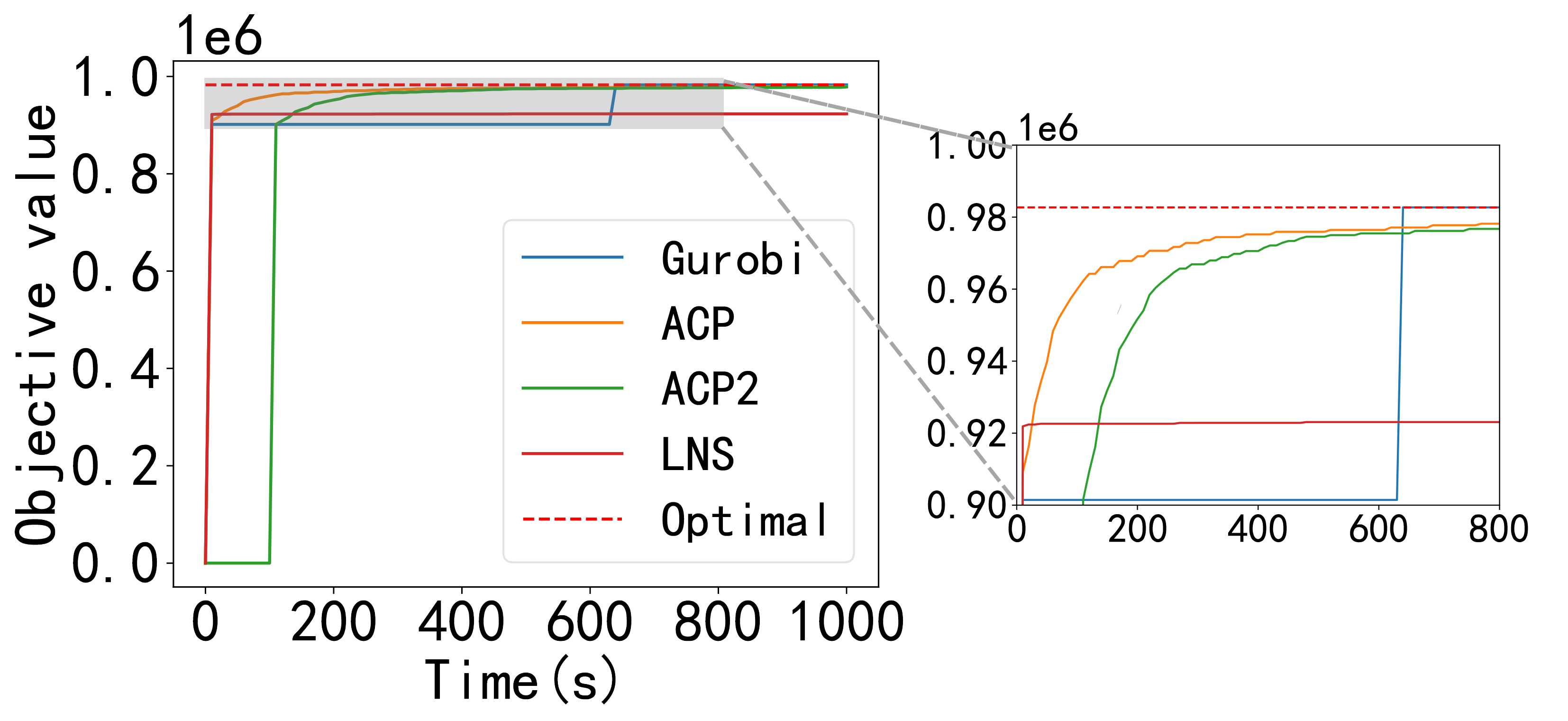
Figure 1: The objective value variation for real-world IP.

For clearer comparison, we further show the objective value variation with running time for the real-world large-scale IP in Figure 1. It can be found that ACP exhibits noteworthy advantages within limited wall-clock time, which can find the approximate optimal solution faster than other methods, even for the fastest commercial solver Gurobi. Due to the length limitation, we show other comparison results of all the related methods on small, medium and large-scale IPs in the appendix. The results also demonstrate the obvious advantages of ACP over other baseline methods.

Problem	SCIP based	Objective value	Gurobi based	Objective value
IS (Maximize)	SCIP	7866.55 $\pm$ 55.47	Gurobi	215365.65 $\pm$ 113.5
	LNS	194733.92 $\pm$ 79.17	LNS	220368.34 $\pm$ 557.89
	ACP	207901.54 $\pm$ 1531.18	ACP	227559.62 $\pm$ 57.26
	ACP2	196742.1 $\pm$ 116.6	ACP2	227636.51 $\pm$ 432.18
MVC (Minimize)	SCIP	490857.44 $\pm$ 164.24	Gurobi	283170.59 $\pm$ 317.06
	LNS	304860.39 $\pm$ 313.2	LNS	277870.09 $\pm$ 300.8
	ACP	291226.0 $\pm$ 1189.94	ACP	271163.92 $\pm$ 337.0
	ACP2	301836.42 $\pm$ 70.59	ACP2	271087.22 $\pm$ 295.85
MAXCUT (Maximize)	SCIP	9.02 $\pm$ 1.24	Gurobi	971138.1 $\pm$ 308.18
	LNS	553840.66 $\pm$ 45172.75	LNS	910662.36 $\pm$ 516.31
	ACP	829597.17 $\pm$ 46331.3	ACP	1050400.97 $\pm$ 106.3
	ACP2	747434.19 $\pm$ 48697.78	ACP2	1053583.50 $\pm$ 473.43
SC (Minimize)	SCIP	919264.06 $\pm$ 607.75	Gurobi	320034.15 $\pm$ 208.69
	LNS	584210.54 $\pm$ 158940.18	LNS	224435.73 $\pm$ 1253.96
	ACP	392082.53 $\pm$ 10206.15	ACP	208062.73 $\pm$ 5582.97
	ACP2	432368.51 $\pm$ 615.53	ACP2	201034.73 $\pm$ 196.14
Read-world IP (Maximize)	SCIP	0.0 $\pm$ 0.0	Gurobi	903119.36 $\pm$ 1588.62
	LNS	904387.43 $\pm$ 1560.34	LNS	924886.13 $\pm$ 1670.82
	ACP	909113.41 $\pm$ 2030.01	ACP	948461.41 $\pm$ 4385.63
	ACP2	907155.48 $\pm$ 2199.08	ACP2	942235.76 $\pm$ 1861.36

Table 1: Comparison results for ACP and LNS with different subroutine solvers on different benchmark IPs.

Conclusion

This paper presents ACP for large-scale IPs that can efficiently use any existing optimization solver as a subroutine. The results and analysis show that the ACP framework is obviously superior to the mainstream method in specified wall-clock time. In the future, we will study the combination of LNS and graph neural networks for large-scale IPs.

-Appendix-

Appendix A Experimental Settings

This section shows the experimental settings used in our paper, including the description of all the five IP benchmark problems and implementation details.

Problem Description

To study the performance of ACP, we use four classical integer programming problems (IPs), including maximum independent set (IS), minimum vertex cover (MVC), maximum cut (MAXCUT), minimum set covering (SC), and a real-world problem represented as large-scale IP in this paper. Each of the five IPs contains three kinds of scales, small, medium and large, which include ten thousands of, hundred thousands of and millions of decision variables, respectively. The details of all the IP benchmarks are shown in Table 1. The specified time in Table 1 are the total pre-specified running times for each method on each IP, i.e., the wall-clock time in Algorithm 1.

Scale	Problem	Description	Specified time
Small	IS	10,000 nodes and 30,000 edges	10s
	MVC	10,000 nodes and 30,000 edges	10s
	MAXCUT	10,000 nodes and 30,000 edges	10s
	SC	20,000 items and 20,000 set where each item appears in 4 sets	20s
	Real-world IP	10,000 decision variables	10s
Medium	IS	100,000 nodes and 300,000 edges	100s
	MVC	100,000 nodes and 300,000 edges	100s
	MAXCUT	100,000 nodes and 300,000 edges	180s
	SC	200,000 items and 200,000 set where each item appears in 4 sets	100s
	Real-world IP	100,000 decision variables	50s
Large	IS	1000,000 nodes and 3000,000 edges	1500s
	MVC	1000,000 nodes and 3000,000 edges	1500s
	MAXCUT	1000,000 nodes and 3000,000 edges	1800s
	SC	200,000 items and 200,000 set where each item appears in 4 sets	500s
	Real-world IP	1000,000 decision variables	100s

Table 1: Details of five IP benchmarks.

Implementation details

For a fair comparison, all the related methods are run 5 times with 5 different random seeds on each IP on the same device, Intel Core i9-10900K processor with 10 cores, 2 NVIDIA GeForce RTX 3090 GPU card with 24GB GPU memory. The mean of the results is recorded. For different scales of IP benchmarks, we use different initial numbers of blocks $k$. Table 2 gives all the $k$ cases for IS, MVC, MAXCUT, SC and real-world IP. The $\epsilon$ used to determine the objective value improvement is set to different values for different scales of IPs, which is shown in Table 3.

In the code implementation, to adjust the frequency of dynamic block number changes, we set $t$, which means that when the improvement rates of consecutive $t$ iterations are all less than the threshold $\epsilon$, ACP will reduce the number of blocks $k$ to expand the neighborhood to jump out of the local optimum, as shown in Table 4. To adapt to different problem sizes, we also set $p$, which means the proportion of the maximum running time of each iteration to the total time, as shown in Table 5.

Scale	Problem	Initial block number $k$
		SCIP			Gurobi
		LNS	ACP	ACP2	LNS	ACP	ACP2
Small	IS	2	6	4	2	4	4
	MVC	3	5	4	2	4	4
	MAXCUT	2	3	2	2	3	3
	SC	4	10	10	3	7	8
	Real-world IP	5	10	10	2	3	3
Medium	IS	6	8	8	3	6	6
	MVC	6	8	8	3	6	6
	MAXCUT	4	6	6	4	5	4
	SC	6	12	12	3	5	6
	Real-world IP	6	10	10	3	4	4
Large	IS	8	10	10	6	6	6
	MVC	8	10	10	3	8	8
	MAXCUT	15	15	15	6	10	5
	SC	20	25	25	4	5	5
	Real-world IP	6	50	50	3	7	6

Table 2: The initial block number $k$ of all IPs with small, medium and large scales.

Scale	Problem	Optimization threshold $\epsilon$
		SCIP		Gurobi
		ACP	ACP2	ACP	ACP2
Small	IS	0.002	0.01	0.01	0.01
	MVC	0.002	0.01	0.01	0.01
	MAXCUT	0.1	0.01	0.01	0.01
	SC	0.002	0.01	0.01	0.01
	Real-world IP	0.001	0.05	0.001	0.001
Medium	IS	0.1	0.01	0.01	0.01
	MVC	0.002	0.01	0.01	0.01
	MAXCUT	0.1	0.01	0.005	0.005
	SC	0.002	0.01	0.01	0.01
	Real-world IP	0.02	0.05	0.01	0.0007
Large	IS	0.1	0.01	0.01	0.01
	MVC	0.002	0.01	0.01	0.01
	MAXCUT	0.1	0.01	0.1	0.005
	SC	0.002	0.01	0.01	0.01
	Real-world IP	0.0007	0.0007	0.01	0.0007

Table 3: The optimization threshold $\epsilon$ of all IPs with small, medium and large scales.

Scale	Problem	Maximum iterations $t$
		SCIP		Gurobi
		ACP	ACP2	ACP	ACP2
Small	IS	3	3	3	3
	MVC	3	3	3	3
	MAXCUT	3	3	3	3
	SC	3	3	3	3
	Real-world IP	3	2	3	3
Medium	IS	3	3	3	3
	MVC	3	3	3	3
	MAXCUT	3	3	3	2
	SC	3	3	3	3
	Real-world IP	2	3	3	3
Large	IS	3	3	3	3
	MVC	3	3	3	3
	MAXCUT	3	3	2	2
	SC	3	3	3	3
	Real-world IP	5	5	3	3

Table 4: The maximum consecutive iterations that are all less than the threshold.

Scale	Problem	Maximum proportion $p$
		SCIP			Gurobi
		LNS	ACP	ACP2	LNS	ACP	ACP2
Small	IS	0.1	0.1	0.2	0.1	0.1	0.2
	MVC	0.1	0.1	0.2	0.1	0.1	0.2
	MAXCUT	0.3	0.2	0.3	0.1	0.1	0.2
	SC	0.2	0.2	0.2	0.1	0.1	0.2
	Real-world IP	0.2	0.25	0.3	0.2	0.3	0.1
Medium	IS	0.1	0.1	0.2	0.1	0.1	0.2
	MVC	0.1	0.1	0.2	0.1	0.1	0.2
	MAXCUT	0.1	0.1	0.1	0.1	0.1	0.1
	SC	0.2	0.2	0.2	0.1	0.1	0.2
	Real-world IP	0.2	0.2	0.2	0.2	0.2	0.1
Large	IS	0.1	0.1	0.1	0.2	0.1	0.2
	MVC	0.1	0.1	0.1	0.1	0.1	0.2
	MAXCUT	0.1	0.1	0.1	0.1	0.3	0.2
	SC	0.2	0.2	0.2	0.3	0.3	0.2
	Real-world IP	0.1	0.1	0.1	0.2	0.2	0.1

Table 5: The proportion of the maximum running time of each iteration to the total time.

Appendix B Results on Different Scales of IPs

This section shows additional results of all the related methods on five IP benchmarks with small-scale, medium-scale and large-scale, which are shown in Table 6-8, respectively. The best results are in marked bold fonts.

Specifically, compared with SCIP and Gurobi, ACP framework can explore more solution spaces due to the idea of constraint partition. ACP gets better optimization results on all IPs in specified wall-clock time. Compared with the LNS framework, except for the five IPs of MAXCUT, due to the weak correlation between decision variables, the improvement of ACP compared with LNS is not as huge as compared with SCIP and Gurobi. However, in the MAXCUT problem, due to the existence of a large number of related decision variables and a large number of local optima, the optimization result of LNS is worse than Gurobi. Because ACP uses a two-step variable selection method to improve the correlation between variables to be optimized, and adaptively updates the block number to help jump out of the local optimum, the improvement is obvious compared with LNS on MAXCUT.

Performances on Small-scale IPs

Problem	SCIP based	Objective value	Gurobi based	Objective value
IS (Maximize)	SCIP	1882.61 $\pm$ 23.74	Gurobi	2184.64 $\pm$ 14.21
	LNS	2269.42 $\pm$ 12.02	LNS	2259.93 $\pm$ 7.67
	ACP	2297.58 $\pm$ 13.53	ACP	2291.69 $\pm$ 11.64
	ACP2	2224.61 $\pm$ 166.78	ACP2	2293.66 $\pm$ 10.82
MVC (Minimize)	SCIP	3120.28 $\pm$ 38.69	Gurobi	2791.24 $\pm$ 20.13
	LNS	2821.83 $\pm$ 34.87	LNS	2718.5 $\pm$ 15.9
	ACP	2711.23 $\pm$ 28.55	ACP	2686.44 $\pm$ 11.89
	ACP2	2792.07 $\pm$ 150.51	ACP2	2682.87 $\pm$ 12.5
MAXCUT (Maximize)	SCIP	10827.41 $\pm$ 28.34	Gurobi	10686.93 $\pm$ 53.98
	LNS	10453.03 $\pm$ 38.3	LNS	10616.6 $\pm$ 57.51
	ACP	10503.11 $\pm$ 52.69	ACP	11103.77 $\pm$ 99.91
	ACP2	10827.41 $\pm$ 28.34	ACP2	10995.1 $\pm$ 61.76
SC (Minimize)	SCIP	2507.64 $\pm$ 34.34	Gurobi	1800.23 $\pm$ 14.2
	LNS	1815.14 $\pm$ 26.81	LNS	1693.23 $\pm$ 8.7
	ACP	1656.86 $\pm$ 19.99	ACP	1599.98 $\pm$ 8.85
	ACP2	1665.73 $\pm$ 23.19	ACP2	1604.34 $\pm$ 5.98
Read-world IP (Maximize)	SCIP	18347.46 $\pm$ 22470.99	Gurobi	47378.52 $\pm$ 441.98
	LNS	45694.59 $\pm$ 1098.18	LNS	46375.27 $\pm$ 281.97
	ACP	46163.46 $\pm$ 1205.19	ACP	47352.8 $\pm$ 427.65
	ACP2	45747.41 $\pm$ 1096.76	ACP2	47379.18 $\pm$ 441.2

Table 6: Comparison results for ACP and LNS with different subroutine solvers on different benchmark IPs with small-scale.

Performances on Medium-scale IPs

Problem	SCIP based	Objective value	Gurobi based	Objective value
IS (Maximize)	SCIP	18558.83 $\pm$ 53.08	Gurobi	21633.13 $\pm$ 86.11
	LNS	19715.85 $\pm$ 32.75	LNS	21546.55 $\pm$ 345.81
	ACP	21473.28 $\pm$ 272.57	ACP	22450.62 $\pm$ 383.8
	ACP2	21838.83 $\pm$ 38.04	ACP2	22282.99 $\pm$ 629.87
MVC (Minimize)	SCIP	31341.52 $\pm$ 80.79	Gurobi	28198.25 $\pm$ 32.95
	LNS	30046.58 $\pm$ 146.88	LNS	28054.93 $\pm$ 32.82
	ACP	28267.97 $\pm$ 254.05	ACP	26975.96 $\pm$ 24.43
	ACP2	27926.29 $\pm$ 140.61	ACP2	26981.82 $\pm$ 32.18
MAXCUT (Maximize)	SCIP	0.99 $\pm$ 0.49	Gurobi	100211.7 $\pm$ 3103.54
	LNS	94106.85 $\pm$ 615.97	LNS	95967.95 $\pm$ 1469.23
	ACP	105299.09 $\pm$ 1481.79	ACP	107857.56 $\pm$ 1501.38
	ACP2	100770.17 $\pm$ 2092.36	ACP2	108244.69 $\pm$ 1374.97
SC (Minimize)	SCIP	25166.46 $\pm$ 37.69	Gurobi	17983.52 $\pm$ 40.89
	LNS	24337.91 $\pm$ 265.94	LNS	17910.68 $\pm$ 67.92
	ACP	20950.17 $\pm$ 526.61	ACP	17243.17 $\pm$ 1290.13
	ACP2	22445.23 $\pm$ 1024.17	ACP2	16388.32 $\pm$ 160.84
Read-world IP (Maximize)	SCIP	0.0 $\pm$ 0.0	Gurobi	454388.77 $\pm$ 2536.46
	LNS	454947.14 $\pm$ 2676.46	LNS	465150.57 $\pm$ 2475.65
	ACP	455054.64 $\pm$ 2746.93	ACP	477051.41 $\pm$ 2613.14
	ACP2	454856.64 $\pm$ 2702.49	ACP2	472472.17 $\pm$ 2030.22

Table 7: Comparison results for ACP and LNS with different subroutine solvers on different benchmark IPs with medium-scale.

Performances on Large-scale IPs

Problem	SCIP based	Objective value	Gurobi based	Objective value
IS (Maximize)	SCIP	7866.55 $\pm$ 55.47	Gurobi	215365.65 $\pm$ 113.5
	LNS	194733.92 $\pm$ 79.17	LNS	220368.34 $\pm$ 557.89
	ACP	207901.54 $\pm$ 1531.18	ACP	227559.62 $\pm$ 57.26
	ACP2	196742.1 $\pm$ 116.6	ACP2	227636.51 $\pm$ 432.18
MVC (Minimize)	SCIP	490857.44 $\pm$ 164.24	Gurobi	283170.59 $\pm$ 317.06
	LNS	304860.39 $\pm$ 313.2	LNS	277870.09 $\pm$ 300.8
	ACP	291226.0 $\pm$ 1189.94	ACP	271163.92 $\pm$ 337.0
	ACP2	301836.42 $\pm$ 70.59	ACP2	271087.22 $\pm$ 295.85
MAXCUT (Maximize)	SCIP	9.02 $\pm$ 1.24	Gurobi	971138.1 $\pm$ 308.18
	LNS	553840.66 $\pm$ 45172.75	LNS	910662.36 $\pm$ 516.31
	ACP	829597.17 $\pm$ 46331.3	ACP	1050400.97 $\pm$ 106.3
	ACP2	747434.19 $\pm$ 48697.78	ACP2	1053583.50 $\pm$ 473.43
SC (Minimize)	SCIP	919264.06 $\pm$ 607.75	Gurobi	320034.15 $\pm$ 208.69
	LNS	584210.54 $\pm$ 158940.18	LNS	224435.73 $\pm$ 1253.96
	ACP	392082.53 $\pm$ 10206.15	ACP	208062.73 $\pm$ 5582.97
	ACP2	432368.51 $\pm$ 615.53	ACP2	201034.73 $\pm$ 196.14
Read-world IP (Maximize)	SCIP	0.0 $\pm$ 0.0	Gurobi	903119.36 $\pm$ 1588.62
	LNS	904387.43 $\pm$ 1560.34	LNS	924886.13 $\pm$ 1670.82
	ACP	909113.41 $\pm$ 2030.01	ACP	948461.41 $\pm$ 4385.63
	ACP2	907155.48 $\pm$ 2199.08	ACP2	942235.76 $\pm$ 1861.36

Table 8: Comparison results for ACP and LNS with different subroutine solvers on different benchmark IPs with large-scale.

References

Huang et al. (2022)
Huang, W. K., Zeren; et al. 2022.
Learning to select cuts for efficient mixed-integer programming.
Pattern Recognition, 123: 108353.
Li et al. (2022)
Li, C. Z., Jiaoyang; et al. 2022.
MAPF-LNS2: Fast Repairing for Multi-Agent Path Finding via Large
Neighborhood Search.
In AAAI’22, volume 36, 10256–10265.
Pisinger and Ropke (2010)
Pisinger, D.; and Ropke, S. 2010.
Large neighborhood search.
In Handbook of metaheuristics, 399–419.
Shaw (1998)
Shaw, P. 1998.
Using constraint programming and local search methods to solve
vehicle routing problems.
In CP’98, 417–431.
Song and ohters (2020)
Song, l. r., Jialin; and ohters. 2020.
A General Large Neighborhood Search Framework for Solving Integer
Linear Programs.
In NIPS’20, volume 33, 20012–20023.
Sonnerat et al. (2021)
Sonnerat, W. P., Nicolas; et al. 2021.
Learning a large neighborhood search algorithm for mixed integer
programs.
arXiv preprint arXiv:2107.10201.
Zarpellon et al. (2021)
Zarpellon, J. J., Giulia; et al. 2021.
Parameterizing branch-and-bound search trees to learn branching
policies.
In AAAI’21, volume 35, 3931–3939.