Using scaling-region distributions to select embedding parameters

Abstract

Reconstructing state-space dynamics from scalar data using time-delay embedding requires choosing values for the delay $\tau$ and the dimension $m$. Both parameters are critical to the success of the procedure and neither is easy to formally validate. While embedding theorems do offer formal guidance for these choices, in practice one has to resort to heuristics, such as the average mutual information (AMI) method of Fraser & Swinney for $\tau$ or the false near neighbor (FNN) method of Kennel et al. for $m$. Best practice suggests an iterative approach: one of these heuristics is used to make a good first guess for the corresponding free parameter and then an “asymptotic invariant” approach is then used to firm up its value by, e.g., computing the correlation dimension or Lyapunov exponent for a range of values and looking for convergence. This process can be subjective, as these computations often involve finding, and fitting a line to, a scaling region in a plot: a process that is generally done by eye and is not immune to confirmation bias. Moreover, most of these heuristics do not provide confidence intervals, making it difficult to say what “convergence” is. Here, we propose an approach that automates the first step, removing the subjectivity, and formalizes the second, offering a statistical test for convergence. Our approach rests upon a recently developed method for automated scaling-region selection that includes confidence intervals on the results. We demonstrate this methodology by selecting values for the embedding dimension for several real and simulated dynamical systems. We compare these results to those produced by FNN and validate them against known results—e.g., of the correlation dimension—where these are available. We note that this method extends to any free parameter in the theory or practice of delay reconstruction.

1 Overview

Delay-coordinate embedding, [1, 2] the foundation of nonlinear time-series analysis, involves constructing $m$-dimensional vectors $\vec{v}(t)$ from a scalar time series $x(t)$, defined by

$$\vec{v}(t)=[x(t),x(t-\tau),x(t-2\tau),\ldots,x(t-(m-1)\tau)]$$

for a time-delay $\tau$. If this is done correctly, the reconstructed dynamics will generically be topologically conjugate to the underlying dynamics that are sampled by $x(t)$.

There are two free parameters in this procedure: the delay $\tau$ and the dimension $m$, both of which are critical to obtain a proper embedding. The embedding theorems offer guidance for these choices, but in practice—when one has a finite number of potentially noisy data points that are measured with finite precision—it is typical to resort to heuristics to choose good parameter values. Many good strategies have been proposed for these purposes. One generally chooses $\tau$ first, working with some statistic that measures independence of $\tau$-separated points in the time series. The first minimum of a plot of the average mutual information versus $\tau$, as proposed by Fraser & Swinney [3], is perhaps the most common technique. Subsequently one proceeds to choose $m$, using e.g., the false near neighbor (FNN) method of Kennel et al. [4] In this approach, embeddings of the data for a sequence of dimensions $m=\ldots,k,k+1,\ldots$ are used to compute the nearest neighbor to each point at dimension $k$. A change in the neighbor relationship—if a neighbor in $k$ dimensions is no longer a neighbor in $k+1$ dimensions—is taken as an indication that the dynamics had not been properly unfolded with $m=k$ and that $m$ should be increased.

This type of heuristic reasoning is difficult to implement as a formal computational procedure. For example, the depth of a minimum in discrete plot that is required, the distance that defines a false neighbor, and the maximum fraction of FNN that signals a proper unfolding can all be subjective. In the face of these uncertainties, best practice suggests an iterative method: one of these heuristics is used to choose a good first guess for the corresponding parameter. An “asymptotic invariant” approach is then used to firm up the value. In this procedure, the value of some dynamical invariant—e.g., correlation dimension or Lyapunov exponent—is computed over a parameter range to look for convergence. This process can also be subjective, however, since these computations often involve identifying a scaling region. For example in a plot of the correlation sum or distance growth such scaling regions are generally selected by eye, a process that is not immune to confirmation bias. (Of course, if one simply fits a line to the full results of the calculation without regard to the plot shape, the resulting value of the computed dynamical invariant is typically not correct.) The notion of convergence with increasing embedding dimension, too, is problematic: is one significant figure in the correlation dimension enough? Or does one need two? These issues are exacerbated by the fact that when the embedding dimension is large, the nearest neighbors tend to be far away, giving incorrect results [5, 6]. Moreover, large values of $m$ can introduce spurious effects for data sets that are small or noisy.

In this paper, we address these subjectivities and informalities using a recently developed method for automated scaling-region selection [7] that offers statistical confidence intervals on the results. A sketch of the algorithm is as follows:

1. On the two-dimensional plot, perform linear fits to segments of the data using every possible combination of left and right endpoints.

2. Calculate a weight for each linear fit that is directly proportional to the length of the segment and inversely proportional to the square of the least-squares fit error.

3. Using the ensemble of fits, generate a histogram of all slopes, taking into account the calculated weights.

4. Generate a probability distribution function (PDF) of slopes from the histogram using a kernel density estimator. The mode of this PDF is the most likely estimate of the scaling region slope, and its full width at half maximum provides confidence bounds.

This technique can be used as the core of an effective methodology, described in the following section, for automating the asymptotic invariant procedure. The algorithm outlined in the steps above not only removes the subjective identification and extraction of the scaling regions; it also gives statistical estimates of convergence. As we describe below, the latter can be computed using an appropriate metric on the PDFs. As a proof of concept for these claims, we apply this methodology to data from a number of real and simulated dynamical systems to select values for the embedding dimension. We then compare the results—both the embedding dimension and the dynamical invariants—to those produced by other methods.

While we focus here primarily on estimating $m$, it is easy to use this methodology to estimate good values for $\tau$—or, indeed, for any parameter in a procedure for calculating dynamical invariants. One could also use a straightforward two-parameter extension of our method to estimate $m$ and $\tau$ simultaneously, as in [8].

2 Automating the asymptotic invariant procedure

Our goals in this section are to outline a systematic procedure for selecting good values for the free parameters in the delay-reconstruction process and to demonstrate the procedure in the context of the embedding dimension, $m$. We do this with several synthetic and real data sets, first estimating the delay, $\tau$, using the method of Fraser & Swinney [3], then embedding the data for a range of $m$ and computing the correlation sums using TISEAN [9, 10]. Using the method of Deshmukh et al. [7] on the resulting plots and the Wasserstein metric [11] on the resulting distributions, we establish the dimension for which the correlation dimension converges. These results are compared to the dimension given by the false near neighbor method [4]. We also compare the correlation dimension results to the known values, where they exist. Finally, we apply these ideas to computation of Lyapunov exponents. We will note that algorithms to compute different dynamical invariants might work best using different embedding dimensions.

2.1 Data sets

We use four data sets in this work.

• The $x$ coordinate of a 90,000-point trajectory from the canonical Lorenz system [12]:

  $$\dot{x} =10(y-x),$$

  $$\dot{y} =x(28-z)-y,$$

  $$\dot{z} =xy-\frac{8}{3}z,$$

  with the initial condition $(0,1,1.05)$. This is obtained using a fourth-order Runge-Kutta algorithm for $10^{5}$ points with the time step $\Delta t=0.01$. We discard the first $10^{4}$ points to remove transient behavior and focus on the attractor dynamics. For this well-studied system the correlation dimension and largest Lyapunov exponent are well-known [13, 14].

• The first coordinate of a 990,000-point trajectory from the 14-dimensional Lorenz-96 system [15]:

  $$\frac{dx_{k}}{dt}=(x_{k+1}-x_{k-2})x_{k-1}-x_{k}+F$$ (1)

  for $k=1,\ldots 14$ with $x_{k\pm 14}=x_{k}$. The trajectory for the initial condition $[6,5,5,\ldots,5]$ is obtained using the fourth-order Runge-Kutta algorithm with time step $\Delta t=\frac{1}{64}$. We discard the first $10^{4}$ points from the million point trajectory to remove the transient. This example is included because its dynamics are high dimensional.

• Two 80,000-point data sets from experiments on a Photonic Integrated Chip (PIC) distributed feedback laser that was developed as part of the European Commission PICASSO project, sampled at 40 GHz [16]. These examples are included to validate our method on experimental data for which there are established values for delay-reconstruction parameters and correlation dimension.

2.2 Results

2.2.1 Correlation Dimension

In this section, we demonstrate how to choose good values of the embedding dimension, $m$, for the four data sets described in Section 2.1 using automated asymptotic invariant analyses on correlation-sum plots.

The classic Lorenz-63 system is shown in Figure 1. The first three panels show the standard steps in the delay-reconstruction process. From the time series, shown in panel (a), TISEAN’s mutual command gives the average mutual information versus $\tau$, shown in panel (b). We select the first minimum at $\tau=18$ for the rest of the analysis. To estimate the embedding dimension $m$, we then run TISEAN’s false_nearest command; panel (c) shows the percentage of false near neighbors plotted versus $m$. Using a 10% threshold, as is common in practice, the FNN results suggest $m=3$.

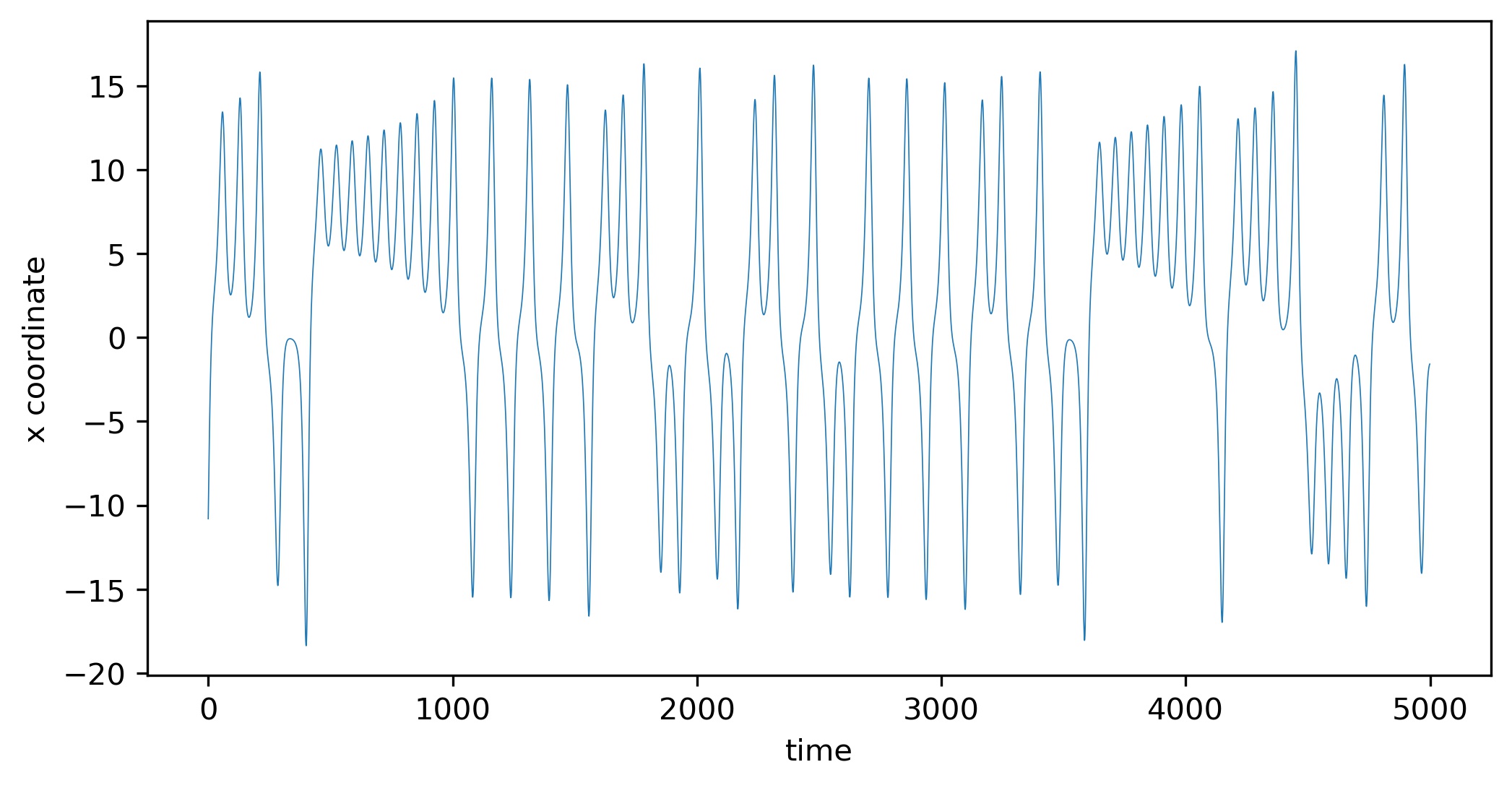
(a)

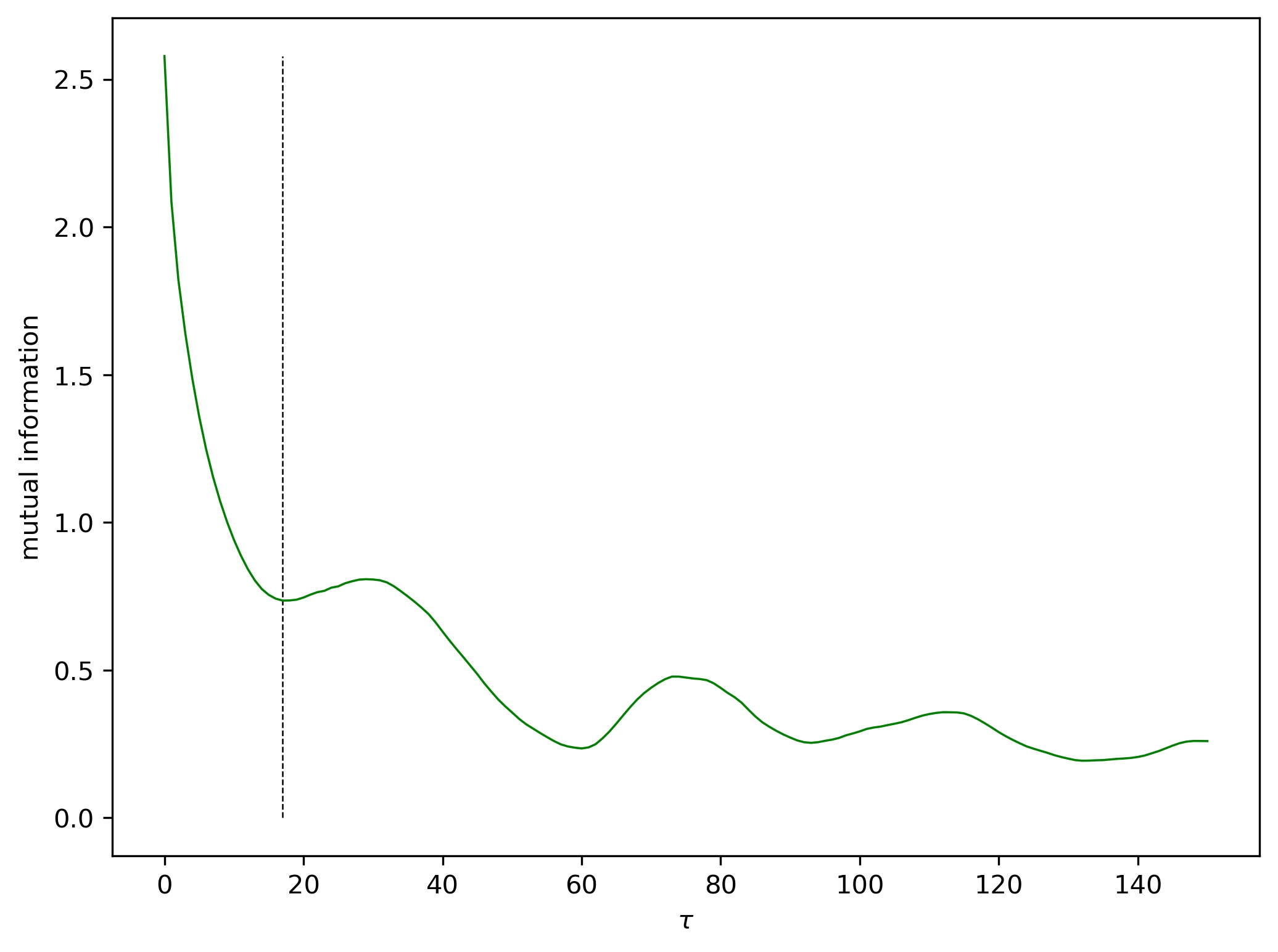
(b)

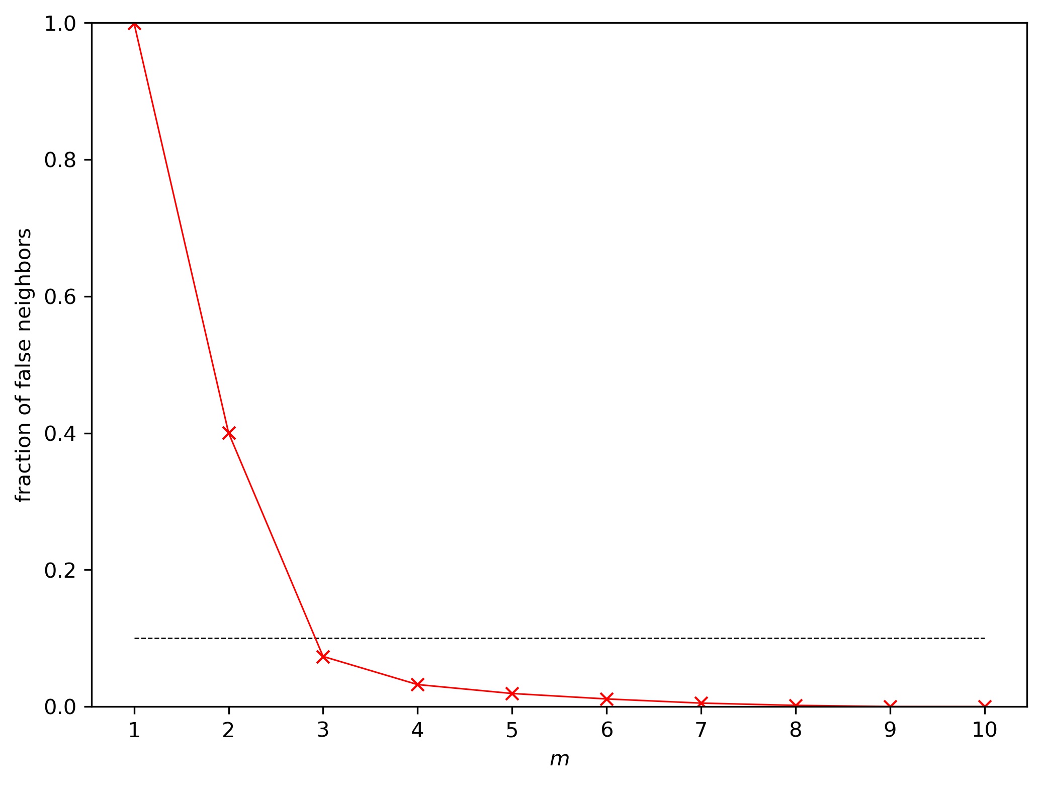
(c)

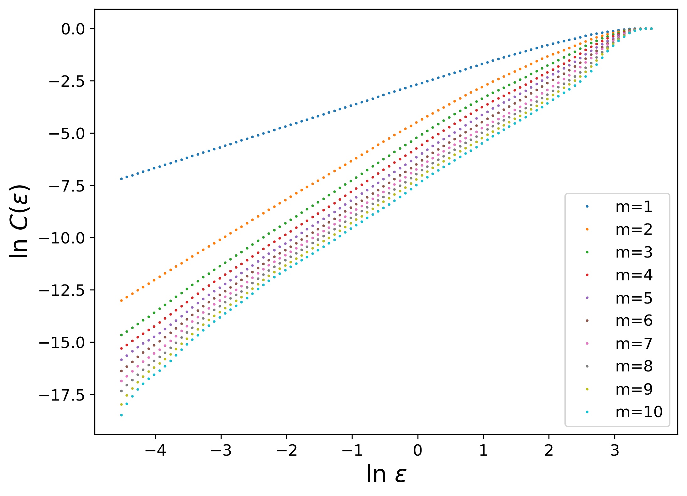
(d)

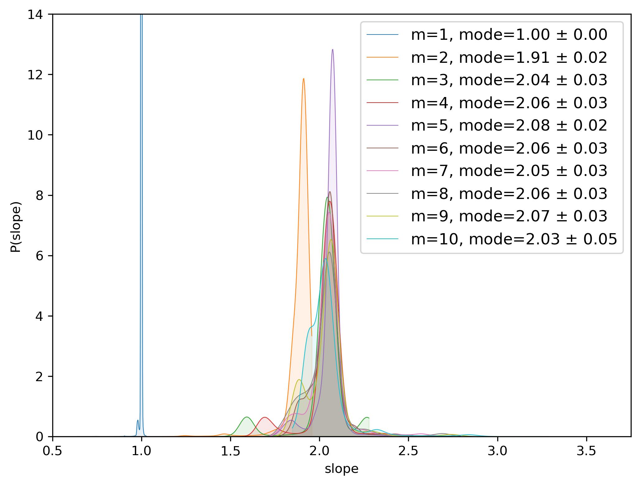
(e)

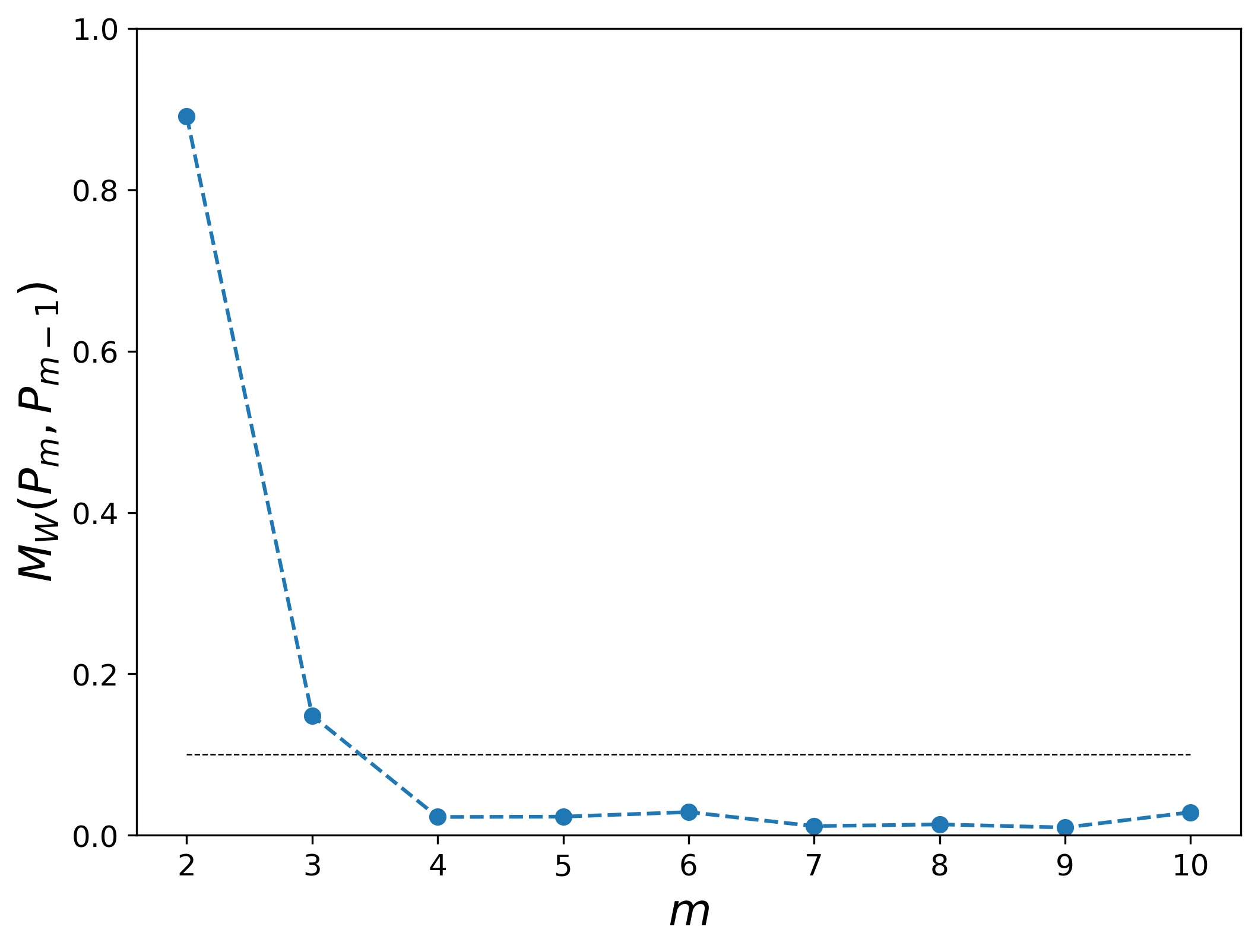
(f)

Figure 1: Extracting a scaling region using an ensemble-based approach (a) Example time series: $x$ coordinate of the Lorenz-63 system. (b) Average mutual information as a function of $\tau$, computed using TISEAN’s mutual command. (c) Percentage of false near neighbors as a function of the embedding dimension $m$, computed with $\tau=18$ using TISEAN’s false_nearest command; (d) Correlation sum plots for embeddings with $\tau=18$ and $m=[1,10]$, computed using TISEAN’s d2 command; (e) Weighted slope distributions generated from an ensemble of fits in different intervals from panel (d). (f) Wasserstein distance between successive slope distributions.

The bottom three panels of Figure 1 demonstrate our methodology using the correlation dimension as an asymptotic invariant. The correlation sums, $C(\epsilon)$, are found from TISEAN’s d2 command for a range of $m$ values. Here $\epsilon$ is the size of the balls used to cover the set during the calculation of the Grassberger-Procaccia algorithm [17]. Panel (d) shows $\ln C(\epsilon)$ versus $\ln\epsilon$. If this plot has a scaling region, its slope is the correlation dimension.

It is common practice to choose the endpoints of a scaling region by eye, and then compute the slope using a linear fit. In this case, if the slopes were to converge as $m$ increases, it is thought that the $m$-embedded attractor is properly unfolded and that the value of the correlation dimension is correct. Figure 1(d) shows clear scaling regions whose slopes behave as expected: when $m$ is too low, the attractor is not properly unfolded, so the correlation dimension—i.e., the slopes of the blue ($m=1$) and orange ($m=2$) traces—is artificially low. As $m$ increases, the slopes increase and then appear to converge.

We formalize this procedure using the method of Deshmukh et al. [7], which uses slope distributions to identify scaling regions and the Wasserstein distance to establish convergence of the distributions with increasing $m$. As a first step, we compute potential scaling regions corresponding to an ensemble of intervals with various values of $\ln(\epsilon)$ for left and right endpoints. We set the minimum number of points for the fitting interval to be $10$, but allow all possible combinations otherwise. This choice is discussed in [7]. For example, in panel (d) there are $100$ possible selections of endpoints, so using a minimal width of $10$ gives $4005$ potential scaling regions. For each $m$ in Figure 1(d), we then generate a distribution of slopes, $P_{m}$, from least-squares fits for each interval. The goodness of the fit is included by weighting each result by the length of the fitting interval and inversely by square of the fit error. We show kernel density estimates for these distributions in panel (e), calculated using python’s scipy.stats.gaussian_kde command.

The geometry of these distributions brings out the salient information quite effectively, including both the existence of one or more scaling regions and their slopes. Unimodal slope distributions, as in Figure 1(e), suggest the presence of a single, wide scaling region for d2. The mode of $P_{m}$ is an estimate of the slope of the scaling region and the width of the distribution around that mode width gives an indication of precision. More formally, we calculate a confidence interval by computing the standard deviation, $\sigma$, of the ensemble members within the full width at half maximum (FWHM) of the mode. For the $m=2$ case (orange), $\sigma=0.02$, giving the estimated slope $1.92\pm 0.02$.

If there were no scaling region in the plot, the distribution would be wide and the corresponding confidence interval large. For Figure 1, the trajectory samples the attractor cleanly and thoroughly, resulting in small error estimates. However, this is not the case for all of the examples below. Moreover, if the plot contains multiple scaling regions, the distributions will be multi-modal. This may occur, for example, for d2 when $\epsilon$ is larger than the diameter of the attractor, or for noisy data when $\epsilon$ is small [7]. The possibility of such multi-modal distributions is why we use the mode rather than the mean.

The choice of the smallest embedding dimension that gives an accurate and valid calculation of the correlation dimension is the critical matter at issue here. We assert that this $m$ corresponds to the smallest value for which the slope distributions “converge.” In Figure 1(d), this convergence is apparent to the eye: the $P_{1}$ (blue) and $P_{2}$ (orange) distributions reflect the low correlation dimensions of an incompletely unfolded attractor; however, the $P_{m}$ for $m\geq 3$ largely overlap. This suggests that $m=3$ or $4$ would be a good choice.

To formalize the notion of convergence, we use the Wasserstein metric [11], $M_{W}$, to compare sequential pairs $P_{m}$ and $P_{m-1}$. As a metric, $M_{W}=0$ if and only if the distributions are identical, or—as we are using it for samples—if and only if the weighted sample values are the same. Figure 1(f) shows $M_{W}(P_{m},P_{m-1})$ for the Lorenz-63 d2 slope distributions, calculated using the python scipy.stats.wasserstein_distance package. For this noise-free, low-dimensional case, the distance $M_{W}(P_{m},P_{m-1})$ montonically decreases with $m$.

For real-valued data, it is known that the $L_{1}$ Wasserstein distance for a sample of size $N$ from a distribution approaches zero as ${N^{-1/2}}$ under some technical assumptions [18]. In our experiments, $N=\mathcal{O}(10^{3})$ is the number of selected left and right endpoint pairs for the linear fits. The theoretical error is also proportional to the width of the PDF, which in our applications tends to be $\mathcal{O}(1)$. We make the null hypothesis that the PDFs are the same if

$$M_{W}(P_{m},P_{m-1})\lesssim 0.1.$$

In Figure 1(f) this threshold, shown as the dashed line, first occurs at $m=4$ where $M_{W}(P_{4},P_{3})=0.025<0.1$, so we choose this embedding dimension. This then gives $d_{2}=2.06\pm 0.03$.

Our approach bears some similarities to other methods for choosing $m$. Our procedure employs a threshold that superficially resembles that used in the FNN method, but the $M_{W}$ threshold is mathematically justifiable. By contrast, there appears to be no such justification for the selection of a threshold for the percentage of false nearest neighbors. The suggestion of [4] is that “a physicist might well choose to accept this threshold to make more efficient any further computations performed on the data,” provides a reason based only on convenience. Moreover, the percentages of FNN can vary widely with $\tau$ and $m$, and also are sensitive to noise [6]. This further complicates the selection of a threshold for the FNN heuristic. Similarly, Cao [19] proposes a method to automate the asymptotic invariant approach by comparing quantities calculated from embeddings at successive dimensions. The quantities are derived from distances between points that are neighbors in space ($E1(d)$) or in time ($E2(d)$). However, the paper does formalize a threshold on $E1$ and $E2$ to indicate that the correct embedding dimension has been reached.

For the second example, we use the Lorenz-96 trajectory described in Section 2.1 to give a time series sampled from an attractor in a 14D state space. In this case, AMI (not shown here) does not give a good estimate for $\tau$ because it has broad, almost-flat region with a first minimum at $\tau=145$, a value that produces an over-folded embedding. Instead, we use the curvature-based heuristic of [20] to select $\tau=23$. The resulting correlation sums from TISEAN for a range of embedding dimensions are shown in Figure 2(a).

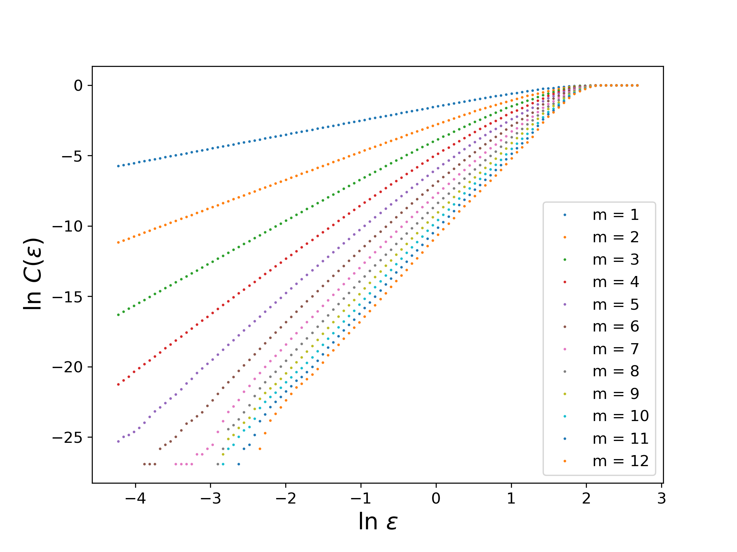
(a)

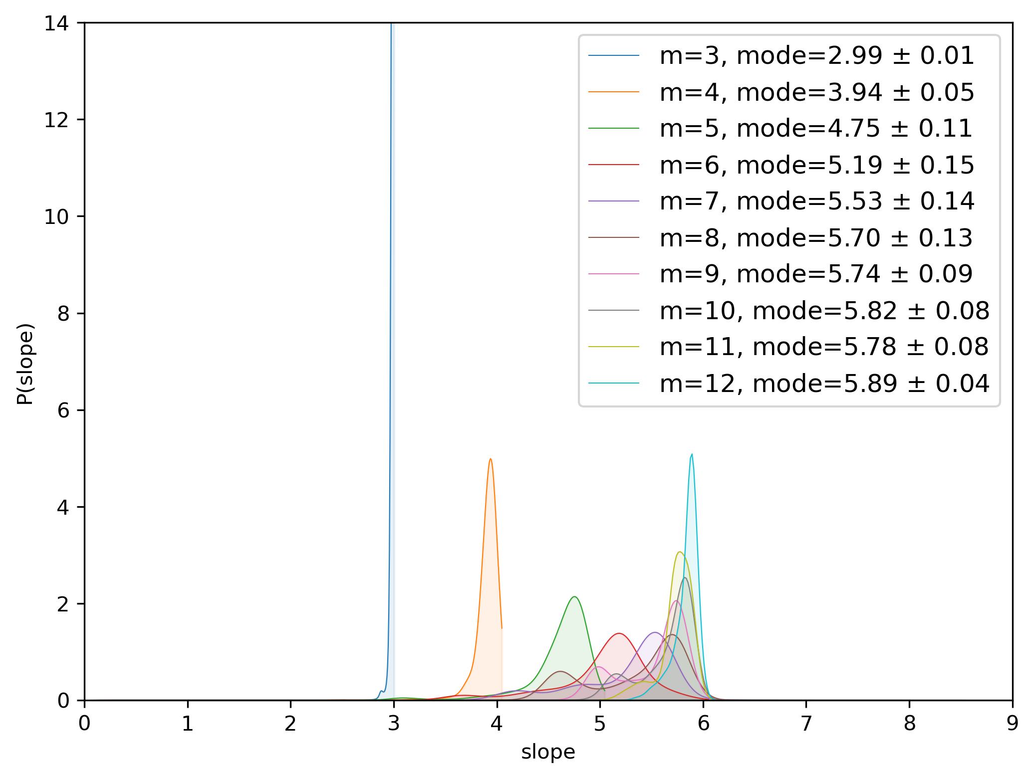
(b)

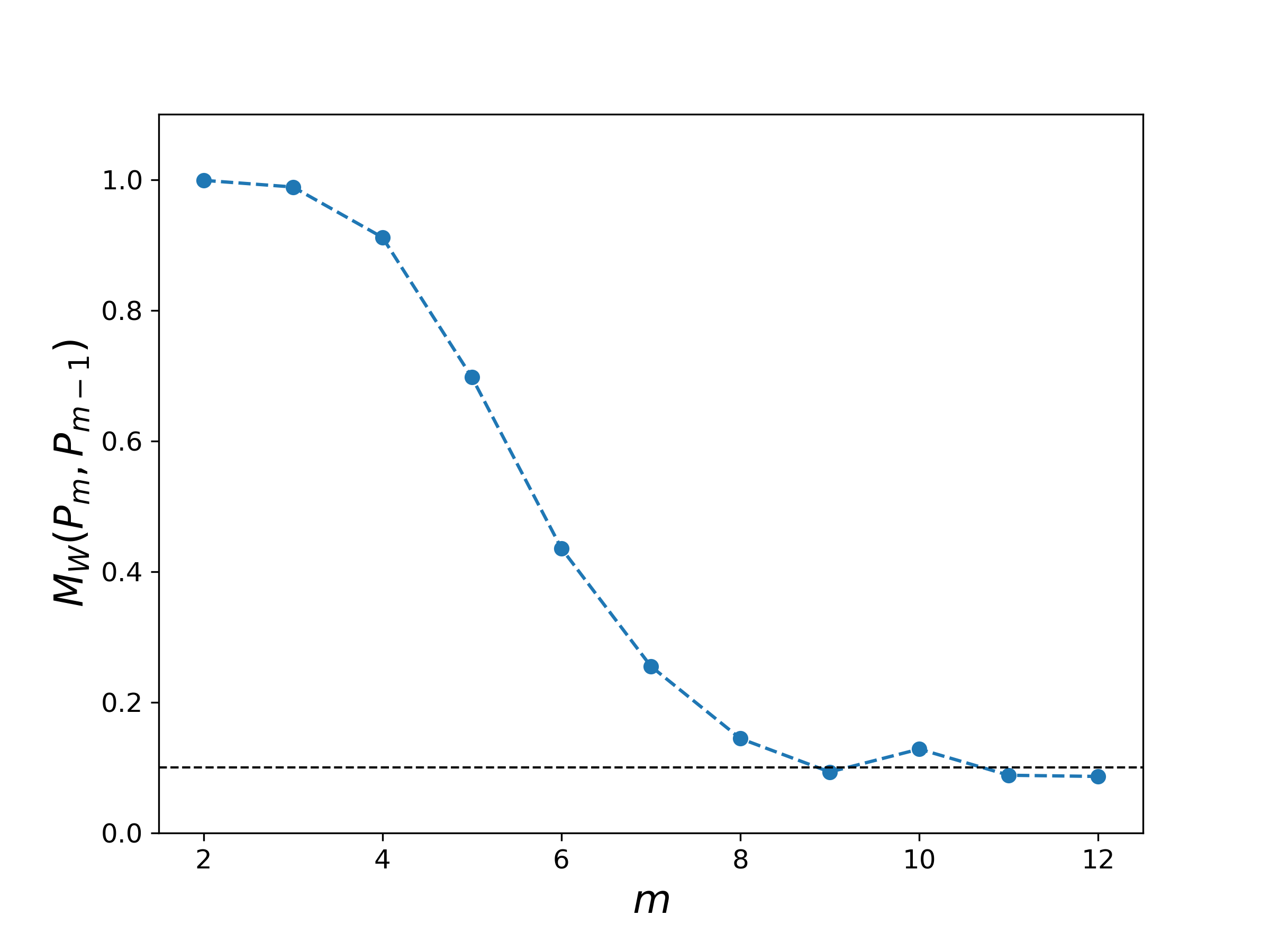
(c)

Figure 2: Lorenz 96 example: (a) Correlation sum plots for embeddings for $\tau=23$ and $m=[3,12]$, computed using TISEAN’s d2 command. (b) Weighted slope distributions generated from an ensemble of fits in different intervals of the plot in (a). (c) Convergence of slope distributions.

The corresponding slope distributions, panel (b), exhibit the same behavior as the Lorenz-63 example: they peak at artificially low slopes when the dimension is too small, and appear to converge with increasing $m$. The Wasserstein plot, panel (c), confirms this and suggests $m=9$ is sufficient. This gives $d_{2}=5.74\pm 0.09$.

For this data set, the FNN method would require a larger value, $m=11$, which gives a slightly larger estimate of the correlation dimension. The difference between the two estimates stems from what each method is trying to do. FNN performs an aggregate calculation of neighbor relationships across the attractor, with the goal of identifying false trajectory crossings created by inadequate unfolding. Elimination of such crossings is sufficient for computing the correct dimension, but not necessary [6]. By contrast, our method uses the convergence of the desired invariant as the primary criterion, which is more appropriate given that this is the goal.

Moving beyond synthetic examples, we now consider two PIC laser data sets from McMahon et al. [16]. These were gathered from the same device but under different conditions and, as noted in the paper, lead to quite different dynamics; see Figure 3(a) and (b).

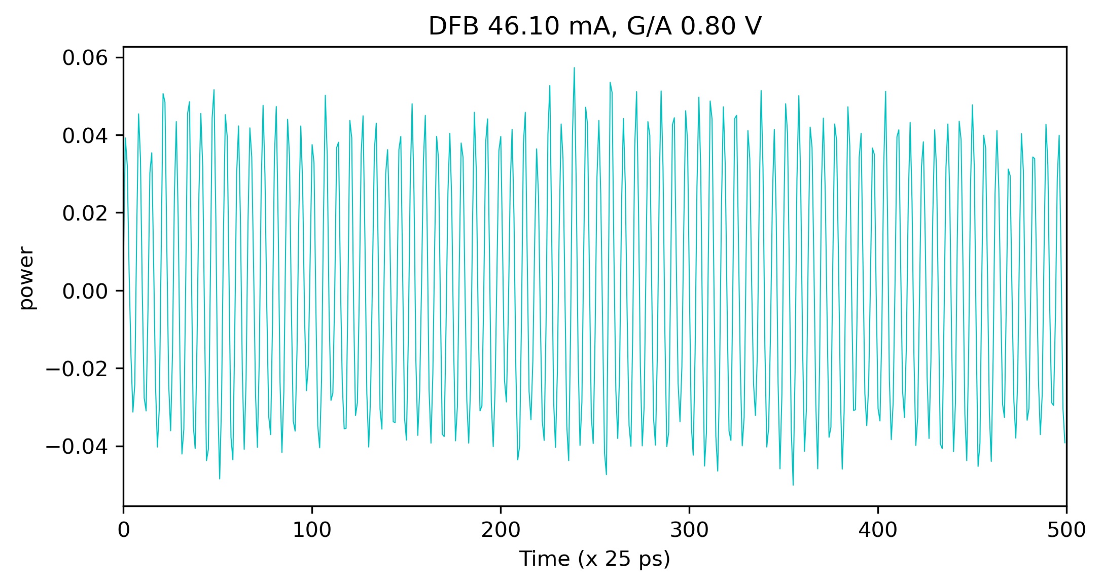
(a)

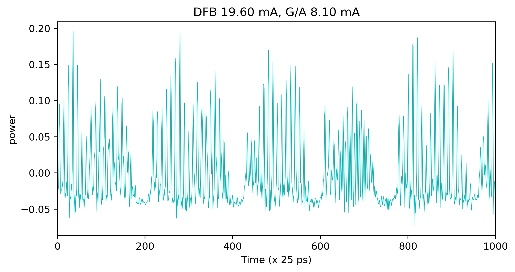
(b)

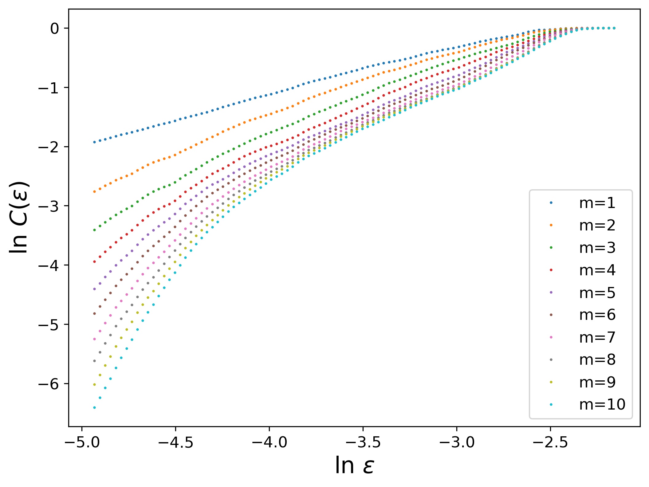
(c)

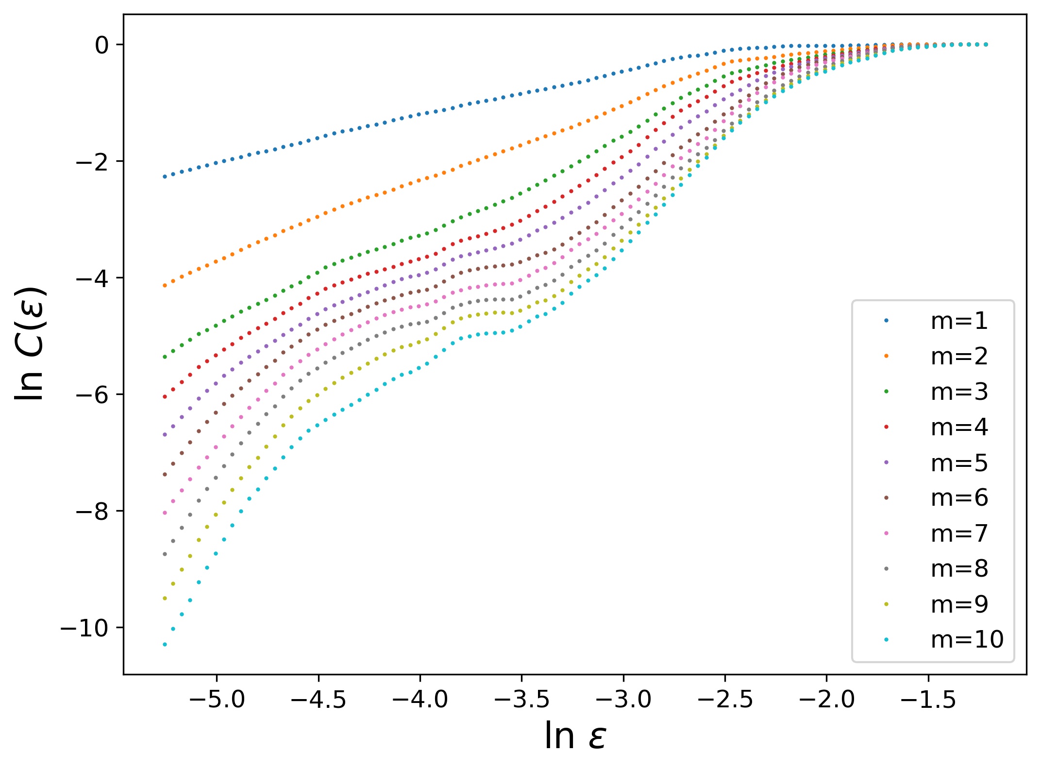
(d)

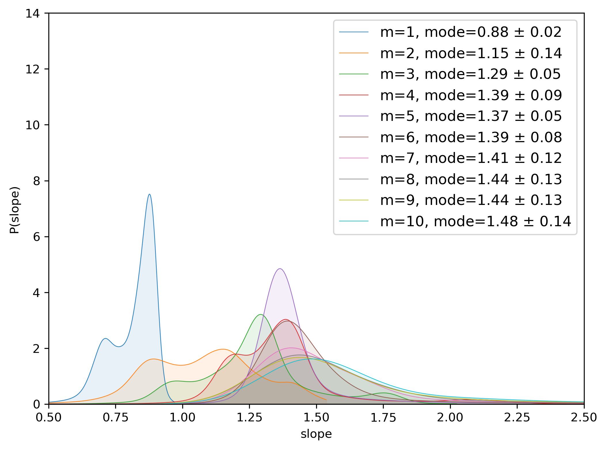
(e)

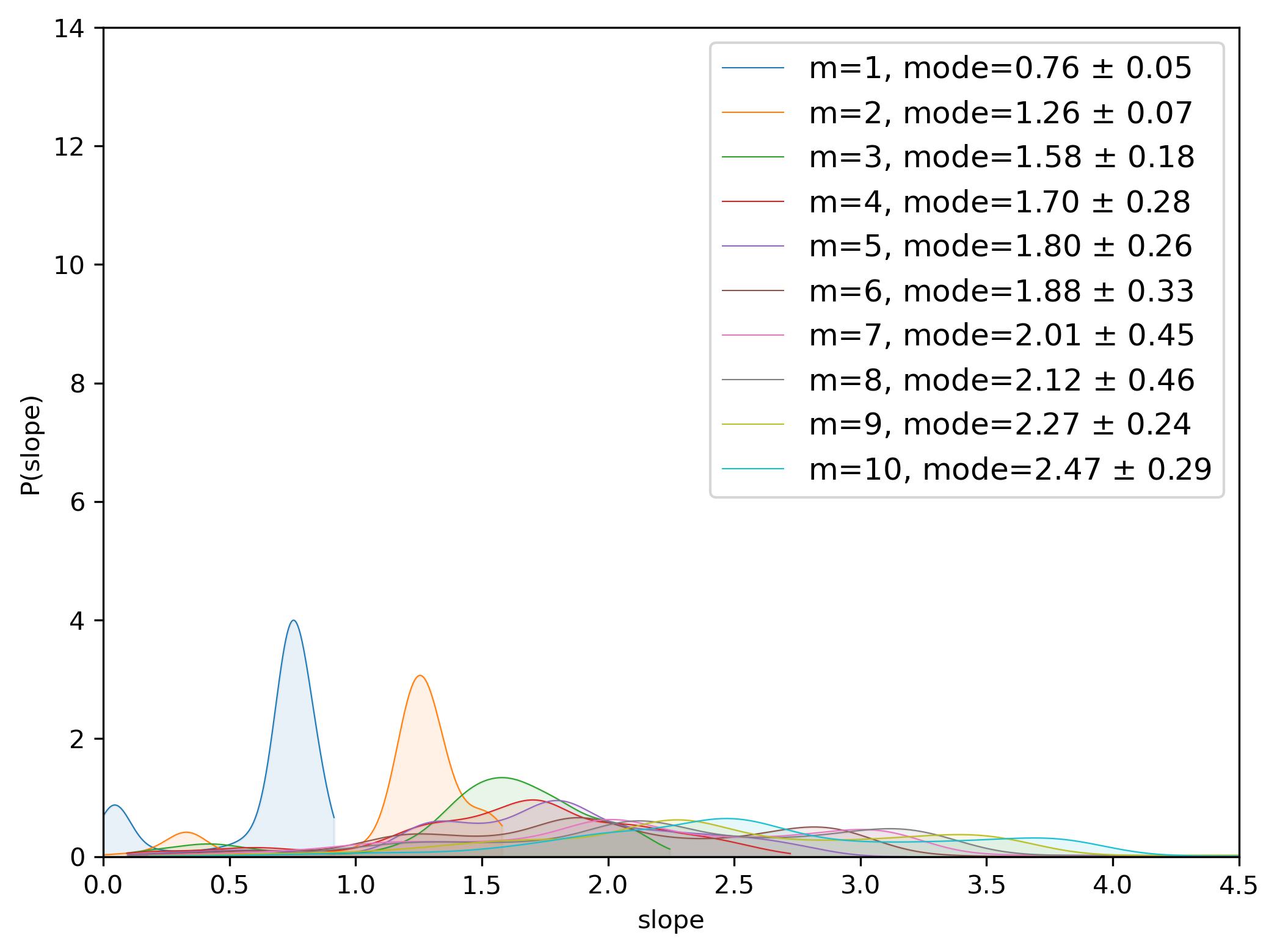
(f)

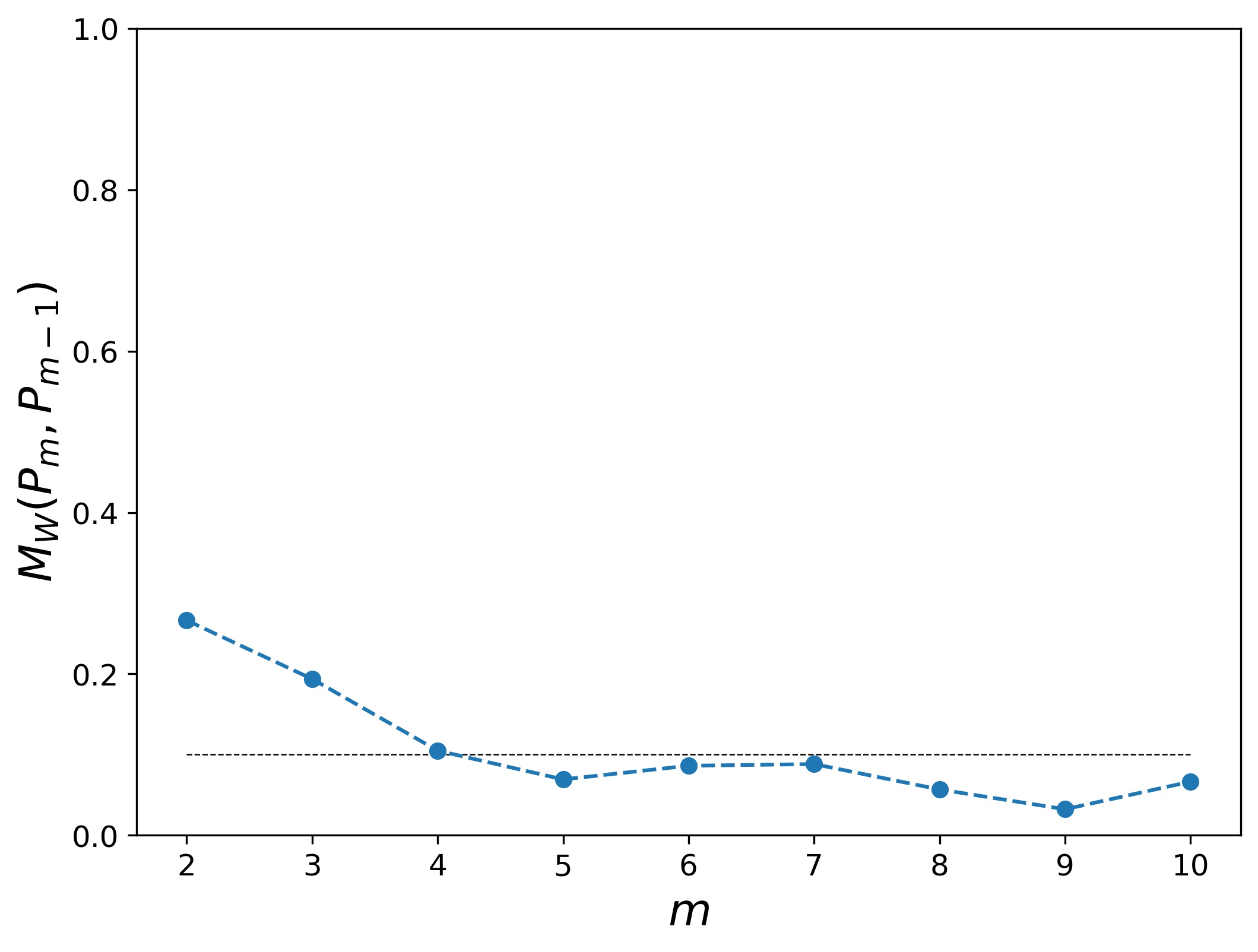
(g)

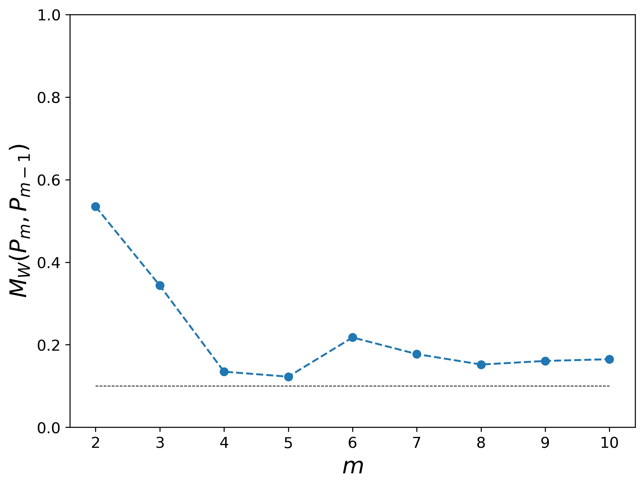
(h)

Figure 3: Extracting scaling regions for data from two laser experiments, segments of which are shown in the top two panels. Below those traces are the correlation sum plots, slope distributions, endpoint distributions, and convergence measures for the corresponding data.

McMahon et al. first estimate $\tau$ using AMI then calculate the correlation sums over a fixed range of $m\in[5,10]$. They apply a “minimum gradient detection” algorithm to find scaling regions. This method gives $d_{2}=1.27\pm 0.05$ and $1.01\pm 0.06$, respectively. The paper does not note a “best” value for $m$, as their goal is calculation of the correlation dimension, not the embedding dimension.

The results of applying our methodology to this data are shown in Figure 3(c)-(h). The AMI method gives $\tau=3$ for both cases. The correlation sum for a range of $m$ values is shown in panels (c) and (d). Panels (e) and (f) show the corresponding slope distributions, and (g) and (h) show the Wasserstein distances. For the data in the left-hand column, the slope distributions are multimodal for $m\in[1,4]$, reflecting the distinct linear regions in panel (c). The PDFs in (e) are far broader than those in Figures 1 and 2, indicating less certainty. Nevertheless, the Wasserstein distance in panel (g) does drop below the $0.1$ threshold for $m=5$, implying $d_{2}=1.26\pm 0.07$. This is in good agreement with the quoted results of McMahon et al., though it should be noted that their confidence interval is calculated differently.

The story is quite different for the second case. The distributions in Figure 3(f) do not appear to converge with increasing $m$; this is corroborated by the Wasserstein metric in panel (h). Indeed, the the curves in panel (d) are clearly problematic from the standpoint of time-series analysis. The $m=1$ and $m=2$ results do have scaling regions—indicated by the strong, unimodal peaks in the blue and orange distributions in panel (f)—but the slopes of these regions give spurious $d_{2}$ values because the attractor is not reconstructed properly for such low dimensions (as is clear from the change in slope with increasing $m$ in this range). When $m>2$, none of the $d_{2}$ curves have clear scaling regions. The slope distributions bring this out clearly: the Wasserstein distance never falls below $0.1$, indicating that low confidence in the correlation dimension. This is not in accord with the asserted value in [16], perhaps because computing a gradient from noisy data—as is done in that paper—is notoriously problematic.

A number of methods have been proposed to automate the estimation of $d_{2}$: see, for example, [21, 22, 23]. These papers essentially use following workflow: calculate a local gradient of the correlation sum, generate a histogram of the slopes, and then locate the peak value. Numerical differentiation can, of course, be problematic unless the data points are noise free. Our method is designed to avoid this issue. Since we weight the linear fits by their length, we favor longer fits, thus de-emphasizing small-scale noise. Our choice of the mode of the slope distribution provides a slope that is common to a range of endpoint choices. Another important difference between our method and that in the cited papers is generality. The primary focus of those papers is an automatic estimate for the correlation dimension. The objective of our method is to select a good value of the embedding dimension; the d2 calculation is only the vehicle. Any other dynamical invariant would be just as good, as we show next.

2.2.2 Other invariants

Correlation dimension is not the only dynamical invariant that involves fitting a line to a scaling region. Another important quantity is the largest Lyapunov exponent, $\lambda_{1}$, as computed by the widely used Kantz [24] and Rosenstein [25] algorithms. These calculate a “stretching factor” $S(\Delta n)$ between nearby trajectory points. This also gives a scaling region to which or method can be applied. This, in turn, provides another opportunity for an automated asymptotic invariant approach to choosing embedding parameter values.

Figure 4 shows the results of this approach, as applied to the Lorenz-63 dataset from Section 2.1 using TISEAN’s lyap_k command.

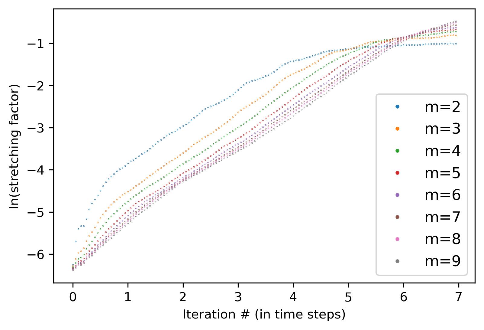
(a)

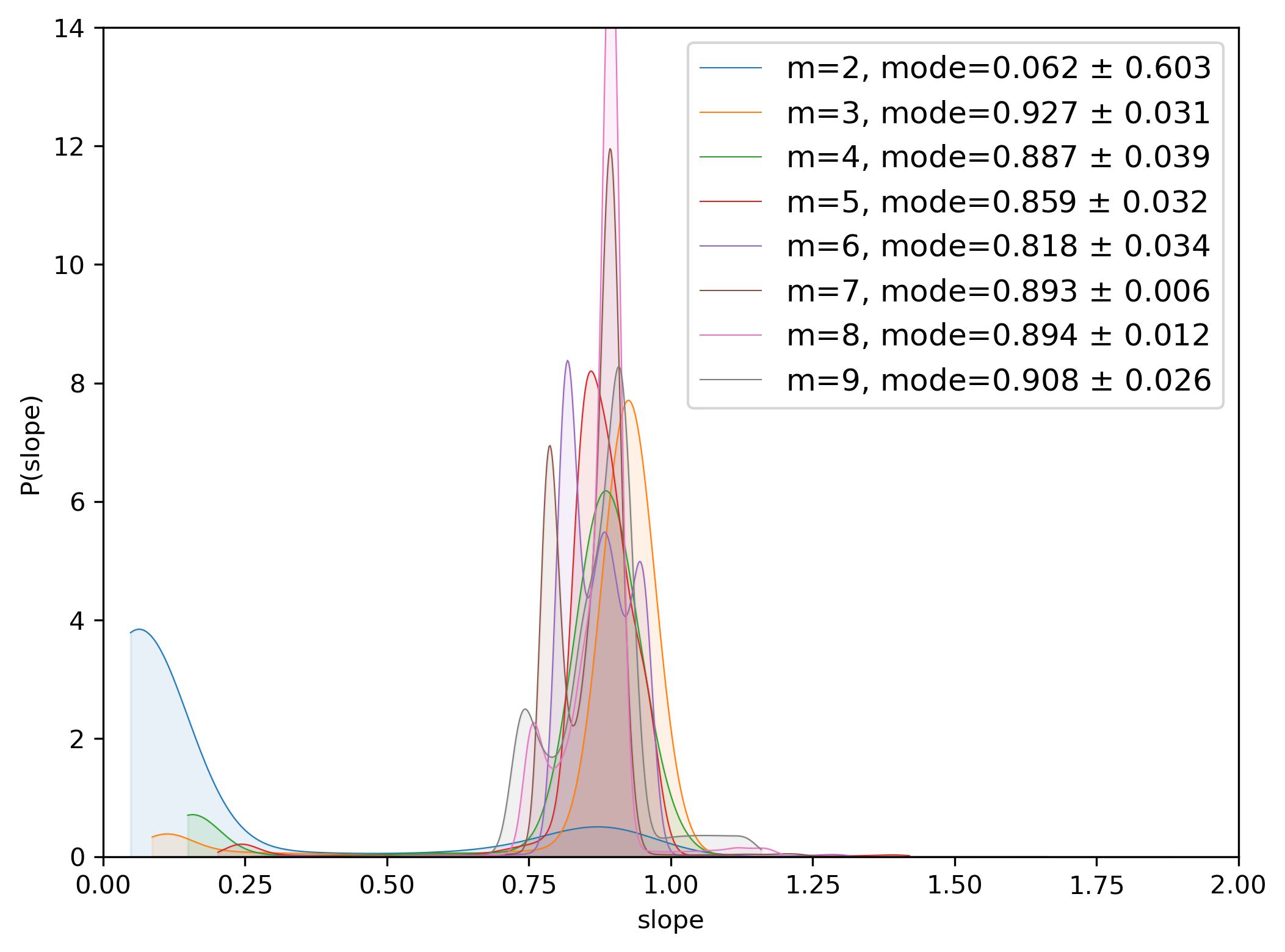
(b)

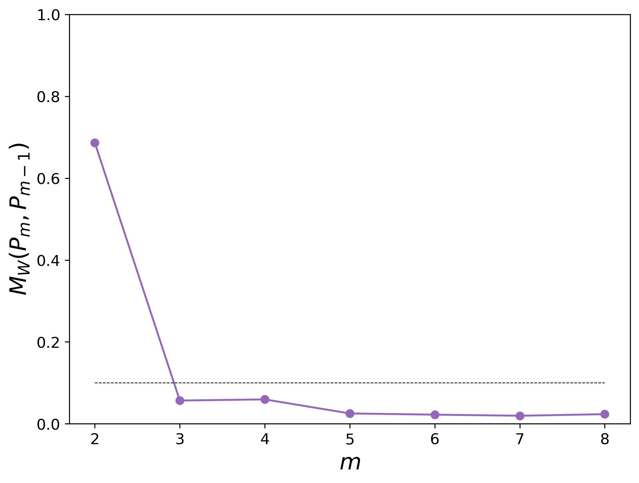
(c)

Figure 4: Asymptotic invariant analysis of the Lorenz-63 system using the largest Lyapunov exponent: (a) spreading factor for embeddings for $\tau=18$ and $m=[2,9]$, computed using TISEAN’s lyap_k command. (b) Weighted slope distributions generated from an ensemble of fits in different intervals of the plots in (a). (c) Convergence of slope distributions.

The Wasserstein plot in panel (c) suggests that $m=3$ is adequate for this computation on this data set. Note that this is smaller than the value of $m=4$ that we obtained using d2 calculations on this trajectory. This brings out an interesting point: different values of the embedding dimension may be sufficient for the calculation of different invariants. This is likely due to a combination of both dynamical and algorithmic effects. The lyap_k algorithm analyzes how the dynamics deform the state space by tracking the forward images of points in an initial $\epsilon$-ball that stretch along the most unstable manifold. Our results suggest that this effect can be tracked effectively in $m=3$, whereas the machinery of the d2 algorithm, which counts points in $m$-dimensional $\epsilon$-balls, requires a more fully unfolded reconstruction. In other words, both the nature of the invariant and the algorithm play a role. This is not the first observation of this effect, of course, see for example, Garland et al. [26].

On a related note: the size of the initial $\epsilon$ ball in the lyap_k calculation is set, by default, to five $1/1000$th and $1/100$th of the span of the data, and $S(\Delta n)$ is computed for each $\epsilon$. Data limitations can make the results quite sensitive to this scale, however, so choosing a good $\epsilon$ value—or knowing whether a choice is good—can be a challenge. Our method can provide some insight in this situation. Figure 5 shows the effect of $\epsilon$ on the Wasserstein distance for the Lorenz-63 data.

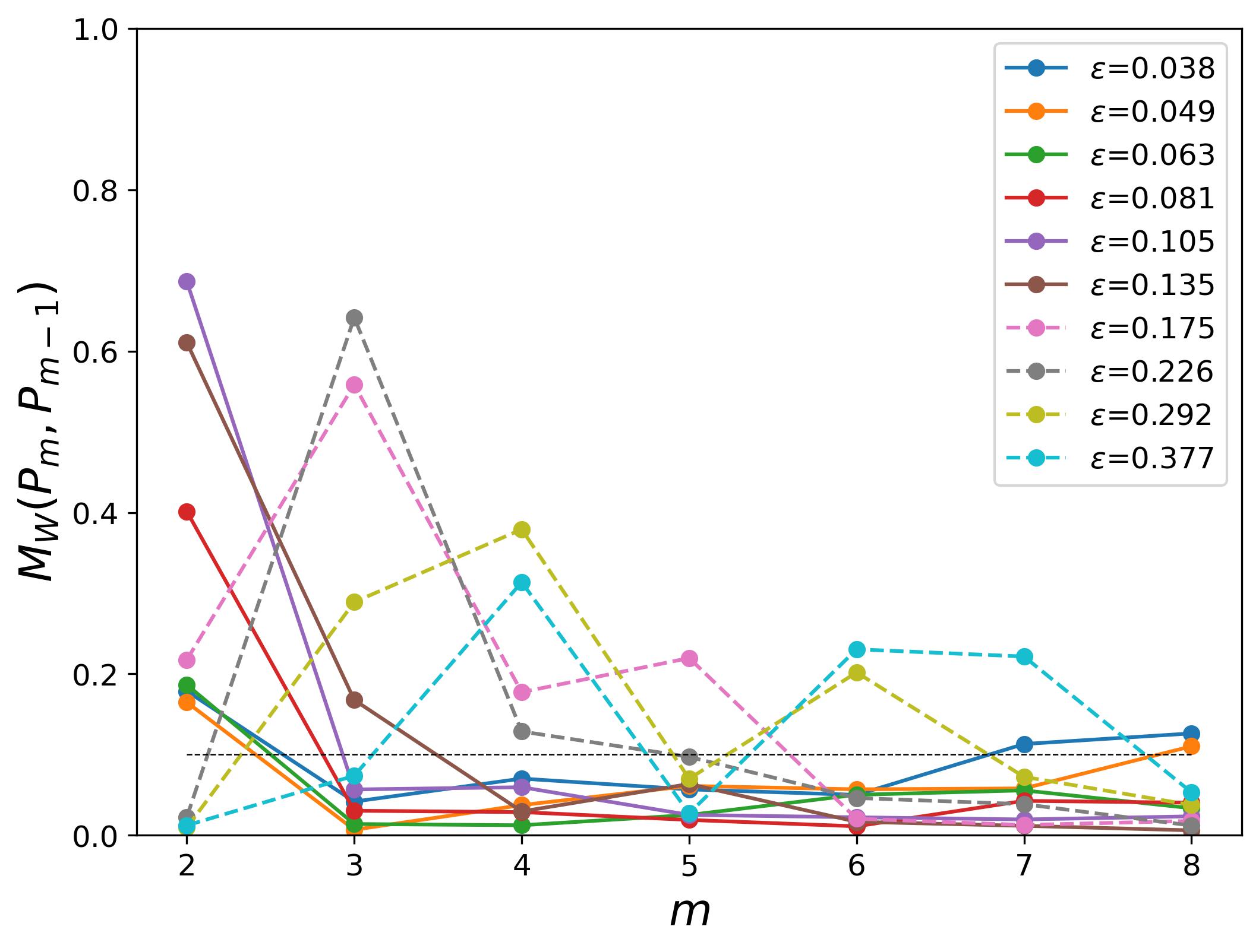
Figure 5: Wasserstein distance for the Lorenz-63 data for a range of $\epsilon$ in the Kantz algorithm for lyap_k. Figure 4(c) uses $\epsilon=0.105$.

For the five smallest values of $\epsilon$, the slopes converge by $m=3$. For $\epsilon=0.135$, the slopes still converge, but not until $m=4$. Beyond that, the Wasserstein distance is non-monotonic, indicating a lack of convergence with increasing dimension. This suggests that this range for $\epsilon$ is problematic.

3 Discussion and conclusion

The choice of the embedding dimension is a critical, but challenging, step in delay reconstruction. As discussed in the last paragraph of Section 2.2.1, a number of good heuristics have been developed to aid in this process. However these do not provide confidence intervals, and all involve subjective thresholds that may or may not be optimal for any particular data set. In the face of this, one might adopt an iterative approach: use some heuristic to obtain a good first guess, then computing some dynamical invariant—e.g., the correlation dimension or Lyapunov exponent—over a range of values for the embedding dimension and looking for convergence. This process, too, can be subjective, as these computations often involve finding, and fitting a slope to, a scaling region. Since this is generally done by eye, it is not immune to confirmation bias.

The contribution of this paper is a method that formalizes and automates this process. We use the ideas of Deshmukh et al. [7] to generate an ensemble of slopes from prospective scaling regions, creating a slope distribution that uses interval width and fit quality as weights. Broad, clean scaling regions manifest as narrow, tall peaks in these distributions. Upon repeating this calculation for a range of embedding dimension, this leads to a good choice $m$ values: when the resulting sequence of slope distributions converges. Convergence is signaled by the decrease of a Wasserstein distance measure below a threshold that is motivated by the theoretical expectation for samples from a fixed distribution. We demonstrated the method in Section 2.2 on data sets from several simulated and experimental examples. We used two dynamical invariants calculated with the TISEAN package: the correlation dimension and the largest Lyapunov exponent. These are obtained from the slope of the correlation sum versus the scale parameter or the stretching factor versus time, respectively. The results corroborate known values, except in one case: a laser data set from [16]. In this case the correlation-sum plots, when examined visually, clearly did not contain true scaling regions.

We emphasize that calculations of such dynamical invariants are valid if—and only if—the plots contain “robust” scaling regions. Robustness is obviously a subjective term that can lead to real problems in the practice of nonlinear time-series analysis. To quote Kantz & Schreiber: “Some authors failed to observe that the curves that they were fitting with straight lines were actually not quite straight…” [27]. Fitting a line blindly to some arbitrarily selected portion of a plot is even worse. A strength of our method is that it objectively measures when there is a scaling region—and, if so, where it is, and what is its slope.

Our technique can also be useful in the invocation of these algorithms. Tools like d2 or lyap_k in the TISEAN package attack a difficult problem: how can one extract dynamical invariants from incomplete samples? These methods involve a number of free parameters such as data length and time scale, the Theiler window [28], etc. The best practice for choosing such parameters mirrors the “asymptotic invariant” approach: vary the parameter, seeking convergence. One can use our method to accomplish this—for individual parameters or even for several at once, using a multivariate sweep. This could include choosing any of the free parameters used in the practice of delay reconstruction.

References

-
[1]
N. Packard, J. P. Crutchfield, J. Farmer, R. Shaw,
Geometry from a time
series, Phys. Rev. Lett. 45 (9) (1980) 712–716.
URL https://doi.org/10.1103/PhysRevLett.45.712 -
[2]
F. Takens, Detecting strange
attractors in fluid turbulence, in: Dynamical systems and turbulence,
Springer, Berlin, 1981, pp. 366–381.
URL https://doi.org/10.1007/BFb0091924 -
[3]
A. Fraser, H. Swinney,
Independent coordinates for
strange attractors from mutual information, Phys. Rev. A 33 (2) (1986)
1134–1140.
URL https://doi.org/10.1103/PhysRevA.33.1134 -
[4]
M. Kennel, R. Brown, H. Abarbanel,
Determining minimum embedding
dimension using a geometrical construction, Phys. Rev. A 45 (6) (1992)
3403–3411.
URL https://doi.org/10.1103/PhysRevA.45.3403 -
[5]
K. Beyer, J. Goldstein, U. Shaft,
When is ‘nearest
neighbor’ meaningful?, in: C. Beeri, P. Buneman (Eds.), Database
Theory—ICDT’99, Vol. 1540 of Lecture Notes in Computer Science,
Springer, Berlin, 1999, p. 217–235.
URL https://doi.org/10.1007/3-540-49257-7_15 -
[6]
A. Krakovská, K. Mezeiová, H. Budáčová,
Use of false nearest neighbours
for selecting variables and embedding parameters for state space
reconstruction, Journal of Complex Systems 2015 (2015) 932750.
URL https://doi.org/10.1155/2015/932750 -
[7]
V. Deshmukh, E. Bradley, J. Garland, J. D. Meiss,
Towards automated extraction and
characterization of scaling regions in dynamical systems, Chaos 31 (2021)
123102.
URL https://doi.org/10.1063/5.0069365 -
[8]
L. Pecora, L. Moniz, J. Nichols, T. Carroll,
A unified approach to attractor
reconstruction, Chaos 17 (1) (2007) 013110.
URL https://doi.org/10.1063/1.2430294 -
[9]
R. Hegger, H. Kantz, T. Schreiber,
Practical implementation of nonlinear
time series methods: The TISEAN package., Chaos 9 (2) (1999) 413–435.
doi:10.1063/1.166424.
URL https://doi.org/10.1063/1.166424 -
[10]
R. Hegger, H. Kantz, T. Schreiber,
Tisean 3.0.1
nonlinear time series analysis (2007).
URL https://www.pks.mpg.de/~tisean/Tisean_3.0.1/index.html -
[11]
S. S. Vallender, Calculation of the
Wasserstein distance between probability distributions on the line, Theory
of Probability & Its Applications 18 (4) (1974) 784–786.
doi:10.1137/1118101.
URL https://doi.org/10.1137/1118101 -
[12]
E. Lorenz,
Deterministic
nonperiodic flow, J. the Atmospheric Sciences 20 (2) (1963) 130–141.
URL https://doi.org/10.1175/1520-0469(1963)020<0130:DNF>2.0.CO;2 - [13] J. C. Sprott, Chaos and time-series analysis, Vol. 69, Oxford University Press, 2003.
- [14] A. Wolf, J. B. Swift, H. L. Swinney, J. A. Vastano, Determining Lyapunov exponents from a time series, Physica D 16 (3) (1985) 285–317.
-
[15]
E. Lorenz, Predictability:
A problem partly solved, in: Predictability of Weather and Climate,
Cambridge University Press, 2006, pp. 40–58.
URL https://doi.org/10.1017/CBO9780511617652.004 -
[16]
C. J. McMahon, J. P. Toomey, D. M. Kane,
Insights on correlation
dimension from dynamics mapping of three experimental nonlinear laser
systems, PLOS ONE 12 (8) (2017) 1–27.
doi:10.1371/journal.pone.0181559.
URL https://doi.org/10.1371/journal.pone.0181559 -
[17]
P. Grassberger, I. Procaccia,
Measuring the
strangeness of strange attractors, Physica D 9 (1-2) (1983) 189–208.
URL https://doi.org/10.1016/0167-2789(83)90298-1 -
[18]
E. del Barrio, E. Gine, C. Matran,
Central limit theorems for the
Wasserstein distance between the empirical and the true distributions,
Annals of Probability 27 (2) (1999) 1009–1071.
URL https://doi.org/10.1214/aop/1022677394 -
[19]
L. Cao, Practical method
for determining the minimum embedding dimension of a scalar time series,
Physica D 110 (1-2) (1997) 43–50.
URL https://doi.org/10.1016/S0167-2789(97)00118-8 -
[20]
V. Deshmukh, E. Bradley, J. Garland, J. D. Meiss,
Using curvature to select the time
lag for delay reconstruction, Chaos: An Interdisciplinary Journal of
Nonlinear Science 30 (6) (2020) 063143.
doi:10.1063/5.0005890.
URL https://doi.org/10.1063/5.0005890 -
[21]
J. P. Toomey, D. M. Kane, S. Valling, A. M. Lindberg,
Automated correlation dimension
analysis of optically injected solid state lasers, Opt. Express 17 (9)
(2009) 7592–7608.
doi:10.1364/OE.17.007592.
URL https://doi.org/10.1364/OE.17.007592 -
[22]
A. Corana, G. Bortolan, A. Casaleggio,
Most probable dimension
value and most flat interval methods for automatic estimation of dimension
from time series, Chaos, Solitons & Fractals 20 (4) (2004) 779–790.
doi:https://doi.org/10.1016/j.chaos.2003.08.012.
URL https://doi.org/10.1016/j.chaos.2003.08.012 -
[23]
A. Casaleggio, G. Bortolan,
Automatic estimation of the
correlation dimension for the analysis of electrocardiograms, Biological
Cybernetics 81 (4) (1999) 279–290.
URL https://doi.org/10.1007/s004220050562 -
[24]
H. Kantz, A robust method
to estimate the maximal Lyapunov exponent of a time series, Phys. Lett. A
185 (1994) 77.
URL https://doi.org/10.1016/0375-9601(94)90991-1 -
[25]
M. Rosenstein, J. Collins, C. J. De Luca,
A
practical method for calculating largest Lyapunov exponents from small data
sets, Physica D 65 (1) (1993) 117–134.
doi:https://doi.org/10.1016/0167-2789(93)90009-P.
URL https://www.sciencedirect.com/science/article/pii/016727899390009P -
[26]
J. Garland, E. Bradley, Prediction in
projection, Chaos 25 (2015) 123108.
URL https://doi.org/10.1063/1.4936242 - [27] H. Kantz, T. Schreiber, Nonlinear Time Series Analysis, Cambridge University Press, Cambridge, 1997.
-
[28]
J. Theiler, Spurious dimension
from correlation algorithms applied to limited time series data, Phys. Rev.
E 34 (3) (1986) 2427–2432.
URL https://doi.org/10.1103/PhysRevA.34.2427