Localisation of Dirac eigenmodes and confinement in gauge theories: the Roberge-Weiss transition

Abstract

Ample numerical evidence from lattice calculations shows a strong connection between the confining properties of gauge theories at finite temperature and the localisation properties of the low-lying Dirac eigenmodes. In this contribution we discuss recent progress on this topic, focussing on results for QCD at imaginary chemical potential ${\mu}_{I}/T=\pi$ at temperatures above the Roberge-Weiss transition temperature. These confirm the general picture of low modes turning from delocalised to localised at the deconfinement transition, in a previously unexplored setup with a genuine, physical transition in the presence of dynamical fermions. This further supports the use of Dirac eigenmodes as a tool to investigate the mechanisms behind confinement and the deconfinement transition.

1 Introduction

While the crossover nature and the location of the QCD transition at finite temperature have been firmly established, the mechanism that drives it is still a matter of active research. In particular, one would like to understand why both confining and chiral properties change dramatically in the same relatively narrow temperature range, where quarks and gluons deconfine and chiral symmetry gets restored. In fact, linear confinement of quarks and spontaneous breaking of chiral symmetry apply to QCD only in an approximate sense, originating from opposite quark mass limits, and it is not yet fully understood how they affect each other.

Quarks are confined by a linear potential only in the “quenched” limit of infinite quark mass, where QCD reduces to pure SU(3) gauge theory. In this setting, deconfinement is signalled by the spontaneous breaking of the exact centre symmetry of the theory by the ordering of the local Polyakov loops, resulting in a vanishing string tension. The Polyakov loop,

$$P(\vec{x}\mkern 2.0mu)=\textrm{Pexp}\left\{ig\int_{0}^{\frac{1}{T}}dt\,A_{4}(t,\vec{x}\mkern 2.0mu)\right\}\,,$$ (1)

is the holonomy of the gauge field around the temporal direction, which in the imaginary-time formulation of finite-temperature gauge theories is compactified to a circle of size equal to the inverse of the temperature, $T$. In pure gauge theory at high temperature the local Polyakov loops tend to align to one of the elements of the gauge group centre, $\mathbb{Z}_{3}$, thus breaking centre symmetry, with the trivial element being the one selected when pure gauge theory is approached as the quenched limit of QCD. Deconfinement is then associated with the ordering of local Polyakov loops, and while to a small extent this is present in QCD already at low temperatures, it becomes considerably stronger at the crossover.

On the other hand, chiral symmetry is a symmetry only in the limit of massless quarks, and only there one can speak of its spontaneous breaking in a strict sense. In this limit, chiral symmetry is spontaneously broken to its vector part by a quark condensate, resulting from the accumulation of eigenvalues of the Dirac operator $\not{D}$ near the origin. This is made clear by the Banks-Casher formula Banks:1979yr ,

$$\Sigma=|\langle\bar{\psi}\psi\rangle|=\int_{0}^{\infty}d\lambda\,\rho(\lambda)\frac{2m}{\lambda^{2}+m^{2}}\,,\qquad\rho(\lambda)\equiv\lim_{V\to\infty}\frac{T}{V}\Big{\langle}\sum_{n}\delta(\lambda-\lambda_{n})\Big{\rangle}\,,$$ (2)

where $\rho(\lambda)$ is the spectral density of $\not{D}$. Here angular brackets denote the expectation value in the sense of the Euclidean functional integral in the imaginary-time formulation of finite-temperature gauge theories, $i\lambda_{n}$ are the eigenvalues of $\not{D}$ in a given gauge configuration, and $V$ is the spatial volume of the system. In the chiral limit one finds precisely $\Sigma\to\pi\rho(0^{+})$. Even for physical quark masses, the crossover is characterised by a dramatic reduction of the density of near-zero modes, and so the approximate restoration of chiral symmetry is signalled by the depletion of the near-zero spectral region.

Despite their very different origins, deconfinement and chiral restoration show a close relationship not only in QCD, but also in other QCD-like gauge theories. In theories with a single, genuine deconfining phase transition (e.g., pure gauge theory, or lattice QCD with $N_{f}=3$ staggered fermions on coarse lattices Karsch:2001nf ), this is associated with a general improvement of the chiral properties, in particular with a decrease of the chiral condensate. In theories with two genuine transitions (e.g., QCD with $N_{f}=2$ adjoint fermions Karsch:1998qj ), deconfinement preceeds chiral restoration. This suggests that deconfinement strongly affects the chiral properties of the theory, although it is not yet clear by means of what mechanism.

What could play a role in this mechanism is the localisation of the low-lying Dirac modes taking place at the finite temperature transition in QCD GarciaGarcia:2006gr ; Kovacs:2012zq ; Cossu:2016scb ; Holicki:2018sms ; Giordano:2013taa ; Nishigaki:2013uya ; Ujfalusi:2015nha and other gauge theories (see Ref. Giordano:2021qav for a recent review). While delocalised at low $T$, low Dirac modes become localised above the transition, up to a critical point in the spectrum known as mobility edge. Ample numerical evidence shows that the connection between deconfinement and low-mode localisation is a general feature of gauge theories. In particular, localised low modes appear precisely at deconfinement when this takes place through a genuine phase transition. The general connection between deconfinement and low-mode localisation is understood qualitatively in terms of the “sea/islands” picture of localisation Bruckmann:2011cc ; Giordano:2015vla ; Giordano:2016cjs ; Giordano:2016vhx . In this picture, the ordering of local Polyakov loops into a “sea”, that signals deconfinement, is responsible for the opening of a gap in the spectrum of $\not{D}$, that can be filled by eigenmodes only at the price of localising on “islands” of Polyakov-loop fluctuations. This leads one to expect the localisation of low Dirac modes in the deconfined phase of a generic gauge theory, an expectation so far supported by all the available numerical investigations Giordano:2021qav .

Until recently, the numerical evidence for a strong deconfinement/localisation connection, with localised modes appearing right at the critical temperature, came mostly from pure gauge theories with a sharp transition. The only exception was the toy model for QCD provided by $N_{f}=3$ staggered fermions on coarse lattices Giordano:2016nuu , where the transition is only a lattice artefact and does not survive the continuum limit. The first study in a theory with a genuine and physical phase transition in the presence of dynamical fermions was done by us in Ref. Cardinali:2021fpu , looking at the Roberge-Weiss transition in QCD with an imaginary chemical potential $\mu_{I}$ at $\hat{\mu}_{I}\equiv\mu_{I}/T=\pi$. Our results confirm the general expectation, and further support the strong connection between deconfinement and localisation.

In this contribution, after a brief review of localisation in Sec. 2, of the sea/islands picture in Sec. 3, and of QCD at finite imaginary chemical potential in Sec. 4, we discuss our results obtained in QCD at $\hat{\mu}_{I}=\pi$ above the Roberge-Weiss temperature in Sec. 5.

2 Localisation

Eigenmode localisation is a concept originating in the study of random Hamiltonians mimicking disordered systems lee1985disordered . Qualitatively speaking, the localised modes of a random Hamiltonian $H$ are those supported essentially only in a finite region of space, where their amplitude squared $\|\psi(x)\|^{2}=\sum_{\alpha}\psi_{\alpha}(x)^{*}\psi_{\alpha}(x)$ is not negligible, $\|\psi(x)\|^{2}\sim 1/L_{0}^{d}$ with $d$ the spatial dimension and $L_{0}$ the linear size of the localisation region. Here $\sum_{\alpha}$ denotes the sum over any discrete spacetime or internal index. Delocalised modes instead extend throughout the system, with $\|\psi(x)\|^{2}\sim 1/L^{d}$ in a finite spatial box of side $L$. A more accurate characterisation is in terms of how the average spatial size of the modes scales with the system size. This is obtained from their inverse partecipation ratio (IPR), averaged over modes in the spectral region of interest and over realisations of $H$,

$$\overline{\textrm{IPR}}(\lambda,L)=\frac{\langle\sum_{n}\delta(\lambda-\lambda_{n})\textrm{IPR}_{n}\rangle}{\langle\sum_{n}\delta(\lambda-\lambda_{n})\rangle}\,,\qquad\textrm{IPR}_{n}=\int d^{d}x\,\|\psi_{n}(x)\|^{4}\,,$$ (3)

where $\psi_{n}$ and $\lambda_{n}$ are the eigenmodes and eigenvalues of $H$ for some disorder realisation, $H\psi_{n}=\lambda_{n}\psi_{n}$, and angular brackets indicate the average over disorder. The inverse of the IPR measures the spatial size of the mode: for localised modes $\overline{\textrm{IPR}}(\lambda,L)$ remains finite as $L\to\infty$, while for delocalised modes $\overline{\textrm{IPR}}(\lambda,L)\to 0$.

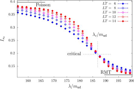
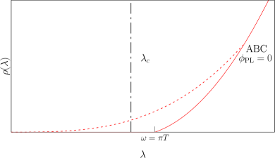
Figure 1: Left: $I_{s_{0}}$ [see Eq. (5)] along the Dirac spectrum (in units of the light-quark mass $m_{\textrm{ud}}$) for 2+1 flavour lattice QCD at $T=394\leavevmode\nobreak\ \textrm{MeV}$, for several spatial sizes $L$ (here the lattice spacing is $a=0.125\leavevmode\nobreak\ \textrm{fm}$, and $s_{0}\simeq 0.508$). The mobility edge, the critical value of the statistics, as well as the Poisson and RMT expectations are also shown. (Data from Ref. Giordano:2013taa .) Right: Sketch of the spectral density in high-temperature QCD ($\hat{\mu}_{I}=0$). The solid line is the spectral density in the case of vanishing gauge fields, starting at the gap $\omega=\pi T$, while the dashed line qualitatively shows the spectral density after the inclusion of localised modes penetrating the gap, and $\lambda_{c}$ indicates the position of the mobility edge.

A convenient way to detect localisation is through the study of the statistical properties of the eigenvalues altshuler1986repulsion . Since delocalised modes are easily mixed by disorder fluctuations, the corresponding eigenvalues are expected to obey the statistics of the appropriate ensemble of Random Matrix Theory (RMT) mehta2004random , depending on the symmetry class of $H$. Localised modes, on the other hand, are sensitive only to disorder fluctuations in their localisation region, and so the corresponding eigenvalues should fluctuate independently for uncorrelated disorder, or more generally for disorder with short-range correlations, therefore obeying Poisson statistics. A simple way to analyse the statistical properties of the spectrum is in terms of the distribution $p_{\lambda}(s)$ of the unfolded level spacings, computed locally in the spectrum. Unfolded level spacings are defined as

$$s_{i}=\frac{\lambda_{i+1}-\lambda_{i}}{\langle\lambda_{n+1}-\lambda_{n}\rangle_{\lambda}}\,,$$ (4)

where ${\langle\lambda_{n+1}-\lambda_{n}\rangle_{\lambda}}$ is the average level spacing in the spectral region of interest. The behaviour of $p_{\lambda}(s)$ is universal, depending only on the type of statistics and not on the details of the model, and is explicitly known both for Poisson and RMT statistics. Localisation can then be detected by comparing features of $p_{\lambda}(s)$ to the known expectations. To this end, a particularly convenient observable is the integrated unfolded level spacing distribution Shklovskii:1993zz

$$I_{s_{0}}=\int_{0}^{s_{0}}ds\,p_{\lambda}(s)\,,$$ (5)

where $s_{0}$ is chosen to maximise the difference between the Poisson and RMT expectations.

Disordered systems typically display disjoint spectral regions of localised and delocalised modes separated by mobility edges, where the localisation length of the localised modes diverges and the system undergoes a second-order phase transition known as Anderson transition Evers:2008zz . As the system size increases, observables like $I_{s_{0}}$ tend to their Poisson or RMT expectation depending on the localisation properties of the modes in the spectral region of interest, except at a mobility edge, where they are scale-invariant and take the critical value appropriate for the symmetry class of the system. This allows for an accurate determination of the position of the mobility edge via a finite-size scaling analysis or, if the critical value is known, by looking for the point where the observable takes it.

The discussion above carries over unchanged to the study of the eigenmodes of the Dirac operator, which is precisely ($-i$ times) a random Hamiltonian with disorder provided by the fluctuations of the gauge fields, over which one integrates in the functional-integral formulation of the theory. An example of how to detect localisation of Dirac eigenmodes using spectral statistics is shown in Fig. 1 (left), in the case of high-temperature lattice QCD. The volume tendency of $I_{s_{0}}$ is clear, and the scale-invariant point, i.e., the mobility edge, is easily spotted.

The presence of localised modes in the spectrum of $\not{D}$ in QCD is by itself not surprising given the formal analogy with random Hamiltonians. Similarly, it is not surprising that critical properties at the mobility edge match those of the 3D unitary Anderson model Hamiltonian Giordano:2013taa ; Nishigaki:2013uya ; Ujfalusi:2015nha , which has the same dimensionality and symmetry class as $\not{D}$ in QCD. What is surprising though, and calls for an explanation, is the sudden appearance of localised modes near the origin at sufficiently high temperatures.

3 Sea/islands picture

A qualitative explanation of localisation in QCD was proposed in Ref. Bruckmann:2011cc and refined in Refs. Giordano:2015vla ; Giordano:2016cjs ; Giordano:2016vhx . This is based on the observation that the local Polyakov loop acts in practice as a space-dependent effective temporal boundary condition for the Dirac eigenmodes, modifying the “twist” on the wave functions coming from the antiperiodic boundary conditions. At high temperature in the deconfined phase the Polyakov loops get ordered, and so doing they induce strong correlations in the temporal direction. In a first approximation one can then imagine the typical gauge configurations as fluctuating around a strongly ordered configuration with identical Polyakov loops $P(\vec{x}\mkern 2.0mu)=\textrm{diag}(e^{i\phi_{a}})$, $\phi_{a}\in(-\pi,\pi]$, and trivial spatial gauge fields. For this kind of configuration the eigenmodes and the spectrum can be computed exactly: eigenmodes are delocalised plane waves, and the spectrum has a gap $\omega(\phi_{\textrm{PL}})=(\pi-|\phi_{\textrm{PL}}|)T$ determined by the Polyakov-loop phase $\phi_{\textrm{PL}}$ the farthest away from zero - the larger the distance, the smaller the gap, as well as the effective temporal twist on the wave functions. Dynamical fermions then select the trivial Polyakov loop, for which the twist, the gap, and so the fermion determinant are maximal. On typical configurations, the “sea” of ordered Polyakov loops contains “islands” of fluctuations, where the Polyakov-loop phases are nontrivial and so reduce the effective temporal twist on the fermions. Modes supported on these islands are expected to have eigenvalues inside the gap, at the price of being localised there. This leads to a relatively low density of localised modes filling the gap, with a mobility edge developing to separate them from the delocalised bulk modes [Fig. 1 (right)].

The most attractive feature of this “sea/islands” picture is that it requires only the ordering of the Polyakov loop to be applicable. This leads to predict localisation of the low Dirac modes in the deconfined phase of a generic gauge theory. Moreover, one expects localised modes to appear right at the critical temperature when the transition is genuine. Such predictions have been confirmed so far by all the numerical studies carried out on the lattice. These include, besides QCD, also pure gauge theories with group SU(2) in 3+1D Kovacs:2010wx , SU(3) in 3+1D Kovacs:2017uiz ; Vig:2020pgq and 2+1D Giordano:2019pvc , $\mathbb{Z}_{2}$ Baranka:2021san and $\mathbb{Z}_{3}$ Baranka:2022dib in 2+1D, SU(3) with trace deformation in 3+1D Bonati:2020lal , and a toy model for QCD with $N_{f}=3$ fermions on coarse lattices Giordano:2016nuu . Localised low modes were not found in the confined phase in any of these cases.

The sea/islands picture as presented above turns out to be too simplistic, and to require a refinement involving a more prominent role for spatial gauge fields Baranka:2022dib . Nonetheless, Polyakov-loop fluctuations away from order still retain their role as favourable localisation centres also in the refined version of the picture. Considerations based on Polyakov loops are then expected to correctly guide our expectations concerning the localisation of low Dirac modes in the deconfined phase of a gauge theory in most of the cases.

4 QCD at finite imaginary chemical potential

The introduction of an imaginary chemical potential $\mu_{I}$ for the quarks boils down in practice to a modification of the temporal boundary conditions from antiperiodic to $\psi(1/T,\vec{x}\mkern 2.0mu)=e^{i(\pi+\hat{\mu}_{I})}\psi(0,\vec{x}\mkern 2.0mu)$. This is the same effect caused by a centre transformation, that modifies all Polyakov loops to $P(\vec{x}\mkern 2.0mu)\to zP(\vec{x}\mkern 2.0mu)$, where $z=e^{i\zeta}$ is an element of the gauge group centre, and leads to $\psi(1/T,\vec{x}\mkern 2.0mu)=e^{i(\pi+\zeta)}\psi(0,\vec{x}\mkern 2.0mu)$. Since a centre transformation does not change the gauge action, this leads to the well-known Roberge–Weiss symmetry of the partition function $Z(\hat{\mu}_{I})$, i.e., the invariance of $Z(\hat{\mu}_{I})$ under $\hat{\mu}_{I}\to\hat{\mu}_{I}+\zeta$ Roberge:1986mm . For QCD where the gauge group is $\textrm{SU}(3)$, with centre $\mathbb{Z}_{3}$, this means that $Z(\hat{\mu}_{I})$ is periodic with period $\frac{2\pi}{3}$. This periodicity, however, is realised differently at low and high temperature: at low $T$ in the confined phase, $Z(\hat{\mu}_{I})$ is a smooth periodic function, while at high $T$ in the deconfined phase it displays lines of first-order phase transitions at $\hat{\mu}_{I}=\frac{\pi}{3}+\frac{2\pi}{3}n$, $n\in\mathbb{Z}$. At these values of $\hat{\mu}_{I}$ two of the centre sectors are equally favoured by fermions and the system has an exact $\mathbb{Z}_{2}$ centre symmetry, which at high temperature is spontaneously broken. The first-order lines terminate at second-order points in the Ising class at the Roberge-Weiss temperature $T_{\textrm{RW}}=208(5)\leavevmode\nobreak\ \textrm{MeV}$ Bonati:2016pwz .

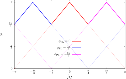
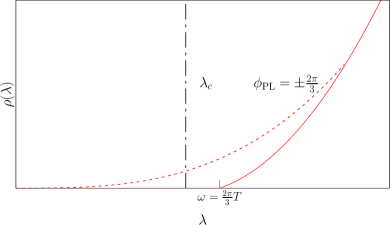
Figure 2: Left: gap function $\omega(\phi_{\textrm{PL}},\hat{\mu}_{I})$ at finite imaginary chemical potential, for $\phi_{\textrm{PL}}$ corresponding to the three centre elements of $\textrm{SU}(3)$. Solid lines indicate the vacuum selected by fermions. Right: sketch of the spectral density at $\hat{\mu}_{I}=\pi$. The solid line is the spectral density in the case of vanishing gauge fields, starting at the gap $\omega=\frac{2\pi}{3}T$, while the dashed line qualitatively shows the spectral density after the inclusion of localised modes penetrating the gap, and $\lambda_{c}$ indicates the position of the mobility edge.

The sea/islands picture discussed in Sec. 3 applies also at finite $\mu_{I}$ after suitably modifying the gap function to $\omega=\omega(\phi_{\textrm{PL}},\hat{\mu}_{I})$. Its behaviour as a function of $\hat{\mu}_{I}$ is shown in Fig. 2 (left) in the case of Polyakov loops ordered along one of the centre elements of $\textrm{SU}(3)$. In the case of $\hat{\mu}_{I}=\pi$ (corresponding to effectively periodic boundary conditions) it reads $\omega(\phi_{\textrm{PL}},\pi)=|\phi_{\textrm{PL}}|T$. This shows that the complex sectors $z=e^{\pm i\frac{2\pi}{3}}$ are equally favoured over the real sector by dynamical fermions, in agreement with the residual $\mathbb{Z}_{2}$ centre symmetry at $\hat{\mu}_{I}=\pi$. Independently of what sector is chosen when the symmetry breaks spontaneously, Polyakov-loop fluctuations to the real sector are favourable localisation centres for the Dirac eigenmodes. In fact, the gap function is locally vanishing there, $\omega(0,\pi)=0$ [see Fig. 2 (left)], and so they can support localised modes with eigenvalues below the gap $\omega(\pm\frac{2\pi}{3},\pi)=\frac{2\pi}{3}T$. The resulting spectral density is sketched in Fig. 2 (right). Moving along the temperature axis at $\hat{\mu}_{I}=\pi$, one then expects localised modes to appear right at $T_{\textrm{RW}}$.

5 Localisation above the Roberge-Weiss temperature

Studying localisation of low Dirac modes along the $\hat{\mu}_{I}=\pi$ line provides the rare opportunity of checking the expectations of the sea/islands picture across a genuine deconfinement phase transition in the presence of dynamical fermions. This was done by us in Ref. Cardinali:2021fpu by means of a numerical study on the lattice. We simulated $N_{f}=2+1$ QCD at physical values of the quark masses using 2-stout improved rooted staggered fermions and a tree-level improved Symanzik gauge action, and studied the statistical properties of the spectrum of the staggered discretisation of the Dirac operator, in order to infer the localisation properties of its eigenmodes. Since the staggered operator is anti-Hermitean, the discussion of Sec. 2 applies without modifications. In particular, we computed $I_{s_{0}}(\lambda)$ along the spectrum and identified the mobility edge $\lambda_{c}$ as the point where it takes its critical value, $I_{s_{0}}(\lambda_{c})=I_{s_{0}}^{\textrm{crit}}$. To check for discretisation effects we used lattices of temporal extension $N_{t}=4,6,8$ in lattice units, and spatial extension $N_{s}$ fixed by setting the aspect ratio to $N_{s}/N_{t}=6$ (as well as 8 for $N_{t}=4$).

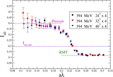
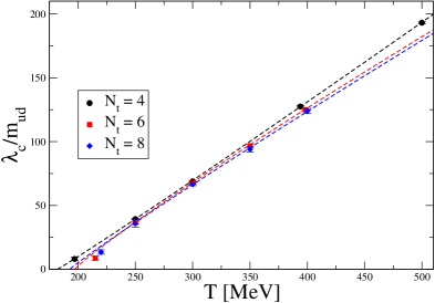
Figure 3: Left: $I_{s_{0}}$ ($s_{0}\simeq 0.508$) in QCD at $\hat{\mu}_{I}=\pi$ and $T=394\leavevmode\nobreak\ \textrm{MeV}$ for $N_{s}^{3}\times N_{t}$ lattices of different spatial size. The Poisson and RMT expectation and the critical value $I_{s_{0}}^{\textrm{crit}}$ Giordano:2013taa are also shown. Right: temperature dependence of the mobility edge in units of $m_{\textrm{ud}}$. Figures from Ref. Cardinali:2021fpu .

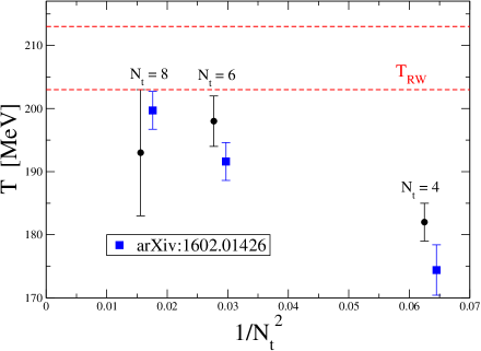
Figure 4: Localisation temperature $T_{\textrm{loc}}(N_{t})$ (black dots) and Roberge-Weiss temperature $T_{\textrm{RW}}(N_{t})$ (blue squares; data from Ref. Bonati:2016pwz ) for the various temporal extensions $N_{t}$. The error band of the continuum extrapolation of $T_{\textrm{RW}}$ is also shown (red dashed lines). Figure from Ref. Cardinali:2021fpu .

An example of our results for $I_{s_{0}}$ is shown in Fig. 3 (left) for $T=394\leavevmode\nobreak\ \textrm{MeV}$. At this temperature we also checked for finite-volume effects, obtaining consistent results for $\lambda_{c}$ for different $N_{s}$. The results for $\lambda_{c}$ in the whole range of temperatures that we investigated is shown in Fig. 3 (right). There we plot the ratio $\lambda_{c}/m_{\textrm{ud}}$, with $m_{\textrm{ud}}$ the mass of the light quarks, against $T=1/(aN_{t})$, for the different choices of $N_{t}$ (and corresponding lattice spacing $a$). The ratio $\lambda_{c}/m_{\textrm{ud}}$ is a renormalisation-group-invariant quantity Kovacs:2012zq ; Giordano:2022ghy , expected to depend mildly on $a$ and to have a finite continuum limit. This is supported by our results.

For each set of data at fixed $N_{t}$ we fitted the temperature dependence of the mobility edge with a power law, $\lambda_{c}/m_{\textrm{ud}}=A(N_{t})[T-T_{\textrm{loc}}(N_{t})]^{B(N_{T})}$, with $T_{\textrm{loc}}(N_{t})$ the localisation temperature where the mobility edge vanishes. Results at the lowest temperature for $N_{t}=6,8$ were excluded from the fits, since they are still affected by large finite-size effects for the available volumes. Results for $T_{\textrm{loc}}(N_{t})$ are shown in Fig. 4, together with the corresponding lattice determinations $T_{\textrm{RW}}(N_{t})$ of the Roberge-Weiss temperature and the resulting continuum extrapolation $T_{\textrm{RW}}$ Bonati:2016pwz . For each $N_{t}$ the results for $T_{\textrm{loc}}(N_{t})$ and $T_{\textrm{RW}}(N_{t})$ are compatible within errors, which strongly supports that the continuum extrapolation $T_{\rm loc}$ of the localisation temperature satisfies $T_{\textrm{loc}}=T_{\textrm{RW}}$.

Our results provide further evidence of the strong connection between deconfinement and the localisation of the low Dirac modes, that happens right at the critical temperature, also in the case of a genuine deconfinement transition in the presence of dynamical fermions.

Acknowledgements MG was partially supported by the NKFIH grant KKP-126769.

References

- (1) T. Banks, A. Casher, Nucl. Phys. B 169, 103 (1980)
- (2) F. Karsch, E. Laermann, C. Schmidt, Phys. Lett. B520, 41 (2001), hep-lat/0107020
- (3) F. Karsch, M. Lütgemeier, Nucl. Phys. B550, 449 (1999), hep-lat/9812023
- (4) A.M. García-García, J.C. Osborn, Phys. Rev. D 75, 034503 (2007), hep-lat/0611019
- (5) T.G. Kovács, F. Pittler, Phys. Rev. D 86, 114515 (2012), 1208.3475
- (6) G. Cossu, S. Hashimoto, J. High Energy Phys. 06, 056 (2016), 1604.00768
- (7) L. Holicki, E.M. Ilgenfritz, L. von Smekal, PoS LATTICE2018, 180 (2018), 1810.01130
- (8) M. Giordano, T.G. Kovács, F. Pittler, Phys. Rev. Lett. 112, 102002 (2014), 1312.1179
- (9) S.M. Nishigaki, M. Giordano, T.G. Kovács, F. Pittler, PoS LATTICE2013, 018 (2014), 1312.3286
- (10) L. Ujfalusi, M. Giordano, F. Pittler, T.G. Kovács, I. Varga, Phys. Rev. D 92, 094513 (2015), 1507.02162
- (11) M. Giordano, T.G. Kovács, Universe 7, 194 (2021), 2104.14388
- (12) F. Bruckmann, T.G. Kovács, S. Schierenberg, Phys. Rev. D 84, 034505 (2011), 1105.5336
- (13) M. Giordano, T.G. Kovács, F. Pittler, J. High Energy Phys. 04, 112 (2015), 1502.02532
- (14) M. Giordano, T.G. Kovács, F. Pittler, J. High Energy Phys. 06, 007 (2016), 1603.09548
- (15) M. Giordano, T.G. Kovács, F. Pittler, Phys. Rev. D 95, 074503 (2017), 1612.05059
- (16) M. Giordano, J. Phys. A 54, 37LT01 (2021), 2009.00486
- (17) M. Giordano (2022), 2206.11109
- (18) M. Giordano, S.D. Katz, T.G. Kovács, F. Pittler, J. High Energy Phys. 02, 055 (2017), 1611.03284
- (19) M. Cardinali, M. D’Elia, F. Garosi, M. Giordano, Phys. Rev. D 105, 014506 (2022), 2110.10029
- (20) P.A. Lee, T.V. Ramakrishnan, Rev. Mod. Phys. 57, 287 (1985)
- (21) B.L. Altshuler, B.I. Shklovskii, Sov. Phys. JETP 64, 127 (1986)
- (22) M.L. Mehta, Random matrices, Vol. 142, 3rd edn. (Elsevier, 2004)
- (23) B.I. Shklovskii, B. Shapiro, B.R. Sears, P. Lambrianides, H.B. Shore, Phys. Rev. B 47, 11487 (1993)
- (24) F. Evers, A.D. Mirlin, Rev. Mod. Phys. 80, 1355 (2008), 0707.4378
- (25) T.G. Kovács, F. Pittler, Phys. Rev. Lett. 105, 192001 (2010), 1006.1205
- (26) T.G. Kovács, R.Á. Vig, Phys. Rev. D 97, 014502 (2018), 1706.03562
- (27) R.Á. Vig, T.G. Kovács, Phys. Rev. D 101, 094511 (2020), 2001.06872
- (28) M. Giordano, J. High Energy Phys. 05, 204 (2019), 1903.04983
- (29) G. Baranka, M. Giordano, Phys. Rev. D 104, 054513 (2021), 2104.03779
- (30) G. Baranka, M. Giordano (2022), 2210.00840
- (31) C. Bonati, M. Cardinali, M. D’Elia, M. Giordano, F. Mazziotti, Phys. Rev. D 103, 034506 (2021), 2012.13246
- (32) A. Roberge, N. Weiss, Nucl. Phys. B 275, 734 (1986)
- (33) C. Bonati, M. D’Elia, M. Mariti, M. Mesiti, F. Negro, F. Sanfilippo, Phys. Rev. D 93, 074504 (2016), 1602.01426
- (34) T.G. Kovács, PoS LATTICE2021, 238 (2022), 2112.05454