Local-to-Global Registration for Bundle-Adjusting Neural Radiance Fields

Abstract

Neural Radiance Fields (NeRF) have achieved photorealistic novel views synthesis; however, the requirement of accurate camera poses limits its application. Despite analysis-by-synthesis extensions for jointly learning neural 3D representations and registering camera frames exist, they are susceptible to suboptimal solutions if poorly initialized. We propose L2G-NeRF, a Local-to-Global registration method for bundle-adjusting Neural Radiance Fields: first, a pixel-wise flexible alignment, followed by a frame-wise constrained parametric alignment. Pixel-wise local alignment is learned in an unsupervised way via a deep network which optimizes photometric reconstruction errors. Frame-wise global alignment is performed using differentiable parameter estimation solvers on the pixel-wise correspondences to find a global transformation. Experiments on synthetic and real-world data show that our method outperforms the current state-of-the-art in terms of high-fidelity reconstruction and resolving large camera pose misalignment. Our module is an easy-to-use plugin that can be applied to NeRF variants and other neural field applications. The Code and supplementary materials are available at https://rover-xingyu.github.io/L2G-NeRF/.

1 Introduction

Recent success with neural fields [47] has caused a resurgence of interest in visual computing problems, where coordinate-based neural networks that represent a field gain traction as a useful parameterization of 2D images [38, 4, 6], and 3D scenes [33, 26, 28]. Commonly, these coordinates are warped to a global coordinate system by camera parameters obtained via computing homography, structure from motion (SfM), or simultaneous localization and mapping (SLAM) [16] with off-the-shelf tools like COLMAP [37], before being fed to the neural fields.

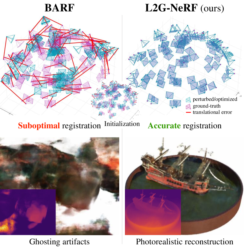
Figure 1: We present L2G-NeRF, a new bundle-adjusting neural radiance fields — employing local-to-global registration — that is much more robust than the current state-of-the-art BARF [23].

This paper considers the generic problem of simultaneously reconstructing the neural fields from RGB images and registering the given camera frames, which is known as a long-standing chicken-and-egg problem — registration is needed to reconstruct the fields, and reconstruction is needed to register the cameras.

One straightforward way to solve this problem is to jointly optimize the camera parameters with the neural fields via backpropagation. Recent work can be broadly placed into two camps: parametric and non-parametric. Parametric methods [23, 43, 19, 9] directly optimize global geometric transformations (e.g. rigid, homography). Non-parametric methods [21, 30] do not make any assumptions on the type of transformation, and attempt to directly optimize some pixel agreement metric (e.g. brightness constancy constraint in optical flow and stereo).

However, both approaches have flaws: parametric methods fail to minimize the photometric errors (falling into the suboptimal solutions) if poorly initialized, as shown in Fig. 1, while non-parametric methods have trouble dealing with large displacements (e.g. although the photometric errors are minimized, the alignments do not obey the geometric constraint). It is natural, therefore, to consider a hybrid approach, combining the benefits of parametric and non-parametric methods together.

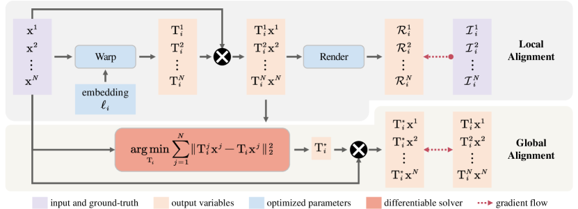
Figure 2: Overall pipeline of proposed framework. Our model has two main branches: 1) Based on query coordinates $\{\mathbf{x}^{j}\}_{j=1}^{N}$ and frame-dependent embeddings $\{\boldsymbol{\ell}_{i}\}_{i=1}^{M}$, a warp neural field $\mathcal{W}$ constructs pixel-wise local transformations $\{\mathbf{T}^{j}_{i}\}_{i=1,j=1}^{M,N}$ and transforms query coordinates into a global coordinate system. Then the color can be rendered via a neural field $\mathcal{R}$ to minimize the photometric error between renderings $\{\mathcal{R}_{i}\}_{i=1}^{M}$ and images $\{\mathcal{I}_{i}\}_{i=1}^{M}$. 2) A differentiable parameter estimation solver produces frame-wise global transformations $\{\mathbf{T}^{\ast}_{i}\}_{i=1}^{M}$ condition on the pixel-wise correspondences. The query coordinates are then transformed to apply a global geometric constraint.

In this paper, we propose L2G-NeRF, a local-to-global process integrating parametric and non-parametric methods for bundle-adjusting neural radiance fields — the joint problem of reconstructing the neural fields and registering the camera parameters, which can be regarded as a type of classic photometric bundle adjustment (BA) [11, 3, 24]. Fig. 2 shows an overview. In the first non-parametric stage, we initialize the alignment by predicting a local transformation field for each pixel of the camera frames. This is achieved by self-supervised training of a deep network to optimize standard photometric reconstruction errors. In the second stage, differentiable parameter estimation solvers are applied to a set of pixel-wise correspondences to obtain a global alignment, which is then used to apply a soft constraint to the local alignment. In summary, we present the following contributions:

• We show that the optimization of bundle-adjusting neural fields is sensitive to initialization, and we present a simple yet effective strategy for local-to-global registration on neural fields.

• We introduce two differentiable parameter estimation solvers for rigid and homography transformation respectively, which play a crucial role in calculating the gradient flow from the global alignment to the local alignment.

• Our method is agnostic to the particular type of neural fields, specifically, we show that the local-to-global process works quite well in 2D neural images and 3D Neural Radiance Fields (NeRF) [28], allowing for applications such as image reconstruction and novel view synthesis.

2 Related Work

SfM and SLAM. SfM [35, 36, 39, 40, 2] and SLAM [31, 15, 29, 48] systems attempt to simultaneously recover the 3D structure and the sensor poses from a set of input images. They reconstruct an explicit geometry (e.g. point clouds) and estimate camera poses through image registration via associating feature correspondences [10, 29] or minimizing photometric errors [3, 14], followed by BA [11, 3, 24].

However, the explicit point clouds assume a diffuse surface, hence cannot model view-dependent appearance. And the sparse nature of point clouds also limits downstream vision tasks, such as photorealistic rendering. In contrast, L2G-NeRF encodes the scenes as coordinate-based neural fields, which is qualified for solving the high-fidelity visual computing problems.

Neural Fields. Recent advances in neural fields [47], which employ coordinate-based neural networks to parameterize physical properties of scenes or objects across space and time, have led to increased interest in solving visual computing problems, causing more accurate, higher fidelity, more expressive, and memory-efficient solutions. They have seen widespread success in problems such as image synthesis [38, 4, 6], 3D shape [33, 26, 8], view-dependent appearance [28, 5, 17, 32], and animation of humans [34, 44, 7].

While these neural fields have achieved impressive results, the requirement of camera parameters limits its application. We are able to get around the requirement with our proposed L2G-NeRF.

Bundle-Adjusting Neural Fields. Since neural fields are end-to-end differentiable, camera parameters can be jointly estimated with the neural fields. The optimization problem is known to be non-convex, and is reflected by NeRF– [43], in which the authors jointly optimize the scene and cameras for forward-facing scenes. Adversarial objective is utilized [25] to relax forward-facing assumption and supports inward-facing $360\degree$ scenes. SCNeRF [19] is further developed to learn the camera intrinsics. BARF [23] shows that bundle-adjusting neural fields could benefit from coarse-to-fine registration. Recent approaches employ Gaussian activations [9] or Sinusoidal activations [46] to overcome local minima in optimization.

Nevertheless, these parametric methods directly optimize global geometric transformations, which are prone to falling into suboptimal solutions if poorly initialized. Non-parametric methods [21, 30] directly optimize decent local transformations based on brightness constancy constraints, whereas they can not handle large displacements. We show that by combining the parametric and non-parametric methods together with a simple local-to-global process, we can achieve surprising anti-noise ability, allowing utilities for various NeRF extensions and other neural field applications.

3 Approach

We first present the formulation of recovering the neural field jointly with camera parameters. Given a collection of images $\{\mathcal{I}_{i}\}_{i=1}^{M}$, we aim to jointly find the parameters $\boldsymbol{\Theta}$ of the neural field $\mathcal{R}$ and the camera parameters (geometric transformation matrices) $\{\mathbf{T}_{i}\}_{i=1}^{M}$ that minimize the photometric error between renderings and images. Let $\{\mathbf{x}^{j}\}_{j=1}^{N}$ be the query coordinates and $\mathcal{I}$ be the imaging function, we formulate the problem as:

$$\min_{\{\mathbf{T}_{i}\}_{i=1}^{M},\boldsymbol{\Theta}}\;\sum_{i=1}^{M}\sum^{N}_{j=1}\big{(}\big{\|}\mathcal{R}(\mathbf{T}_{i}\mathbf{x}^{j};\boldsymbol{\Theta})-\mathcal{I}_{i}(\mathbf{x}^{j})\big{\|}_{2}^{2}\big{)}\;.$$ (1)

Gradient-based optimization is the preferred strategy to solve this nonlinear problem. Nevertheless, gradient-based registration is prone to finding suboptimal poses. Therefore, we propose a simple yet effective strategy for local-to-global registration. The key idea is to apply a pixel-wise flexible alignment that optimizes photometric reconstruction errors individually, followed by a frame-wise alignment to globally constrain the local geometric transformations, which acts like a soft extension of Eq. (1):

$$\min_{\{\mathbf{T}^{j}_{i}\}_{i=1,j=1}^{M,N},\boldsymbol{\Theta}}\;\sum_{i=1}^{M}\sum^{N}_{j=1}\big{(} \big{\|}\mathcal{R}(\mathbf{T}^{j}_{i}\mathbf{x}^{j};\boldsymbol{\Theta})-\mathcal{I}_{i}(\mathbf{x}^{j})\big{\|}_{2}^{2}$$

$$+\lambda \big{\|}\mathbf{T}^{j}_{i}\mathbf{x}^{j}-\mathbf{T}^{\ast}_{i}\mathbf{x}^{j}\big{\|}_{2}^{2}\big{)}\;,$$ (2)

where the pixel-wise local transformations $\{\mathbf{T}^{j}_{i}\}_{i=1,j=1}^{M,N}$ are modeled by a warp neural field $\mathcal{W}$ parametrized by $\boldsymbol{\Phi}$, along with frame-dependent embeddings $\{\boldsymbol{\ell}_{i}\}_{i=1}^{M}$:

$$\mathbf{T}^{j}_{i}=\mathcal{W}(\mathbf{x}^{j};\boldsymbol{\ell}_{i},\boldsymbol{\Phi})\;,$$ (3)

and the frame-wise global transformations $\{\mathbf{T}^{\ast}_{i}\}_{i=1}^{M}$ are solved by using differentiable parameter estimation solvers on the pixel-wise correspondences:

$$\mathbf{T}^{\ast}_{i}=\operatorname*{arg\,min}_{\mathbf{T}_{i}} \sum^{N}_{j=1}\big{\|}\mathbf{T}^{j}_{i}\mathbf{x}^{j}-\mathbf{T}_{i}\mathbf{x}^{j}\big{\|}_{2}^{2}.$$ (4)

3.1 Neural Image Alignment (2D)

To develop intuition, we first consider the case of a 2D neural image alignment problem. More specifically, let $\mathbf{x}\in\mathbb{R}^{2}$ be the 2D pixel coordinates and $\mathcal{I}:\mathbb{R}^{2}\to\mathbb{R}^{3}$, we aim to optimize a 2D neural field parameterized as the weights $\boldsymbol{\Theta}$ of a multilayer perceptron (MLP) $f_{{\mathcal{R}}}:\mathbb{R}^{2}\to\mathbb{R}^{3}$:

$$\mathcal{R}(\mathbf{T}\mathbf{x};\boldsymbol{\Theta})=f_{{\mathcal{R}}}(\mathbf{T}\mathbf{x};\boldsymbol{\Theta})\;,$$ (5)

while also solving for geometric transformation parameters as $\mathbf{T}=[\mathbf{R}|\mathbf{t}]\in\mathrm{SE}(2)$ or $\mathbf{T}\in\mathrm{SL}(3)$, where $\mathbf{R}\in\mathrm{SO}(2)$ and $\mathbf{t}\in\mathbb{R}^{2}$ denote the rigid rotation and translation, and $\mathbf{T}\in\mathrm{SL}(3)$ denotes the homography transformation matrix, respectively. We use another MLP with weights $\boldsymbol{\Phi}$ to model the coordinate-based warp neural field $f_{{\mathcal{W}}}:\mathbb{R}^{2}\to\mathbb{R}^{3}$ condition on the frame-dependent embedding $\boldsymbol{\ell}$:

$$\mathcal{W}(\mathbf{x};\boldsymbol{\ell},\boldsymbol{\Phi})=\exp\big{(}f_{{\mathcal{W}}}(\mathbf{x};\boldsymbol{\ell},\boldsymbol{\Phi})\big{)}\;,$$ (6)

where the operator $\exp(\cdot)$ denotes the exponential map from Lie algebra $\mathfrak{se}(2)$ or $\mathfrak{sl}(3)$ to the Lie group $\mathrm{SE}(2)$ or $\mathrm{SL}(3)$, which ensures that the optimized transformation matrices $\mathbf{T}$ lie on the Lie group manifold during the gradient-based optimization.

3.2 Bundle-Adjusting Neural Radiance Fields (3D)

We then discuss the problem of simultaneously recovering the 3D Neural Radiance Fields (NeRF) [28] and the camera poses. Given an 3D point, we predict the RGB color $\mathbf{c}\in\mathbb{R}^{3}$ and volume density $\sigma\in\mathbb{R}$ via an MLP $f_{{\mathcal{R}}}:\mathbb{R}^{3}\to\mathbb{R}^{4}$, which encodes the 3D scene using network parameters. We begin by formulating NeRF’s rendering process in the space of the camera view. Denoting the homogeneous coordinates of pixel coordinates $\mathbf{u}\in\mathbb{R}^{2}$ as $\mathbf{x}=[\mathbf{u};1]^{\top}\in\mathbb{R}^{3}$, the 3D point along the viewing ray at depth $z_{i}$ can be expressed as $z_{i}\mathbf{x}$, thus the query quantity $\mathbf{y}=[\mathbf{c};\sigma]^{\top}=f_{{\mathcal{R}}}(z_{i}\mathbf{x};\boldsymbol{\Theta})$, where $\boldsymbol{\Theta}$ is the parameters of $f_{{\mathcal{R}}}$. Then the rendering color $\mathcal{R}$ at pixel location $\mathbf{x}$ can be composed by volume rendering

$$\mathcal{R}(\mathbf{x})=\int_{z_{\text{near}}}^{z_{\text{far}}}T(\mathbf{x},z)\sigma(z\mathbf{x})\mathbf{c}(z\mathbf{x})\mathrm{d}z\;,$$ (7)

where $T(\mathbf{x},z)=\exp\!\big{(}\!-\!\int_{z_{\text{near}}}^{z}\sigma(z^{\prime}\mathbf{x})\mathrm{d}z^{\prime}\big{)}$, and $z_{\text{near}}$ and $z_{\text{far}}$ are the near and far depth bounds of the scene. Numerically, the integral formulation is discretely approximated using $K$ points sampled along a ray at depth $\{z_{1},\dots,z_{K}\}$. The network $f_{{\mathcal{R}}}$ is evaluated $K$ times, and the outputs $\{\mathbf{y}_{1},\dots,\mathbf{y}_{K}\}$ are then composited via volume rendering. Denoting the differentiable and deterministic compositing function as $g:\mathbb{R}^{4K}\to\mathbb{R}^{3}$, such that $\mathcal{R}(\mathbf{x})$ can be expressed as $\mathcal{R}(\mathbf{x})=g\left(\mathbf{y}_{1},\dots,\mathbf{y}_{K}\right)$.

Here the camera poses are parametrized by $\mathbf{T}=[\mathbf{R}|\mathbf{t}]\in\mathrm{SE}(3)$, where $\mathbf{R}\in\mathrm{SO}(3)$ and $\mathbf{t}\in\mathbb{R}^{3}$. Next, we use a 3D rigid transformation $\mathbf{T}$ to transform the 3D point $z_{i}\mathbf{x}$ from camera view space to world coordinates, and formulate the rendering color at pixel $\mathbf{x}$ as

$$\mathcal{R}(\mathbf{T}\mathbf{x};\boldsymbol{\Theta})=g\Big{(}f_{{\mathcal{R}}}(\mathbf{T}z_{1}\mathbf{x};\boldsymbol{\Theta}),\dots,f_{{\mathcal{R}}}(\mathbf{T}z_{K}\mathbf{x};\boldsymbol{\Theta})\Big{)}.$$ (8)

Similar to neural image alignment, We use another MLP with weights $\boldsymbol{\Phi}$ to model the coordinate-based warp neural field $f_{{\mathcal{W}}}:\mathbb{R}^{2}\to\mathbb{R}^{6}$ condition on the frame-dependent embedding $\boldsymbol{\ell}$:

$$\mathcal{W}(\mathbf{x};\boldsymbol{\ell},\boldsymbol{\Phi})=\exp\big{(}f_{{\mathcal{W}}}(\mathbf{x};\boldsymbol{\ell},\boldsymbol{\Phi})\big{)}\;,$$ (9)

where the operator $\exp(\cdot)$ denotes the exponential map from Lie algebra $\mathfrak{se}(3)$ to the Lie group $\mathrm{SE}(3)$.

3.3 Differentiable Parameter Estimation

The local-to-global process allows L2G-NeRF to discover the correct registration with an initially flexible pixel-wise alignment and later shift focus to constrained parametric alignment. We derive the gradient flow of global alignment objective $\mathcal{L}^{j}_{i}=\big{\|}\mathbf{T}^{j}_{i}\mathbf{x}^{j}-\mathbf{T}^{\ast}_{i}\mathbf{x}^{j}\big{\|}_{2}^{2}$ w.r.t. the parameters $\boldsymbol{\Phi}$ of warp neural field $\mathcal{W}$ as

$$\small\frac{\partial\mathcal{L}^{j}_{i}}{\partial\boldsymbol{\Phi}}=\frac{\partial\mathcal{L}^{j}_{i}}{\partial\mathbf{T}^{j}_{i}}\frac{\partial\mathbf{T}^{j}_{i}}{\partial\boldsymbol{\Phi}}+\frac{\partial\mathcal{L}^{j}_{i}}{\partial\mathbf{T}^{\ast}_{i}}\sum^{N}_{j=1}\frac{\partial\mathbf{T}^{\ast}_{i}}{\partial\mathbf{T}^{j}_{i}}\frac{\partial\mathbf{T}^{j}_{i}}{\partial\boldsymbol{\Phi}}\;.$$ (10)

Such that a differentiable solver is of critical importance to calculating the gradient of $\mathbf{T}^{\ast}_{i}$ w.r.t. $\mathbf{T}^{j}_{i}$ then backpropagated to update the parameters $\boldsymbol{\Phi}$. Next, we elaborate two differentiable solvers for rigid and homography transformation, respectively.

Rigid parametric alignment. In the rigid parametric alignment problem, we assume $\{\mathbf{T}^{j}\mathbf{x}^{j}\}_{j=1}^{N}$ is transformed from $\{\mathbf{x}^{j}\}_{j=1}^{N}$ by an unknown global rigid transformation $\mathbf{T}=[\mathbf{R}|\mathbf{t}]\in\mathrm{SE}(2)$ or $\mathbf{T}=[\mathbf{R}|\mathbf{t}]\in\mathrm{SE}(3)$. To solve this classic orthogonal Procrustes problem [18], we define centroids of $\{\mathbf{x}^{j}\}_{j=1}^{N}$ and $\{\mathbf{T}^{j}\mathbf{x}^{j}\}_{j=1}^{N}$ as

$$\overline{\mathbf{x}}=\frac{1}{N}\sum^{N}_{j=1}(\mathbf{x}^{j})\quad\textrm{and}\quad\overline{\mathbf{T}\mathbf{x}}=\frac{1}{N}\sum^{N}_{j=1}(\mathbf{T}^{j}\mathbf{x}^{j}).$$ (11)

Then the cross-covariance matrix $\boldsymbol{H}$ is given by

$$\boldsymbol{H}=\sum_{j=1}^{N}(\mathbf{x}^{j}-\overline{\mathbf{x}})(\mathbf{T}^{j}\mathbf{x}^{j}-\overline{\mathbf{T}\mathbf{x}})^{\top}.$$ (12)

We use Singular Value Decomposition (SVD) to decompose $\boldsymbol{H}$ as introduced in [41, 20]:

$$\boldsymbol{H}=\boldsymbol{U}\boldsymbol{S}\boldsymbol{V}^{\top}.$$ (13)

Thus the optimal transformation minimizing Eq. (4) is given in closed form by

$$\mathbf{R}=\boldsymbol{V}\boldsymbol{U}^{\top}\quad\textrm{and}\quad\mathbf{t}=-\mathbf{R}\overline{\mathbf{x}}+\overline{\mathbf{T}\mathbf{x}}.$$ (14)

Homography parametric alignment. In the homography parametric alignment problem, we assume $\{{\mathbf{x}^{j}}^{\prime}=\mathbf{T}^{j}\mathbf{x}^{j}\}_{j=1}^{N}$ is transformed from $\{\mathbf{x}^{j}\}_{j=1}^{N}$ by an unknown homography transformation $\mathbf{T}\in\mathrm{SL}(3)$. Written element by element, in homogenous coordinates, we get the following constraint:

$$\left[\begin{array}[]{c}{\mathbf{x}^{j}}^{\prime}_{1}\\ {\mathbf{x}^{j}}^{\prime}_{2}\\ 1\end{array}\right]=\left[\begin{array}[]{lll}\mathbf{T}_{11}&\mathbf{T}_{12}&\mathbf{T}_{13}\\ \mathbf{T}_{21}&\mathbf{T}_{22}&\mathbf{T}_{23}\\ \mathbf{T}_{31}&\mathbf{T}_{32}&\mathbf{T}_{33}\end{array}\right]\left[\begin{array}[]{c}{\mathbf{x}^{j}}_{1}\\ {\mathbf{x}^{j}}_{2}\\ 1\end{array}\right].$$ (24)

Rearranging Eq. (24) as [1], we get $\mathbf{A}^{j}\mathbf{h}=\mathbf{0}$, where

$$\small\begin{aligned} \mathbf{A}^{j}&=\left[\begin{array}[]{ccccccccc}0&0&0&-{\mathbf{x}^{j}}_{1}&-{\mathbf{x}^{j}}_{2}&-1&{\mathbf{x}^{j}}^{\prime}_{2}{\mathbf{x}^{j}}_{1}&{\mathbf{x}^{j}}^{\prime}_{2}{\mathbf{x}^{j}}_{2}&{\mathbf{x}^{j}}^{\prime}_{2}\\ {\mathbf{x}^{j}}_{1}&{\mathbf{x}^{j}}_{2}&1&0&0&0&-{\mathbf{x}^{j}}^{\prime}_{1}{\mathbf{x}^{j}}_{1}&-{\mathbf{x}^{j}}^{\prime}_{1}{\mathbf{x}^{j}}_{2}&-{\mathbf{x}^{j}}^{\prime}_{1}\end{array}\right]\\ \mathbf{h}&=\left(\mathbf{T}_{11},\mathbf{T}_{12},\mathbf{T}_{13},\mathbf{T}_{21},\mathbf{T}_{22},\mathbf{T}_{23},\mathbf{T}_{31},\mathbf{T}_{32},\mathbf{T}_{33}\right)^{\top}\end{aligned}$$ (25)

Given the set of correspondences, we can form the linear system of equations $\boldsymbol{A}\mathbf{h}=\mathbf{0}$, where $\boldsymbol{A}=(\mathbf{A}^{1}\dots\mathbf{A}^{N})^{\top}$. Thus we can solve the Homogeneous Linear Least Squares problem and calculate the non-trivial solution by SVD decomposition:

$$\small\boldsymbol{A}=\boldsymbol{U}\boldsymbol{S}\boldsymbol{V}^{\top}=\sum_{l=1}^{9}\sigma_{l}\boldsymbol{u}_{l}\boldsymbol{v}_{l}^{\top},$$ (26)

where singular value $\sigma_{l}$ represents the reprojection error. Then we take the singular vector $\boldsymbol{v}_{9}$ that corresponds to the smallest singular value $\sigma_{9}$ as the solution of $\mathbf{h}$, and reshape it into the homography transformation matrix $\mathbf{T}$.

Figure 3: Color-coded patch reconstructions of neural image alignment under rigid perturbations. The optimized warps are shown in Fig. 5 with corresponding colors. L2G-NeRF is able to recover accurate alignment and photorealistic image reconstruction with local-to-global registration, while baselines result in suboptimal alignment.

Figure 4: Color-coded patch reconstructions of neural image alignment under homography perturbations.

Figure 5: Qualitative results of neural image alignment experiment under rigid perturbations. Given color-coded patches (Fig. 3), we recover the alignment (top row) and the neural field of the entire image (bottom row).

Method	Rigid perturbations		Homography perturbations
	Corner error (pixels) $\downarrow$	Patch PSNR $\uparrow$	Corner error (pixels) $\downarrow$	Patch PSNR $\uparrow$
Naïve	120.00	14.83	55.80	21.79
BARF [23]	110.20	17.78	30.21	23.24
Ours	0.31	29.25	0.76	31.93

Table 1: Quantitative results of neural image alignment experiment under rigid and homography perturbations. L2G-NeRF optimizes for high-quality alignment and patch reconstruction, while baselines exhibit large errors.

Figure 6: Qualitative results of neural image alignment experiment under homography perturbations.

4 Experiments

We first unfold the validation of L2G-NeRF and baselines on a 2D neural image alignment experiment, and then show that the local-to-global registration strategy can also be generalized to learn 3D neural fields (NeRF [28]) from both synthetic data and photo collections.

4.1 Neural image Alignment (2D)

We choose two representative images of “Girl With a Pearl Earring” renovation ©Koorosh Orooj (CC BY-SA 4.0) and “cat” from ImageNet [12] for rigid and homography image alignment experiments, respectively. As shown in Fig. 3 and Fig. 4, given $M=5$ patches sampled from the original image with rigid or homography perturbations, we optimize Eq. (3) to find the rigid transformation $\mathbf{T}\in\mathrm{SE}(2)$ or homography transformation $\mathbf{T}\in\mathrm{SL}(3)$ for each patch with network $f_{{\mathcal{W}}}$, and learn the neural field of the entire image (Fig. 5 and Fig. 6) with network $f_{{\mathcal{R}}}$ at the same time. We follow [23] to initialize patch warps as identity and anchor the first warp to align the neural image to the raw image.

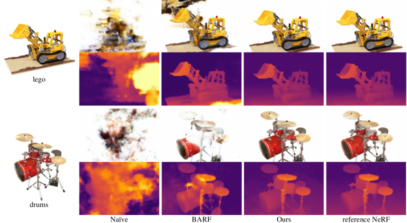
Figure 7: Qualitative results of bundle-adjusting neural radiance fields on synthetic scenes. The image synthesis and the expected depth are visualized with ray compositing in the top and bottom rows, respectively. While baselines render artifacts due to less-than-optimal registration, L2G-NeRF achieves qualified visual quality, which is comparable to the reference NeRF trained under ground-truth poses.

Experimental settings. We evaluate our proposed method against a bundle-adjusting extension of the naïve 2D neural field, dubbed as Naïve, and the current state-of-the-art BARF [23], which employs a coarse-to-fine strategy for registration. We use the default coarse-to-fine scheduling, architecture and training procedure of neural field $f_{{\mathcal{R}}}$ for both BARF and L2G-NeRF. For L2G-NeRF, We use a ReLU MLP for $f_{{\mathcal{W}}}$ with six 256-dimensional hidden units, and use the embedding with 128 dimensions for each image to model the frame-dependent embeddings $\{\boldsymbol{\ell}_{i}\}_{i=1}^{M}$. We set multiplier $\lambda$ of the global alignment objective to $1\times 10^{2}$.

Results. We visualize the rigid and homography registration results in Fig. 5 and Fig. 6. Alignment with Naïve results in ghosting artifacts in the recovered neural image due to large misalignment. On the other hand, alignment with BARF improves registration results but still falls into the suboptimal solutions, and struggles with image reconstruction. As L2G-NeRF discovers the precise geometric warps of all patches, it can optimize the neural image with high fidelity. We report the quantitative results in Table 1, where we use the mean average corner error (L2 distance between the ground truth corner position and the estimated corner position) [13, 22] and PSNR as the evaluation criteria for registration and reconstruction, respectively. The experiment of image alignment shows how local-to-global strategy has a wide range of benefits for both rigid and homography registration for 2D neural fields, which can be easily extended to other geometric transformations.

Scene	Camera pose registration						View synthesis quality
	Rotation ($\degree$) $\downarrow$			Translation $\downarrow$			PSNR $\uparrow$				SSIM $\uparrow$				LPIPS $\downarrow$
	Naïve	BARF	Ours	Naïve	BARF	Ours	Naïve	BARF	Ours	ref.	Naïve	BARF	Ours	ref.	Naïve	BARF	Ours	ref.
										NeRF				NeRF				NeRF
Chair	1.39	2.58	0.14	60.32	10.43	0.28	14.13	27.84	30.99	31.93	0.83	0.92	0.95	0.96	0.39	0.06	0.05	0.04
Drums	7.99	4.54	0.06	78.20	19.19	0.40	11.63	21.92	23.75	23.98	0.61	0.87	0.90	0.90	0.62	0.14	0.10	0.10
Ficus	3.13	1.65	0.26	48.78	5.46	1.11	14.30	25.85	26.11	26.66	0.83	0.93	0.93	0.94	0.33	0.07	0.06	0.05
Hotdog	7.04	2.42	0.27	58.37	14.98	1.42	15.10	27.34	34.56	34.90	0.74	0.93	0.97	0.97	0.42	0.06	0.03	0.03
Lego	7.82	9.93	0.09	81.93	47.42	0.37	11.36	14.48	27.71	29.29	0.61	0.69	0.91	0.94	0.56	0.29	0.06	0.04
Materials	5.57	0.68	0.06	47.56	4.97	0.28	11.51	26.29	27.60	28.54	0.64	0.92	0.93	0.94	0.49	0.08	0.06	0.05
Mic	4.43	10.44	0.10	77.47	45.66	0.44	13.14	12.20	30.91	31.96	0.85	0.76	0.97	0.97	0.43	0.41	0.05	0.04
Ship	11.10	23.90	0.19	112.01	90.62	0.61	9.41	8.19	27.31	28.06	0.50	0.50	0.85	0.86	0.64	0.63	0.13	0.12
Mean	6.06	7.02	0.15	70.58	29.84	0.61	12.57	20.51	28.62	29.42	0.70	0.82	0.93	0.94	0.49	0.22	0.07	0.06

Table 2: Quantitative results of bundle-adjusting neural radiance fields on synthetic scenes. L2G-NeRF successfully optimizes camera poses, thus rendering high-quality images comparable to the reference NeRF model (trained using ground-truth camera poses), outperforming the baselines on all evaluation criteria. Translation errors are scaled by $100$.

4.2 NeRF (3D): Synthetic Objects

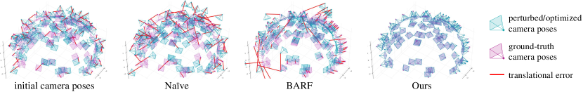
Figure 8: Visual comparison of the initial and optimized camera poses (Procrustes aligned) for the lego scene. L2G-NeRF properly aligns all of the camera frames while baselines get stuck at suboptimal poses.

This section investigates the challenge of learning 3D Neural Radiance Fields (NeRF) [28] from noisy camera poses. We evaluate L2G-NeRF and baselines on 8 synthetic object-centric scenes [28], in which each scene has $M=100$ rendered images with ground-truth camera poses for training.

Experimental settings. For each scene, we synthetically perturb the camera poses $\mathbf{T}\in\mathrm{SE}(3)$ with additive noise $\xi\in\mathfrak{se}(3)$ and $\xi\sim\mathcal{N}(\mathbf{0},n\mathbf{I})$ as initial poses, where the multiplier $n$ is scene-dependent and given in the supplementary materials. We assume known camera intrinsics and minimize the objective in Eq. (3) for optimizing the 3D neural fields $f_{{\mathcal{R}}}$ and the warp field $f_{{\mathcal{W}}}$ that finds rigid transformations relative to the initial poses. We evaluate L2G-NeRF against a naïve extension of the original NeRF model that jointly optimizes poses, dubbed as Naïve, and the coarse-to-fine bundle-adjusting neural radiance fields (BARF) [23].

Implementation details. Our implementation of NeRF and BARF follows[23]. For L2G-NeRF, We use a 6-layer ReLU MLP for $f_{{\mathcal{W}}}$ with 256-dimensional hidden units. We set multiplier $\lambda$ of the global alignment objective to $1\times 10^{2}$ and employ the Adam optimizer to train all models for $200$K iterations with a learning rate that begins at $5\!\times\!10^{-4}$ for the 3D neural field $f_{{\mathcal{R}}}$, and $1\!\times\!10^{-3}$ for the warp field $f_{{\mathcal{W}}}$, and exponentially decays to $1\!\times\!10^{-4}$ and $1\!\times\!10^{-8}$, respectively. We follow the default coarse-to-fine scheduling for both BARF and L2G-NeRF.

Evaluation criteria. Following BARF [23], we use Procrustes analysis to find a 3D similarity transformation that aligns the optimized poses to the ground truth before evaluating registration quality (quantitative results based on average translation and rotation errors), and perform test-time photometric pose optimization [24, 49, 23] before evaluating view synthesis quality (quantitative results based on PSNR, SSIM and LPIPS [50]).

Results. We visualize the results in Fig. 7, which are quantitatively reflected in Table 2. On both sides of reconstruction and registration, L2G-NeRF achieves the best performance. Fig. 8 shows that L2G-NeRF can achieve near-perfect registration for the synthetic scenes. Naïve NeRF suffers from suboptimal registration and ghosting artifacts. BARF is able to recover a part of the pose misalignment and produce plausible reconstructions. However, it still suffers from blur artifacts like the fog effect around the objects. This fog effect is the consequence of BARF’s attempt to reconstruct the scenes with half-baked registration. We then compare the rendering quality to the reference standard NeRF (ref. NeRF), which is trained using ground truth poses, demonstrating that L2G-NeRF can achieve comparable image quality, despite being initialized from a significant camera pose misalignment.

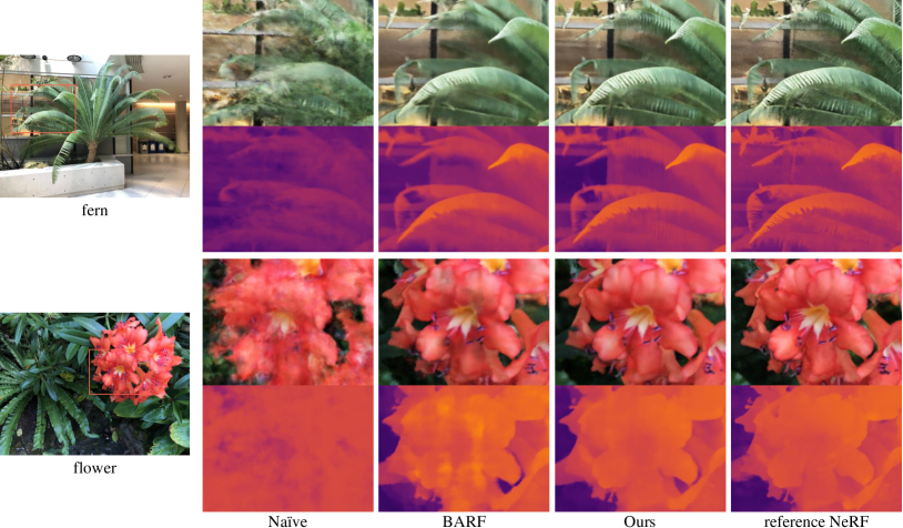
Figure 9: Qualitative results of bundle-adjusting neural radiance fields on real-world scenes. While BARF and L2G-NeRF can jointly optimize poses and scenes, L2G-NeRF produces higher fidelity results, which is competitive to reference NeRF trained under SfM poses.

Scene	Camera pose registration						View synthesis quality
	Rotation ($\degree$) $\downarrow$			Translation $\downarrow$			PSNR $\uparrow$				SSIM $\uparrow$				LPIPS $\downarrow$
	Naïve	BARF	Ours	Naïve	BARF	Ours	Naïve	BARF	Ours	ref.	Naïve	BARF	Ours	ref.	Naïve	BARF	Ours	ref.
										NeRF				NeRF				NeRF
Fern	8.05	0.17	0.20	1.74	0.19	0.18	16.28	23.88	24.57	24.19	0.39	0.71	0.75	0.74	0.54	0.31	0.26	0.25
Flower	22.41	0.31	0.33	5.81	0.22	0.24	12.28	24.29	24.90	22.97	0.21	0.71	0.74	0.66	0.66	0.20	0.17	0.26
Fortress	171.77	0.41	0.25	47.90	0.33	0.25	11.56	29.06	29.27	26.12	0.29	0.82	0.84	0.79	0.83	0.13	0.11	0.19
Horns	29.42	0.11	0.22	12.83	0.16	0.27	8.94	23.29	23.12	20.45	0.22	0.74	0.74	0.63	0.82	0.29	0.26	0.41
Leaves	79.47	1.13	0.79	12.42	0.24	0.34	9.10	18.91	19.02	13.71	0.06	0.55	0.56	0.21	0.80	0.35	0.33	0.58
Orchids	41.75	0.60	0.67	19.99	0.39	0.41	9.93	19.46	19.71	17.26	0.09	0.57	0.61	0.51	0.81	0.29	0.25	0.31
Room	175.06	0.31	0.30	65.48	0.28	0.23	11.48	32.05	32.25	32.94	0.31	0.94	0.95	0.95	0.85	0.10	0.08	0.07
T-rex	166.21	1.38	0.89	55.02	0.86	0.64	9.17	22.92	23.49	21.86	0.16	0.78	0.80	0.74	0.86	0.20	0.16	0.25
Mean	86.77	0.55	0.46	27.65	0.33	0.32	11.09	24.23	24.54	22.44	0.22	0.73	0.75	0.65	0.77	0.23	0.20	0.29

Table 3: Quantitative results of bundle-adjusting neural radiance fields on real-world scenes. L2G-NeRF outperforms baselines and achieves high-quality view synthesis that is competitive to reference NeRF trained under SfM poses. Translation errors are scaled by $100$.

4.3 NeRF (3D): Real-World Scenes

We further explore the challenge of employing NeRF to learn 3D neural fields in real-world scenes with unknown camera poses. We evaluate our method and baselines on the standard benchmark LLFF dataset [27], which is captured by hand-held cameras that record 8 forward-facing scenes in the real world.

Experimental settings. We initialize all cameras with the identity transformation, i.e. $\mathbf{T}_{i}=\mathbf{I}\;\;\forall i$, and use the camera intrinsics provided by LLFF dataset. We compare against the Naïve extension of NeRF [28], BARF [23], and use the same evaluation metrics as described in the experiments of synthetic objects (Sec. 4.2).

Implementation details. We follow the same architectural settings and coarse-to-fine scheduling from the BARF [23]. For simplicity, We train without additional hierarchical sampling. We train all models for $200$K iterations with a learning rate of $1\!\times\!10^{-3}$ for the 3D neural field $f_{{\mathcal{R}}}$ decaying to $1\!\times\!10^{-4}$, and $3\!\times\!10^{-3}$ for the warp field $f_{{\mathcal{W}}}$ decaying to $1\!\times\!10^{-8}$. We use the same architecture of the warp field for L2G-NeRF described in Sec. 4.2.

Results. Quantitative results are summarized in Table 3. Naïve NeRF diverges to wrong camera poses, producing poor view synthesis that cannot compete with BARF. In contrast, L2G-NeRF achieves competitive registration errors compared to BARF while outperforming the others on all view synthesis criteria. Actually, we note that the camera poses provided in LLFF are also estimations from SfM packages [37]; therefore, the pose evaluation is a noisy indication. Based on the fact that more accurate registration yields more photorealistic view synthesis, we recommend using view synthesis quality as the primary criterion for real-world scenes. The high-fidelity visual quality shown in Fig. 9 highlights the ability of L2G-NeRF to register cameras and reconstruct neural fields from scratch.

5 Conclusion

We present Local-to-Global Registration for Bundle-Adjusting Neural Radiance Fields (L2G-NeRF), which is demonstrated by extensive experiments that can effectively learn the neural fields of scenes and resolve large camera pose misalignment at the same time. By establishing a unified formulation of bundle-adjusting neural fields, we demonstrate that local-to-global registration is beneficial for both 2D and 3D neural fields, allowing for various applications of diverse neural fields. Code and models will be made available to the research community to facilitate reproducible research.

Although local-to-global registration is much more robust than current state-of-the-art [23], L2G-NeRF still can not recover camera poses from scratch (identity transformation) for inward-facing $360\degree$ scenes, where large displacements of rotation exist. Specific methods such as epipolar geometry and graph optimization could be employed to handle these issues.

Here we provide more implementation details and experimental results. We encourage readers to view the supplementary video for an intuitive experience about different types of bundle-adjusting neural radiance fields.

A Additional Details

A.1 Time Consumption

We implement all experiments on a single NVIDIA GeForce RTX 2080 Ti GPU. As shown in Table 4, L2G-NeRF takes about 4.5 and 8 hours for training in synthetic objects and real-world scenes, respectively, while training BARF [23] takes about 8 and 10.5 hours. As a reference, we also compare time consumption against the ref. NeRF [28] trained under ground-truth poses (without the requirement of optimizing poses), showing that L2G-NeRF can achieve comparable time consumption. The time analysis indicates that calculating the gradient w.r.t. local pose (local-to-global registration) is more efficient than calculating the gradient w.r.t. global pose (global registration).

Scene	BARF	Ours	ref. NeRF
Synthetic objects	08:18	04:35	04:30
Real-World scenes	10:38	07:42	07:25

Table 4: Average training time (hh:mm).

Scene	Chair	Drums	Ficus	Hotdog	Lego	Materials	Mic	Ship
$n_{r}$	0.01	0.05	0.03	0.04	0.07	0.04	0.04	0.09
$n_{t}$	0.4	0.5	0.3	0.4	0.5	0.3	0.5	0.7

Table 5: Multiplier of pose perturbation for synthetic scenes.

Scene	Fern	Flower	Fortress	Horns	Leaves	Orchids	Room	T-rex
$\lambda$	$1\times 10^{2}$	$1\times 10^{3}$	$1\times 10^{5}$	$1\times 10^{5}$	$1\times 10^{2}$	$1\times 10^{2}$	$1\times 10^{5}$	$1\times 10^{5}$

Table 6: Multiplier $\lambda$ of global alignment objective.

A.2 Camera Pose Perturbation

In all experiments, we always use the same initial conditions for all methods (fixed random seeds). For each object of synthetic scenes, we perturb the camera poses with additive noise as initial poses. Note that the way we add noise differs from  [23], which perturbs ground-truth camera poses using left multiplication (transform cameras around the object’s center). Transformed cameras almost still face the object’s center, and the distances between the cameras and the object are almost unchanged. In contrast, we perturb ground-truth camera poses using right multiplication (transform cameras around themselves), thereby perturbing camera viewing directions (not always toward the object’s center) and camera positions (including the distances from them to the object), respectively.

The 6-DoF perturbation is parametrized by $\mathbf{T}=[\mathbf{R}|\mathbf{t}]\in\mathrm{SE}(3)$, where $\mathbf{R}\in\mathrm{SO}(3)$, $\mathbf{t}\in\mathbb{R}^{3}$, and $\mathbf{R}$ is generated by exponential map $\exp\big{(}\mathbf{r}\big{)}$ from the Lie algebra $\mathfrak{so}(3)$ to the Lie group $\mathrm{SO}(3)$. The additive rotation noise $\mathbf{r}\in\mathfrak{so}(3)$ and translation noise $\mathbf{t}\in\mathbb{R}^{3}$ are distributed as $\mathbf{r}\sim\mathcal{N}(\mathbf{0},n_{r}\mathbf{I})$ and $\mathbf{t}\sim\mathcal{N}(\mathbf{0},n_{t}\mathbf{I})$, where the multiplier $n_{r}$ and $n_{t}$ are scene-dependent and given in Table 5.

Scene	Camera pose registration								View synthesis quality
	Rotation ($\degree$) $\downarrow$				Translation $\downarrow$				PSNR $\uparrow$				LPIPS $\downarrow$
	$1\times 10^{2}$	$1\times 10^{3}$	$1\times 10^{4}$	$1\times 10^{5}$	$1\times 10^{2}$	$1\times 10^{3}$	$1\times 10^{4}$	$1\times 10^{5}$	$1\times 10^{2}$	$1\times 10^{3}$	$1\times 10^{4}$	$1\times 10^{5}$	$1\times 10^{2}$	$1\times 10^{3}$	$1\times 10^{4}$	$1\times 10^{5}$
Flower	0.44	0.33	\	\	0.30	0.24	\	\	24.59	24.90	\	\	0.18	0.17	\	\
Horns	0.36	0.24	0.23	0.22	0.80	0.57	0.32	0.27	22.51	22.84	22.82	23.12	0.28	0.28	0.27	0.26

Table 7: Ablation on the global alignment objective multiplier $\lambda$.

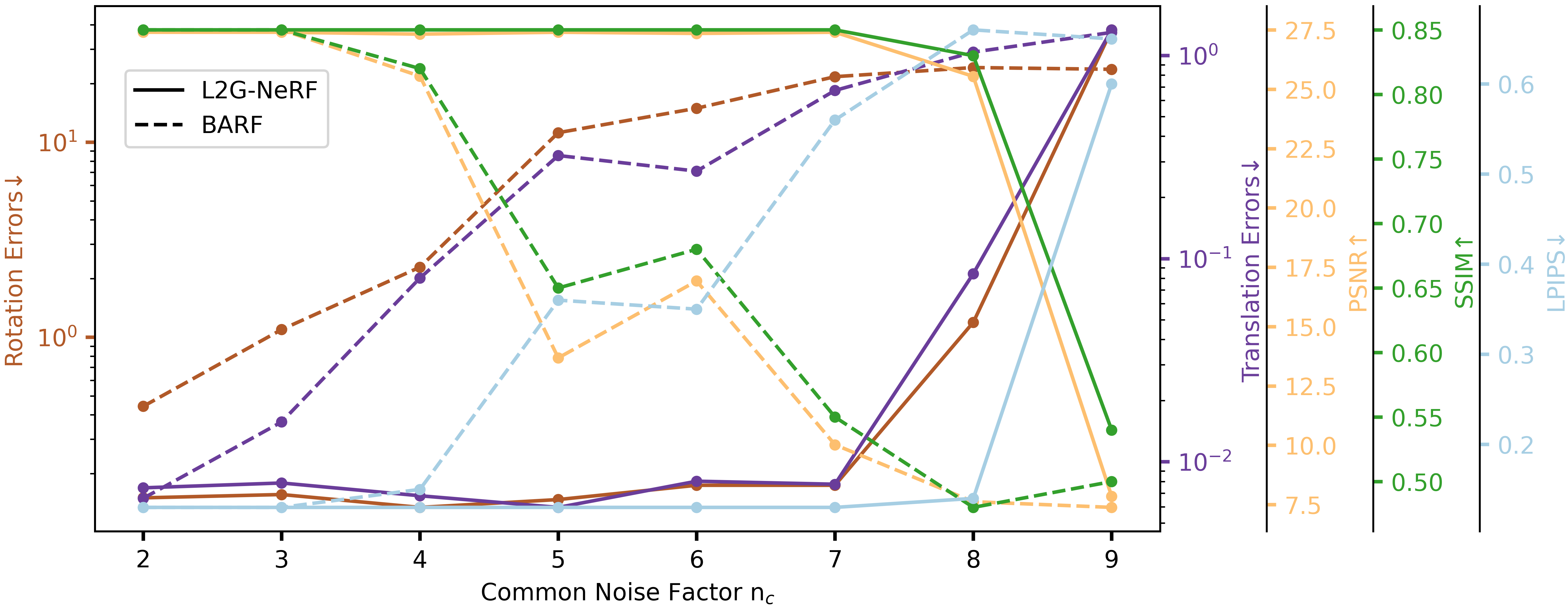
Figure 10: Convergence w.r.t. camera pose perturbation.

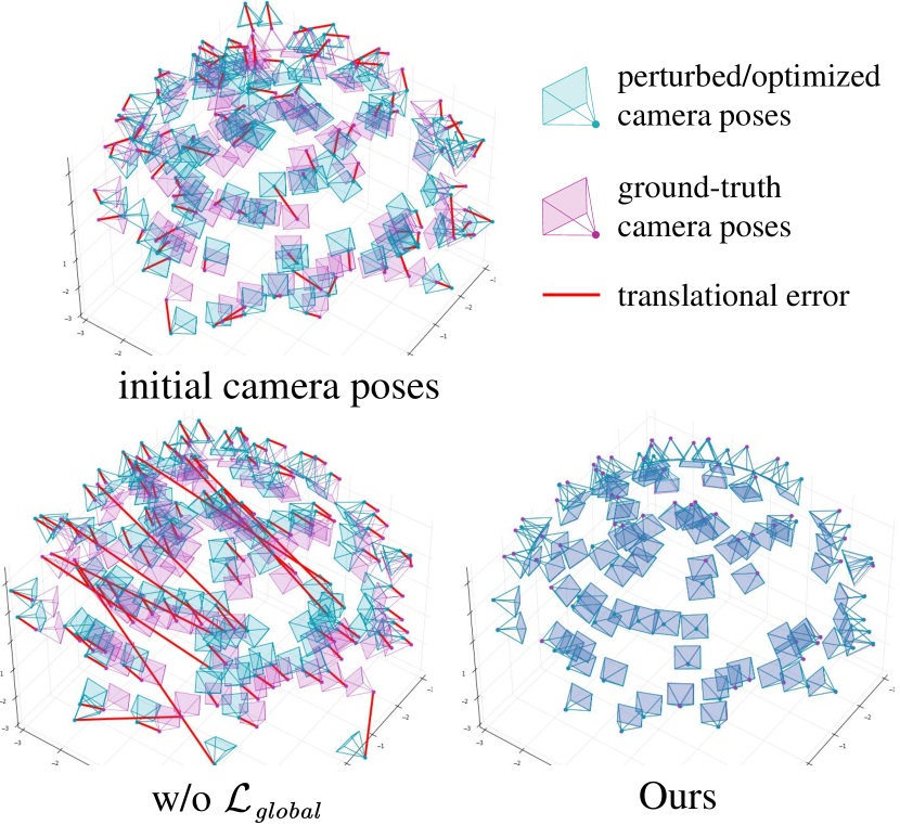
Figure 11: Visual comparison of ablation study about optimized camera poses (Procrustes aligned) for hotdog object. Full L2G-NeRF successfully aligns camera frames while w/o $\mathcal{L}_{global}$ gets stuck at suboptimal poses.

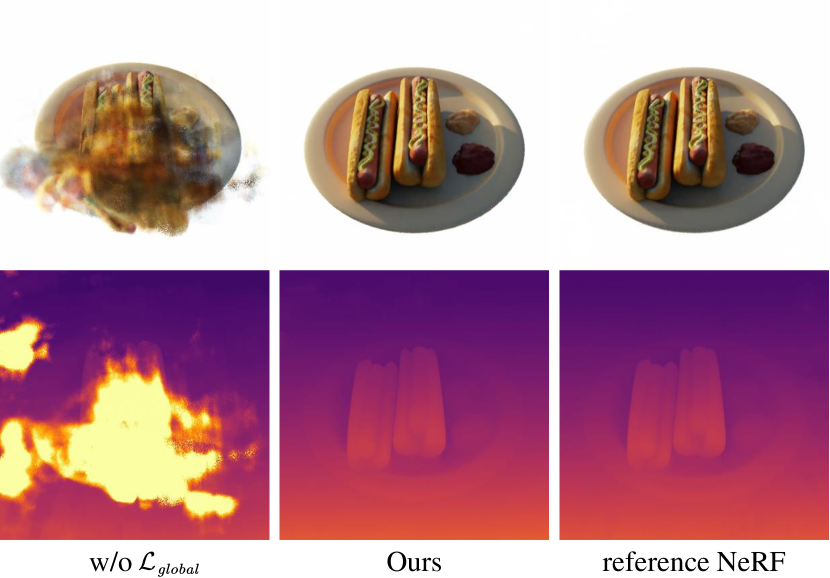
Figure 12: Ablation study of NeRF on hotdog synthetic object. The image synthesis and the expected depth are visualized with ray compositing in the top and bottom rows, respectively. Full L2G-NeRF achieves comparable rendering quality to the reference NeRF (trained using ground-truth poses), while ablation w/o $\mathcal{L}_{global}$ renders artifacts due to suboptimal registration.

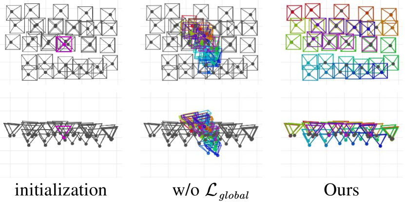
Figure 13: Visualization of ablation study about registration for room scene. Results from L2G-NeRF highly agree with SfM [37] (colored in black), whereas w/o $\mathcal{L}_{global}$ results in suboptimal alignment.

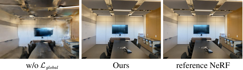
Figure 14: Ablation study of NeRF on room real-world scenes from unknown camera poses. While L2G-NeRF can jointly optimize poses and scenes, L2G-NeRF produces high fidelity results, which is competitive to reference NeRF trained using SfM poses. Ablation w/o $\mathcal{L}_{global}$ diverges to wrong poses and hence produces ghosting artifacts.

Scene	Camera pose registration						View synthesis quality
	Rotation ($\degree$) $\downarrow$			Translation $\downarrow$			PSNR $\uparrow$				SSIM $\uparrow$				LPIPS $\downarrow$
	Global	Local	L2G	Global	Local	L2G	Global	Local	L2G	ref.	Global	Local	L2G	ref.	Global	Local	L2G	ref.
	BARF	w/o $\mathcal{L}_{g}$	Ours	BARF	w/o $\mathcal{L}_{g}$	Ours	BARF	w/o $\mathcal{L}_{g}$	Ours	NeRF	BARF	w/o $\mathcal{L}_{g}$	Ours	NeRF	BARF	w/o $\mathcal{L}_{g}$	Ours	NeRF
Synthetic objects	7.02	3.63	0.15	29.84	14.34	0.61	20.51	22.70	28.62	29.42	0.82	0.85	0.93	0.94	0.22	0.14	0.07	0.06
Real-World scenes	0.55	23.82	0.46	0.33	10.66	0.32	24.23	20.71	24.54	22.44	0.73	0.64	0.75	0.65	0.23	0.33	0.20	0.29

Table 8: Quantitative results of ablation study about bundle-adjusting neural radiance fields. L2G-NeRF outperforms the local registration method (ablation w/o $\mathcal{L}_{global}$) and global registration method (BARF) on the average evaluation criteria of both synthetic objects and real-world scenes, which reveals the advantage of our local-to-global registration process. Translation errors are scaled by $100$.

A.3 Convergence

We analyze the convergence of joint optimization on the Ship scene. We first set the base rotation noise multiplier $n_{r}$ as $0.01$ and the base translation noise multiplier $n_{t}$ as $0.1$, then linearly increased them by a common factor of $\{n_{c}\}_{n_{c}=2}^{9}$. As shown in Fig. 10, BARF fails to converge with $n_{c}$=$4$ ($n_{r}$=$0.04$,$n_{t}$=$0.4$) while L2G-NeRF fails to converge with $n_{c}$=$8$ ($n_{r}$=$0.08$,$n_{t}$=$0.8$). Moreover, we also analyze the influence of individual noise. Let $n_{r}$=$0$, BARF and L2G-NeRF can handle the largest $n_{t}$ of $0.6$ and $1.1$, respectively. Let $n_{t}$=$0$, BARF and L2G-NeRF can handle the largest $n_{r}$ of $0.16$ and $0.25$, respectively. In more noisy cases (such as random init), all methods cannot converge.

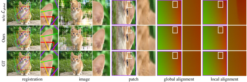
Figure 15: Ablation study of the neural image alignment experiment. Given color-coded image patches, we aim to recover the alignment and the neural field of the entire image. L2G-NeRF is able to find proper alignment and reconstruct high-fidelity neural image, while w/o $\mathcal{L}_{global}$ falls into false local alignments that do not obey the geometric constraint (global alignments), which results in ambiguous registration and distorted reconstruction (cat ears).

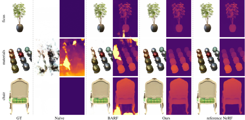
Figure 16: Additional qualitative results of bundle-adjusting neural radiance fields on synthetic scenes. The image synthesis and the expected depth are visualized with ray compositing in the left and right columns. While baselines render artifacts due to suboptimal solutions, L2G-NeRF achieves qualified visual quality, which is comparable to the reference NeRF trained using ground-truth poses.

A.4 Tuning Parameters

We set the multiplier $\lambda$ of the global alignment objective to $1\times 10^{2}$ for both the neural image alignment experiment and learning NeRF from imperfect camera poses with synthetic object-centric scenes. To further solve the challenging problem of learning NeRF in forward-facing LLFF scenes from unknown poses, we float the multiplier $\lambda$ between $1\times 10^{2}$ and $1\times 10^{5}$ (summarized in Table 6) to achieve preferable results for specific scenes. As shown in Table 7, a larger $\lambda$ encourages the model to emphasize geometric constraints more, achieving better accuracy but worse robustness (fails to converge on the Flower scene).

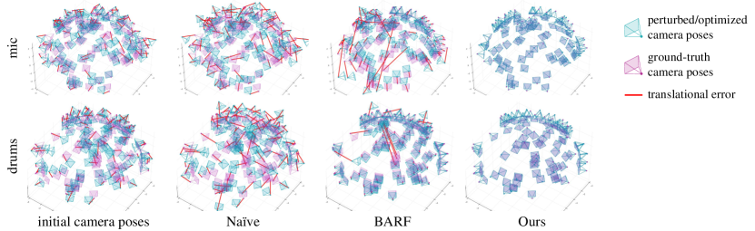
Figure 17: Additional visual comparison of the optimized camera poses (Procrustes aligned) for the mic and drums objects. L2G-NeRF successfully aligns all the camera frames while baselines get stuck at suboptimal solutions.

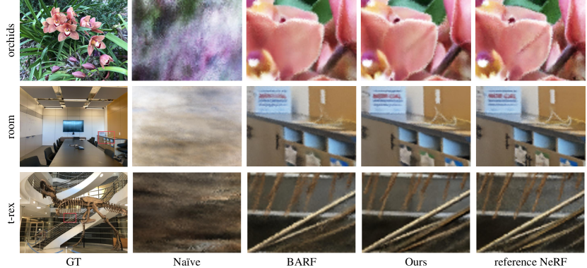
Figure 18: Additional novel view synthesis results of NeRF on real-world scenes (LLFF dataset) from unknown camera poses. L2G-NeRF can optimize for neural fields of higher quality than baselines, while achieving the comparable quality of the reference NeRF model that is trained under the camera poses provided by SfM [37].

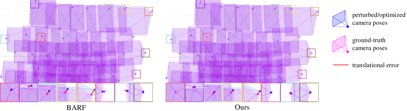
Figure 19: Visual comparison of the optimized camera poses (Procrustes aligned) for the t-rex real-world scene. L2G-NeRF successfully recovers the camera poses from identity transformation, which achieves fewer errors than BARF.

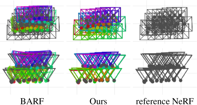
Figure 20: Visual comparison of optimized camera poses (Procrustes aligned) for the challenging toys scene captured under large displacements (hierarchical camera poses). L2G-NeRF successfully aligns all camera frames, which highly agrees with SfM [37] camera poses (colored in black), while BARF gets stuck at suboptimal solutions.

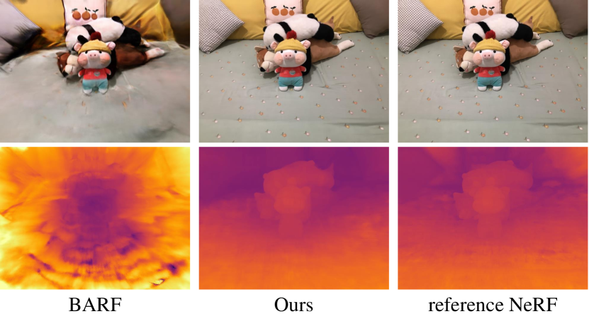
Figure 21: Results of NeRF on toys scene. L2G-NeRF achieves comparable synthesis quality to the reference NeRF (trained under SfM camera poses). But BARF fails to recover the proper geometry, which results in artifacts.

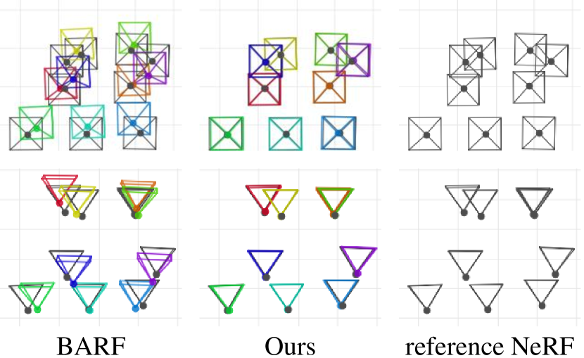
Figure 22: Visual comparison of optimized camera poses for the challenging foods scene captured under sparse views. Results from L2G-NeRF highly agree with SfM, whereas BARF results in suboptimal alignment.

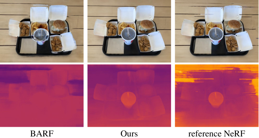
Figure 23: Results of NeRF on foods scene. L2G-NeRF outperforms BARF and even achieves better performance than reference NeRF in the scene where SfM [37] struggles with finding accurate registration from sparse views.

Scene	Camera pose registration						View synthesis quality
	Rotation ($\degree$) $\downarrow$			Translation $\downarrow$			PSNR $\uparrow$				SSIM $\uparrow$				LPIPS $\downarrow$
	Naïve	BARF	Ours	Naïve	BARF	Ours	Naïve	BARF	Ours	ref.	Naïve	BARF	Ours	ref.	Naïve	BARF	Ours	ref.
										NeRF				NeRF				NeRF
Toys	14.22	179.73	0.42	6.14	24.84	0.33	15.55	11.29	29.58	32.90	0.57	0.49	0.94	0.96	0.50	0.77	0.06	0.04
Foods	5.30	10.99	0.31	7.76	10.15	0.62	19.11	18.02	31.83	24.58	0.71	0.68	0.95	0.89	0.23	0.26	0.05	0.13

Table 9: Quantitative results of bundle-adjusting neural radiance fields on real-world scenes captured using an iPhone under large displacements (toys) or sparse views (foods). L2G-NeRF outperforms baselines and even achieves better performance than reference NeRF that trained under SfM poses in the Foods scene, which is hard for SfM to find accurate camera poses. Translation errors are scaled by $100$.

B Ablation Studies

We propose a local-to-global registration method that combines the benefits of parametric and non-parametric methods. The key idea is to apply a pixel-wise alignment that optimizes photometric reconstruction errors $\sum_{i=1}^{M}\sum^{N}_{j=1}\big{\|}\mathcal{R}(\mathbf{T}^{j}_{i}\mathbf{x}^{j};\boldsymbol{\Theta})-\mathcal{I}_{i}(\mathbf{x}^{j})\big{\|}_{2}^{2}$, followed by a frame-wise alignment $\sum_{i=1}^{M}\sum^{N}_{j=1}\lambda\big{\|}\mathbf{T}^{j}_{i}\mathbf{x}^{j}-\mathbf{T}^{\ast}_{i}\mathbf{x}^{j}\big{\|}_{2}^{2}$ to globally constrain the geometric transformations. We evaluate our proposed L2G-NeRF against an ablation (w/o $\mathcal{L}_{global}$), which builds upon our full model by eliminating the global alignment objective, i.e., $\lambda=0$. The ablation is equivalent to a local registration method, while BARF is the chosen representative global registration method.

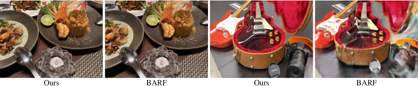
Figure 24: Results of NeRF on reflective scenes.(Shiny dataset)

B.1 Ablation on NeRF (3D): Synthetic Objects

We first investigate the ablation study of learning NeRF from imperfect camera poses. We experiment with 8 synthetic object-centric scenes [28]. The results in Fig. 12 and Table 8 show that L2G-NeRF achieves better performance than the ablation w/o $\mathcal{L}_{global}$. Fig. 11 further illustrates that L2G-NeRF can achieve near-perfect registration while the ablation w/o $\mathcal{L}_{global}$ suffers from suboptimal solutions.

B.2 Ablation on NeRF (3D): Real-World Scenes

We further explore the ablation study of learning NeRF in real-world scenes with unknown camera poses. We evaluate on the standard LLFF dataset [27]. Quantitative results are summarized in Table 8. The ablation w/o $\mathcal{L}_{global}$ diverges to wrong poses (visualized in Fig. 13), producing ghosting artifacts (shown in Fig. 14). L2G-NeRF outperforms the ablation w/o $\mathcal{L}_{global}$ and achieves high-quality view synthesis that is competitive to the reference NeRF.

B.3 Ablation on Neural Image Alignment (2D)

We further concrete analysis on the homography image alignment experiment and visualize the results in Fig. 15. Alignment with w/o $\mathcal{L}_{global}$ results in distorted artifacts (cat ears) in the recovered neural image due to ambiguous registration. This is the consequence of w/o $\mathcal{L}_{global}$’s attempt to directly optimize the pixel agreement metric, which minimizes photometric errors but does not obey the geometric constraint (global alignments). As L2G-NeRF discovers precise warps, it optimizes neural image with high fidelity.

C Additional Results

C.1 NeRF (3D): Synthetic Objects

We report additional qualitative results of learning NeRF from noisy camera poses for synthetic objects in Fig. 16. The baselines still perform poorly, while L2G-NeRF can achieve near-perfect registration (reflected in Fig. 17) and render images with comparable visual quality against reference NeRF that trained under ground-truth poses.

C.2 NeRF (3D): Real-World Scenes (LLFF)

We report additional qualitative results of learning NeRF for the standard LLFF dataset in Fig. 18, where camera poses are unknown. L2G-NeRF successfully recovers the 3D scene with higher fidelity than baselines. Fig. 19 shows that the recovered camera poses from L2G-NeRF agree more with those estimated from SfM methods than BARF.

C.3 NeRF (3D): Real-World Scenes (Ours)

We take one step further to experiment with images captured using an iPhone under challenging camera pose distribution. Fig. 20 and Fig. 22 indicate the advantage of L2G-NeRF in registering images captured under large displacements and sparse views, while baselines exhibit artifacts (Fig. 21 and Fig. 23) due to unreliable registration, which is reflected in Table 9. Moreover, the difficulty of registering from sparse views prevents SfM from finding accurate poses, which results in broken stripes on the synthesis of reference NeRF trained under SfM poses in foods scene. This further demonstrates the effectiveness of removing the requirement of pre-computed SfM poses. Fig. 20 and Fig. 22 show the largest displacements (hierarchical but adjacent camera poses) and the sparsest camera setting (9 views) of L2G-NeRF to register images in these scenes successfully, than which we can not handle a more challenging camera pose distribution.

C.4 NeRF (3D): Real-World Scenes (Shiny)

To analyze the influence of reflective surfaces, We present an example in Fig. 24 that reconstructs scenes  [45] with reflections from identity pose initialization (L2G-NeRF converges, BARF fails in the guitars scene). Interestingly, the global alignment loss increases by 4 to 10 times w.r.t. other datasets. This may be caused by inaccurate local registration in specular regions, and our convergence benefits from the global registration constraint. Specific methods (e.g., Ref-NeRF [42]) could be employed to handle reflective surfaces better.

References

- [1] Yousset I Abdel-Aziz, Hauck Michael Karara, and Michael Hauck. Direct linear transformation from comparator coordinates into object space coordinates in close-range photogrammetry. Photogrammetric engineering & remote sensing, 81(2):103–107, 2015.
- [2] Sameer Agarwal, Yasutaka Furukawa, Noah Snavely, Ian Simon, Brian Curless, Steven M Seitz, and Richard Szeliski. Building rome in a day. ACM Communications, 2011.
- [3] Hatem Alismail, Brett Browning, and Simon Lucey. Photometric bundle adjustment for vision-based slam. In Asian Conference on Computer Vision, pages 324–341. Springer, 2016.
- [4] Mojtaba Bemana, Karol Myszkowski, Hans-Peter Seidel, and Tobias Ritschel. X-fields: Implicit neural view-, light-and time-image interpolation. ACM Transactions on Graphics (TOG), 39(6):1–15, 2020.
- [5] Xingyu Chen, Qi Zhang, Xiaoyu Li, Yue Chen, Ying Feng, Xuan Wang, and Jue Wang. Hallucinated neural radiance fields in the wild. In Proceedings of the IEEE/CVF Conference on Computer Vision and Pattern Recognition, pages 12943–12952, 2022.
- [6] Yinbo Chen, Sifei Liu, and Xiaolong Wang. Learning continuous image representation with local implicit image function. In Proceedings of the IEEE/CVF conference on computer vision and pattern recognition, pages 8628–8638, 2021.
- [7] Yue Chen, Xuan Wang, Qi Zhang, Xiaoyu Li, Xingyu Chen, Yu Guo, Jue Wang, and Fei Wang. UV Volumes for real-time rendering of editable free-view human performance. arXiv preprint arXiv:2203.14402, 2022.
- [8] Zhiqin Chen and Hao Zhang. Learning implicit fields for generative shape modeling. In Proceedings of the IEEE/CVF Conference on Computer Vision and Pattern Recognition, pages 5939–5948, 2019.
- [9] Shin-Fang Chng, Sameera Ramasinghe, Jamie Sherrah, and Simon Lucey. Gaussian activated neural radiance fields for high fidelity reconstruction and pose estimation. In European Conference on Computer Vision, pages 264–280. Springer, 2022.
- [10] Andrew J Davison, Ian D Reid, Nicholas D Molton, and Olivier Stasse. Monoslam: Real-time single camera slam. IEEE Transactions on Pattern Analysis and Machine Intelligence, 2007.
- [11] Amaël Delaunoy and Marc Pollefeys. Photometric bundle adjustment for dense multi-view 3d modeling. In Proceedings of the IEEE Conference on Computer Vision and Pattern Recognition, pages 1486–1493, 2014.
- [12] Jia Deng, Wei Dong, Richard Socher, Li-Jia Li, Kai Li, and Li Fei-Fei. Imagenet: A large-scale hierarchical image database. In Proceedings of the IEEE/CVF Conference on Computer Vision and Pattern Recognition, pages 248–255. Ieee, 2009.
- [13] Daniel DeTone, Tomasz Malisiewicz, and Andrew Rabinovich. Deep image homography estimation. arXiv preprint arXiv:1606.03798, 2016.
- [14] Jakob Engel, Vladlen Koltun, and Daniel Cremers. Direct sparse odometry. IEEE Transactions on Pattern Analysis and Machine Intelligence, 2017.
- [15] Jakob Engel, Thomas Schöps, and Daniel Cremers. Lsd-slam: Large-scale direct monocular slam. In European conference on computer vision, pages 834–849. Springer, 2014.
- [16] Richard Hartley and Andrew Zisserman. Multiple View Geometry in Computer Vision. Cambridge University Press, ISBN: 0521540518, second edition, 2004.
- [17] Xin Huang, Qi Zhang, Ying Feng, Hongdong Li, Xuan Wang, and Qing Wang. Hdr-nerf: High dynamic range neural radiance fields. In Proceedings of the IEEE/CVF Conference on Computer Vision and Pattern Recognition, pages 18398–18408, 2022.
- [18] John R Hurley and Raymond B Cattell. The procrustes program: Producing direct rotation to test a hypothesized factor structure. Behavioral science, 7(2):258, 1962.
- [19] Yoonwoo Jeong, Seokjun Ahn, Christopher Choy, Anima Anandkumar, Minsu Cho, and Jaesik Park. Self-calibrating neural radiance fields. In Proceedings of the IEEE/CVF International Conference on Computer Vision, pages 5846–5854, 2021.
- [20] Wolfgang Kabsch. A solution for the best rotation to relate two sets of vectors. Acta Crystallographica Section A: Crystal Physics, Diffraction, Theoretical and General Crystallography, 32(5):922–923, 1976.
- [21] Yoni Kasten, Dolev Ofri, Oliver Wang, and Tali Dekel. Layered neural atlases for consistent video editing. ACM Transactions on Graphics (TOG), 40(6):1–12, 2021.
- [22] Hoang Le, Feng Liu, Shu Zhang, and Aseem Agarwala. Deep homography estimation for dynamic scenes. In Proceedings of the IEEE/CVF Conference on Computer Vision and Pattern Recognition, pages 7652–7661, 2020.
- [23] Chen-Hsuan Lin, Wei-Chiu Ma, Antonio Torralba, and Simon Lucey. BARF: Bundle-adjusting neural radiance fields. In Proceedings of the IEEE/CVF International Conference on Computer Vision, pages 5741–5751, 2021.
- [24] Chen-Hsuan Lin, Oliver Wang, Bryan C Russell, Eli Shechtman, Vladimir G Kim, Matthew Fisher, and Simon Lucey. Photometric mesh optimization for video-aligned 3d object reconstruction. In Proceedings of the IEEE/CVF Conference on Computer Vision and Pattern Recognition, 2019.
- [25] Quan Meng, Anpei Chen, Haimin Luo, Minye Wu, Hao Su, Lan Xu, Xuming He, and Jingyi Yu. Gnerf: Gan-based neural radiance field without posed camera. In Proceedings of the IEEE/CVF International Conference on Computer Vision, pages 6351–6361, 2021.
- [26] Lars Mescheder, Michael Oechsle, Michael Niemeyer, Sebastian Nowozin, and Andreas Geiger. Occupancy networks: Learning 3d reconstruction in function space. In Proceedings of the IEEE/CVF conference on computer vision and pattern recognition, pages 4460–4470, 2019.
- [27] Ben Mildenhall, Pratul P Srinivasan, Rodrigo Ortiz-Cayon, Nima Khademi Kalantari, Ravi Ramamoorthi, Ren Ng, and Abhishek Kar. Local light field fusion: Practical view synthesis with prescriptive sampling guidelines. ACM Transactions on Graphics (TOG), 38(4):1–14, 2019.
- [28] Ben Mildenhall, Pratul P Srinivasan, Matthew Tancik, Jonathan T Barron, Ravi Ramamoorthi, and Ren Ng. Nerf: Representing scenes as neural radiance fields for view synthesis. In European conference on computer vision, 2020.
- [29] Raul Mur-Artal, Jose Maria Martinez Montiel, and Juan D Tardos. Orb-slam: a versatile and accurate monocular slam system. IEEE transactions on robotics, 31(5):1147–1163, 2015.
- [30] Seonghyeon Nam, Marcus A Brubaker, and Michael S Brown. Neural image representations for multi-image fusion and layer separation. In European conference on computer vision, 2022.
- [31] Richard A Newcombe, Steven J Lovegrove, and Andrew J Davison. Dtam: Dense tracking and mapping in real-time. In Proceedings of the IEEE International Conference on Computer Vision, 2011.
- [32] Michael Niemeyer and Andreas Geiger. Giraffe: Representing scenes as compositional generative neural feature fields. In Proceedings of the IEEE/CVF Conference on Computer Vision and Pattern Recognition, pages 11453–11464, 2021.
- [33] Jeong Joon Park, Peter Florence, Julian Straub, Richard Newcombe, and Steven Lovegrove. Deepsdf: Learning continuous signed distance functions for shape representation. In Proceedings of the IEEE/CVF conference on computer vision and pattern recognition, pages 165–174, 2019.
- [34] Sida Peng, Yuanqing Zhang, Yinghao Xu, Qianqian Wang, Qing Shuai, Hujun Bao, and Xiaowei Zhou. Neural body: Implicit neural representations with structured latent codes for novel view synthesis of dynamic humans. In Proceedings of the IEEE/CVF Conference on Computer Vision and Pattern Recognition, pages 9054–9063, 2021.
- [35] Marc Pollefeys, Reinhard Koch, and Luc Van Gool. Self-calibration and metric reconstruction inspite of varying and unknown intrinsic camera parameters. International Journal of Computer Vision, 32(1):7–25, 1999.
- [36] Marc Pollefeys, Luc Van Gool, Maarten Vergauwen, Frank Verbiest, Kurt Cornelis, Jan Tops, and Reinhard Koch. Visual modeling with a hand-held camera. International Journal of Computer Vision, 59(3):207–232, 2004.
- [37] Johannes L Schonberger and Jan-Michael Frahm. Structure-from-motion revisited. In Proceedings of the IEEE conference on computer vision and pattern recognition, pages 4104–4113, 2016.
- [38] Vincent Sitzmann, Julien Martel, Alexander Bergman, David Lindell, and Gordon Wetzstein. Implicit neural representations with periodic activation functions. Advances in Neural Information Processing Systems, 33:7462–7473, 2020.
- [39] Noah Snavely, Steven M Seitz, and Richard Szeliski. Photo tourism: exploring photo collections in 3d. In SIGGRAPH Conference Proceedings. 2006.
- [40] Noah Snavely, Steven M Seitz, and Richard Szeliski. Modeling the world from internet photo collections. International journal of computer vision, 2008.
- [41] Shinji Umeyama. Least-squares estimation of transformation parameters between two point patterns. IEEE Transactions on Pattern Analysis & Machine Intelligence, 13(04):376–380, 1991.
- [42] Dor Verbin, Peter Hedman, Ben Mildenhall, Todd Zickler, Jonathan T Barron, and Pratul P Srinivasan. Ref-nerf: Structured view-dependent appearance for neural radiance fields. In Proceedings of the IEEE conference on computer vision and pattern recognition, pages 5481–5490. IEEE, 2022.
- [43] Zirui Wang, Shangzhe Wu, Weidi Xie, Min Chen, and Victor Adrian Prisacariu. NeRF: Neural radiance fields without known camera parameters. arXiv preprint arXiv:2102.07064, 2021.
- [44] Chung-Yi Weng, Brian Curless, Pratul P Srinivasan, Jonathan T Barron, and Ira Kemelmacher-Shlizerman. Humannerf: Free-viewpoint rendering of moving people from monocular video. In Proceedings of the IEEE/CVF Conference on Computer Vision and Pattern Recognition, pages 16210–16220, 2022.
- [45] Suttisak Wizadwongsa, Pakkapon Phongthawee, Jiraphon Yenphraphai, and Supasorn Suwajanakorn. Nex: Real-time view synthesis with neural basis expansion. In Proceedings of the IEEE conference on computer vision and pattern recognition, 2021.
- [46] Yitong Xia, Hao Tang, Radu Timofte, and Luc Van Gool. Sinerf: Sinusoidal neural radiance fields for joint pose estimation and scene reconstruction. British Machine Vision Conference, 2022.
- [47] Yiheng Xie, Towaki Takikawa, Shunsuke Saito, Or Litany, Shiqin Yan, Numair Khan, Federico Tombari, James Tompkin, Vincent Sitzmann, and Srinath Sridhar. Neural fields in visual computing and beyond. In Computer Graphics Forum, volume 41, pages 641–676, 2022.
- [48] Anqi Joyce Yang, Can Cui, Ioan Andrei Bârsan, Raquel Urtasun, and Shenlong Wang. Asynchronous multi-view SLAM. In IEEE International Conference on Robotics and Automation (ICRA), 2021.
- [49] Lin Yen-Chen, Pete Florence, Jonathan T Barron, Alberto Rodriguez, Phillip Isola, and Tsung-Yi Lin. inerf: Inverting neural radiance fields for pose estimation. In 2021 IEEE/RSJ International Conference on Intelligent Robots and Systems (IROS), pages 1323–1330. IEEE, 2021.
- [50] Richard Zhang, Phillip Isola, Alexei A Efros, Eli Shechtman, and Oliver Wang. The unreasonable effectiveness of deep features as a perceptual metric. In Proceedings of the IEEE conference on computer vision and pattern recognition, pages 586–595, 2018.