secReference
Robust and Efficient Network Reconstruction in Complex System
via Adaptive Signal Lasso
Abstract
Network reconstruction is important to the understanding and control of collective dynamics in complex systems. Most real networks exhibit sparsely connected properties, and the connection parameter is a signal (0 or 1). Well-known shrinkage methods such as lasso or compressed sensing (CS) to recover structures of complex networks cannot suitably reveal such a property; therefore, the signal lasso method was proposed recently to solve the network reconstruction problem and was found to outperform lasso and CS methods. However, signal lasso suffers the problem that the estimated coefficients that fall between 0 and 1 cannot be successfully selected to the correct class. We propose a new method, adaptive signal lasso, to estimate the signal parameter and uncover the topology of complex networks with a small number of observations. The proposed method has three advantages: (1) It can effectively uncover the network topology with high accuracy and is capable of completely shrinking the signal parameter to either 0 or 1, which eliminates the unclassified portion in network reconstruction; (2) The method performs well in scenarios of both sparse and dense signals and is robust to noise contamination; (3) The method only needs to select one tuning parameter versus two in signal lasso, which greatly reduces the computational cost and is easy to apply. The theoretical properties of this method are studied, and numerical simulations from linear regression, evolutionary games, and Kuramoto models are explored. The method is illustrated with real-world examples from a human behavioral experiment and a world trade web.
Keywords: network reconstruction, sparsity, signal lasso, adaptive signal lasso, evolutionary game, synchronization model
I Introduction
Complex networks have wide applications and seen much progress Strogatz (2001); Barabási (2012); Albert and Barabási (2002); Boccaletti et al. (2006). In a complex network, the pattern of node-to-node interaction or network topology is unknown. To uncover the network topology based on a series of observable quantities obtained from experiments or observations is important and may play a role in the understanding and controlling of collective dynamics of complex systems Han et al. (2015); Wang et al. (2011); Peixoto (2018). Network reconstruction as an inverse problem in network science has been paid much attention recently, such as in the reconstruction of gene networks using expression data Gardner et al. (2003); Geier et al. (2007), extraction of various functional networks in the human brain from activation data Grün et al. (2002); Supekar et al. (2008), and detection of organizational networks in social science and trade networks in economics Squartini et al. (2018). Evolutionary game-based dynamics have been used to study network reconstruction, where it is possible to observe a series of a small number of discrete quantities Wang et al. (2011); Han et al. (2015); Shi et al. (2020a, 2021), in which case the problem can be transformed to a statistical linear model with sparse and high-dimensional properties.
We use two typical examples to illustrate how such signal parameters appear in practice. The first example is a dynamic equation governing the evolution state in a general complex system, which can be written as differential equations Wang et al. (2016); Raimondo and Domenico (2021)
| (1) |
where denotes an -dimensional internal state variable of a system consisting of dynamic units at time , where and , respectively, define the intrinsic and interaction dynamics of the units; is a dynamic noise term; is a set of dynamic parameters; and defines the interaction topology and is called by an adjacency matrix such that = 1 if there is a direct physical interaction from unit to , and = 0 otherwise. The matrix completely defines a network with size , i.e., an abstraction used to model a system that contains discrete interconnected elements. The elements are represented by nodes (also called vertices), and connections by edges. In general, can be observed as time-series data, but for are unknown and must be estimated. It is clear that Eq. (1) can be rewritten as a linear regression model if the functional forms of and are known. This model includes synchronization models, oscillator networks, and spreading networks Wang et al. (2016).
The second example comes from the evolutionary game on structured populations, where a node represents a player, and a link indicates that two players have a game relationship. The prisoner’s dilemma game (PDG), snowdrift game (SDG), or spatial ultimatum game (SUG) can be used for network reconstruction Wang et al. (2011); Han et al. (2015); Peixoto (2018); Shi et al. (2021). We use the PDG, with temptation to defect , reward for mutual cooperation , punishment for mutual defection , and sucker’s payoff . Thus, the payoff matrices can be defined as
| (2) |
and , where mutual defections are the equilibrium solutions Santos and Pacheco (2005); Nowak and May (1992); Hauert and Doebeli (2004); Szabó and Fath (2007). For simplicity, these parameters are re-scaled as , , and , where ensures a proper payoff ranking () and captures the essential social dilemma Nowak and May (1992); Perc et al. (2017). In some experimental driving studies, each player can interact with other players by choosing either a cooperator (C) or defector (D) to obtain their payoff and the procedure is continued for a predetermined number of roundsLi et al. (2018); Wang et al. (2017, 2018); Shi et al. (2020b). In a theoretical study, some updating mechanism can be used to generate theoretical data on three types of topologies Szabó et al. (2005). Suppose that each player is either a cooperator (C) or defector (D) with equal probability, which can be written as or . In a spatial PDG game, player , say the focal player, acquires its fitness (total payoff) by playing the game with all its connected neighbors,
| (3) |
where is the set of all connected neighbors of player , . Eq. (3) can be converted to a linear model, with elements of the adjacency matrix for a network. If , then players and are connected, and if , then they are not. The process can produce time-series data. In each step, players can update their strategies using a rule, or determine them themselves. Suppose accessible time is available. Then, the model containing the time-series data can be rewritten as
| (4) |
where , , and , in which the th connection with itself is removed. The introduction of is due to noises or missing nodes in real applications. Therefore the aim of Eq. (4) is to estimate the elements of the connectivity matrix, which is important for uncovering network structures, such as possible social network in the social science or an intrinsic scientific relationship in gene-regulatory network reconstruction from the expression data in systems biology.
In the areas of complex systems and applied physics, the compressed sensing (CS) or lasso methods are techniques to estimate and achieve the purpose of network reconstruction Wang et al. (2011); Han et al. (2015); Shi et al. (2020a), and lasso has been found to be robust against noises in the reconstruction of sparse signals. Player and player are predicted to have a game relationship (connection) if , and no relationship if , where is an estimator of . Otherwise, the relationship is not identifiable. Although the CS or lasso method can shrink parameter estimates toward zero under natural sparsity in complex networks, links between nodes cannot be shrunk to a true value of 1, which will decrease estimation accuracy in most cases. For this reason, Shi et al. (2021) Shi et al. (2021) proposed the signal lasso method to solve the network reconstruction problem and found that it performed better than the lasso and CS methods. However values of that fall in the interval (0.1,0.9) cannot be placed in the correct class and leave an unclassified portion in network reconstruction.
We propose a method called adaptive signal lasso to estimate the signal parameter and uncover the topology in complex networks with a small number of observations. The idea is to add weights to the penalty terms of signal lasso. We show that our method can shrink the parameter to either 0 or 1 completely and greatly improve estimation accuracy. Furthermore, this method only tunes one parameter in a very small range, which saves computation time. The method is robust against noise and missing nodes, since a least square error control term is included. We conduct simulations and comparison studies through a linear regression model with signal parameters using six current shrinkage methods and our proposed method. We validate our reconstruction framework through an evolutionary game and synchronization model by considering three topological structures: random (ER), small word, and scale-free. The results show that our method can achieve high prediction accuracy compared with the other methods, remove the unclassified portion of subjects, and decrease the computational cost. We use two real examples for illustration and find that our method performs surprisingly well at detecting signals in all cases (including case of dense networks). Our method has potential applications in fields such as social, economic, physical, and biological systems, and the recovery of hidden networks.
II Motivation
Consider the general linear regression model
| (5) |
where is a noise or random error with mean zero and finite variance, is an matrix, is an vector, and is a unknown vector. To eliminate the intercept from (5), throughout this paper, we center the response and predictor variables so that the mean of the response is zero. We assume the parameter has a signal property, e.g., the true values of , , are either 0 or 1. This kind of problem is common in the reconstruction of complex networks to identify a signal as either connected or not Han et al. (2015); Wang et al. (2011).
The signal lasso method minimizes Shi et al. (2021)
| (6) |
where are two tuning parameters. The term is added in the penalty term because some elements of should be 1. When , it reduces to the lasso method Tibshirani (1996). The tuning parameters and must be determined by the dataset through cross-validation. This is a compromise between shrinking terms to 0 and 1, and we expect some elements of will be close to 0, and others to 1.
If the columns of are orthogonal to each other and , denoting the ordinary least squares estimate by , the estimator of in signal lasso is
| (7) |
for , where and , and and are the th element of and , respectively; denote the positive part of , it means that if and 0 otherwise. is similarly defined as the negative part of .
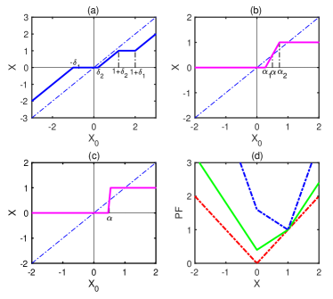
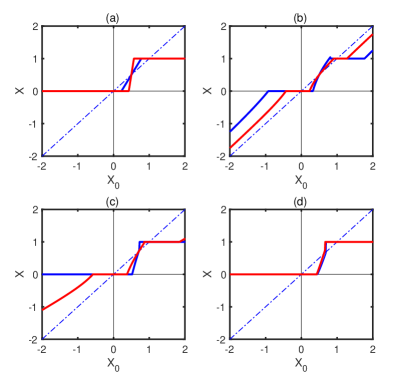
Fig. 1 (a) shows the solutions of as a function of under an orthogonal design matrix for the signal lasso method, where and , and the line of is for reference. The signal lasso method not only shrinks the small values of the parameter to zero but also shrinks large values to 1, and therefore outperforms the lasso and CS methods in network reconstruction for signal parameters Shi et al. (2021). However, this method still has some unsatisfactory aspects in shrinking signal parameters. First, although larger values such that can be shrunk to 1, and values in the interval to 0, values in the interval only shift by a constant , making some parameters unidentifiable.
Compared to the pattern shown in Fig. 1a, the pattern shown in Fig. 1(b) and (c), obtained from our new method, is more favorable, as the middle part between 0 and 1 can be shrunk toward to two directions. Second, signal lasso involves two tuning parameters, making the computation costly even if cross-validation is available. To overcome these weaknesses, we propose an efficient modification by given a weight in penalized terms of signal lasso. We find that the estimation of parameters in model in (5) can be completely shrunk to 0 or 1, and we only need to select one tuning parameter, which makes the computation fast and greatly improves its accuracy.
III Adaptive signal lasso
III.1 Method
To deal with the abovementioned problems, we propose following penalized least square function
| (8) |
with the penalty function given by
where weight coefficients and are functions of , an initial estimator of , which can be an ordinary least square estimator for , or a ridge estimator for . A new estimator of defined by
| (9) |
is called adaptive signal lasso. For the choice of weights, we expect that the first term of the penalty will have a lower weight, and the second term will have a large weight when is close to (similar to when is close to ). Motivated by adaptive lasso, we can choose that
with for . After comparison and analysis, we find the best candidates for the weights are and . This is effective in the analysis and will be used throughout this paper if not specified otherwise (see Appendix 1 for discussions).
Now, we give the geometry of adaptive signal lasso in the case of an orthogonal design matrix with . After some calculations (see Appendix 2), the solution is given by
| (10) |
where . In this case, adaptive signal lasso with will enjoy satisfactory technical properties. Fig. 1(b) shows the solutions of as a function of for adaptive signal lasso in the special case of (10), where the main difference from signal lasso occurs in the interval (0,1). It is of interest to see that the values of in will be shrunk toward 0, while the values of will be shrunk toward 1, where and . The line has a slope of , which indicates a kind of shrinkage strength. When increases to 12 and we keep (which means ), the pattern given in Fig. 1(c) shows that almost all parameter estimation in the middle part can be shrunk almost to 0 or 1.
Thus we re-parameterize and by and and rewrite the the penalty function by
| (11) |
It can be easily proved from Eq (10) that when is fixed and let , then we have
| (12) |
since and in these scenarios. The parameter can be assigned randomly as 0 or 1 if . This result indicates that if we set large enough, the estimators from adaptive signal lasso can be completely shrunk to either 0 or 1, thus removing the unidentified set that will be presented in the signal lasso method. Another advantage is that we only need to select tuning parameter , which dramatically reduces the computation time comparing with signal lasso. In addition, the range for selecting can be set in a small interval such as , since a smaller or larger is inappropriate in practice. If we do not like tuning the parameter, a rough value of is preferable in most cases in adaptive signal lasso. Fig. 1 (d) shows the functional form of the penalty to show how the penalties behave for different values of . For example, when , the adaptive penalty function tends to shrink toward (0,1), while it shrinks toward (1,0) when .
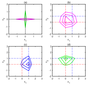
Fig. 2 shows constraint regions for different shrink estimation methods. Fig. 2 (a) shows the graphs for adaptive lasso methods. Fig. 2 (b) shows signal lasso and Fig. 1 (c)–(d) show adaptive signal lasso with different values of . For example, for , the contours for adaptive signal lasso will be centered at , gradually converging to it when becomes small. It is of interest to see that the shape of constraint regions in adaptive signal lasso varies by target point.
III.2 Algorithm and computation
It is noted that the penalty function in Eq (8) is convex. Hence, the optimization problem in (9) does not suffer from multiple local minima, and its global minimizer can be efficiently solved. We provide an algorithm using the coordinate descent method Hastie et al. (2015), an iterative algorithm that updates the estimator by choosing a single coordinate to update, and then performing a univariate minimization over it. Since and are known, we denote , . Define a threshold function by
| (13) |
Then, the update can proceed as
| (14) |
where , , denotes the inner product of vectors and , is the th column of , is the estimator of in the th step, and . The algorithm applies this update repeatedly in a cyclical manner, updating the coordinates of along the way. Once an initial estimator of is given, for example by lasso or ridge estimation, updating can continue until convergence. These results are proved in Appendix 2.
If Eq. (9) is formulated by parameters and and , , then
Let . It is clear that Eq. (14) will shrink the negative solution to 0 ,and a solution larger than 1 to 1, because . For , when and , then and only the last condition in Eq. (13) holds. Therefore, the solution gives a result of 1, since in this case. When and , then , and only the first two conditions in Eq.(13) are possible. However, they both equal 0 since . This indicates that the conclusion given in Eq. (10) still holds in the general case, which will be helpful for selecting the tuning parameters in adaptive signal lasso.
III.3 Tuning the parameter
From the previously mentioned properties based on and in Eq.(11), we can specify a large value for and only tune using cross-validation (CV), which only involves one parameter and will greatly reduce computation. Furthermore, since represents the proportion of data compressed to 0 in the interval (0, 1), it should be less than 1 and greater than 0. In practical situations, too small or large an is not preferable; hence an empirical treatment is to select in a small interval such as (0.2,0.8). Our simulation confirms this is enough to conduct cross-validation. In addition, if one does not like to tune the parameter in adaptive signal lasso, an approximate value of can be used. We use as a large value, and find it is good enough in our calculations, and remove the unclassified portion in network reconstruction.
| Actual class | Predicted class | |||
|---|---|---|---|---|
| Signal | Non signal | Unclassified | ||
| Signal class | True positive (TP) | False negative (FN) | Unclassified positive (UCP) | |
| Non signal class | False positive (FP) | True negative (TN) | Unclassified negative (UCN) | |
III.4 The metrics of reconstruction accuracy
To measure the accuracy of the estimation method, we have to define some metrics in the signal identification problem. As shown in Table 1, we adopt common notation as in binary classification, where true positive (TP) is the number of correctly identified true signals, true negative (TN) is the number of correctly identified non-signals, false positive (FP) is the number of non-signals incorrectly identified as signals, and false negative (FN) is the number of signals incorrectly identified as non-signals. However, in our analysis, some lasso-type methods have points that cannot be classified (e.g., the parameter is classified as signal if , and non-signal if , and the remainder are unclassified Wang et al. (2011); Han et al. (2015); Shi et al. (2021)); hence, we have the additional classes of unclassified positive (UCP) and unclassified negative (UCN), as shown in Table 1. In traditional classification problems, the predicted class are completely classified to two classes, therefore most common indexes for measuring accuracies are the true positive rate (TPR, sensitivity or recall), true negative rate (TNR, or specificity) and precision (Positive prediction value, PPV ), as well as the area under the receiver operating characteristic curve (AUROC) and the area under the precision recall curve (AUPR)Marbach et al. (2012); Han et al. (2015); Squartini et al. (2018), where TPR and TNR are defined by
| (15) |
However, these measures have a problem when size of signals and non-signals are unbalanced Chicco (2017). An alternative solution employs the Matthews correlation coefficient,
| (16) |
which correctly takes into account the size of the confusion matrix elements Chicco (2017); Chicco and Jurman (2020). MCC is widely used in machine learning to measure the quality of binary classifiers and is an overall measure of accuracy at the detection of signal and non-signal classes. It is generally regarded as a balanced measure, which can be used even if classes have very different sizes Chicco and Jurman (2020); Fan et al. (2009). Its values range from -1 to 1, and a large value indicates good performance.
In most cases of network construction, some links are unclassified; hence, the success rates for the detection of existing links (SREL) and non-existing links (SRNL) are defined to study the performance of network reconstruction Wang et al. (2011); Han et al. (2015); Shi et al. (2021), where
| (17) |
which considers the effects of non-classifiability in Table 1 and is more reasonable for measuring the reconstruction accuracy of a network structure.
To address the effect of non-classifiability on accuracy measures of reconstruction, we define an adjusted MCC, MCCa, by replacing FN with FN+UCP (i.e., the number of signals that are not correctly predicted) and FP with FP+UCN (the number of incorrectly predicted non-signals) in MCC. It is clear when an unclassified set disappears, MCCa reduces to MCC. It is easy to see that MCCa plays a similar role to MCC when non-classifiability occurs. We find that MCCa performs well in network reconstruction to measure the accuracy of the method from either simulations or real examples.
IV Numerical Studies
We conduct simulation studies using three kinds of model: (1) standard linear regression model with different assumptions; (2) dynamics model of an evolutionary game Shi et al. (2021), but with the PDG game; and (3) the Kuromato model in synchronization dynamic, which is a special case of Eq. (2). Models (2) and (3) use three network topology structures: Erdös-Rényi (ER) random networks, Barabási-Albert (BA) scale-free networks, and small-world Watts-Strogatz (WS) networks. In each case, we evaluate performance under situations of sparse and dense signals.
IV.1 Linear regression models
The generation model is given by
| (18) |
where is the intercept, is an vector with all elements equal to 1, denotes the signal parameter with elements of 1, denotes the non-signal parameter with elements of 0, and is the error term. A smaller is called a sparse signal, and a larger (comparing with n and ) is called a dense signal. Each design matrix comes from a standard normal score with mean 0 and variance 1, but the columns in are correlated in such a way that the correlation coefficient between and is given by with Tibshirani (1996); Fan and Li (2001). The error variable is generated from a Gaussian distribution with mean zero and variance . We also calculate the results from several well-known shrinkage estimates, including lasso, adaptive lasso, elastic net, SCAD, MCP, and signal lasso Hastie et al. (2015); Fan and Li (2001); Shi et al. (2021). The abovementioned first five methods do not shrink the parameter in the model to 1, as they were designed to shrink irrelevant variables to zero, using different penalty functions. Hence, we call these by lasso-type methods, while signal lasso and adaptive signal lasso are called by signal-lasso-type method in this paper.
| Method | MSE/SREL/SRNL/TPR/TNR/UCR/MCC/MCCa | |
| lasso | 0.0014/0.920/0.987/0.999/1.000/0.027/1.000/0.919 | 0.0083/0.492/0.850/0.979/0.999/0.221/0.980/0.347 |
| A-lasso | 0.0015/0.925/0.976/0.999/1.000/0.343/1.000/0.900 | 0.0095/0.465/0.843/0.980/1.000/0.232/0.985/0.316 |
| SCAD | 0.0008/0.937/0.987/0.999/1.000/0.023/1.000/0.937 | 0.0043/0.522/0.985/0.999/1.000/0.108/1.000/0.632 |
| MCP | 0.0008/0.935/0.992/1.000/1.000/0.019/1.000/0.943 | 0.0046/0.525/0.980/1.000/1.000/0.111/1.000/0.633 |
| ElasticNet | 0.0012/0.835/0.999/1.000/1.000/0.333/1.000/0.892 | 0.0066/0.385/0.979/0.970/1.000/0.139/0.970/0.503 |
| S-lasso | 0.0007/0.972/0.992/0.999/1.000/0.012/1.000/0.966 | 0.0046/0.671/0.916/0.999/1.000/0.133/1.000/0.609 |
| AS-lasso | 0.0001/1.000/0.997/0.999/1.000/0.002/1.000/0.993 | 0.0006/0.980/0.990/0.999/1.000/0.012/1.000/0.965 |
| lasso | 0.0016/0.640/0.969/0.989/1.000/0.043/0.990/0.529 | 0.0085/0.333/0.859/0.969/1.000/0.162/0.970/0.107 |
| A-lasso | 0.0026/0.585/0.937/0.979/1.000/0.076/0.980/0.375 | 0.0130/0.288/0.830/0.859/1.000/0.191/0.860/0.061 |
| SCAD | 0.0002/0.822/1.000/0.999/1.000/0.007/1.000/0.896 | 0.0111/0.271/0.987/0.567/1.000/0.037/0.609/0.305 |
| MCP | 0.0002/0.820/0.999/1.000/1.000/0.007/1.000/0.892 | 0.0130/0.246/0.991/0.541/1.000/0.032/0.588/0.309 |
| ElasticNet | 0.0007/0.556/0.998/1.000/1.000/0.019/1.000/0.712 | 0.0037/0.263/0.989/0.850/1.000/0.039/0.850/0.359 |
| S-lasso | 0.0004/0.806/0.994/0.999/1.000/0.013/1.000/0.839 | 0.0028/0.570/0.964/0.999/1.000/0.051/1.000/0.482 |
| AS-lasso | 0.0009/0.973/0.999/0.985/0.999/0.001/0.989/0.976 | 0.0213/0.996/0.974/0.998/0.980/0.005/0.821/0.781 |
| lasso | 0.0279/0.198/0.885/0.860/0.999/0.202/0.905/0.091 | 0.0431/0.162/0.826/0.755/1.000/0.255/0.847/-0.01 |
| A-lasso | 0.0104/0.429/0.925/0.964/0.999/0.140/0.975/0.372 | 0.0305/0.220/0.842/0.882/0.999/0.237/0.918/0.057 |
| SCAD | 0.1556/0.019/0.969/0.037/0.999/0.085/0.095/-0.01 | 0.1565/0.029/0.971/0.050/0.999/0.082/0.124/0.057 |
| MCP | 0.1709/0.017/0.973/0.026/0.998/0.072/0.078/-0.01 | 0.1771/0.022/0.974/0.032/0.999/0.069/0.091/-0.00 |
| ElasticNet | 0.0142/0.294/0.968/0.934/1.000/0.119/0.961/0.362 | 0.0276/0.183/0.942/0.812/1.000/0.153/0.883/0.172 |
| S-lasso | 0.0015/0.850/0.972/0.999/1.000/0.044/1.000/0.815 | 0.0092/0.680/0.912/0.996/0.999/0.118/0.997/0.549 |
| AS-lasso | 0.0368/0.806/0.983/0.827/0.998/0.005/0.840/0.819 | 0.0400/0.794/0.982/0.812/0.998/0.004/0.827/0.809 |
The results are listed in Table 2, where the first panel shows the case of and a sparse signal, with , and . In the second panel, with , and other parameters the same as in the first panel. The third panel considers a dense signal (or non-sparse signal), where , and other parameters are the same as in the second panel. The case of corresponds to high-dimensional variable selection and often occurs in network reconstruction with a small number of observations. Noise is considered by adding Gaussian error with variance and to consider the robustness of the method. We list all measures discussed in Section III.4, but only need to check MCC, MCCa, MSE, and UCR in the table, since MCC is a synthesis of TPR and TNR, and MCCa of SREL and SRNL.
In the first panel, we see that all measures of accuracy from adaptive signal lasso are overwhelmingly superior to those of the other methods, where MSE and UCR have the smallest values, and MCC and MCCa the largest among the seven methods. The second-best is signal lasso, which outperforms the first five lasso-type methods in Table 2 on all measures. It is seen that MCCa of adaptive signal lasso for high noise remains high, which indicates robustness. In the second panel, with , adaptive signal lasso gives the largest values of MCCa and smallest values of UCR for all cases. For small noise , MCC of adaptive signal lasso is slightly lower, and MSE is slight higher than for other methods, but the difference is negligible. For large noise with , MCC of signal lasso is the highest, but MCCa of adaptive signal lasso is much higher than for other methods. MSE is small for all methods, but now is not smallest for AS-lasso, which shrinks the parameter almost completely to 0 or 1, causing a larger deviation from the true value once falsely classified. The last panel is for dense signals with , , and . As in the other panels, AS-lasso obviously outperforms the other methods in terms of MCCa and URC. Signal lasso in this case has the largest MCC values and the smallest MSE. It is clear that the lasso-type methods (the first five) perform very poorly, especially in the case of high noise.
In summary, we find that adaptive signal lasso outperforms the other methods and is followed by signal lasso. The first five methods (non-signal lasso) cannot efficiently identify the correct signals, especially in cases of large noise and dense signals. Signal lasso is competitive with adaptive signal lasso only in the case of a dense signal and small noise. The most important advantage of adaptive signal lasso is that it can classify almost all parameters to 0 or 1 (with UCR close to zero), as its theory indicates. Adaptive signal lasso is robust against noise, as it still performs well for larger in all cases.
IV.2 Evolutionary-game-based dynamical model
We illustrate our method by iterative game dynamics (Eq. (2)) through Monte Carlo simulation. We take a simple structure with , and in our simulation. The total payoff is (eq. (3)), where if the th player and th player interact, and 0 otherwise. In each round of the game, each player calculates its total payoff and then imitates with a certain probability the two strategies (p, q) of a randomly selected player in its direct neighborhood. That is, player adopts the strategy of player with probability (Szabo, et al., 2007), where is the uncertainty in strategy transition, with a value of 0.1 in this paper. The game iterates forward in a Monte Carlo manner and player (the focal player) acquires its fitness (total payoff) by playing the game with all its direct neighbors, i.e., . The focal player then randomly picks a neighbor , which similarly acquires its fitness. Following the definition of fitness, a strategy update then occurs between its direct neighbors in a given network. Player tries to imitate the strategy of player with Fermi updating probability , where Szabó and Tőke (1998); Szabó and Hauert (2002). To make the model more realistic, we account for mutation at very small rates.
Now can be written as a linear regression model
| (19) |
where , , and has the form of
Let , , , then Eq. (19) can be converted into the general form of Eq. (5).
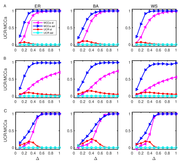
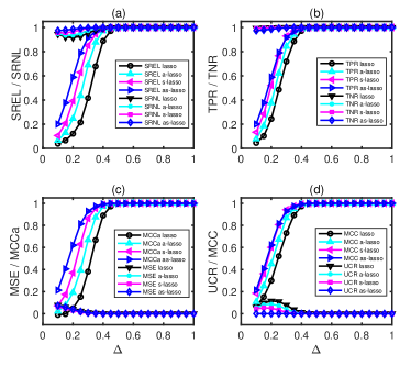
Fig. 3 plots the measures in Section III.4 against the data length in the PDG model with a small world (WS) network, using the methods of lasso, adaptive lasso, signal lasso, and adaptive signal lasso, where adaptive lasso represents one that performs best among the lasso-type methods and lasso is also included as a commonly used method (results for all methods are given in Supplemental Material and show that adaptive signal lasso performs best). It is clear that adaptive signal lasso performed best based on most measures, followed by signal lasso, adaptive lasso, and lasso. For measures TNR and MSE, adaptive signal lasso is not absolutely superior, but the differences of four methods are very small. It is of interest to see that UCR of adaptive signal lasso is close to zero even in the case of small , which is an appealing property.
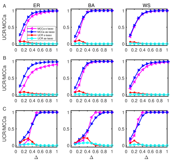
Fig. 4 A and B show the reconstruction accuracy measures of MCCa and UCR in the ER, WS, and BA networks respectively for in the PDG model when a noise is added to the model. We only list the results for signal lasso and adaptive signal lasso, since other methods performed more poorly than these two methods. Adaptive signal lasso is obviously superior to signal lasso when there is noise in the data, and UCR remains best (close to zero). For the large variance , adaptive signal lasso can still resist effect of noise according to Fig. 3, which indicates the robustness of adaptive signal lasso. Fig. 4C shows the results of a dense network with average degree equal to 20 and shows that adaptive signal lasso has higher values of MCCa than signal lasso at a small and approach being equal at a large , however, the UCR of adaptive signal lasso is always better than that of signal lasso.
IV.3 Kuramoto model in synchronization problem
For problems introduced in Eq. (2), we use the Kuramoto model Boccaletti et al. (2014); Timme (2007); Wu et al. (2012) to illustrate the reconstruction of the network in a complex system. This model has the following governing equation:
| (20) |
, where the system is composed of oscillators with phase and coupling strength , each of the oscillators has its own intrinsic natural frequency , is the adjacency matrix of a give network and is need to be estimated in network reconstruction. Using the same framework of referenceShi et al. (2021), the Euler method can be employed to generate time series with an equal time step . Let , , is a matrixShi et al. (2021), with elements
for and , , then reconstruction model can be written as
| (21) |
where denote a vector with all element 1.
Fig. 5 consider the Kuramoto model in ER, WS and BA networks respectively for and coupling strength . Panel A is the results without the noise, where we find the similar results as before analysis. Panel B is the result with variance of noise equal to 0.3, and it also show adaptive signal lasso method is robust against the noise. Panel C give the result of dense network with average degree 20, it is interest to observe that adaptive signal lasso performed better than signal lasso for small , while signal lasso become better than adaptive signal lasso for large , where UCR always performed well. This results implies that signal lasso is also useful in dense network, however adaptive signal lasso is more computationally convenient since it only need tuning one parameter.
V Examples
V.1 Human behavioral data
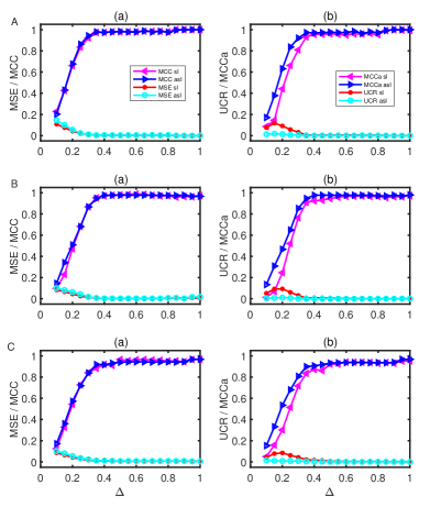
We use real data from a human behavior experiment, whose purpose is to study the impact of punishment on network reciprocity, to illustrate social network reconstruction Li et al. (2018). A total of 135 volunteers from Yunnan University of Finance and Economics and Tianjin University of Finance Economics participated in experiments with three trials. In treatment I, 35 participants played an iterative prisoner’s dilemma game with punishment on the static ring network with four neighbors. In treatments II and III, 50 participants participated in the same experiment, where treatment II was implemented on a homogeneous random network with degree 4, and in treatment III, each player was placed on a heterogeneous random network, where half the nodes had degree 3, and half had degree 5. The payoff matrices are presented in Table 3. Each player played with direct neighbors in each round to gain their payoff and updated the strategy to optimize their future payoff. The number of interactions in each session was 50, which was unknown to players. This dataset was analyzed to show that the signal lasso method outperformed the lasso and CS methods Shi et al. (2021); here we use this example again to study the performance of proposed method. The results are summarized in Fig. 6, where panels A, B, and C refer to the results of the experimental ring, homogeneous random, and heterogeneous random network, respectively. The figures in column (a) list the measures of MCC and MSE, and column (b) lists the measures of MCCa and UCR. It is clear that both for MCC and MCCa, adaptive signal lasso is superior to signal lasso, especially for MCCa. MSE of adaptive signal lasso is slightly larger than that of signal lasso for smaller values of . The UCR of adaptive signal lasso is close to zero for all values of , as expected, but UCR of signal lasso shows that it still contains some unclassified parts for smaller , which decreases reconstruction accuracy.
| C | D | P | |
|---|---|---|---|
| C | 2 | -2 | -5 |
| D | 4 | 0 | -3 |
| P | 2 | -2 | -5 |
| C | D | |
|---|---|---|
| C | 4 | -2 |
| D | 6 | 0 |
V.2 World Trade Web (WTW)
A network formed by import/export relationships between countries, the World Trade Web (WTW) has been extensively studied. Some empirical studies focused on the WTW as a complex network and investigated its architecture Squartini et al. (2011). When the available information on the system is incomplete or partial, reconstruction methods of the whole network have been proposed, such as maximum entropy Mistrulli (2011); Squartini et al. (2018) and the configuration model (CM) Garlaschelli and Loffredo (2004, 2009); Caldarelli et al. (2013). Much of the network reconstruction research in WTW focuses on ensemble models, which means that a model is defined to be not a single network, but a probability distribution over many possible networks Park and Newman (2004). We use a new perspective to illustrate the construction of a trade network using our proposed signal lasso method, which gives a model-based estimation of adjacency matrix A.
| Measures | lasso | A-lasso | S-lasso | AS-lasso |
|---|---|---|---|---|
| SREL | 0.0055 | 0.0202 | 0.9632 | 0.9710 |
| SRNL | 1 | 1 | 1 | 1 |
| TPR | 0.0075 | 0.0263 | 0.9652 | 0.9722 |
| TNR | 1 | 1 | 1 | 1 |
| MCC | 0.0246 | 0.0563 | 0.9659 | 0.9722 |
| MCCa | 0.0185 | 0.0446 | 0.9636 | 0.9282 |
| UCR | 0.2296 | 0.2038 | 0.0103 | 0.0022 |
| MSE | 1.3e+08 | 1.9e+03 | 0.266 | 0.1358 |
The database of the trade network is built from the data directly reported by each country to the United Nations Statistical Division, which is freely available from their website, which provides disaggregated data on bilateral trade flows for more than 5000 products and 200 countries from 1995 to 2018. Each trade flow is characterized by a combination of exporter-importer-products- year and provides the value and quantity of the flow. Because some countries do not report the values of their exports or imports, or because a large amount of data are missing, we only used data from 215 countries in the years 1995–2018, realizing a network of all trade products with 215 nodes and 36296 links, which is extremely dense Squartini et al. (2011).
We only considered an un-directional binary network, defining two countries as connected if one has output to another. Let denote total foreign trade (in U.S. dollars) of the th country, including total imports and exports with other countries. Let denote the import and export values of the th country with the th country at time . Then, it is obvious that
| (22) |
where is an element of a connectivity matrix with for , and is the number of countries. It is noted that for some country pairs, the export (or import) bilaterally or unilaterally at some time periods are missing, that means in some years during the observations there are no trade between two countries or missing because the trading quantity is small and can be ignored. Hence, the edges during 24 years might be incompletely linked, which is unbalanced.
In many economic network analyses and spatial panel data models, the adjacency matrix must be predetermined. A simple method to obtain an adjacency matrix is to define if there is a connection at least one time between two nodes, and otherwise Anselin (2013); Zhu et al. (2019). However, this may be unreasonable if two countries only have one year of very small or negligible trade. An alternative method is to use the percentage of the trade between two countries of the total trade amount to measure their connectivity, but they need a cutoff value, which might be subjective. An interesting problem is determining how to use the structural relationship, such as Eq. (22), to estimate the network during the observed periods; this problem can be dealt with using the shrinkage theory proposed in this paper since in this case is either 0 or 1. It is noted that the model in Eq. (22) relates to the reconstruction of binary topology, and we assume this is fixed during the observed time period, which is usually favorable in statistical network models Anselin (2013); Zhu et al. (2019).
For comparison, we define the reference connectivity as =1 if at least one connection occurs during the observed years, and zero otherwise. This is not assumed to be a correct adjacency matrix, but it can be used for comparison and analysis. The results are listed in Table 4, using as a baseline for comparison. It is surprising that lasso and adaptive lasso perform poorly in terms of SREL (TPR), MCC, MCCa, and MSE, even with high values of SRNL (TNR), perhaps because the trade network is highly dense, which was verified in our simulation of Section IV.1. The performance of signal lasso and adaptive signal lasso is excellent, and they give similar results. All methods can correctly identify non-existent links (SRNL and TPR have values of 1) because there are just a few zero edges (about 12%) in WTW. The values of SREL (TNR) of adaptive signal lasso can exceed 96%, even with .
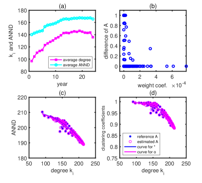
Fig. 7 shows some basic statistics calculated from the reference and estimated adjacency matrix. Fig. 7(a) shows the evolution of the average degree and average nearest neighbor degree (ANND) over the time calculated from , which shows that the trade network is time-dependent and has increasing degrees of nodes, but there is a downward trend in the last few years. Fig. 7(b) shows the absolute difference of reference adjacency matrix and estimated adjacency matrix (denoted by ) against their weight coefficients
The small value of means small imports/exports between two countries or few connections during 24 years. means inconsistent (consistent) results between and , and indicates the unclassified cases. It is clear that inconsistency only occurs at very small weight coefficients, and unclassified cases occur mostly at smaller weight coefficients. Further investigation finds that these two cases occur at , where is the number of years from 1995 to 2018 for which import/export statistics are available (namely nonzero). These results show that shrinkage estimation can eliminate unimportant linkages between nodes.
Fig. 7(c) and (d) show plots of average nearest neighbor degree (ANND) and clustering coefficients, respectively, versus average degree. We find the results from and are highly coincident, where decreasing trends have been found in previous studies employing different datasets in WTW Squartini et al. (2011). The decreasing trend in Fig. 7(c) is known as disassortativity (i.e., countries trading with highly connected countries have few trade partners, and those trading with poorly connected countries have many) in WTW Squartini et al. (2011).
VI Conclusions
We proposed adaptive signal lasso, based on the signal lasso method, to estimate signal parameters and uncover the topology in complex networks, adding a weight to penalty terms of signal lasso. The theoretical properties of this method were studied, and simulations were conducted, which included linear regression models, an evolutionary game dynamic model, and a simple synchronization model. Two real examples were analyzed. The results showed that our method can effectively uncover signals in network reconstruction in complex systems. Compared with signal lasso and other lasso-type methods, adaptive signal lasso has three advantages: (1) It only needs the tuning of one parameter in a small range in (0,1), which greatly reduces the computational cost; (2) Adaptive signal lasso is more robust to noise and contamination, as shown in the simulation of the PDG evolutionary model and Karumoto model, where adaptive signal lasso maintains good performance if the variance is not too large, while other methods fail; (3) Signal-type lasso, including signal lasso and adaptive signal lasso, outperforms other lasso-type methods, which is useful for the reconstruction of some non-sparse networks.
In the reconstruction of a WTW network, we used a simple example to illustrate our method, since a reference network is usually used in practice. We found our proposed method to be robust and efficient for both sparse and dense networks. When a directed network was considered, a similar analysis was conducted, and we also found that the signal-lasso-type method performed very well (see Supplemental Material). In practical situations, only partial information is available; e.g., we might only know in-degree or out-degree values in a binary network, in which case the problem can be solved by replacing in eq. (22) using an existing estimation method Squartini et al. (2018).
We only considered the detection of signal parameters (0 or 1) in binary networks. In weighted networks, the weight coefficient belongs to the interval [0,1] Squartini et al. (2018); Wang et al. (2011); Caldarelli et al. (2013). In such a circumstance, the proposed adaptive signal lasso can be applied by tuning the parameter in Eq. (11) to an appropriate value instead of letting it go to infinity (taking a large enough value as in our problem here). This topic will be studied in our future research.
Acknowledgement
This work was supported by NSFC under Grant No. 11931015, 12271471 to L. S. and JSPS Postdoctoral Fellowship Program for Foreign Researchers (No. P21374) and an accompanying Grant-in-Aid for Scientific Research to C. S.
Appendix
VI.1 Comparison of weight choice
If we assign the weight in both penalty terms, then and are two appropriate choices in adaptive signal lasso, where is the OLS estimator of . Fig. (8)(a) shows the curves of the penalty solution of adaptive signal lasso as a function of when , which is the formula used throughout this paper. Fig. (8)(b)–(d) show the solution of adaptive signal lasso as a function of in the three cases of and , and , and and , respectively. Although adaptive signal lasso in (b)–(d) also has the function of shrinking the values between 0 and 1 in two directions (0 or 1), it is too tedious and complicated, and sometime is unstable. Case (a), with and is the simplest but it can achieve our purpose very well. In addition, case (a) can reveal an appealing property (such as the result in Eq. 12) in selecting the tuning parameters in adaptive signal lasso, as we show in Eq. (12).
VI.2 The proof of Eq. (10) and (12)
In order to study the geometry of signal lasso, we assume that the columns of are orthogonal each other and . The ordinary least squares estimate in this special case then has the form of . Let , we then have
| (A.23) |
where and are known weight vectors and denotes the Hadamard production. Note that the first term is constant with respect to and . Using the fact that
| (A.24) |
and differentiating with respect to and set it to zero, after some calculations we have
| (A.25) |
in which is the solution of function . From our analysis in the main content of this paper, we choose that as adaptive lasso used and . When and , Eq. (10) can be derived easily from Eq. (A.25) .
Now we re-parameterize and by and , then we have
| (A.26) |
which will immediately lead to the results in Eq. (12).
VI.3 Coordinate descent algorithm
Differentiating (8) with respect to and equal it to zero, we have
| (A.27) |
where , ; sgn(z) takes values of sign(z) for and some value lying in for . Let denote the partial residual, where , then using formula (A.24) and after some calculation, we have
| (A.28) |
where denote the inner product of vectors and , and , and . From the definition of , it is easy to see
| (A.29) |
Note that , where , we have
| (A.30) |
Therefore the update can be written as
| (A.31) |
where denote the estimator of in the th step, and . The overall algorithm operates by applying this update repeatedly in a cyclical manner, updating the coordinates of along the way. Once an initial estimator of is given, for example by lasso estimation or ridge estimation, the update can be continued until convergence.
References
- Strogatz (2001) Steven H Strogatz, “Exploring complex networks,” Nature 410, 268 (2001).
- Barabási (2012) Barabási, “The network takeover,” Nat. Phys 8 (2012).
- Albert and Barabási (2002) Réka Albert and Albert-László Barabási, “Statistical mechanics of complex networks,” Reviews of Modern Physics 74, 47 (2002).
- Boccaletti et al. (2006) Stefano Boccaletti, Vito Latora, Yamir Moreno, Martin Chavez, and D-U Hwang, “Complex networks: Structure and dynamics,” Physics Reports 424, 175–308 (2006).
- Han et al. (2015) Xiao Han, Zhesi Shen, Wen-Xu Wang, and Zengru Di, “Robust reconstruction of complex networks from sparse data,” Physical Review Letters 114, 028701 (2015).
- Wang et al. (2011) Wen-Xu Wang, Ying-Cheng Lai, Celso Grebogi, and Jieping Ye, “Network reconstruction based on evolutionary-game data via compressive sensing,” Physical Review X 1, 021021 (2011).
- Peixoto (2018) Tiago P Peixoto, “Reconstructing networks with unknown and heterogeneous errors,” Physical Review X 8, 041011 (2018).
- Gardner et al. (2003) Timothy S Gardner, Diego Di Bernardo, David Lorenz, and James J Collins, “Inferring genetic networks and identifying compound mode of action via expression profiling,” Science 301, 102–105 (2003).
- Geier et al. (2007) Florian Geier, Jens Timmer, and Christian Fleck, “Reconstructing gene-regulatory networks from time series, knock-out data, and prior knowledge,” BMC Syst. Biol 1 (2007).
- Grün et al. (2002) Sonja Grün, Markus Diesmann, and Ad Aertsen, “Unitary events in multiple single-neuron activity. i. detection and significance,” Neural Comput. 14 (2002).
- Supekar et al. (2008) Kaustubh Supekar, Vinod Menon, Daniel Rubin, Mark Musen, and Michael D Greicius, “Network analysis of intrinsic functional brain connectivity in alzheimer’s disease,” PLoS Comput Biol 4, e1000100 (2008).
- Squartini et al. (2018) Tiziano Squartini, Guido Caldarelli, Giulio Cimini, Gabrielli Andrea, and Diego Garlaschelli, “Reconstruction methods for networks: the case of economic and financial systems,” Physics Reports 757, 1–14 (2018).
- Shi et al. (2020a) Lei Shi, Chen Shen, Qi Shi, Zhen Wang, Jianhua Zhao, Xuelong Li, and Stefano Boccaletti, “Recovering network structures based on evolutionary game dynamics via secure dimensional reduction,” IEEE Transactions on Network Science and Engineering 7, 2027–2036 (2020a).
- Shi et al. (2021) Lei Shi, Chen Shen, Libin Jin, Qi Shi, Zhen Wang, and Boccaletti Stefano, “Inferring network structures via signal lasso,” Physical Review Research 3, 043210 (2021).
- Wang et al. (2016) Wen-Xu Wang, Ying-Cheng Lai, and Celso Grebogi, “Data based identification and prediction of nonlinear and complex dynamical systems,” Physics Reports 644, 1–76 (2016).
- Raimondo and Domenico (2021) Sebastian Raimondo and Manlio De Domenico, “Measuring topological descriptors of complex networks under uncertainty,” Physical Review E 103, 022311 (2021).
- Santos and Pacheco (2005) Francisco C Santos and Jorge M Pacheco, “Scale-free networks provide a unifying framework for the emergence of cooperation,” Physical Review Letters 95, 098104 (2005).
- Nowak and May (1992) Martin A Nowak and Robert M May, “Evolutionary games and spatial chaos,” Nature 359, 826 (1992).
- Hauert and Doebeli (2004) Christoph Hauert and Michael Doebeli, “Spatial structure often inhibits the evolution of cooperation in the snowdrift game,” Nature 428, 643 (2004).
- Szabó and Fath (2007) György Szabó and Gabor Fath, “Evolutionary games on graphs,” Physics reports 446, 97–216 (2007).
- Perc et al. (2017) Matjaž Perc, Jillian J Jordan, David G Rand, Zhen Wang, Stefano Boccaletti, and Attila Szolnoki, “Statistical physics of human cooperation,” Physics Reports 687, 1–51 (2017).
- Li et al. (2018) Xuelong Li, Marko Jusup, Zhen Wang, Huijia Li, Lei Shi, Boris Podobnik, H Eugene Stanley, Shlomo Havlin, and Stefano Boccaletti, “Punishment diminishes the benefits of network reciprocity in social dilemma experiments,” Proceedings of the National Academy of Sciences 115, 30–35 (2018).
- Wang et al. (2017) Zhen Wang, Marko Jusup, Rui-Wu Wang, Lei Shi, Yoh Iwasa, Yamir Moreno, and Jürgen Kurths, “Onymity promotes cooperation in social dilemma experiments,” Science advances 3, e1601444 (2017).
- Wang et al. (2018) Zhen Wang, Marko Jusup, Lei Shi, Joung-Hun Lee, Yoh Iwasa, and Stefano Boccaletti, “Exploiting a cognitive bias promotes cooperation in social dilemma experiments,” Nature communications 9, 2954 (2018).
- Shi et al. (2020b) Lei Shi, Ivan Romić, Yongjuan Ma, Zhen Wang, Boris Podobnik, H Eugene Stanley, Peter Holme, and Marko Jusup, “Freedom of choice adds value to public goods,” Proceedings of the National Academy of Sciences 117, 17516–175211 (2020b).
- Szabó et al. (2005) György Szabó, Jeromos Vukov, and Attila Szolnoki, “Phase diagrams for an evolutionary prisoner’s dilemma game on two-dimensional lattices,” Physical Review E 72, 047107 (2005).
- Tibshirani (1996) Robert Tibshirani, “Regression shrinkage and selection via the lasso,” Journal of the Royal Statistical Society: Series B (Methodological) 58, 267–288 (1996).
- Hastie et al. (2015) Trevor Hastie, Robert Tibshirani, and Martin Wainwright, Statistical learning with sparsity: the lasso and generalizations (CRC press, 2015).
- Marbach et al. (2012) Daniel Marbach, James C Costello, Robert Küffner, Nicole M Vega, Robert J Prill, Diogo M Camacho, Kyle R Allison, The DREAM5 Consortium, Manolis Kellis, James J Collins, and Gustavo Stolovitzky, “Wisdom of crowds for robust gene network inference,” Nature Methods 9, 796–804 (2012).
- Chicco (2017) Davide Chicco, “Ten quick tips for machine learning in computational biology,” BioData Mining 10 (2017).
- Chicco and Jurman (2020) Davide Chicco and Giuseppe Jurman, “The advantages of the matthews correlation coefficient (mcc) over f1 score and accuracy in binary classification evaluation,” BMC genomics 21, 1–13 (2020).
- Fan et al. (2009) Jianqing Fan, Yang Feng, and Yichao Wu, “Network exploration via the adaptive lasso and scad penalties,” The Annals of Applied Statistics 3, 521 (2009).
- Fan and Li (2001) Jianqing Fan and Runze Li, “Variable selection via nonconcave penalized likelihood and its oracle properties,” Journal of the American statistical Association 96, 1348–1360 (2001).
- Szabó and Tőke (1998) György Szabó and Csaba Tőke, “Evolutionary prisoner’s dilemma game on a square lattice,” Physical Review E 58, 69 (1998).
- Szabó and Hauert (2002) György Szabó and Christoph Hauert, “Evolutionary prisoner’s dilemma games with voluntary participation,” Physical Review E 66, 062903 (2002).
- Boccaletti et al. (2014) Stefano Boccaletti, Ginestra Bianconi, Regino Criado, Charo I Del Genio, Jesús Gómez-Gardenes, Miguel Romance, Irene Sendina-Nadal, Zhen Wang, and Massimiliano Zanin, “The structure and dynamics of multilayer networks,” Physics Reports 544, 1–122 (2014).
- Timme (2007) Marc Timme, “Revealing network connectivity from response dynamics,” Physical Review Letters 98, 224101 (2007).
- Wu et al. (2012) Xiaoqun Wu, Weihan Wang, and Wei Xing Zheng, “Inferring topologies of complex networks with hidden variables,” Physical Review E 86, 046106 (2012).
- Squartini et al. (2011) Tiziano Squartini, Giorgio Fagiolo, and Diego Garlaschelli, “Randomizing world trade. ii. a weighted network analysis,” Physical Review E 84 (2011).
- Mistrulli (2011) Paolo Emilio Mistrulli, “Assessing financial contagion in the interbank market: Maximum entropy versus observed interbank lending patterns,” J. Bank. Finance 35, 1114–1127 (2011).
- Garlaschelli and Loffredo (2004) Diego Garlaschelli and Maria I. Loffredo, “Fitness dependent topological properties of the world trade web,” Phys. Rev. Lett. 93 (2004).
- Garlaschelli and Loffredo (2009) Diego Garlaschelli and Maria I. Loffredo, “Generalized bose- fermi statistics and structural correlations in weighted networks,” Phys. Rev. Lett. 102 (2009).
- Caldarelli et al. (2013) Guido Caldarelli, Alessandro Chessa, Gabrielli Andrea, Fabio Pammolli, and Michelangelo Puliga, “Reconstructing a credit network,” Nature Physics 9 (2013).
- Park and Newman (2004) Juyong Park and Mark EJ Newman, “The statistical mechanics of networks,” Phys. Rev. E 70 (2004).
- Anselin (2013) Luc Anselin, “Spatial econometrics: Method and models,” Springer Science & Business Media 4 (2013).
- Zhu et al. (2019) Xuening Zhu, Weining Wang, Hansheng Wang, and Wolfgang Karl Härdle, “Network quantile autoregression,” Journal of econometrics 212, 345–358 (2019).