ZigZag: Universal Sampling-free Uncertainty
Estimation Through Two-Step Inference

Abstract

Whereas the ability of deep networks to produce useful predictions has been amply demonstrated, estimating the reliability of these predictions remains challenging. Sampling approaches such as MC-Dropout and Deep Ensembles have emerged as the most popular ones for this purpose. Unfortunately, they require many forward passes at inference time, which slows them down. Sampling-free approaches can be faster but suffer from other drawbacks, such as lower reliability of uncertainty estimates, difficulty of use, and limited applicability to different types of tasks and data.

In this work, we introduce a sampling-free approach that is generic and easy to deploy, while producing reliable uncertainty estimates on par with state-of-the-art methods at a significantly lower computational cost. It is predicated on training the network to produce the same output with and without additional information about it. At inference time, when no prior information is given, we use the network’s own prediction as the additional information. We then take the distance between the predictions with and without prior information as our uncertainty measure.

We demonstrate our approach on several classification and regression tasks. We show that it delivers results on par with those of Ensembles but at a much lower computational cost.

Introduction

Though the ability of modern neural networks to generate accurate predictions is now clear, assessing the trustworthiness of these predictions remains an open problem. This can be addressed by estimating the potential inaccuracy of the predictions, which is then taken as an uncertainty measure. MC-Dropout (Gal and Ghahramani 2016) and Deep Ensembles (Lakshminarayanan, Pritzel, and Blundell 2017) are the most widely methods used to this end. MC-Dropout involves randomly zeroing out network weights and assessing the effect, whereas Ensembles involves training multiple networks, starting from different initial conditions. They are simple to deploy and universal. Unfortunately, they induce substantial computational and memory overheads, which makes them unsuitable for many real-world applications.

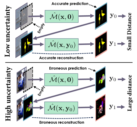
Figure 1: ZigZaging. At inference time, we make two forward passes. First, we use $[\mathbf{x},\textbf{0}]$ as input to produce a prediction $\mathbf{y}_{0}$. Second, we feed $[\mathbf{x},\mathbf{y}_{0}]$ to the network and generate $\mathbf{y}_{1}$. We take $\|\mathbf{y}_{0}-\mathbf{y}_{1}\|$ to be our uncertainty estimate.

An alternative is to use sampling-free methods that estimate uncertainty in one single forward pass of a single neural network, thereby avoiding computational overheads (Amersfoort et al. 2020; Malinin and Gales 2018; Tagasovska and Lopez-Paz 2018; Postels et al. 2019). However, deploying them usually requires heavily modifying the network’s architecture (Postels et al. 2019), significantly changing the training procedures (Malinin and Gales 2018), or limiting oneself to very specific tasks (Amersfoort et al. 2020; Malinin and Gales 2018; Mukhoti et al. 2021b). As a result, they have not gained as much traction as MC-Dropout and Ensembles.

To remedy this, we introduce ZigZag, a sampling-free approach that is generic and easy to deploy, while producing reliable uncertainty estimates on par with sampling-based methods at a significantly lower computational cost. It relies on making a first prediction and then checking its accuracy by making a second one based on the first. To make this effective, we train the network so that, if the first prediction is correct, the second also is. Thus, a large discrepancy between the two predictions signals potential inaccuracy.

In practice, given a network $\mathcal{M}$, we modify its first layer to accept a second argument, yielding the modified architecture $\hat{\mathcal{M}}$. We then train $\hat{\mathcal{M}}$ so that, for all training pairs $(\mathbf{x},\mathbf{y})$, we have $\mathbf{y}\approx\hat{\mathcal{M}}(\mathbf{x},\mathbf{0})\approx\hat{\mathcal{M}}(\mathbf{x},\mathbf{y})$, where $\mathbf{0}$ is a vector of zeros. At inference time, we first compute $\hat{\mathcal{M}}(\mathbf{x},\mathbf{0})$ and then $\hat{\mathcal{M}}(\mathbf{x},\hat{\mathcal{M}}(\mathbf{x},\mathbf{0}))$. We refer to this as ZigZagging, as depicted by Fig. 1. Finally, we take the distance between the two predictions $\|\hat{\mathcal{M}}(\mathbf{x},\mathbf{0})-\hat{\mathcal{M}}(\mathbf{x},\hat{\mathcal{M}}(\mathbf{x},\mathbf{0}))\|$ as our error estimate. This exploits the fact that, if $\hat{\mathcal{M}}(\mathbf{x},\mathbf{0})$ is accurate, that is, $\hat{\mathcal{M}}(\mathbf{x},\mathbf{0})\approx\mathbf{y}$, then the second prediction should be similar to the first because of the way the network has been trained. Otherwise, we have an indication that something is wrong with $\hat{\mathcal{M}}(\mathbf{x},\mathbf{0})$. Furthermore, in our training scheme, an input/output pair $(\mathbf{x},\mathbf{y})$ is in-distribution if $\mathbf{y}$ is either the ground-truth target or $\mathbf{0}$ and out-of-distribution otherwise, which is the case at inference time if $\hat{\mathcal{M}}(\mathbf{x},\mathbf{0})$ is wrong. As networks often deliver random answers for out of distribution samples, $\|\hat{\mathcal{M}}(\mathbf{x},\mathbf{0})-\hat{\mathcal{M}}(\mathbf{x},\hat{\mathcal{M}}(\mathbf{x},\mathbf{0}))\|$ tends to be large in that situation. We validate this behavior experimentally.

Our approach is fast because it only requires performing two forward passes using one single network and delivers uncertainty results comparable to those of Ensembles, which are much more costly but often seen as the method that delivers the best uncertainty estimates on a wide range of classification and regression problems. Furthermore, it is very easy to use in conjunction with almost any network architecture with only very minor changes. Hence, our method is also task-agnostic.

Related work

Uncertainty Estimation (UE) aims to accurately evaluate the reliability of a model’s predictions. Among all the methods that can be used to do this, MC-Dropout (Gal and Ghahramani 2016) and Deep Ensembles (Lakshminarayanan, Pritzel, and Blundell 2017) have emerged as two of the most popular ones, with Bayesian Networks (Mackay 1995) being a third alternative. These methods are sampling-based and require several predictions at inference time, which slows them down. There is recent work on overcoming this and we discuss both kinds of approaches below.

Sampling-based Approaches.

MC-Dropout involves randomly zeroing out network weights and assessing the effect, whereas Ensembles involve training multiple networks, starting from different initial conditions. The extensive survey of (Ashukha et al. 2020) concludes that Deep Ensembles tend to produce the most decorrelated models, which results in highly diversified predictions and the most reliable uncertainty estimates. Unfortunately, Deep Ensembles also entail the highest computation costs due to the need to train multiple networks and to run up to dozens of forward passes at inference time. MC-Dropout tends to be less reliable and also involves making several inferences at inference time. There have been recent attempts at increasing the reliability of MC-Dropout (Durasov et al. 2021a; Weller and Jebara 2014) but they do not address the fact that multiple inferences are required to estimate the uncertainty. Alternative sampling-based methods such as (Mi et al. 2022) rely on noise injections or input augmentations during inference in order to produce uncertainty from the variance of generated predictions. Bayesian Networks (Blundell et al. 2015; Graves 2011; Hernández-Lobato and Adams 2015; Kingma, Salimans, and Welling 2015) also require several forward passes to compute uncertainty and rarely outperform Deep Ensembles (Ashukha et al. 2020). In short, for sampling-based methods, computation time scales linearly with the number of samples and can be prohibitively expensive for performance-critical applications.

Sampling-free Approaches.

When a rapid response is needed, for example for robotic control (Loquercio, Segu, and Scaramuzza 2020) or low-latency (Gal 2016) applications, there is no time to perform many forward passes during inference. Consequently, there has been much interest for sampling-free approaches that require constant time for inference. For example, in (Amersfoort et al. 2020), a clustering-like procedure is used to estimate uncertainty for classification and semantic segmentation purposes. In (Malinin and Gales 2018; Malinin et al. 2020), uncertainty is estimated from Dirichlet and Normal-Wishart distributions whose parameters are predicted by the network. Unfortunately, there rarely is a clear way to extend these mostly classification approaches to regression. Furthermore, deploying them often requires significantly changing the network architecture and the training procedures (Liu et al. 2020; Shekhovtsov and Flach 2019; Wannenwetsch and Roth 2020), along with increased memory consumption (Wang, Shi, and Yeung 2016; Shekhovtsov and Flach 2019; Gast and Roth 2018), worse uncertainty quality (Tagasovska and Lopez-Paz 2018; Mukhoti et al. 2021a) or slower inference (Postels et al. 2019), which limits their appeal.

Regression is handled in (Postels et al. 2019; Gast and Roth 2018) using an uncertainty estimation method that relies on uncertainty propagation from one layer to another. During the forward pass, not only activations but also their variances are estimated in each layer. Thus, the variance of the final predictions can be estimated in one pass but at the cost of a two-fold memory consumption and we will show that our approach performs better. In (Tagasovska and Lopez-Paz 2018), both quantile regression (Furno and Vistocco 2018) and orthonormal certificates are used to detect out-of-distribution samples during inference. Though being computationally efficient, this approach also can yield poor uncertainty estimates and miscalibrated predictions. SNGP (Liu et al. 2020) has been used to estimate uncertainty in a deep learning context, but this requires adding a Random Features (Rahimi and Recht 2007) and Spectral Normalization (Miyato et al. 2018) layer to every convolutional layer, which entails significant modifications of both training dynamic and network architectures. Similarly, the approaches of (Wang, Shi, and Yeung 2016; Shekhovtsov and Flach 2019) require replacing all of the convolution layers with modified versions and to double the number of weights, which significantly impacts memory consumption. Other types of methods such as (Zhang et al. 2019) work only with specific uncertainty types, either aleatoric or epistemic (Der Kiureghian and Ditlevsen 2009; Kendall and Gal 2017). Furthermore, in some cases, they can yield significantly worse uncertainty calibration than sampling-based approaches (Postels et al. 2021). We provide more specific comparisons in the experiment section.

Method

ZigZag is an approach to sampling-free uncertainty estimation that delivers classification and regression results on par with state-of-the-art sampling-based methods such as Ensembles and MC-Dropout while being far less computationally demanding. It relies on the dual-inference scheme depicted by Fig. 1. Given a network $\hat{\mathcal{M}}$ and a sample x, we first use $\hat{\mathcal{M}}$ to make a first prediction $\mathbf{y}_{0}$ without any prior information. We then make a second prediction $\mathbf{y}_{1}$ using $\mathbf{y}_{0}$ as a prior. We train the network so that, if $\mathbf{y}_{0}$ is correct, then $\mathbf{y}_{1}$ should be similar to $\mathbf{y}_{0}$, whereas it should be different if $\mathbf{y}_{0}$ is inaccurate. In the remainder of this section, we describe how we achieve this goal.

Modifying the Original Architecture

Let $\mathcal{M}$ be a network that takes as input a vector $\mathbf{x}$ and returns a prediction vector $\mathcal{M}(\mathbf{x})$ that should be close to target $\mathbf{y}$. We modify the first layer of $\mathcal{M}$ to create a new architecture $\hat{\mathcal{M}}$ that takes as input both $\mathbf{x}$ and a vector of the same dimension as $\mathbf{y}$ so that we can compute both $\hat{\mathcal{M}}(\mathbf{x},\mathbf{0})$ and $\hat{\mathcal{M}}(\mathbf{x},\mathbf{y})$, where $\mathbf{0}$ is a vector of zeros of the same dimension as $\mathbf{y}$. We take $\hat{\mathcal{M}}(\mathbf{x},\mathbf{0})$ to be the prediction without prior information and $\hat{\mathcal{M}}(\mathbf{x},\mathbf{y})$ one with prior information. In practice, $\mathcal{M}$ can be any sufficiently powerful deep architecture, such as VGG (Simonyan, Vedaldi, and Zisserman 2014), ResNet (He et al. 2016) or a Transformer (Dosovitskiy et al. 2020). In all these cases, modifying the first network layer is a simple task.

For simplicity, let us first consider the case where $\mathcal{M}$ is a simple network with one hidden layer of dimension $h$. It takes $\mathbf{x}\in\mathbb{R}^{d}$ as input and outputs a scalar $y\in\mathbb{R}$. To handle a second argument $\mathbf{y}$, the input dimension of the first trainable layer must become $d+1$ to allow the concatenation of the original input vector $\mathbf{x}$ and the additional value $\mathbf{y}$. Similarly, we can add additional channels to convolutional layers to work with RGB images, for example by adding a fourth channel that represents $\mathbf{y}$. As before, we only need to modify the first convolutional layer of the network so that it can process 4-dimensional inputs.

Training

At the heart of our approach is the training of $\hat{\mathcal{M}}$ to yield comparable outputs, whether or not the target $\mathbf{y}$ is provided as input. In practice, we want $\hat{\mathcal{M}}(\mathbf{x},\mathbf{0})\approx\hat{\mathcal{M}}(\mathbf{x},\mathbf{y})\approx\mathbf{y}$ for all training pairs $(\mathbf{x},\mathbf{y})$. To this end, given a training pair$(\mathbf{x},\mathbf{y})$, we consider the loss

$$\mathcal{L}(\hat{\mathcal{M}}(\mathbf{x},\mathbf{0}),\mathbf{y})+\mathcal{L}(\hat{\mathcal{M}}(\mathbf{x},\mathbf{y}),\mathbf{y})\;,$$ (1)

where $\mathcal{L}$ is a domain-dependent loss term whose minimization ensures that the prediction made by $\mathcal{M}$ is close to the target $\mathbf{y}$. By minimizing this loss for all samples, we guarantee that our model can make accurate predictions when provided either with $\mathbf{0}$, that is, no prior information, or with accurate prior information in the form of the full answer $\mathbf{y}$.

Inference

At inference time, we compute

$$\hat{\mathbf{y}}=\mathbf{y}_{0}=\hat{\mathcal{M}}(\mathbf{x},\mathbf{0})\;,$$ (2)

$$\mathbf{y}_{1}=\hat{\mathcal{M}}(\mathbf{x},\mathbf{y}_{0})=\hat{\mathcal{M}}(\mathbf{x},\hat{\mathcal{M}}(\mathbf{x},\mathbf{0}))\;,$$

$$\hat{\mathbf{u}}=\|\mathbf{y}_{0}-\mathbf{y}_{1}\|\;,$$ (3)

where $\hat{\mathbf{y}}$ is our final prediction and $\hat{\mathbf{u}}$ our uncertainty estimate. $\mathbf{y}_{0}$ is estimated without prior information, whereas $\mathbf{y}_{1}$ is computed by using $\mathbf{y}_{0}$ as the prior information. If $\mathbf{y}_{0}$ is accurate, providing it as prior information should not disturb the inference because $\hat{\mathcal{M}}$ has been trained to return the correct answer when given the correct answer as prior information. This should result in $\mathbf{y}_{1}$ being similar to $\mathbf{y}_{0}$ and a small $\hat{\mathbf{u}}$. Consequently a large $\hat{\mathbf{u}}$ is an indication that supplying $\mathbf{y}_{0}$ as the prior information has disrupted the inference mechanism and that $\mathbf{y}_{0}$ is probably inaccurate.

This can also be understood in terms of the well-known tendency of networks to return arbitrary answers for samples that are out-of-distribution (OOD) with respect to the data they were trained on (Zhang et al. 2021; Lakshminarayanan, Pritzel, and Blundell 2017; Nguyen, Yosinski, and Clune 2015). The training scheme introduced above is such that the in-distribution training pairs are of the form $(\mathbf{x},\mathbf{z})$, where $\mathbf{z}$ is either $\mathbf{0}$ or the ground-truth $\mathbf{y}$. When $\mathbf{y}_{0}$ is inaccurate and we use it to compute $\mathbf{y}_{1}=\hat{\mathcal{M}}(\mathbf{x},\mathbf{y}_{0})$, we are essentially feeding an OOD sample to the network and the result $\mathbf{y}_{1}$ can be expected to be random, and therefore very different in general of $\mathbf{y}_{0}$. Our experiments on validation data bear this out, as shown in Fig. 2.

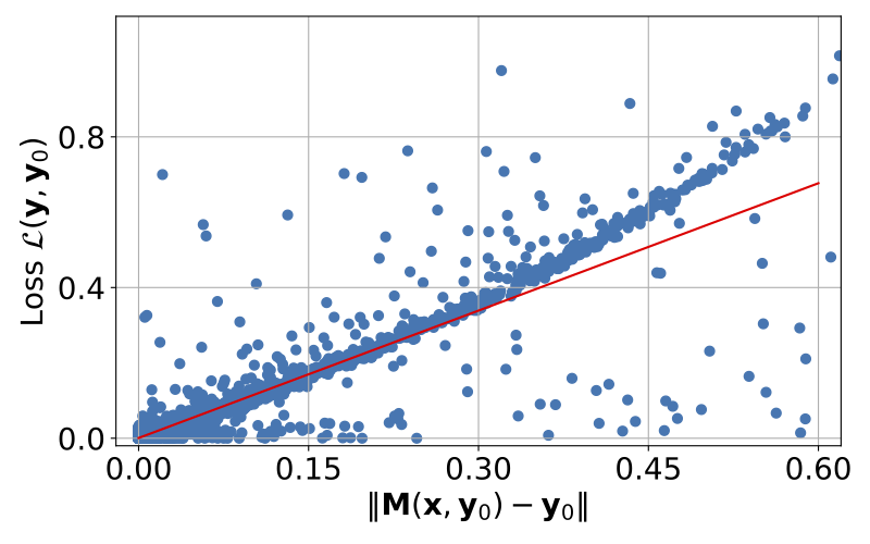
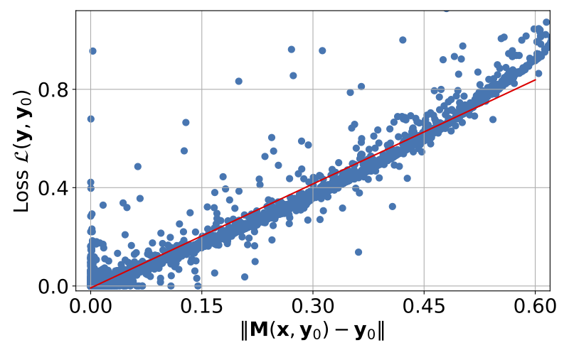
Figure 2: True vs Estimated Error. We use MNIST (left) and CIFAR (right) validation data to plot the true prediction errors as measured by the loss being minimized against our uncertainty estimates $\|\hat{\mathcal{M}}(\mathbf{x},\mathbf{0})-\hat{\mathcal{M}}(\mathbf{x},\hat{\mathcal{M}}(\mathbf{x},\mathbf{0}))\|$ for individual samples. In both cases, the correlation is strong and Pearson’s correlation coefficient is above 90%. The red line represents a linear fit to the data.

Experiments

We first introduce our metrics and baselines. We then use simple synthetic data to illustrate the behavior of ZigZag. Next, we turn to image datasets often used to test uncertainty-estimation algorithms. Finally, we present real-world applications. Implementation details about the baselines, metrics, training setups, and hyper-parameters could be found in the supplementary material.

Metrics and Baselines

We now introduce the evaluation metrics we use to quantitatively compare our methods against several baselines.

Accuracy Metric.

For classification tasks, we use the standard classification accuracy, i.e. the percentage of correctly classified samples in the test set. For regression tasks, we use the standard Mean Absolute Error (MAE) metric.

Uncertainty Metrics.

As in (Postels et al. 2021), we use Relative Area Under the Lift Curve (rAULC) to quantify the quality of calibration of uncertainty measures both for classification and regression tasks. Unlike other metrics (Brier et al. 1950; Guo et al. 2017), it is suitable for sampling-free approaches to estimate uncertainty.

Another way to estimate how good uncertainty estimates are is to use them to detect out-of-distribution samples under the assumption that the network is more uncertain about those than about samples from the distribution used to train it. As in (Malinin and Gales 2018; Durasov et al. 2021a), given both in- and out-of-distribution (OOD) samples, we classify high-uncertainty ones as OOD and rely on standard classification metrics, ROC and PR AUCs, to quantify the classification performance.

Time, Memory, and Simplicity.

The Time and Size metrics measure how much time and memory it takes to train the network(s) to estimate uncertainty, compared to a single one that does not estimate it. The Simplicity metric assesses how easy it is to modify a given architecture to obtain uncertainty estimates. We denote it as simple (✓) if it requires changing less than $10\%$ of layers of the original model and the training procedures do not need to be substantially modified. We also report Inference Time that represents how much time the model takes to compute uncertainties relative to single model inference on Tesla V100 and without considering parallelization for sampling-based approaches.

Baselines.

We compare against recent sample-based approaches—MC-Dropout (Gal and Ghahramani 2016) (MC-D), Deep Ensembles (Lakshminarayanan, Pritzel, and Blundell 2017) (DeepE), BatchEnsemble (Wen, Tran, and Ba 2020) (BatchE) and Masksembles (Durasov et al. 2021a) (MaskE) —and sample-free ones—-Single Model (Kendall and Gal 2017) (Single), Orthonormal Certificates (Tagasovska and Lopez-Paz 2019) (OC), SNGP (Liu et al. 2020) (SNGP), Variance Propagation (Postels et al. 2019) (VarProp). For all four sampling-based approaches, we use five samples to estimate the uncertainty at inference time. This number of samples has been shown to perform well for many tasks (Durasov et al. 2021a; Wen, Tran, and Ba 2020; Malinin and Gales 2018). All of the training and implementation details are provided in supplementary material.

Simple Synthetic Data.

We use such data to illustrate how ZigZag behaves both for classification and regression.

Classification Task.

Let us consider the red and blue 2D points shown in Fig. 3. We use them to train an MLP with 6 fully-connected layers and LeakyReLU activations to classify other points in the plane as belonging either to the red or the blue class. The background color in each of the subplots depicts the uncertainty estimated by Single-Model, MC-Dropout, Deep Ensembles, and ZigZag. The first two only exhibit uncertainty along a narrow band between the two distributions. This is highly questionable once one is far away from the data points in the lower left and upper right corners of the range. Both Ensembles and ZigZag deliver more plausible high uncertainties once far from the training points, but ZigZag does it at a lower computational cost.

Regression Task.

	MC-D	DeepE	BatchE	MaskE	Single	OC	SNGP	VarProp	ZigZag
Accuracy ($\uparrow$)	0.981	0.990	0.989	0.989	0.980	0.980	0.984	0.986	0.982	MNIST
rAULC ($\uparrow$)	0.932	0.958	0.941	0.929	0.712	0.851	0.813	0.731	0.961
Size	1x	5x	1.2x	1x	1x	1.3x	1x	1x	1x
Inf. Time	5x	5x	5x	5x	1x	1.4x	1.7x	1.2x	2x
Time	1.3x	5x	1.4x	1.3x	1x	1.1x	1.1x	1.x	1x
ROC-AUC ($\uparrow$)	0.953	0.984	0.965	0.963	0.773	0.934	0.951	0.812	0.982
PR-AUC ($\uparrow$)	0.962	0.979	0.965	0.966	0.844	0.923	0.942	0.861	0.981
Accuracy ($\uparrow$)	0.909	0.929	0.911	0.901	0.8901	0.892	0.905	0.895	0.928	CIFAR
rAULC ($\uparrow$)	0.889	0.911	0.884	0.889	0.884	0.583	0.742	0.715	0.897
Size	1x	5x	1.2x	1x	1x	1x	1x	1x	1x
Inf. Time	5x	5x	5x	5x	1x	1.1x	1.1x	1.2x	2x
Time	1.2x	5x	1.4x	1.3x	1x	1.3x	1x	1.2x	1.2x
ROC-AUC ($\uparrow$)	0.854	0.915	0.877	0.900	0.825	0.851	0.900	0.831	0.901
PR-AUC ($\uparrow$)	0.918	0.949	0.919	0.931	0.8747	0.821	0.891	0.861	0.933
Accuracy ($\uparrow$)	0.74	0.77	0.73	0.74	0.75	0.75	0.74	0.73	0.75	ImageNet
rAULC ($\uparrow$)	0.78	0.84	0.78	0.79	0.80	0.71	0.8	0.69	0.82
Size	1x	5x	1.1x	1.1x	1x	1x	1x	1x	1x
Inf. Time	5x	5x	5x	5x	1x	1.1x	1x	1x	2x
Time	1x	5x	1.1x	1x	1x	1x	1x	1.1x	1.3x
ROC-AUC ($\uparrow$)	0.52	0.56	0.53	0.52	0.51	0.52	0.53	0.50	0.54
PR-AUC ($\uparrow$)	0.16	0.19	0.16	0.14	0.15	0.17	0.13	0.12	0.17
Simple	✓	✓	✗	✗	-	✓	✗	✗	✓

Table 1: Classification results on MNIST (top), CIFAR (middle), and ImageNet (bottom). The best result in each category is in bold and the second best is in bold. Most correspond to ZigZag and DeepE. Hence, they perform similarly but ZigZag requires far less computation and memory.

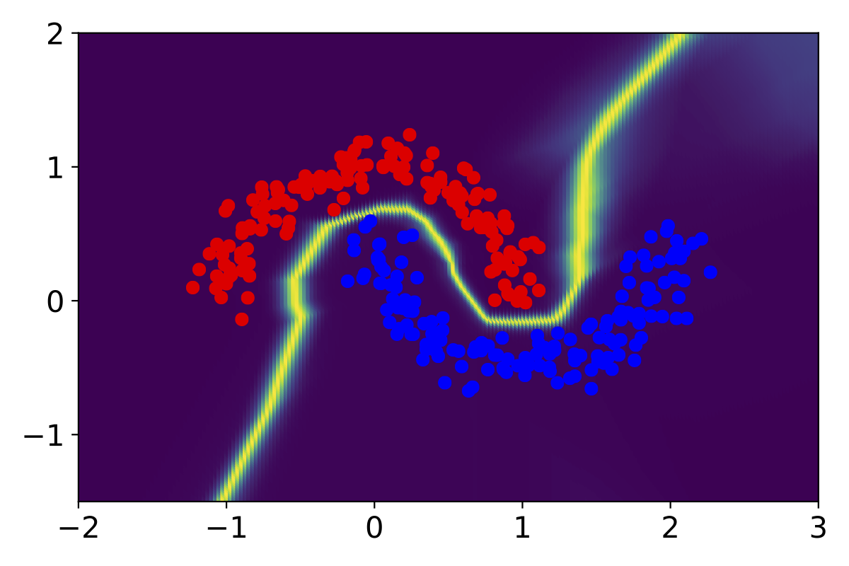
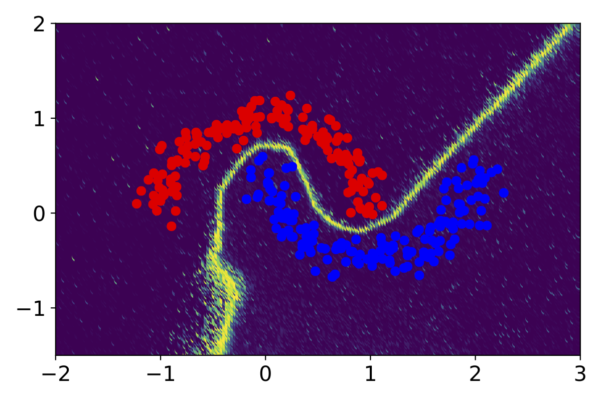
(a)	(b)
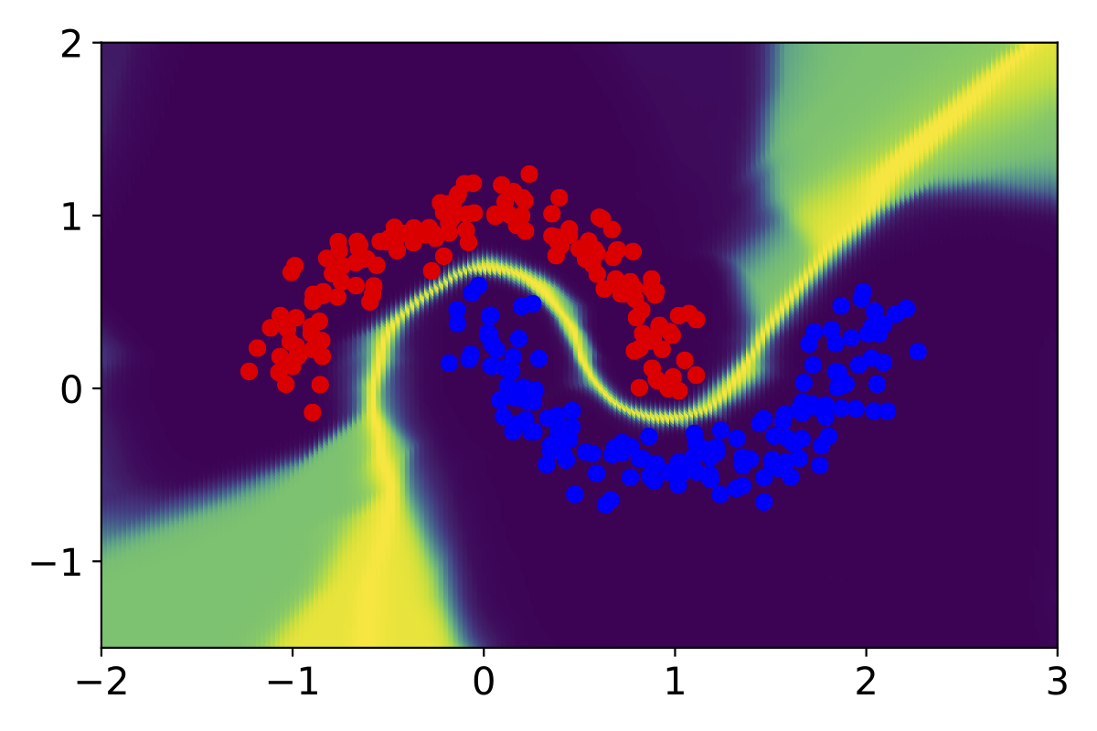
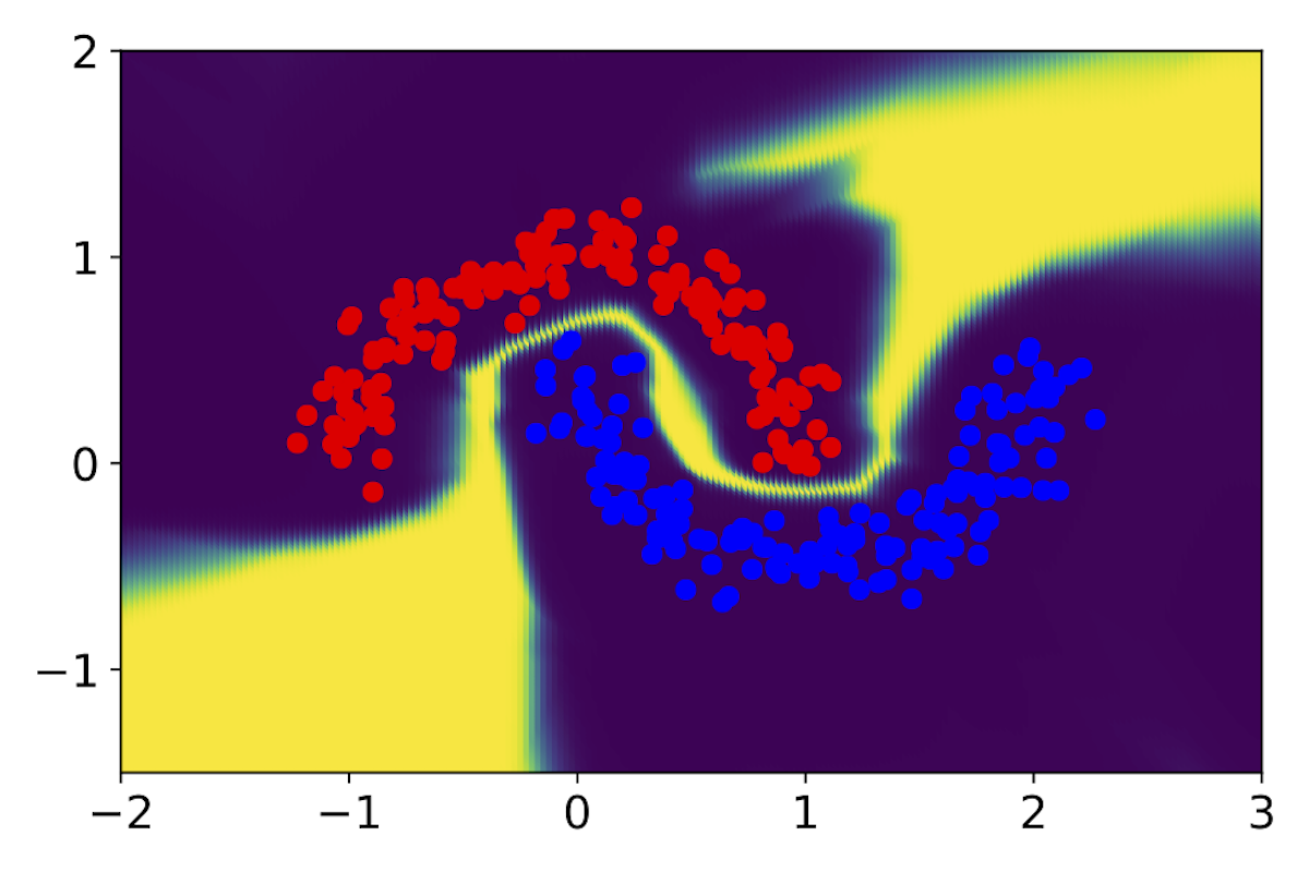
(c)	(d)

Figure 3: Uncertainty Estimation for Classification. The task is to classify data points drawn in the range $x\in[-2,3]$, $y\in[-2,2]$ as being red or blue given the red and blue training samples from two interleaving half circles with added Gaussian noise. The background color depicts the classification uncertainty assigned by different techniques to individual grid points. Violet is low and yellow is high. (a) Single model, (b) MC-Dropout, (c) Deep Ensembles, (d) ZigZag.

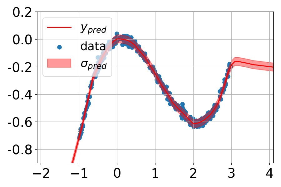
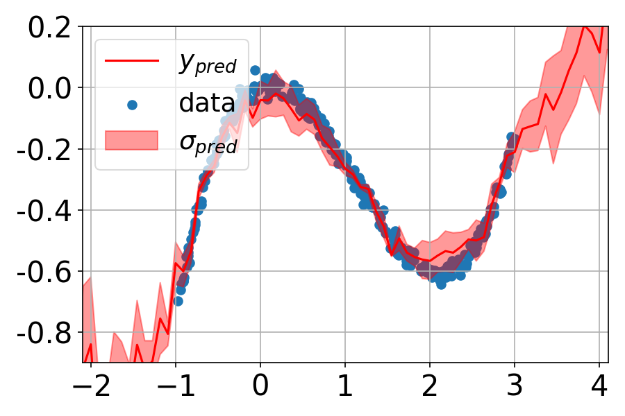
(a)	(b)
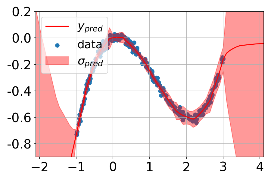
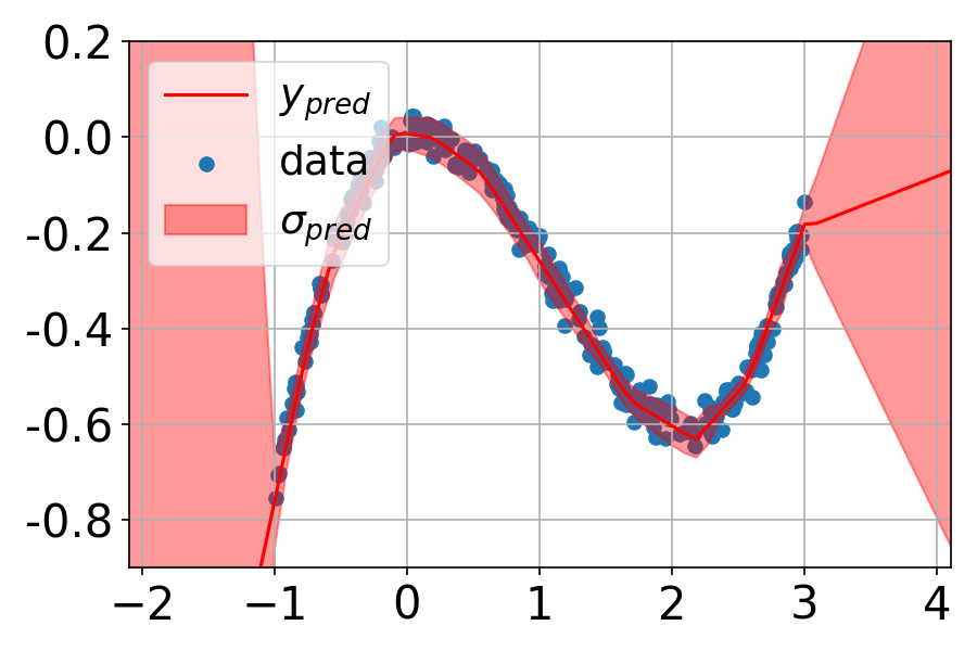
(c)	(d)

Figure 4: Uncertainty Estimation for Regression. The task is to regress $y$-axis values for $x$-axis data points drawn in the range $x\in[-1,3]$ from third power polynomial with added Gaussian noise. Red colored area depicts the uncertainty assigned by different models to individual points on the $x$-axis grid. (a) Single model, (b) MC-Dropout, (c) Deep Ensembles, (d) ZigZag.

Let us now consider the simple regression problem depicted by Fig. 4: We draw values $x$ in the range $[-1,3]$, compute values $y=f(x)+\sigma$ where $f$ is the third order polynomial and $\sigma$ is Gaussian noise, and use these pairs to train a regression network. The shaded areas depict the uncertainty estimated by Single-Model, MC-Dropout, Deep Ensembles, and ZigZag. For the points outside of the training range, the last two correctly predict very large uncertainties, unlike the first two. But again, ZigZag does it at a lower computational cost than Deep Ensembles.

Classification Tasks.

We now compare ZigZag against the baselines on the widely used benchmark datasets MNIST vs FMNIST, CIFAR vs SVHN, and ImageNet vs ImageNet-O. The images are very different across datasets and exhibit distinct statistics. For each dataset pair, we use the first to train the network and to evaluate how well calibrated the methods are the second to perform out-of-domain detection experiments. We report the results in Tab 1. In all three cases, Deep Ensembles and ZigZag perform similarly and outperform the other approaches. However, ZigZag does not incur the 5-fold increase in memory and time requirements that Deep Ensembles does. Even though the other sampling-free approaches tend to yields worse calibration than sampling-based ones (Postels et al. 2021), ZigZag does not.

MNIST vs FashionMNIST.

We train the networks on MNIST (LeCun et al. 1998) and compute the accuracy and calibration metrics. We then use the uncertainty measure they produce to classify images from the test sets of MNIST and FashionMNIST (Xiao, Rasul, and Vollgraf 2017) as being within the MNIST distribution or not to compute the OOD metrics introduced above. We use a standard architecture with four convolution and pooling layers, followed by fully connected layers with ReLU activations.

CIFAR vs SVHN.

	MC-D	DeepE	BatchE	MaskE	Single	SNGP	OC	VarProp	ZigZag
MAE ($\downarrow$)	4.655	4.472	4.699	4.786	4.724	4.819	4.724	4.682	4.630	UTKFACE
rAULC ($\uparrow$)	0.034	0.047	0.043	0.033	0.026	0.031	0.025	0.029	0.045
Size	1x	5x	1x	1x	1x	1x	1x	1x	1x
Inf. Time	5x	5x	5x	5x	1x	1x	1x	1x	2x
Time	1.1x	5x	1.3x	1.2x	1x	1.7x	1.1x	1x	1x
ROC-AUC ($\uparrow$)	0.688	0.755	0.732	0.653	0.564	0.694	0.658	0.662	0.773
PR-AUC ($\uparrow$)	0.884	0.939	0.846	0.830	0.762	0.890	0.843	0.851	0.959
MAE ($\downarrow$)	3.376	3.03	3.03	3.26	3.18	3.16	3.20	3.25	3.10	AIRFOILS
rAULC ($\uparrow$)	0.065	0.062	0.062	0.034	0.008	0.013	0.01	0.015	0.068
Size	1x	5x	1x	1x	1x	1.05x	1x	1x	1x
Inf. Time	5x	5x	5x	5x	1x	1.3x	1.1x	1.4x	2x
Time	1.2x	5x	1.3x	1.3x	1x	1.7x	1.1x	1.1x	1.2x
ROC-AUC ($\uparrow$)	0.897	0.972	0.971	0.923	0.690	0.894	0.874	0.78	0.992
PR-AUC ($\uparrow$)	0.744	0.955	0.942	0.793	0.681	0.767	0.748	0.76	0.987
MAE ($\downarrow$)	0.129	0.101	0.115	0.115	0.121	0.115	0.120	0.119	0.112	CARS
rAULC ($\uparrow$)	0.06	0.10	0.08	0.07	0.03	0.06	0.04	0.03	0.07
Size	1x	5x	1.05x	1.05x	1x	1x	1x	1x	1x
Inf. Time	5x	5x	5x	5x	1x	1.3x	1.1x	1.2x	2x
Time	1.1x	5x	1.2x	1.3x	1x	1.2x	1x	1.1x	1.2x
ROC-AUC ($\uparrow$)	0.851	0.954	0.921	0.926	0.755	0.872	0.831	0.816	0.956
PR-AUC ($\uparrow$)	0.734	0.941	0.867	0.832	0.534	0.751	0.723	0.567	0.974
Simple	✓	✓	✗	✗	-	✓	✗	✗	✓

Table 2: Regression results on Age Prediction (top), Airfoils (middle) and Cars (bottom). As in Table 1 the best two results in each category are shown in bold and correspond to ZigZag and DeepE, except in terms of computation time and memory requirements where ZigZag does much better.

We ran a similar experiment with the CIFAR10 (Krizhevsky, Nair, and Hinton 2014) and SVHN (Netzer et al. 2011) datasets. This is challenging for OOD detection because many of the CIFAR $32\times 32$ images are noisy and therefore hardly distinguishable from each other, which makes the class labels unreliable. As the training set is relatively small, very large models tend to overfit the training data. We therefore use the Deep Layer Aggregation (DLA) (Yu et al. 2018) network for our experiments that tends to outperform standard architectures such as ResNet (He et al. 2016) or VGG (Simonyan and Zisserman 2015) and trained it as recommended in the original paper. We sample our out-of-distribution data from the SVHN dataset that comprises images belonging to classes that are not in CIFAR10, such as road sign digits.

ImageNet vs ImageNet-O

We experimented with the ImageNet dataset (Russakovsky et al. 2015) and its counterpart, ImageNet-O (Hendrycks et al. 2021). The latter is an extension of the original ImageNet dataset, which is designed to evaluate the robustness and generalization capabilities of machine learning models by providing a challenging set of images that are difficult to classify correctly. As in the CIFAR vs. SVHN scenario, this sets up a challenge for Out-of-Distribution (OOD) detection. We use a standard ResNet50 architecture and the training setup from (He et al. 2016).

Influence of the Number of Samples.

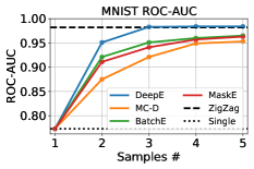
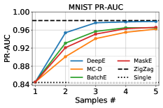
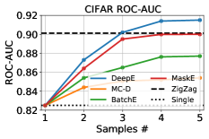
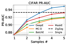
Figure 5: OOD classification performance as a function of the number of samples. The dashed line represents the performance of ZigZag, which is sampling-free.

The five-fold increase in computation time that the sampling-based methods incur is a direct consequence of ours using 5 samples. ZigZag performs two inferences, which is equivalent to using 2 samples. Thus, in Fig 5, we plot OOD classification performance as a function of the number of samples used. Given only 2 or 3 samples, all sampling-based methods do worse than ZigZag. With 4 or 5, Deep-Ensembles is the only one that matches or beats us. However, it then needs at least double the computational budget and memory.

Regression Tasks.

We report similar results for three very different regression tasks in Tab. 2. As for classification tasks, we use data samples significantly different from training ones for OOD evaluation. Then, after generating uncertainty for ID and OOD samples, we evaluate standard AUC metrics as for classification problems. The overall behavior is similar to what we observed for classification. ZigZag performs on par with Deep Ensembles and better than the others, while being much less computationally demanding than Deep Ensembles.

Age Prediction.

First, we consider image-based age prediction from face images. To this end, we use UTKFace (Zhang et al. 2017), a large-scale dataset containing tens of thousands of face images annotated with associated age information. We use a network with a large ResNet-152 backbone and five linear layers with ReLU activations. This architecture yield good performance in terms of accuracy, outperforming the popular ordinal regression model CORAL (Cao, Mirjalili, and Raschka 2020) and matching other state-of-the-art approaches such as (Berg, Oskarsson, and O’Connor 2021). As in the classification experiments described above, we use iCartoonFace (Zheng et al. 2020) dataset as out-of-distribution data. It comprises about $400$k images of cartoon and anime character faces whose pixel statistics are different from those of the UTKFace while exhibiting a semantic similarity. As before, we train our model on the UTKFace training set and use uncertainty to distinguish UTKFace test set images from iCartoonFace ones.

Predicting Lift-to-Drag Ratios.

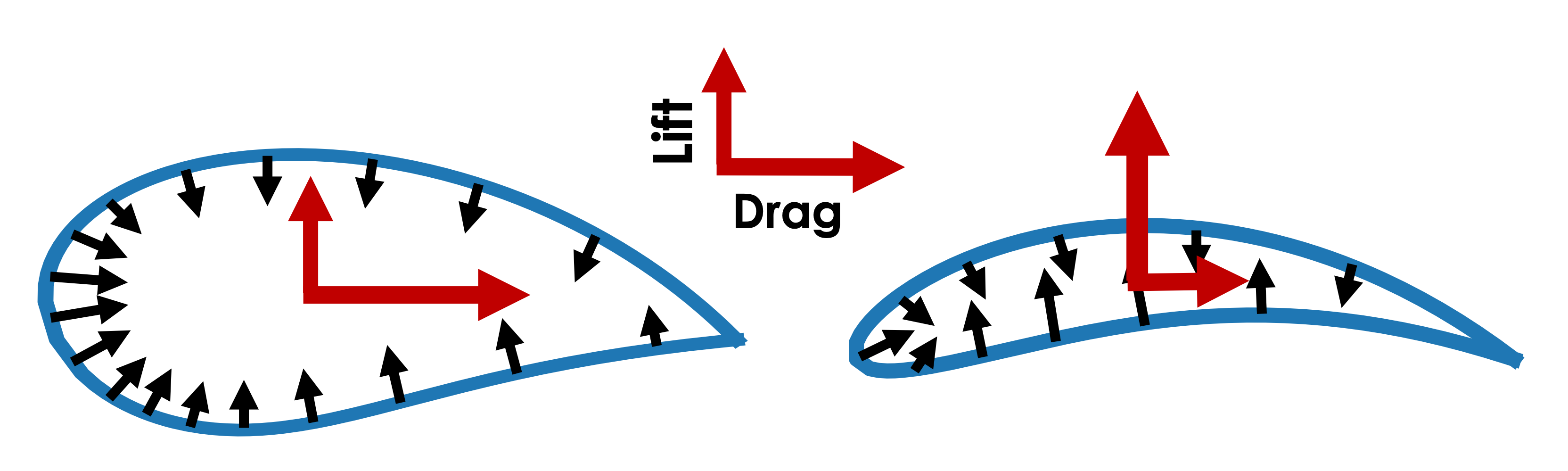
Figure 6: Airfoil Samples. Training and testing profiles (left) have reasonable level of aerodynamics, whereas out-of-distribution samples (right) include only top-notch, but rare, shapes in terms of lift-to-drag ratio. The black arrows represent pressures while the red lines depict overall lift and drag.

Our method is generic and can operate with any kind of data. To demonstrate this, we collected a dataset of $2k$ wing profiles such as those of Fig. 6 by sampling the widely used NACA parameters (Jacobs and Sherman 1937). We then ran the popular XFoil simulator (Drela 1989) to compute the pressure distribution along each profile and estimate its lift-to-drag coefficient, a key measure of aerodynamics performance. The resulting dataset consists of wing profiles $\mathbf{x}_{i}$ represented by a set of 2D nodes and the corresponding scalar lift-to-drag coefficient $\mathbf{y}_{i}$ for $1\leq i\leq 2000$.

We took the $5\%$ of top-performing shapes in terms of lift-to-drag ratio to be the out-of-distribution samples. We took $80\%$ of the remaining $95\%$ as our training set and the rest as our test set. Hence, training and testing shapes span lift-to-drag values from $0$ to $60$, whereas everything beyond that is considered to be OOD and therefore not used for training purposes. We then trained a Graph Neural Network (GNN) that consists of 25 GMM (Monti et al. 2017) layers with ELU nonlinearities (Clevert, Unterthiner, and Hochreiter 2015) and skip connections (He et al. 2016) to predict lift-to-drag $\mathbf{y}_{i}$ from profile $\mathbf{y}_{i}$ for all $i$ in the training set, as in (Remelli et al. 2020; Durasov et al. 2021b). See additional details in the supplementary material.

Predicting the Drag Coefficient of a Car.

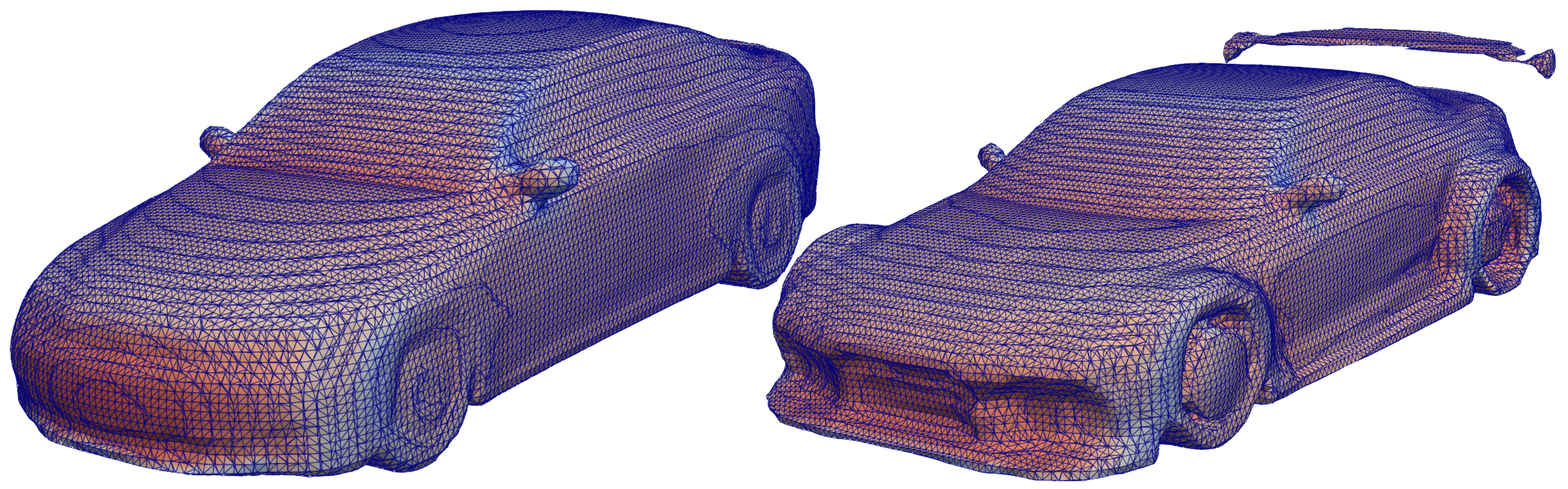
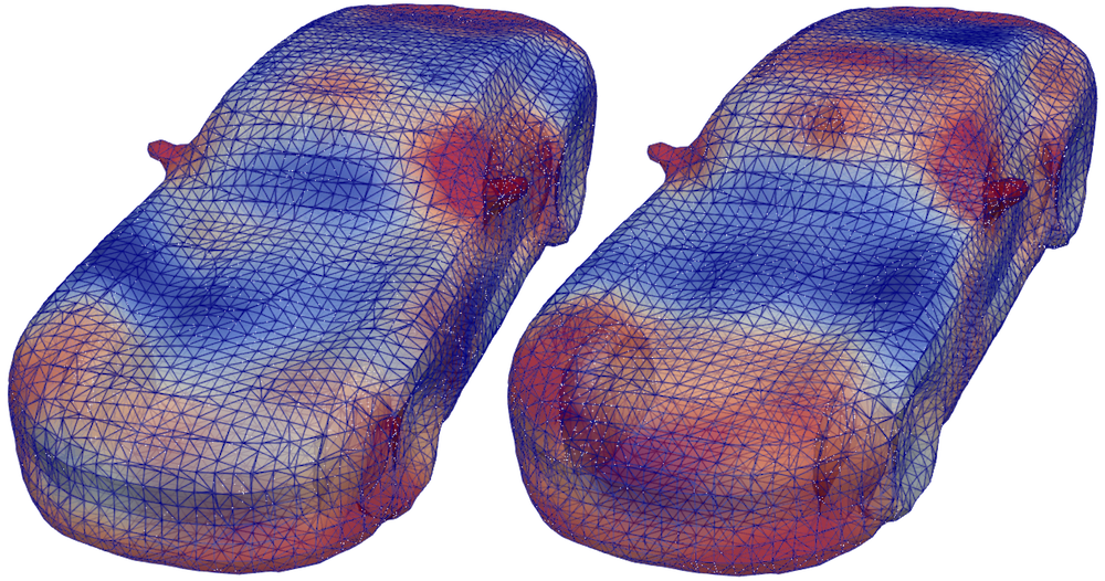
Figure 7: Top: Pressure values. The car dataset comprises many regular vehicles (left) and a few streamlined ones (right), which we treat as being out-of-distribution. Red and blue denote high and low pressures respectively. Bottom: Pressure differences. Large differences in predicted pressure are shown in red and low ones in blue. Ensembles (left) and ZigZag (right) yield the same pattern, with large values mostly in high-curvature areas.

We performed a similar experiment on 3D car models from a subset of the ShapeNet dataset (Chang et al. 2015) that features car meshes that are suitable for CFD simulation. We used the same experimental protocol as for the wings except for relying on OpenFOAM (Jasak et al. 2007) to estimate the drag coefficients and a more sophisticated network to predict it from the triangulated 3D meshes representing the cars, which we also describe in the supplementary material.

	Single	MC-D	DeepE	ZigZag
MAE ($\downarrow$)	22.9	20.3	17.9	19.2
rAULC ($\uparrow$)	0.55	0.62	0.68	0.69
ROC-AUC ($\uparrow$)	0.64	0.74	0.83	0.84
PR-AUC ($\uparrow$)	0.63	0.77	0.84	0.82

Table 3: Pressure Prediction. Accuracy and calibration are computed for individual predictions for each node of the mesh. AUC metrics are computed using averaged uncertainty of the mesh and the same data splits as for the drag prediction task.

To experiment with a higher-dimensional task, we used the same data to train a network to predict not only the drag but also a pressure value at each vertex of a car, as shown at the top of Fig. 7. We used the same train-test split as before along with a modified version of the network we used for drag prediction in which we replaced some convolutional layers by transformer layers (Shi et al. 2020), as explained in the supplementary material. As shown at the bottom of Fig. 7, ZigZag yields per-node uncertainties very similar to those of Deep Ensembles. The most uncertain regions are high curvature parts where pressure changes rapidly. This is reflected by the quantitive results of Tab. 3 that, once again, show ZigZag and Deep Ensembles performing similarly.

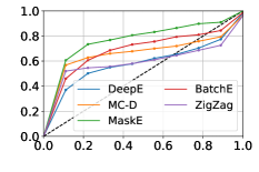
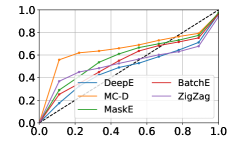
Figure 8: Actual error vs uncertainty estimate for Airfoils (left) and Cars (right) test sets. The $y=x$ curve denotes perfect calibration. ZigZag behaves like ensembles and better than the others.

The rAULC metric we have been reporting aggregates information on how well calibrated the uncertainty estimates are. To better visualize the calibration characteristics of the various methods, we provide actual calibration curves for the airfoil and car aerodynamics regression tasks. In Fig. 8, we plot the cumulative probability of our estimation error being between zero and its maximum value against the cumulative probability of our uncertainty estimate similarly being between its minimum and maximum values, as in (Kendall and Gal 2017). An ideal result would follow the diagonal. ZigZag and DeepE produce the results closest to that, which is consistent with the rAULC calibration results of Tab. 3.

Conclusion

We have proposed an approach to estimating uncertainty that only requires performing a minor change in the first layer of network to accept an additional argument that may be either blank or the result of that prediction. Training the network to yield the same result in both cases enables us to estimate the uncertainty in a principled way and at low computational cost. This approach is applicable to any practical architecture and requires minimal modifications. It is easy to deploy, generic, and delivers results on par with ensembles at a much reduced training budget.

Supplementary Material

In this appendix, we describe the calibration metrics we use and provide additional details about the baselines, training setups, and hyper-parameters used in the experimental section.

Calibration Metrics

In this section, we will describe metrics used for calibration evaluation both for classification and regression tasks. Typical calibration metrics such as Expected Calibration Error (ECE) (Guo et al. 2017) require uncertainties to be express in probabilistic form, which is not the case for many single-shot uncertainty methods. Therefore, unified calibration should be utilized that suits all of the available methods. One of such metrics is Relative Area Under the Lift Curve (rAULC) (Postels et al. 2021) which is based on the Area Under the Lift Curve (Vuk and Curk 2006).

This metric is obtained by ordering the samples according to increasing uncertainty and calculating the accuracy of all samples with an uncertainty value smaller than a particular quantile. More formally, producing uncertainty value $\mathbf{u}_{i}$ for every sample in our evaluation set, we also generate an array of uncertainty quantiles $\textbf{q}_{j}\in[0,1],i\in[1,...,S]$, with the quantile step equal to $1/S$. Iterating over quantiles $\textbf{q}_{j}$, we compute the performance of our model $F(\textbf{q}_{j})$ using only samples for which uncertainty is less than this quantile. Finally, following notation from (Postels et al. 2021) we compute the AULC metric as

$$AULC=-1+\sum^{j=1}_{S}\frac{1}{S}\frac{F(\textbf{q}_{j})}{F_{R}(\textbf{q}_{j})},$$

where $F_{R}(\textbf{q}_{j})$ represents performance for baseline uncertainty that corresponds to random ordering. Further, in order to compute rAULC we divide AULC with the value of AULC produced by ideal (optimal) uncertainty model that perfectly orders all of the samples in order of increasing error. Following (Postels et al. 2021), we use accuracy as $F(\textbf{q}_{j})$ for classification. Similarly, we extend AULC and rAULC to regression tasks via using as $F(\textbf{q}_{j})$ an inverse of Mean Absolute Error (MAE) computed for samples with uncertainties less then $\textbf{q}_{j}$.

Training Details and Baselines

Synthetic Regression

For our synthetic regression experiments, we use the architecture that consists of 6 linear blocks, ELU (Clevert, Unterthiner, and Hochreiter 2015) activations, BatchNorms (Ioffe and Szegedy 2015) and skip-connections (He et al. 2016). We train the model for 4000 epochs using Adam (Kingma and Ba 2015) optimizer with $10^{-2}$ learning rate and mean squared error loss. For Single baseline, we utilize loss from (Kendall and Gal 2017) to enable uncertainty estimation. Deep Ensembles baseline uses 5 trained single models to extract mean and variance from predictions. For MC-Dropout, we apply dropout with 0.2 dropout rate to the last 2 linear layers and sample 5 different predictions during inference. Lastly, for ZigZag we extend the first layer of single model to take two inputs and train it the same way as original model.

Synthetic Classification

For synthetic classification experiments, we adopt simple feed-forward neural network that comprise of 10 linear layers with ELU activation and skip-connections. As for regression, we apply Adam optimizer for 300 epochs and $10^{-2}$ learning rate. Deep Ensembles also consists of 5 models, MC-Dropout drops activations from the last two layers with $0.15$ drop rate, ZigZag extends the first layer of the original model so it is able to process additional inputs.

MNIST

Model used for MNIST experiments consists of two convolutional layers with max polling followed by three linear layers with LeakyReLU activations. We also train this model using Adam optimizer for three epochs with $10^{-2}$ learning rate. MC-Dropout, BatchEnsemble and Masksembles are applied to the last two layers of the model with $0.2$ drop rate for MC-Dropout and $1.5$ scale factor for Masksembles. VarProp propagates variance through the last three linear layers as it was described in (Postels et al. 2019). SNGP applies Random Features (Rahimi and Recht 2007) to the last layer of the model and Spectral Normalization (Miyato et al. 2018) to the rest. OC extracts features after convolutional layers and train five small models that represent certificates.

CIFAR

For CIFAR experiments, we use DLA (Yu et al. 2018) network and adopt original training setup: network is trained with SGD optimizer with $0.9$ momentum for 20 epochs with $10^{-1}$ learning rate and 10 more epochs with $10^{-2}$. As before, MC-Dropout, BatchEnsemble and Masksembles are applied to the last three layers of the model with $0.1$ drop rate and $1.5$ scale factor. Features for OC are taken after convolutional part of the model.

ImageNet

For ImageNet experiments, we use common ResNet50 (He et al. 2016) architecture and follow original training procedure. MC-Dropout, BatchEnsemble and Masksembles are applied to the last five layers of the model with $0.1$ drop rate, $2.0$ scale factor, and each uses 5 samples during inference. Varprop propagates variance through the last five layers of the network. OC uses features from the penultimate layer and trains five small feed-forward networks for certificates.

Age Prediction

As an age predictor, we use common Resnet (He et al. 2016) backbone followed by five linear layers with LeakyReLU activations. As before, MC-Dropout, BatchEnsemble and Masksembles are applied to the last four layers of the model with $0.1$ drop rate and $1.5$ scale factor. Varprop propagates variance through the last five layers of the network. OC uses features from penultimate layer and trains five small feed-forward networks for certificates.

Airfoils Lift-to-Drag

Lift-to-Drag ratio is predicted with custom model that consists of twenty five GMM (Monti et al. 2017) layers, global max pooling and five linear layers with applied ReLU activations. The model is trained for 10 epochs with Adam optimizer and $10^{-3}$ learning rate. All of the uncertainty baselines follow the same setup described for age prediction experiments.

Estimating Car Drag

To predict drag associated to a triangulated 3D car, we utilize similar model to airfoil experiments but with increased capacity. Instead of twenty five GMM layers, we use thirty five and also apply skip-connections with ELU activations. Final model is being trained for 100 epochs with Adam optimizer and $10^{-3}$ learning rate. All of the uncertainty methods are applied to non-graphical part of the model – last five linear layers. As before, MC-Dropout uses $0.05$ drop rate, Masksembles use $1.5$ scale factor, $SNGP$ applies Spectral Normalization to the last five layers and $OC$ extract features right after max pooling layer.

For pressure prediction task, we modified original architecture and replaced GMM layers with Transformer layers (Shi et al. 2020) for more fine-grained predictions. In addition, we use GraphNorm (Cai et al. 2021) after each convolution for faster training and increase total size of the model to seventy layers. The model is being trained for $1500$ epochs with Adam optimizer with $10^{-3}$ learning rate. Implemented uncertainty baselines are replicated from drag prediction experiments.

References

- Amersfoort et al. (2020) Amersfoort, V.; Smith, J. A.; Teh, L. A.; Whye, Y.; and Gal, Y. 2020. Uncertainty Estimation Using a Single Deep Deterministic Neural Network. In International Conference on Machine Learning, 9690–9700.
- Ashukha et al. (2020) Ashukha, A.; Lyzhov, A.; Molchanov, D.; and Vetrov, D. 2020. Pitfalls of In-Domain Uncertainty Estimation and Ensembling in Deep Learning. In International Conference on Learning Representations.
- Berg, Oskarsson, and O’Connor (2021) Berg, A.; Oskarsson, M.; and O’Connor, M. 2021. Deep Ordinal Regression with Label Diversity. In International Conference on Pattern Recognition, 2740–2747.
- Blundell et al. (2015) Blundell, C.; Cornebise, J.; Kavukcuoglu, K.; and Wierstra, D. 2015. Weight Uncertainty in Neural Network. In International Conference on Machine Learning, 1613–1622.
- Brier et al. (1950) Brier, G. W.; et al. 1950. Verification of Forecasts Expressed in Terms of Probability. Monthly weather review, 78(1): 1–3.
- Cai et al. (2021) Cai, T.; Luo, S.; Xu, K.; He, D.; Liu, T.-y.; and Wang, L. 2021. Graphnorm: A principled approach to accelerating graph neural network training. In International Conference on Machine Learning.
- Cao, Mirjalili, and Raschka (2020) Cao, W.; Mirjalili, V.; and Raschka, S. 2020. Rank Consistent Ordinal Regression for Neural Networks with Application to Age Estimation. Pattern Recognition, 140: 325–331.
- Chang et al. (2015) Chang, A.; Funkhouser, T.; G., L.; Hanrahan, P.; Huang, Q.; Li, Z.; Savarese, S.; Savva, M.; Song, S.; Su, H.; Xiao, J.; Yi, L.; and Yu, F. 2015. Shapenet: An Information-Rich 3D Model Repository. In arXiv Preprint.
- Clevert, Unterthiner, and Hochreiter (2015) Clevert, D.-A.; Unterthiner, T.; and Hochreiter, S. 2015. Fast and Accurate Deep Network Learning by Exponential Linear Units (ELUs). In arXiv Preprint.
- Der Kiureghian and Ditlevsen (2009) Der Kiureghian, A.; and Ditlevsen, O. 2009. Aleatory or epistemic? Does it matter? Structural safety, 31(2): 105–112.
- Dosovitskiy et al. (2020) Dosovitskiy, A.; Beyer, L.; Kolesnikov, A.; Weissenborn, D.; Zhai, X.; Unterthiner, T.; Dehghani, M.; Minderer, M.; Heigold, G.; Gelly, S.; Uszkoreit, J.; and Houlsby, N. 2020. An Image is Worth 16x16 Words: Transformers for Image Recognition at Scale. In arXiv Preprint.
- Drela (1989) Drela, M. 1989. XFOIL: An Analysis and Design System for Low Reynolds Number Airfoils. In Conference on Low Reynolds Number Aerodynamics, 1–12.
- Durasov et al. (2021a) Durasov, N.; Bagautdinov, T.; Baque, P.; and Fua, P. 2021a. Masksembles for Uncertainty Estimation. In Conference on Computer Vision and Pattern Recognition.
- Durasov et al. (2021b) Durasov, N.; Lukoyanov, A.; Donier, J.; and Fua, P. 2021b. DEBOSH: Deep Bayesian Shape Optimization. In arXiv Preprint.
- Furno and Vistocco (2018) Furno, M.; and Vistocco, D. 2018. Quantile regression: estimation and simulation, Volume 2, volume 216. John Wiley & Sons.
- Gal (2016) Gal, Y. 2016. Uncertainty in Deep Learning. Ph.D. thesis, University of Cambridge.
- Gal and Ghahramani (2016) Gal, Y.; and Ghahramani, Z. 2016. Dropout as a Bayesian Approximation: Representing Model Uncertainty in Deep Learning. In International Conference on Machine Learning, 1050–1059.
- Gast and Roth (2018) Gast, J.; and Roth, S. 2018. Lightweight Probabilistic Deep Networks. In Conference on Computer Vision and Pattern Recognition.
- Graves (2011) Graves, A. 2011. Practical variational inference for neural networks. Advances in Neural Information Processing Systems, 24.
- Guo et al. (2017) Guo, C.; Pleiss, G.; Sun, Y.; and Weinberger, K. Q. 2017. On Calibration of Modern Neural Networks. In International Conference on Learning Representations.
- He et al. (2016) He, K.; Zhang, X.; Ren, S.; and Sun, J. 2016. Deep Residual Learning for Image Recognition. In Conference on Computer Vision and Pattern Recognition, 770–778.
- Hendrycks et al. (2021) Hendrycks, D.; Zhao, K.; Basart, S.; Steinhardt, J.; and Song, D. 2021. Natural adversarial examples. In Conference on Computer Vision and Pattern Recognition, 15262–15271.
- Hernández-Lobato and Adams (2015) Hernández-Lobato, J. M.; and Adams, R. 2015. Probabilistic Backpropagation for Scalable Learning of Bayesian Neural Networks. In International Conference on Machine Learning, 1861–1869.
- Ioffe and Szegedy (2015) Ioffe, S.; and Szegedy, C. 2015. Batch Normalization: Accelerating Deep Network Training by Reducing Internal Covariate Shift. In International Conference on Machine Learning.
- Jacobs and Sherman (1937) Jacobs, E.; and Sherman, A. 1937. Airfoil Section Characteristics as Affected by Variations of the Reynolds Number. Report-National Advisory Committee for Aeronautics, 227: 577–611.
- Jasak et al. (2007) Jasak, H.; Jemcov, A.; Tukovic, Z.; et al. 2007. OpenFOAM: A C++ Library for Complex Physics Simulations. In International workshop on coupled methods in numerical dynamics.
- Kendall and Gal (2017) Kendall, A.; and Gal, Y. 2017. What Uncertainties Do We Need in Bayesian Deep Learning for Computer Vision? In Advances in Neural Information Processing Systems.
- Kingma and Ba (2015) Kingma, D. P.; and Ba, J. 2015. Adam: A Method for Stochastic Optimisation. In International Conference on Learning Representations.
- Kingma, Salimans, and Welling (2015) Kingma, D. P.; Salimans, T.; and Welling, M. 2015. Variational Dropout and the Local Parameterization Trick. Advances in Neural Information Processing Systems, 28.
- Krizhevsky, Nair, and Hinton (2014) Krizhevsky, A.; Nair, V.; and Hinton, G. 2014. The CIFAR-10 Dataset. online: http://www. cs. toronto. edu/kriz/cifar. html, 55(5).
- Lakshminarayanan, Pritzel, and Blundell (2017) Lakshminarayanan, B.; Pritzel, A.; and Blundell, C. 2017. Simple and Scalable Predictive Uncertainty Estimation Using Deep Ensembles. In Advances in Neural Information Processing Systems.
- LeCun et al. (1998) LeCun, Y.; Bottou, L.; Bengio, Y.; and Haffner, P. 1998. Gradient-Based Learning Applied to Document Recognition. Proceedings of the IEEE, 2278–2324.
- Liu et al. (2020) Liu, J.; Lin, Z.; Padhy, S.; Tran, D.; Weiss, T. B.; and Lakshminarayanan, B. 2020. Simple and Principled Uncertainty Estimation with Deterministic Deep Learning via Distance Awareness. In Advances in Neural Information Processing Systems.
- Loquercio, Segu, and Scaramuzza (2020) Loquercio, A.; Segu, M.; and Scaramuzza, D. 2020. A General Framework for Uncertainty Estimation in Deep Learning. IEEE Robotics and Automation Letters, 5(2): 3153–3160.
- Mackay (1995) Mackay, D. J. 1995. Bayesian Neural Networks and Density Networks. Nuclear Instruments and Methods in Physics Research Section A: Accelerators, Spectrometers, Detectors and Associated Equipment, 354(1): 73–80.
- Malinin et al. (2020) Malinin, A.; Chervontsev, S.; Provilkov, I.; and Gales, M. 2020. Regression Prior Networks. In arXiv Preprint.
- Malinin and Gales (2018) Malinin, A.; and Gales, M. 2018. Predictive Uncertainty Estimation via Prior Networks. In Advances in Neural Information Processing Systems.
- Mi et al. (2022) Mi, L.; Wang, H.; Tian, Y.; He, H.; and Shavit, N. N. 2022. Training-free uncertainty estimation for dense regression: Sensitivity as a surrogate. In AAAI Conference on Artificial Intelligence, 10042–10050.
- Miyato et al. (2018) Miyato, T.; Kataoka, T.; Koyama, M.; and Yoshida, Y. 2018. Spectral Normalization for Generative Adversarial Networks. In International Conference on Learning Representations.
- Monti et al. (2017) Monti, F.; Boscaini, D.; Masci, J.; Rodolà, E.; Svoboda, J.; and Bronstein, M. M. 2017. Geometric Deep Learning on Graphs and Manifolds Using Mixture Model CNNs. In Conference on Computer Vision and Pattern Recognition, 5425–5434.
- Mukhoti et al. (2021a) Mukhoti, J.; Kirsch, A.; van Amersfoort, J.; Torr, P. H.; and Gal, Y. 2021a. Deterministic neural networks with appropriate inductive biases capture epistemic and aleatoric uncertainty. arXiv Preprint.
- Mukhoti et al. (2021b) Mukhoti, J.; van Amersfoort; Torr, J. A.; HS, P.; and Gal, Y. 2021b. Deep Deterministic Uncertainty for Semantic Segmentation. In arXiv Preprint.
- Netzer et al. (2011) Netzer, Y.; Wang, T.; Coates, A.; Bissacco, A.; Wu, B.; and Ng, A. 2011. Reading Digits in Natural Images with Unsupervised Feature Learning. In Advances in Neural Information Processing Systems.
- Nguyen, Yosinski, and Clune (2015) Nguyen, A.; Yosinski, J.; and Clune, J. 2015. Deep Neural Networks are Easily Fooled: High Confidence Predictions for Unrecognizable Images. In Conference on Computer Vision and Pattern Recognition, 427–436.
- Postels et al. (2019) Postels, J.; Ferroni, F.; Coskun, H.; Navab, N.; and Tombari, F. 2019. Sampling-Free Epistemic Uncertainty Estimation Using Approximated Variance Propagation. In Conference on Computer Vision and Pattern Recognition, 2931–2940.
- Postels et al. (2021) Postels, J.; Segu, M.; Sun, T.; Gool, L. V.; Yu, F.; and Tombari, F. 2021. On the Practicality of Deterministic Epistemic Uncertainty. In arXiv Preprint.
- Rahimi and Recht (2007) Rahimi, A.; and Recht, B. 2007. Random Features for Large-Scale Kernel Machines. In Advances in Neural Information Processing Systems, 1177–1184.
- Remelli et al. (2020) Remelli, E.; Lukoianov, A.; Richter, S.; Guillard, B.; Bagautdinov, T.; Baque, P.; and Fua, P. 2020. Meshsdf: Differentiable Iso-Surface Extraction. In Advances in Neural Information Processing Systems.
- Russakovsky et al. (2015) Russakovsky, O.; Deng, J.; Su, H.; Krause, J.; S.Satheesh; Ma, S.; Huang, Z.; Karpathy, A.; Khosla, A.; Bernstein, M.; Berg, A.; and Fei-Fei, L. 2015. Imagenet Large Scale Visual Recognition Challenge. International Journal of Computer Vision, 115(3): 211–252.
- Shekhovtsov and Flach (2019) Shekhovtsov, A.; and Flach, B. 2019. Feed-Forward Propagation in Probabilistic Neural Networks with Categorical and Max Layers. In International Conference on Learning Representations.
- Shi et al. (2020) Shi, Y.; Huang, Z.; Feng, S.; Zhong, H.; Wang, W.; and Sun, Y. 2020. Masked Label Prediction: Unified Message Passing Model for Semi-Supervised Classification. In arXiv Preprint.
- Simonyan, Vedaldi, and Zisserman (2014) Simonyan, K.; Vedaldi, A.; and Zisserman, A. 2014. Learning Local Feature Descriptors Using Convex Optimisation. IEEE Transactions on Pattern Analysis and Machine Intelligence.
- Simonyan and Zisserman (2015) Simonyan, K.; and Zisserman, A. 2015. Very Deep Convolutional Networks for Large-Scale Image Recognition. In International Conference on Learning Representations.
- Tagasovska and Lopez-Paz (2018) Tagasovska, N.; and Lopez-Paz, D. 2018. Frequentist Uncertainty Estimates for Deep Learning. In arXiv Preprint.
- Tagasovska and Lopez-Paz (2019) Tagasovska, N.; and Lopez-Paz, D. 2019. Single-Model Uncertainties for Deep Learning. In Advances in Neural Information Processing Systems.
- Vuk and Curk (2006) Vuk, M.; and Curk, T. 2006. ROC curve, lift chart and calibration plot. Advances in methodology and Statistics, 3(1): 89–108.
- Wang, Shi, and Yeung (2016) Wang, H.; Shi, X.; and Yeung, D.-Y. 2016. Natural-Parameter Networks: A Class of Probabilistic Neural Networks. Advances in Neural Information Processing Systems, 29.
- Wannenwetsch and Roth (2020) Wannenwetsch, A. S.; and Roth, S. 2020. (Probabilistic Pixel-Adaptive Refinement Networks). In Conference on Computer Vision and Pattern Recognition, 11642–11651.
- Weller and Jebara (2014) Weller, A.; and Jebara, T. 2014. Approximating the Bethe Partition Function. In Uncertainty in Artificial Intelligence.
- Wen, Tran, and Ba (2020) Wen, Y.; Tran, D.; and Ba, J. 2020. Batchensemble: An Alternative Approach to Efficient Ensemble and Lifelong Learning. In International Conference on Learning Representations.
- Xiao, Rasul, and Vollgraf (2017) Xiao, H.; Rasul, K.; and Vollgraf, R. 2017. Fashion-Mnist: A Novel Image Dataset for Benchmarking Machine Learning Algorithms. In arXiv Preprint.
- Yu et al. (2018) Yu, F.; Wang, D.; Shelhamer, E.; and Darrell, T. 2018. Deep Layer Aggregation. In Conference on Computer Vision and Pattern Recognition, 2403–2412.
- Zhang et al. (2021) Zhang, C.; Bengio, S.; Hardt, M.; Recht, B.; and Vinyals, O. 2021. Understanding Deep Learning (still) Requires Rethinking Generalization. Communications of the ACM, 64(3): 107–115.
- Zhang et al. (2019) Zhang, Z.; Romero, A.; Muckley, M. J.; Vincent, P.; Yang, L.; and Drozdzal, M. 2019. Reducing uncertainty in undersampled MRI reconstruction with active acquisition. In Conference on Computer Vision and Pattern Recognition, 2049–2058.
- Zhang et al. (2017) Zhang, Z.; Song, Y.; ; and Qi, H. 2017. Age Progression/regression by Conditional Adversarial Autoencoder. In Conference on Computer Vision and Pattern Recognition.
- Zheng et al. (2020) Zheng, Y.; Zhao, Y.; Ren, M.; Yan, H.; Lu, X.; Liu, J.; and Li, J. 2020. Cartoon Face Recognition: A Benchmark Dataset. In Proceedings of the 28th ACM international conference on multimedia, 2264–2272.