Breakdown of the Meissner effect at the zero exceptional point in non-Hermitian two-band BCS model

Abstract

We investigate a non-Hermitian many-body Hamiltonian describing a system coupled to an external bath. Using non-Hermitian mean-field theory, we show that the Hamiltonian’s eigenvalues exhibit a singularity in the parameter space, leading to the emergence of a phase transition point called the exceptional point. At this point, the Meissner effect breaks down while gap parameters remain finite. Our work provides insights into the role of an exceptional point in the non-Hermitian many-body systems.

1 Introduction

Non-Hermitian physics has been a subject of intense theoretical and experimental research over the past few decades, with one of its key features being the eigenvalue’s parameter point known as the ”exceptional point” (EP) [1]. At the EP, the associated Hamiltonian becomes non-diagonalizable and is accompanied by the breakdown of parity time-reversal symmetry of the system [2]. The EPs have been observed in a variety of physical phenomena, such as stopping of light in classical optics [3], quantum phase transitions [4, 5, 6], and more examples to be found in the review paper [7]. Despite significant research on EPs in non-Hermitian one-body systems, their analysis in non-Hermitian many-body systems is still in its early stages both theoretically and experimentally [8, 9, 10, 11, 12, 13, 14, 15, 5, 16, 17, 18, 19, 6]. In this paper, we aim to investigate the role of EPs in non-Hermitian many-body systems.

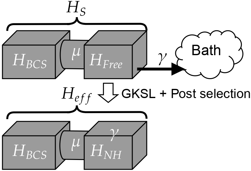
Figure 1: Schemetic of the system Hamiltonian, coupled to the external bath. The large arrow indicates that we have made an appropriate approximation to reduce the system to a non-Hermitian effective Hamiltonian. The bath coupling parameter $\gamma$ becomes one of the parameters in the effective Hamiltonian $H_{\text{eff}}$ after GKSL and post-selection.

A superconductor is characterized by two key macroscopic phenomena: zero electrical resistivity and diamagnetism (Meissner effect). These phenomena are described by the first and second London equations, respectively [20]. Specifically, the equations are $\nabla^{2}\vec{B}\propto n\vec{B}$ and $\partial_{t}\vec{j}\propto n\vec{E}$, where $\vec{B}$, $\vec{j}$, and $\vec{E}$ are the magnetic field, current density, and electric field, respectively. The constant $n$ is proportional to the absolute value of the gap parameter from the Bardeen–Cooper–Schrieffer (BCS) theory [21]. Therefore if the gap parameter is zero, the Meissner effect and zero electrical resistivity phenomena are disrupted, resulting in a breakdown of superconductivity. In this work, we present a novel mechanism for the breakdown of superconductivity, where the constant $n$ becomes zero while the gap parameter remains non-zero. Furthermore, we demonstrate in our example the non-conventional breakdown of superconductivity at the zero exceptional point (0EP) of the macroscopic theory. As such, this phenomenon is unique to non-Hermitian systems. We note that the 0EP [22] is equivalent to the EP, except that it lacks a branch-cut structure often associated with the EP [23].

In this paper, we will utilize our previous study on the breakdown of the Higgs mechanism at the 0EP in the two-component non-Hermitian scalar field theory [24, 25]. Using the correspondence between the Higgs mechanism and the Meissner effect, we will observe that the Meissner effect breaks down at the 0EP while the gap parameters stay finite. Our approach differs from the previous analyses of EP [5, 18] where authors analyzed the EP in the momentum space of the microscopic model. Here we focus on the EP in the parameter space of the macroscopic model.

We aim to find a microscopic theory that admits the two-component complex Ginzburg-Landau model, which was investigated in Refs. [26, 24, 25]. We begin with the BCS, and Free Hamiltonians of different bands, coupled via two-band superconductor-type coupling [27], which is schematically depicted in Fig. 1. The system Hamiltonian is $H_{\text{S}}=H_{\text{BCS}}+H_{\text{Free}}+H_{\text{Int}}$ where individual Hamiltonians are

$$H_{\text{BCS}} = \int d^{3}r\sum_{\sigma=\uparrow,\downarrow}~{}c^{\dagger}_{1\sigma}(\vec{r})\left(-\frac{\nabla^{2}_{r}}{2m_{1}}-\mu_{1}\right)c_{1\sigma}(\vec{r})-gc^{\dagger}_{1\uparrow}(\vec{r})c^{\dagger}_{1\downarrow}(\vec{r})c_{1\downarrow}(\vec{r})c_{1\uparrow}(\vec{r}),$$ (1)

$$H_{\text{Free}} = \int d^{3}r\sum_{\sigma=\uparrow,\downarrow}~{}c^{\dagger}_{2\sigma}(\vec{r})\left(-\frac{\nabla^{2}_{r}}{2m_{2}}-\mu_{2}\right)c_{2\sigma}(\vec{r}),$$ (2)

$$H_{\text{int}} = -\mu\int d^{3}r~{}c_{1\uparrow}^{\dagger}(\vec{r})c_{1\downarrow}^{\dagger}(\vec{r})c_{2\uparrow}(\vec{r})c_{2\downarrow}(\vec{r})+c_{2\uparrow}^{\dagger}(\vec{r})c_{2\downarrow}^{\dagger}(\vec{r})c_{1\uparrow}(\vec{r})c_{1\downarrow}(\vec{r})(\vec{r}).$$ (3)

The creation and the annihilation operators of the two bands are given by $\{c_{1\sigma}^{\dagger},c_{1\sigma}\}$ and $\{c_{2\sigma}^{\dagger},c_{2\sigma}\}$, where $\sigma=\uparrow,\downarrow$. The three coupling constants $g$, $\gamma$, and $\mu$ correspond to the internal coupling of BCS, the coupling between the free theory and the bath, and the coupling between BCS and free theory, respectively, all of which are assumed to be positive. The constants $e$, $\{m_{1},m_{2}\}$ and $\{\mu_{1},\mu_{2}\}$ are the gauge charge, the unnormalized masses of the particle for each band, and the chemical potential for each band, respectively. We note that a similar model was considered in Ref. [28] from the perspective of the fermionic superfluid.

The time evolution of the system’s density matrix is described by the Gorini-Kossakowski-Sudarshan-Lindblad (GKSL) master equation [29, 30], given by $d\rho/dt=-i(H_{\text{NH}}\rho-\rho H_{\text{NH}}^{\dagger})-\frac{i}{\hbar}\left[H_{\text{Lamb}},\rho\right]+i\gamma\int d^{3}rL_{2}(\vec{r})\rho L_{2}^{\dagger}(\vec{r})$, where $H_{\text{NH}}$ is the effective non-Hermitian Hamiltonian defined as $H_{\text{NH}}=H_{\text{free}}-i\gamma/2\int d^{3}rL_{2}^{\dagger}L_{2}$. The Lindblad operators $L_{2}(\vec{r})=c_{2\downarrow}(\vec{r})c_{2\uparrow}(\vec{r})$ and $L^{\dagger}_{2}(\vec{r})=c_{2\uparrow}^{\dagger}(\vec{r})c_{2\downarrow}^{\dagger}(\vec{r})$ create and destroy the two-particle state in the system at a rate of $1/\gamma$. Such two-body loss in BCS superconductor was previously considered in Ref. [14] and recent works have discussed the possibility of two-body losses in the solid-state setup [31, 32]. The Lamb-shift term $H_{\text{Lamb}}$ introduces a real shift in the energy level of the free Hamiltonian $H_{\text{free}}$.

This GKSL master equation approximately capture the dynamics of the system when the coupling between the system and the bath is small and the bath is large enough to maintain the thermal equilibrium (Born-Markov approximation)[33]. Furthermore, the dynamics of the system in a short time scale is approximately dictated by the non-Hermitian Hamiltonian $d\rho/dt=-i(H_{\text{NH}}\rho-\rho H_{\text{NH}}^{\dagger})$, until the quantum jump occur. This is called a post-selection, often used in open quantum systems to obtain the non-Hermitian Hamiltonian [34]. Put simply, our model essentially functions as a standard two-band BCS model with a perturbative effect due to the bath. A simpler setup was previously considered in Ref. [14], but did not consider the Meissner effect. The effective non-Hermitian Hamiltonian, which is depicted schematically in Fig. 1, is given by $H_{\text{eff}}=H_{\text{BCS}}+H_{\text{Int}}+H_{\text{NH}}$.

As a supplementary observation, we mention that the non-Hermitian effective Hamiltonian $H_{\text{NH}}[a^{\dagger}_{2},a_{2}]$ could also be manifested as an effective theory of an ultra-cold atomic gas [5, 8, 35, 28] with recent experimental progress [36]. Furthermore, a small body of work has investigated the Meissner in ultra-cold atom [37, 38]. This correspondence provides a promising avenue for exploring non-Hermitian physics in a controllable laboratory setting.

2 The two-component complex Ginzburg-Landau model

We begin our analysis from the partition function $Z=\int\mathcal{D}\psi_{1}\mathcal{D}\psi_{1}^{\dagger}\mathcal{D}\psi_{2}\mathcal{D}\psi_{2}^{\dagger}\exp(-S)$ where the complex action is given by rewriting the effective Hamiltonian $H_{\text{eff}}$ in terms of coherent-state path integral. The two sets of Grassmannian fields $\{\psi_{1},\psi_{1}^{\dagger}\}$ and $\{\psi_{2},\psi_{2}^{\dagger}\}$ correspond to the coherent states of the creation and the annihilation operators $\{c_{1},c_{1}^{\dagger}\}$ and $\{c_{2},c_{2}^{\dagger}\}$, respectively. The explicit form of the action is given as

$$S = S_{1}[\psi_{1}]+S_{2}[\psi_{2}]+S_{\text{Int}}[\psi_{1},\psi_{2}],$$ (4)

$$S_{1} = \sum_{\sigma=\uparrow\downarrow}\int d^{3}r\psi^{\dagger}_{1}(\vec{r})\left(\partial_{\tau}-\frac{(\nabla_{r}-ie\vec{A})^{2}}{2m_{1}}-\mu_{1}\right)\psi_{1}(\vec{r})-g\psi^{\dagger}_{1\uparrow}(r)\psi^{\dagger}_{1\downarrow}(r)\psi_{1\downarrow}(r)\psi_{1\uparrow}(r),$$ (5)

$$S_{2} = \sum_{\sigma=\uparrow\downarrow}\int d^{3}r\psi^{\dagger}_{2}(\vec{r})\left(\partial_{\tau}-\frac{(\nabla_{r}-ie\vec{A})^{2}}{2m_{2}}-\mu_{2}\right)\psi_{2}(\vec{r})-i\gamma\psi^{\dagger}_{2\uparrow}(r)\psi^{\dagger}_{2\downarrow}(r)\psi_{2\downarrow}(r)\psi_{2\uparrow}(r),~{}~{}~{}~{}$$ (6)

$$S_{\text{Int}} = -\mu\int d^{3}r~{}\psi^{\dagger}_{1\uparrow}(\vec{r})\psi^{\dagger}_{1\downarrow}(\vec{r})\psi_{2\uparrow}(\vec{r})\psi_{2\downarrow}(\vec{r})+\psi^{\dagger}_{2\uparrow}(\vec{r})\psi^{\dagger}_{2\downarrow}(\vec{r})\psi_{1\uparrow}(\vec{r})\psi_{\downarrow}(\vec{r}).$$ (7)

Following the non-Hermitian mean field theory of Ref. [5], we consider the partition function of the auxiliary fields $\{\Delta_{1},\overline{\Delta}_{1}\}$ and $\{\Delta_{2},\overline{\Delta}_{2}\}$: $Z_{\Delta}=\prod_{i=1,2}\int D\overline{\Delta}_{i}D\Delta_{i}\exp\big{[}-\frac{1}{g}\overline{\Delta}_{1}\Delta_{1}-\frac{1}{i\gamma}\overline{\Delta}_{2}\Delta_{2}\frac{\mu}{i\gamma g}(\overline{\Delta}_{1}\Delta_{2}+\overline{\Delta}_{2}\Delta_{1})$, where $\overline{\Delta}_{i}$ is not necessarily a complex conjugate of $\Delta_{i}$ for $i=1,2$. Multiplying the partition function $Z$ by $Z_{\Delta}/Z_{\Delta}$ we find $Z\propto\prod_{i=1,2}\int D\psi_{i}^{\dagger}D\psi_{i}D\overline{\Delta}_{i}D\Delta_{i}\exp(-\tilde{S})$, where $\tilde{S}=S+\frac{1}{g}\overline{\Delta}_{1}\Delta_{1}+\frac{1}{i\gamma}\overline{\Delta}_{2}\Delta_{2}+\frac{\mu}{i\gamma g}(\overline{\Delta}_{1}\Delta_{2}+\overline{\Delta}_{2}\Delta_{1})$. Performing the Hubbard Stranovovich transformation

$$\Delta_{1}\rightarrow\Delta_{1}-g\psi_{1\downarrow}\psi_{1\uparrow}, \overline{\Delta}_{1}\rightarrow\overline{\Delta}_{1}-g\psi^{\dagger}_{1\uparrow}\psi_{1\downarrow}^{\dagger},~{}~{}~{}~{}$$ (8)

$$\Delta_{2}\rightarrow\Delta_{2}-i\gamma\psi_{2\downarrow}\psi_{2\uparrow}, \overline{\Delta}_{2}\rightarrow\overline{\Delta}_{2}-i\gamma\psi^{\dagger}_{2\uparrow}\psi_{2\downarrow}^{\dagger},~{}~{}~{}~{}$$ (9)

and integrating out the Grassmannian fields, we find the effective action only in terms of the auxiliary bosonic fields:

$$S_{\text{eff}} = -\text{Tr}\log\left(\begin{array}[]{cc}i\omega_{n}+\epsilon_{\vec{k}}^{(1)}&\Delta_{1}+\frac{\mu}{i\gamma}\Delta_{2}\\ \overline{\Delta}_{1}+\frac{\mu}{i\gamma}\overline{\Delta}_{2}&i\omega_{n}-\epsilon_{\vec{k}}^{(1)}\end{array}\right)-\text{Tr}\log\left(\begin{array}[]{cc}i\omega_{n}+\epsilon_{\vec{k}}^{(2)}&\Delta_{2}+\frac{\mu}{g_{1}}\Delta_{1}\\ \overline{\Delta}_{2}+\frac{\mu}{g_{1}}\overline{\Delta}_{1}&i\omega_{n}-\epsilon_{\vec{k}}^{(2)}\end{array}\right)$$ (15)

$$+\frac{\mu}{i\gamma g}(\overline{\Delta}_{1}\Delta_{2}+\overline{\Delta}_{2}\Delta_{1})+\frac{1}{g}\overline{\Delta}_{1}\Delta_{1}+\frac{1}{i\gamma}\overline{\Delta}_{2}\Delta_{2},$$

where $\epsilon_{r}^{(i)}\equiv\nabla_{r}^{2}/2m_{i}+\mu_{i}$ for $i=1,2$. Solving the equations of motion $\delta S_{\text{eff}}/\delta\Delta_{i}=0$, and $\delta S_{\text{eff}}/\delta\overline{\Delta}_{i}=0$ for $i=1,2$ and defining the expectation value by the path-integral $\braket{\dots}\equiv\int\mathcal{D}\psi^{\dagger}\mathcal{D}\psi\dots e^{-S}$, one finds the gap equations

$$\begin{array}[]{cc}\frac{1}{g}\left(\Delta_{1}+\frac{\mu}{i\gamma}\Delta_{2}\right)=\braket{\psi_{1\downarrow}\psi_{1\uparrow}}+\frac{\mu}{g}\braket{\psi_{2\downarrow}\psi_{2\uparrow}},&\frac{1}{g}\left(\overline{\Delta}_{1}+\frac{\mu}{i\gamma}\overline{\Delta}_{2}\right)=\braket{\psi_{1\uparrow}^{\dagger}\psi_{1\downarrow}^{\dagger}}+\frac{\mu}{g}\braket{\psi_{2\uparrow}^{\dagger}\psi_{2\downarrow}^{\dagger}}\\ \frac{1}{i\gamma}\left(\Delta_{2}+\frac{\mu}{g}\Delta_{1}\right)=\braket{\psi_{2\downarrow}\psi_{2\uparrow}}+\frac{\mu}{i\gamma}\braket{\psi_{1\downarrow}\psi_{1\uparrow}},&\frac{1}{i\gamma}\left(\overline{\Delta}_{2}+\frac{\mu}{g}\overline{\Delta}_{1}\right)=\braket{\psi_{2\uparrow}^{\dagger}\psi_{2\downarrow}^{\dagger}}+\frac{\mu}{i\gamma}\braket{\psi_{1\uparrow}^{\dagger}\psi_{1\downarrow}^{\dagger}}\end{array}$$ (16)

Let us comment on the auxiliary bosonic fields. If we assume $\overline{\Delta}_{i}$ to be the complex conjugate of $\Delta_{i}$, then the gap equations (16) can not be solved for $\Delta_{i}$. Such incompatibility of equations is a common problem in non-Hermitian systems [24, 22, 25], where there are several ways to resolve this issue. Here, we will adopt the approach outlined in Ref. [5] and leave $\overline{\Delta}_{i}$ to be independent of $\Delta_{i}$.

To investigate the Meissner effect of our model, we expand the trace-log term of the effective action (15) to obtain the macroscopic theory. The expansion is most conveniently performed with respect to the combined fields $\Delta_{\epsilon}\equiv\Delta_{1}+i\epsilon\Delta_{2}$, $\Delta_{\delta}\equiv\Delta_{2}+\delta\Delta_{1}$, $\overline{\Delta}_{\epsilon}\equiv\overline{\Delta}_{1}+i\epsilon\overline{\Delta}_{2}$ and $\overline{\Delta}_{\delta}\equiv\overline{\Delta}_{2}+\delta\overline{\Delta}_{1}$, where $\epsilon=\mu/\gamma$ and $\delta=\mu/g$ are dimensionless parameters. However, it is necessary to solve the gap equations (16) to justify the expansion of the effective action around the critical temperature where the combined fields vanish.

2.1 The gap equation

To obtain numerical solutions for the gap equations (16), we employ the approximations $\epsilon\ll\delta\ll 1$ and truncate the equations up to, but not including, terms of order $\delta\epsilon$. This hierarchy corresponds to $\gamma\gg g\gg\mu$. It is worth noting that this approximation scheme has been chosen for illustrative purposes, and other alternatives remain for future investigation.

We numerically solve the simplified gap equation obtained using the above approximation. Details of the calculation are provided in the appendix A, as this is not the main focus of this paper. The solutions are presented in Fig. 2, where we have taken Al (Aluminium) as a BCS superconductor with a density of states at the Fermi level of $\nu_{1}=\sqrt{11.7},\text{eV}$ and $1/g\nu_{1}=1/0.39$ as reported in Ref. [39]. For the free theory $H_{0}[c_{2},c_{2}^{\dagger}]$, we use the density of states $\nu_{2}=\sqrt{9.47},\text{eV}$ of Zn (Zinc). We emphasize that these experimental values are chosen for illustrative purposes and that the experimental realization of our model is left for future research. We further note that the rest of the derivation of this manuscript does not depends on the experimental values chosen above and our main result discussed in section 3 is independent of the experimental values chosen above.

In Fig. 2, we plot the gap parameters $|\Delta_{1}(T)|/\Delta^{\text{BCS}}_{0}$ and $\sqrt{\overline{\Delta}_{2}\Delta_{2}(T)}/\Delta^{\text{BCS}}_{0}$ as a function of the dimensionless parameter $T/T^{\text{BCS}}_{c}$, where $T^{\text{BCS}}_{c}$ is the critical temperature of the BCS theory and $\Delta^{\text{BCS}}_{0}\equiv\Delta^{\text{BCS}}(T=0)$ is the zero-temperature gap parameter for the BCS theory [21]. We find that $|\Delta_{1}|=\sqrt{\overline{\Delta}_{1}\Delta_{1}}$ is real, while $\sqrt{\overline{\Delta}_{2}\Delta_{2}}$ is complex.

The results presented in Fig. 2 confirm that the gap parameters remain small in the vicinity of the critical temperature, thus justifying the expansion of the trace-log term in the effective action (15).

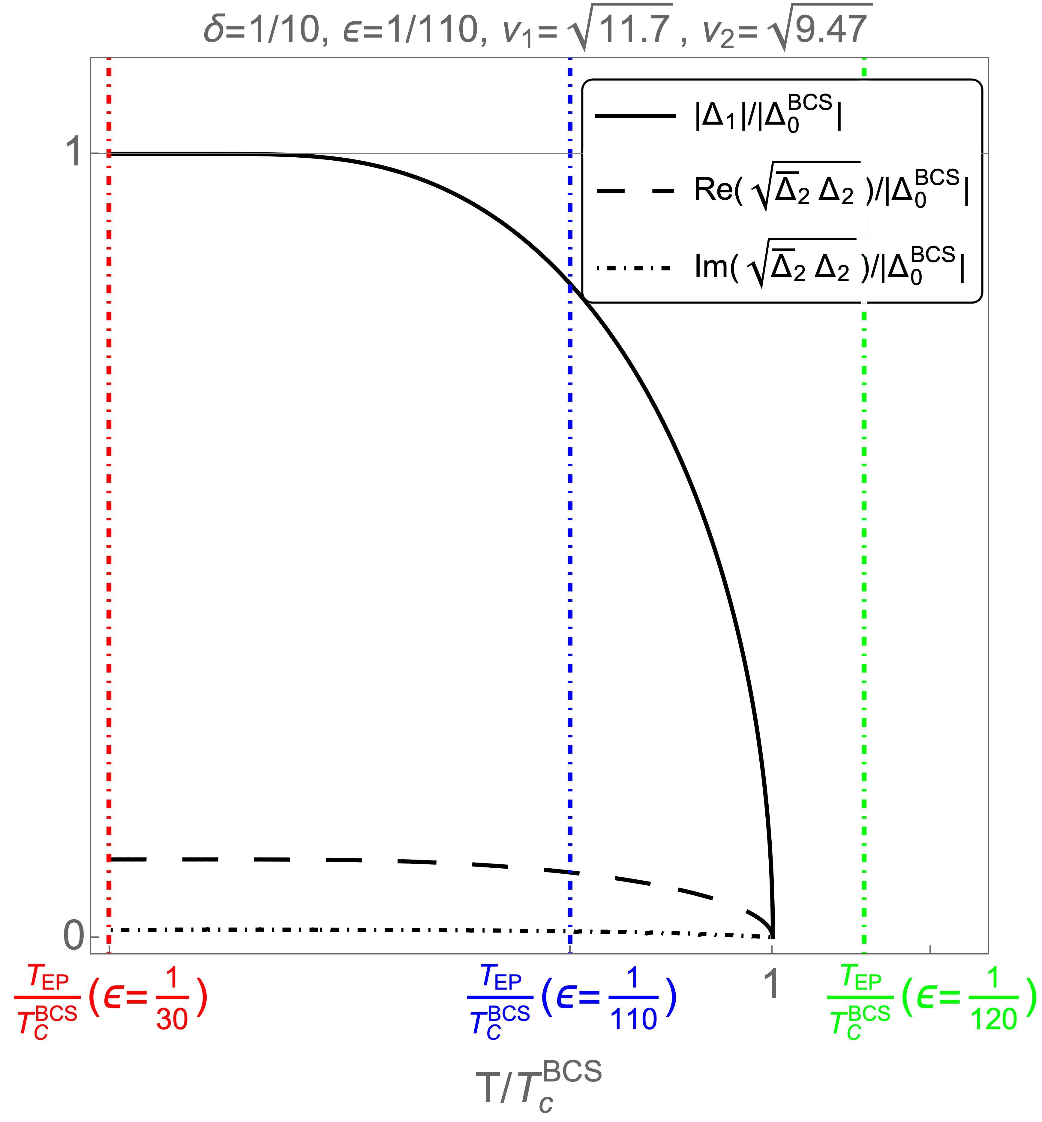
Figure 2: The figure displays numerical solutions for the gap parameters as a function of temperature, obtained from the gap equations $\delta S_{\text{eff}}/\delta\Delta_{1}=0$ and $\delta S_{\text{eff}}/\delta\Delta_{2}=0$ with the approximation $\epsilon\ll\delta\ll 1$, neglecting terms of order $\delta\epsilon$. The parameters used are $1/g\nu_{1}=1/0.39$, $\nu_{1}=\sqrt{11.7}$, $\nu_{2}=\sqrt{9.47}$, and $\delta=1/10$ with $\epsilon=1/110$. The solid and dotted lines represent the real and imaginary parts of the solutions, respectively. The figure also includes three vertical lines corresponding to the exceptional temperatures for $\epsilon=1/30$, $\epsilon=1/110$, and $\epsilon=1/120$, respectively, where the Meissner effect breaks down.

2.2 Two-component complex Ginzburg-Landau model

We expand the effective action (15) with respect to the combined fields $\Delta_{\epsilon}$ and $\Delta_{\delta}$. Note that the gap parameters shown in Fig. 2 is obtained by truncating the gap equations at the order $\delta\epsilon$. However, truncating the effective action up to order $\delta\epsilon$ would not give the appropriate gap equations of order $\delta\epsilon$ because gap parameters $\Delta_{\epsilon}$ and $\Delta_{\delta}$ also scales as $\Delta_{2}=\mathcal{O}(\delta)\Delta_{1}$ from Eq. (53). Therefore, our procedure is to (i) expand the action with respect to $\Delta_{\epsilon}$ and $\Delta_{\delta}$ up to all orders, (ii) calculate the equations of motion with respect to $\overline{\Delta}_{1}$ and $\overline{\Delta}_{2}$, (iii) cut off the equations of motion at the first order $\delta\epsilon$, and (iv) find the corresponding effective action of the equations of motion. We also make the approximation that the dynamical terms are $\nabla_{i}\overline{\Delta}_{\epsilon}\nabla_{i}\Delta\epsilon\sim\nabla_{i}\overline{\Delta}_{1}\nabla_{i}\Delta_{1}$ and $\nabla_{i}\overline{\Delta}_{\delta}\nabla_{i}\Delta_{\delta}\sim\nabla_{i}\overline{\Delta}_{2}\nabla_{i}\Delta_{2}$.

Step (i): We expand the effective action to all orders, which yields

$$\!\!S_{\text{eff}}\!\! = \!\!\int d^{3}r~{}\alpha_{1}\nabla_{i}\overline{\Delta}_{1}\nabla_{i}\Delta_{1}+r_{1}\overline{\Delta}_{\epsilon}\Delta_{\epsilon}+u_{1}(\overline{\Delta}_{\epsilon}\Delta_{\epsilon})^{2}\alpha_{2}\nabla_{i}\overline{\Delta}_{2}\nabla_{i}\Delta_{2}+r_{2}\overline{\Delta}_{\delta}\Delta_{\delta}+u_{2}(\overline{\Delta}_{\delta}\Delta_{\delta})^{2}$$ (17)

$$-\frac{1}{g}\left[\overline{\Delta}_{1}\Delta_{1}-i\frac{\epsilon}{\delta}\overline{\Delta}_{2}\Delta_{2}-i\epsilon\left(\overline{\Delta}_{1}\Delta_{2}+\overline{\Delta}_{2}\Delta_{1}\right)\right],$$

where each coefficients are given by $\alpha_{i}(T)\propto\nu_{i}/T^{2}$, $u_{i}(T)\propto\nu_{i}/T^{3}$ and

$$r_{i}(T) = \frac{T}{V}\sum_{n,\vec{p}}\frac{1}{(\omega_{n}^{2}+(\epsilon^{(i)}_{\vec{p}})^{2})}=\frac{\nu_{i}}{2}\int_{0}^{\frac{\omega_{D}}{2T}}dx\frac{\tanh(x)}{x}\equiv\nu_{i}r(T)\sim\frac{\nu_{i}}{2}\log\left(\frac{2e^{\gamma}\omega_{D}}{\pi T}\right)$$ (18)

as $T\rightarrow 0$. Here we have defined $r(T):=\frac{1}{2}\int_{0}^{\frac{\omega_{D}}{2T}}dx\frac{\tanh(x)}{x}$.

Step (ii): Let us take a functional derivative of the potential of the complex action (17).

$$\frac{\delta S_{\text{eff}}}{\delta\overline{\Delta}_{1}} = r_{1}\Delta_{\epsilon}+2u_{1}\left(\overline{\Delta}_{\epsilon}\Delta_{\epsilon}\right)\Delta_{\epsilon}+\delta r_{2}\Delta_{\delta}+2\delta u_{2}\left(\overline{\Delta}_{\delta}\Delta_{\delta}\right)\Delta_{\delta}-\frac{1}{g}\Delta_{1}+i\frac{1}{g}\epsilon\Delta_{2},$$ (19)

$$\frac{\delta S_{\text{eff}}}{\delta\overline{\Delta}_{2}} = r_{2}\Delta_{\delta}+2u_{2}\left(\overline{\Delta}_{\delta}\Delta_{\delta}\right)\Delta_{\delta}-i\epsilon r_{1}\Delta_{\epsilon}-i\epsilon 2u_{1}\left(\overline{\Delta}_{\epsilon}\Delta_{\epsilon}\right)\Delta_{\epsilon}+i\frac{1}{g}\frac{\epsilon}{\delta}\Delta_{2}+i\frac{1}{g}\epsilon\Delta_{1},$$ (20)

where $\Delta_{\epsilon}=\Delta_{1}-i\epsilon\Delta_{2}$ and $\Delta_{\delta}=\Delta_{2}+\delta\Delta_{1}$.

Step (iii): Using the scaling relation $\Delta_{2}=\mathcal{O}(\delta)\Delta_{1}$ from Eq. (53), we can truncate the equations of motion:

$$0 = (r_{1}-\frac{1}{g}+\delta^{2}r_{2})\Delta_{1}+2u_{1}(\overline{\Delta}_{1}\Delta_{1})\Delta_{1}+r_{2}\delta\Delta_{2},\quad\quad$$ (21)

$$0 = (-i\epsilon r_{1}+\delta\{r_{2}-\frac{1}{g}\frac{\epsilon}{i\delta}\})\Delta_{1}+(r_{2}-\frac{1}{g}\frac{\epsilon}{i\delta})\Delta_{2}.\quad\quad$$ (22)

The consistency check of the above equations with the simplified gap equations obtained from the microscopic approach is presented in the appendix B.

Step (iv): The corresponding complex action of the equations of motion (21) and (22) is

$$S_{\text{eff}} = \int d^{3}r~{}\alpha_{1}\nabla_{i}\overline{\Delta}_{1}\nabla_{i}\Delta_{1}+\left(r_{1}-\frac{1}{g}+r_{2}\delta^{2}\right)\overline{\Delta}_{1}\Delta_{1}+u_{1}\left(\overline{\Delta}_{1}\Delta_{1}\right)^{2}$$

$$+\alpha_{2}\nabla_{i}\overline{\Delta}_{2}\nabla_{i}\Delta_{2}+\left(r_{2}-\frac{1}{g}\frac{\epsilon}{i\delta}\right)\overline{\Delta}_{2}\Delta_{2}+\left(-i\epsilon r_{1}+\delta\left\{r_{2}-\frac{1}{g}\frac{\epsilon}{i\delta}\right\}\right)\left(\overline{\Delta}_{1}\Delta_{2}+\overline{\Delta}_{2}\Delta_{1}\right)$$

Notice that the above action decouples to the standard Ginzburg-Landau model and the free field theory by taking $\mu=0$.

3 The breakdown of the Meissner effect at the (zero) exceptional point

In the previous section, we obtained a two-component complex Ginzburg-Landau model by perturbing with respect to $\epsilon$ and $\delta$. This effective action, given by Eq. (2.2), has also been considered by us and other authors [25, 24] in the context of particle physics, where a breakdown of the Higgs mechanism occurs at a parameter limit known as the 0EP. In this section, we present our main result: the Meissner effect breaks down at the 0EP, while the gap parameters remain finite.

To analyze the Meissner effect, we introduce a classical magnetic field through the minimal coupling $\nabla_{\vec{r}}\rightarrow\nabla_{\vec{r}}+e\vec{A}$, where $\vec{A}$ is the gauge field, and add the kinetic term of the Magnetic field $S_{\text{Mag}}=\int~{}\kappa(\nabla\times\vec{A})^{2}$ to the effective action (15), where the magnetic field is defined by $\vec{B}\equiv\nabla\times\vec{A}$. Taking a functional derivative of the action with respect to the gauge field $\vec{A}$ gives the equations of motion $\delta S_{\text{eff}}/\delta A_{i}=0$. Inserting the constant solutions $\{\Delta_{i},\overline{\Delta}_{i}\}$ for $i\in\{1,2\}$ and acting with $\nabla\times$, we arrive at the extended London equation for the non-Hermitian two-band BCS model: $\nabla^{2}\vec{B}=2e^{2}\alpha_{1}/\kappa\left(\overline{\Delta}_{1}\Delta_{1}+\frac{\alpha_{2}}{\alpha_{1}}\overline{\Delta}_{2}\Delta_{2}\right)\vec{B}$. We say that the Meissner effect is broken when the right-hand side of this equation is zero.

Inserting the solutions of the equations of motion of the effective action (2.2), which are given explicitly in the next section, we have

$$\nabla^{2}\vec{B} = \frac{2e^{2}\alpha_{2}}{\kappa}\overline{\Delta}_{1}\Delta_{1}\vec{B}\left[1+\nu\left(-\delta+\frac{\epsilon}{\gamma}\frac{r_{1}}{r_{2}^{2}+\frac{1}{\gamma^{2}}}+i\epsilon\frac{r_{1}r_{2}}{r_{2}^{2}+\frac{1}{\gamma^{2}}}\right)^{2}\right],$$ (24)

where we denoted $\nu\equiv\nu_{2}/\nu_{1}$ for brevity. The quantity in the square bracket vanishes when the following two equations are simultaneously satisfied:

$$-\delta+\frac{\epsilon}{\gamma}\frac{r_{1}}{r_{2}^{2}+\frac{1}{\gamma^{2}}}=0,~{}~{}1-\nu\epsilon^{2}\left(\frac{r_{1}r_{2}}{r_{2}^{2}+\frac{1}{\gamma^{2}}}\right)^{2}=0.$$ (25)

Two equations can be combined into one, giving $1=\nu\delta^{2}\gamma^{2}r_{2}^{2}$. Writing the explicit form of $r_{2}$ given in Eq. (18), we find $\frac{1}{\nu_{1}}\frac{T}{V}\sum_{n,\vec{p}}1/(\omega_{n}^{2}+(\epsilon^{(1)}_{\vec{p}})^{2})=(1/g\nu_{1})(\epsilon/\delta^{2}\nu\sqrt{\nu})$. We can solve this equation in the standard way and find the temperature $T_{\text{EP}}$ at which the above equations are satisfied:

$$\frac{T_{\text{EP}}}{T_{c}^{\text{BCS}}}=e^{\frac{1}{g\nu_{1}}-\frac{1}{g\nu_{1}}\left(\frac{\epsilon}{\delta^{2}}\frac{1}{\nu\sqrt{\nu}}\right)},$$ (26)

where $T_{c}^{\text{BCS}}$ is the BCS critical temperature. We refer to the above temperature as the exceptional temperature.

The exceptional temperatures $T_{\text{EP}}$ are indicated as vertical lines in Fig. 2 for $1/g\nu_{1}=1/0.39$, $\nu_{1}=\sqrt{11.7}$, $\nu_{2}=\sqrt{9.47}$, and $\delta=1/10$, with three values of the parameters $\epsilon=1/30$, $\epsilon=1/110$, and $\epsilon=1/120$. The gap parameters ${\Delta_{1},\Delta_{2}}$ are only plotted for $\epsilon=1/110$, as the plots for $\epsilon=1/30$ and $\epsilon=1/120$ are indistinguishable from that of $\epsilon=1/110$. Importantly, the gap parameters $\Delta_{1}$ and $\Delta_{2}$ remain finite at $T_{\text{EP}}$, indicating that the Meissner effect breaks down at this exceptional temperature while the gap parameters remain finite.

In the next section, we will show that the exceptional temperature $T_{\text{EP}}$ is equivalent to the EP of the macroscopic theory (2.2). However, before proceeding, we would like to note a few additional features of the exceptional temperature $T_{\text{EP}}$.

The exceptional temperature $T_{\text{EP}}$ starts near zero when $\epsilon=1/30$, approaches the BCS critical temperature $T^{\text{BCS}}_{c}$ when $\epsilon=1/110$, and surpasses $T^{\text{BCS}}_{c}$ when $\epsilon=1/120$, where the breakdown of the Meissner effect is trivial due to the gapless structure for $T>T^{\text{BCS}}_{c}$. This behavior indicates a restricted range of $\epsilon$ where the exceptional temperature $T_{\text{EP}}$ is detectable before it is obscured by $T^{\text{BCS}}_{c}$.

The reason for this mechanism can be seen from the explicit form of the exceptional temperature (26), which is equal to the BCS critical temperature when the exponent $(1-\epsilon/\delta^{2}\nu\sqrt{\nu})/g\nu_{1}$ is zero. Therefore, we identify the detectable region of the exceptional temperature to be $\left(\mu/g\right)^{2}\left(\nu_{1}/\nu_{2}\right)^{3/2}<\mu/\gamma$, and the undetectable regions to be $\left(\mu/g\right)^{2}\left(\nu_{1}/\nu_{2}\right)^{3/2}>\mu/\gamma$. Hence, we conclude that a careful balance of the three parameters $\mu$, $g$, and $\gamma$ is necessary to realize the exceptional temperature within the detectable range $T_{\text{EP}}<T^{\text{BCS}}_{c}$.

In the last section, we will discuss the mathematical origin of the 0EP in our complex Ginzburg-Landau model.

3.1 Connection to the zero exceptional point

Let us analyze the spontaneous symmetry breaking of the effective action (15). The same form of this action was analyzed in the particle-physics context by several authors [25, 24, 26, 40, 13], where it was discovered that at the parameter point dubbed the zero EP [22], the action becomes non-diagonalizable, the gauge masses vanish [25, 24] and the t’Hooft Polyakov monopole masses vanish [41].

To simplify the effective action given by Eq. (2.2), we define $a_{1}\equiv r_{1}-\frac{1}{g}+r_{2}\delta^{2}$, $a_{2}\equiv r_{2}-\frac{1}{i\gamma}$, $b\equiv-i\epsilon r_{1}+\delta r_{2}+i\epsilon/g$. We further simplify the effective action by decomposing the first gap parameter: $\Delta_{1}=\phi_{1}+i\chi_{1}$, $\overline{\Delta}_{1}=\phi_{1}-i\chi_{1}$, where $\phi_{1},\chi_{1}\in\mathbb{R}$. This decomposition is justified by our approximation $\delta\epsilon\ll 1$ where the solution $\overline{\Delta}_{1}\Delta_{1}$ is real (see Fig. 2). The simplified effective action now has a $U(1)$ symmetry on the first gap parameter $\Delta_{1}\rightarrow e^{i\theta}\Delta_{1}$ and $\overline{\Delta}_{1}=\Delta_{1}^{\dagger}\rightarrow e^{-i\theta}\Delta^{\dagger}_{1}$ where $\theta\in\mathbb{R}$.

The equations of motion $\delta S_{\text{eff}}/\delta\phi=0$, where $\phi\in\{\phi_{1},\chi_{1},\Delta_{2},\overline{\Delta}_{2}\}$, admit a vacuume solution $\phi_{1}=0$, $(\chi_{1})^{2}=-\left(a_{1}-b^{2}/a_{2}\right)/2u_{1}$, $\Delta_{2}=-\frac{b}{a_{2}}({\phi_{1}}+i{\chi_{1}})$, and $\overline{\Delta}_{2}=-\frac{b}{a_{2}}({\phi_{1}}-i{\chi_{1}})$.

The Tayler expansion of the effective action around this vacuum solution is

$$S_{\text{eff}} = \int d^{3}r\overline{\Phi}\left(\begin{array}[]{cc}-\alpha_{1}\Box+\frac{b^{2}}{a_{2}}&b\\ b&-\alpha_{2}\Box+a_{2}\end{array}\right)\Phi+\dots$$ (29)

$$= \int d^{3}r\overline{\Phi}D\left[-\Box\mathbb{I}+\left(\begin{array}[]{cc}\frac{1}{\nu_{1}}\frac{b^{2}}{a_{2}}&\frac{1}{\nu_{1}}b\\ \frac{1}{\nu_{2}}b&\frac{1}{\nu_{2}}a_{2}\end{array}\right)\right]\Phi+\dots$$ (32)

$$= \int d^{3}r\overline{\Phi}D\left[-\Box\mathbb{I}+U\left(\begin{array}[]{cc}0&0\\ 0&\lambda\end{array}\right)U^{\dagger}\right]\Phi+\dots$$ (35)

where $\Box=\partial_{\mu}\partial_{\mu}$, $\Phi=(\phi_{1},\Delta)^{T}$, $\overline{\Phi}=(\phi_{1},\overline{\Delta})$, $D=\text{diag}(\nu_{1}/T^{2},\nu_{2}/T^{2})$, and $\nu_{2}\lambda=a_{2}+\nu b^{2}/a_{2}$. The ellipsis contains terms with $\chi_{1}$ and $\Delta_{2}$ and the last line shows that the action has been diagonalized with the unitary matrix $U$. Notice that this expansion breaks and $U(1)$ symmetry and introduces the Goldstone massless field as one can see from Eq. (35).

The $2\times 2$ mass matrix given in Eq. (32) fails to diagonalize when the parameters satisfy $\nu b^{2}/a_{2}^{2}+1=0$, which corresponds to the 0EP of the effective action in Eq. (15). By substituting the specific expressions for $b$ and $a_{2}$, we obtain the condition for non-diagonalizability of the mass matrix in Eq. (32) as a function of the parameters $\{\delta,\epsilon,r_{1},r_{2}\}$:

$$1+\nu\left(-\delta+\frac{\epsilon}{\gamma}\frac{r_{1}}{r_{2}^{2}+\frac{1}{\gamma^{2}}}+i\epsilon\frac{r_{1}r_{2}}{r_{2}^{2}+\frac{1}{\gamma^{2}}}\right)^{2}=0.$$ (36)

The quantity mentioned is precisely the one that appears on the right-hand side of the extended London equation (24). Therefore, the mass matrix in Eq. (32) is non-diagonalizable at the exceptional temperature given by Eq. (26). We can then infer that the Meissner effect breaks down at the zero EP, while the gap parameters remain finite.

4 Conclusion

We began by considering a two-band model weakly coupled to an external bath (see Fig. 1), which can be reduced to a non-Hermitian two-band BCS model through the GKSL master equation. Employing the non-Hermitian mean field theory introduced in Ref. [5] and path integral methods, we derive a corresponding macroscopic model that leads to a two-component Ginzburg-Landau model Eq. (2.2). By analyzing the Meissner effect of this model, we identified a temperature different from the critical temperature at which the Meissner effect breaks down while maintaining a finite gap parameter. We term this temperature the ”exceptional temperature” and find it to be formally equivalent to the 0EP of the complex Ginzburg-Landau model studied in the context of particle physics [25, 24].

In this work, we demonstrate the breakdown of the Meissner effect for a specific example, leaving open the question of whether this is a general feature of non-Hermitian microscopic models. The extended London equation Eq. (24) has acquired a complex part, leading to an oscillatory magnetic field solution, absent in the Hermitian case. Our findings suggest high sensitivity of the exceptional temperature to small variations in the coupling parameter $\epsilon$ compared to the gap parameter, motivating further research. Finally, while our current setup is a toy model, it provides insights into the role of EPs in open systems. However, realizing this setup experimentally is challenging, and more realistic systems remain to be explored in future work.

Appendix A Gap equation

In this section, we derive the gap parameters plotted in Fig. 2, which are solutions to the gap equations $\delta S_{\text{eff}}/\delta\Delta_{1}=0$, $\delta S_{\text{eff}}/\delta\overline{\Delta}_{1}=0$, $\delta S_{\text{eff}}/\delta\Delta_{2}=0$ and $\delta S_{\text{eff}}/\delta\overline{\Delta}_{2}=0$.

Taking the functional derivative of the effective action (15), we find the following coupled gap equations

$$\frac{\delta S_{\text{eff}}}{\delta\overline{\Delta}_{1}} = \frac{1}{g}-\frac{T}{V}\sum_{n,\vec{p}}\frac{1}{\omega_{n}^{2}+(\epsilon^{(1)}_{\vec{p}})^{2}+\overline{\Delta}_{\epsilon}\Delta_{\epsilon}}-\frac{\mu}{g}\frac{\Delta_{\delta}}{\Delta_{\epsilon}}\frac{T}{V}\sum_{n,\vec{p}}\frac{1}{\omega_{n}^{2}+(\epsilon^{(2)}_{\vec{p}})^{2}+\overline{\Delta}_{\delta}\Delta_{\delta}}=0,$$ (37)

$$\frac{\delta S_{\text{eff}}}{\delta\overline{\Delta}_{2}} = \frac{1}{i\gamma}-\frac{T}{V}\sum_{n,\vec{p}}\frac{1}{\omega_{n}^{2}+(\epsilon^{(2)}_{\vec{p}})^{2}+\overline{\Delta}_{\delta}\Delta_{\delta}}-\frac{\mu}{i\gamma}\frac{\Delta_{\epsilon}}{\Delta_{\delta}}\frac{T}{V}\sum_{n,\vec{p}}\frac{1}{\omega_{n}^{2}+(\epsilon^{(1)}_{\vec{p}})^{2}+\overline{\Delta}_{\epsilon}\Delta_{\epsilon}}=0,\quad$$ (38)

where $T$ and $V$ are the system’s temperature and volume. Note that combined gap parameters $\{\Delta_{\epsilon},\overline{\Delta}_{\epsilon}\}$ and $\{\Delta_{\delta},\overline{\Delta}_{\delta}\}$ in the above equations are constant solutions (no dependence of space and time) with temperature dependence. Furthermore, solving the rest of the gap equations $\delta S_{\text{eff}}/\delta\Delta_{1}=0$ and $\delta S_{\text{eff}}/\delta\Delta_{2}=0$ result in the same equations as above but with fields $\Delta_{1}$ and $\Delta_{2}$ replaces with $\overline{\Delta}_{1}$ and $\overline{\Delta}_{2}$, respectively.

Next, notice that two equtions (37) and (38) can be combined and rewritten in a following form

$$0 = \frac{1}{g}-\frac{T}{V}\sum_{n,\vec{p}}\frac{1}{\omega_{n}^{2}+(\epsilon^{(1)}_{\vec{p}})^{2}+\overline{\Delta}_{\epsilon}\Delta_{\epsilon}}-i\delta\epsilon\frac{T}{V}\sum_{n,\vec{p}}\frac{1}{\omega_{n}^{2}+(\epsilon^{(1)}_{\vec{p}})^{2}+\overline{\Delta}_{\epsilon}\Delta_{\epsilon}}+i\frac{\delta}{\gamma}\frac{\Delta_{\delta}}{\Delta_{\epsilon}},$$ (39)

$$0 = \frac{1}{i\gamma}-\frac{T}{V}\sum_{n,\vec{p}}\frac{1}{\omega_{n}^{2}+(\epsilon^{(2)}_{\vec{p}})^{2}+\overline{\Delta}_{\delta}\Delta_{\delta}}-i\delta\epsilon\frac{T}{V}\sum_{n,\vec{p}}\frac{1}{\omega_{n}^{2}+(\epsilon^{(2)}_{\vec{p}})^{2}+\overline{\Delta}_{\delta}\Delta_{\delta}}+i\frac{\epsilon}{g}\frac{\Delta_{\epsilon}}{\Delta_{\delta}}.$$ (40)

We define the critical temperature $T_{c}$ of our model to be such that the gap parameters $\Delta_{\epsilon}$ and $\Delta_{\delta}$ vanishes. However, it is ambiguous whether the last terms in the equations (39) and (40) vanish or diverge. Therefore we make an Ansatz for $\Delta_{\epsilon}$ and $\Delta_{\delta}$ such that

$$\frac{\Delta_{\delta}}{\Delta_{\epsilon}}(T=T_{c})=A+iB~{},~{}~{}~{}\frac{\overline{\Delta}_{\delta}}{\overline{\Delta}_{\epsilon}}(T=T_{c})=A+iB,$$

or equivalently

$$\Delta_{2}(T_{c})=\frac{A+iB-\delta}{1+i\epsilon A-\epsilon B}\Delta_{1}(T_{c}),\quad\overline{\Delta}_{2}(T_{c})=\frac{A+iB-\delta}{1+i\epsilon A-\epsilon B}\overline{\Delta}_{1}(T_{c}),$$ (42)

for some constants $A$ and $B$, which will be determined by solving the above two equations (39) and (40).

Note that it seems natural to choose an Ansatz such as $\Delta_{\delta}/\Delta_{\epsilon}(T=T_{c})=A+iB$ and $\overline{\Delta}_{\delta}/\overline{\Delta}_{\epsilon}(T=T_{c})=A-iB$. However, this Ansatz leads to the incompatible set of equations between $\{\delta S_{\text{eff}}/\delta\Delta_{1}=0,\delta S_{\text{eff}}/\delta\Delta_{2}=0\}$ and $\{\delta S_{\text{eff}}/\delta\overline{\Delta}_{1}=0,\delta S_{\text{eff}}/\delta\overline{\Delta}_{2}=0\}$. This is because the solution to the first set of equations is not the solution to the second set of equations.

Next, let us begin by taking $T=T_{c}$ and using the relation $\frac{T}{V}\sum_{n,\vec{p}}1/(\omega_{n}^{2}+(\epsilon^{(2)}_{\vec{p}})^{2})=\frac{\nu_{2}}{\nu_{1}}\frac{T}{V}\sum_{n,\vec{p}}1/(\omega_{n}^{2}+(\epsilon^{(1)}_{\vec{p}})^{2})$, where $\{\nu_{1},\nu_{2}\}$ are the densities of state of the BCS Hamiltonian $H_{\text{BCS}}[c_{1},c_{1}^{\dagger}]$ and the free Hamiltonian $H_{\text{Free}}[c_{2},c_{2}^{\dagger}]$ approximated near the Fermi surface. For brevity, let us denote $\nu\equiv\nu_{2}/\nu_{1}$. The two equations (39) and (40) are rewritten as

$$0 = \frac{1}{g}+i\frac{\delta}{\gamma}\left(A+iB\right)-\frac{T}{V}\sum_{n,\vec{p}}\frac{1}{\omega_{n}^{2}+(\epsilon^{(1)}_{\vec{p}})^{2}}-i\delta\epsilon\frac{T}{V}\sum_{n,\vec{p}}\frac{1}{\omega_{n}^{2}+(\epsilon^{(1)}_{\vec{p}})^{2}},$$ (43)

$$0 = \frac{1}{\nu}\left[\frac{1}{i\gamma}+i\frac{\epsilon}{g}\frac{1}{A+iB}\right]-\frac{T}{V}\sum_{n,\vec{p}}\frac{1}{\omega_{n}^{2}+(\epsilon^{(1)}_{\vec{p}})^{2}}-i\delta\epsilon\frac{T}{V}\sum_{n,\vec{p}}\frac{1}{\omega_{n}^{2}+(\epsilon^{(1)}_{\vec{p}})^{2}}.$$ (44)

The first two terms of equations (43) and (44) should be equal to each other to solve the two equations simultaneously. This constraint implies that we need to find the solutions $A$ and $B$ such that

$$-2AB\epsilon+A-\frac{B\epsilon}{\delta\nu} = 0,$$ (45)

$$A^{2}\epsilon+\frac{\epsilon(A-\delta)}{\delta\nu}-B^{2}\epsilon+B = 0,$$ (46)

which can be solved exactly. However, the explicit forms are quite cumbersome. Therefore we will only give the approximate forms in the next section. The gap equations (43) and (44) are now reduced to a single gap equation with the real and the imaginary parts.

$$0 = \frac{1}{g}(1-\epsilon B)-\frac{T}{V}\sum_{n,\vec{p}}\frac{1}{\omega_{n}^{2}+(\epsilon^{(1)}_{\vec{p}})^{2}}+i\delta\epsilon\left[\frac{1}{g}\frac{A}{\delta}-\frac{T}{V}\sum_{n,\vec{p}}\frac{1}{\omega_{n}^{2}+(\epsilon^{(1)}_{\vec{p}})^{2}}\right].$$ (47)

If the real part of the above equation is satisfied, the imaginary part is reduced to

$$i\frac{1}{g}\delta\epsilon\left(\frac{A}{\delta}-1+\epsilon B\right).$$ (48)

This quantity does not vanish for the exact values of $A$ and $B$. Therefore, we will consider an approximation with respect to the parameters of our theory.

A.1 Approximate solution to the gap equation

Let us assume that the coupling between the BCS Hamiltonian and the free theory is weaker than the loss rate with the external bath, $\mu\ll\gamma$. This assumption means we take $\epsilon=\mu/\gamma$ as the perturbative parameter. For the expansion with respect to $\epsilon$ to be consistent, we need to assume $\epsilon\ll\delta$.

Expanding the explicit expressions of $A$ and $B$ with respect to $\epsilon$, we find

$$A=\frac{\epsilon^{2}}{\delta\nu^{2}}+\mathcal{O}(\epsilon^{4})~{},~{}~{}~{}B=\frac{\epsilon}{\nu}+\mathcal{O}(\epsilon^{3}),$$ (49)

where the expansion is valid with respect to the approximation $\epsilon\ll\delta\ll 1$. This is because each order of the series always appear in the form $\epsilon^{n}/\delta^{m}$ where $n>m$ are the positive integers. The real part and the imaginary part of the gap equation (47) now take the following form

$$0 = \frac{1}{g}\left(1-\frac{\epsilon^{2}}{\nu}+\mathcal{O}\left(\epsilon^{4}\right)\right)-\frac{T}{V}\sum_{n,\vec{p}}\frac{1}{\omega_{n}^{2}+(\epsilon^{(1)}_{\vec{p}})^{2}}+i\delta\epsilon\left[\frac{1}{g}\left(1+\mathcal{O}\left(\epsilon^{2}\right)\right)-\frac{T}{V}\sum_{n,\vec{p}}\frac{1}{\omega_{n}^{2}+(\epsilon^{(1)}_{\vec{p}})^{2}}\right].$$

Notice that if the real part of the above equation vanishes, then the leading contribution of the complex part scales as $\mathcal{O}(\delta\epsilon^{3})$. This observation implies that solving the real part of the above equation automatically ensures that the complex part can be ignored in our approximation. Solving the real part in a standard way, one finds the critical temperature of the system:

$$k_{B}T_{c}\sim 2\hbar\omega_{D}\frac{e^{\gamma}}{\pi}e^{-\frac{1}{g\nu_{1}}\left(1-\frac{\epsilon^{2}}{\nu}+\mathcal{O}(\delta^{4})\right)}\text{ as }\frac{2k_{B}T_{c}}{\hbar\omega_{D}}\rightarrow 0.$$

Assuming that the relation $\Delta_{\delta}/\Delta_{\epsilon}=\Delta_{\epsilon}(T=T_{c})=A+iB$ or equivalently the relation (42) holds away from the critical temperature, the gap equation (39) now takes the following form

$$\frac{1}{g}\left(1-\frac{\epsilon^{2}}{\nu}\right)-\frac{T}{V}\sum_{n,\vec{p}}\frac{1}{\omega_{n}^{2}+(\epsilon^{(1)}_{\vec{p}})^{2}+\overline{\Delta}_{\epsilon}\Delta_{\epsilon}}+\mathcal{O}(\epsilon^{3}).$$

This equation is solved numerically, and the result is shown in Fig. 3. Since it is a real gap equation, the quantity $\overline{\Delta}_{\epsilon}\Delta_{\epsilon}$ is real. Therefore let us define $\sqrt{\overline{\Delta}_{\epsilon}\Delta_{\epsilon}}\equiv|\Delta_{\epsilon}|\in\mathbb{R}$. The second gap parameter is found by the relation (A) and (49), which gives $\overline{\Delta}_{\delta}\Delta_{\delta}=\left(\frac{\epsilon^{2}}{\delta\nu}+i\frac{\epsilon}{\nu}\right)^{2}|\Delta_{\epsilon}|^{2}$. Keeping only the leading order contribution, we find $\sqrt{\overline{\Delta}_{\epsilon}\Delta_{\epsilon}}=i\frac{\epsilon}{\nu}|\Delta_{\epsilon}|$, where we find that the quantity $\sqrt{\overline{\Delta}_{\epsilon}\Delta_{\epsilon}}$ is pure imaginary. This result is plotted in Fig. 3. Finally, let us find the gap equations for the parameters $\Delta_{1}$ and $\Delta_{2}$.

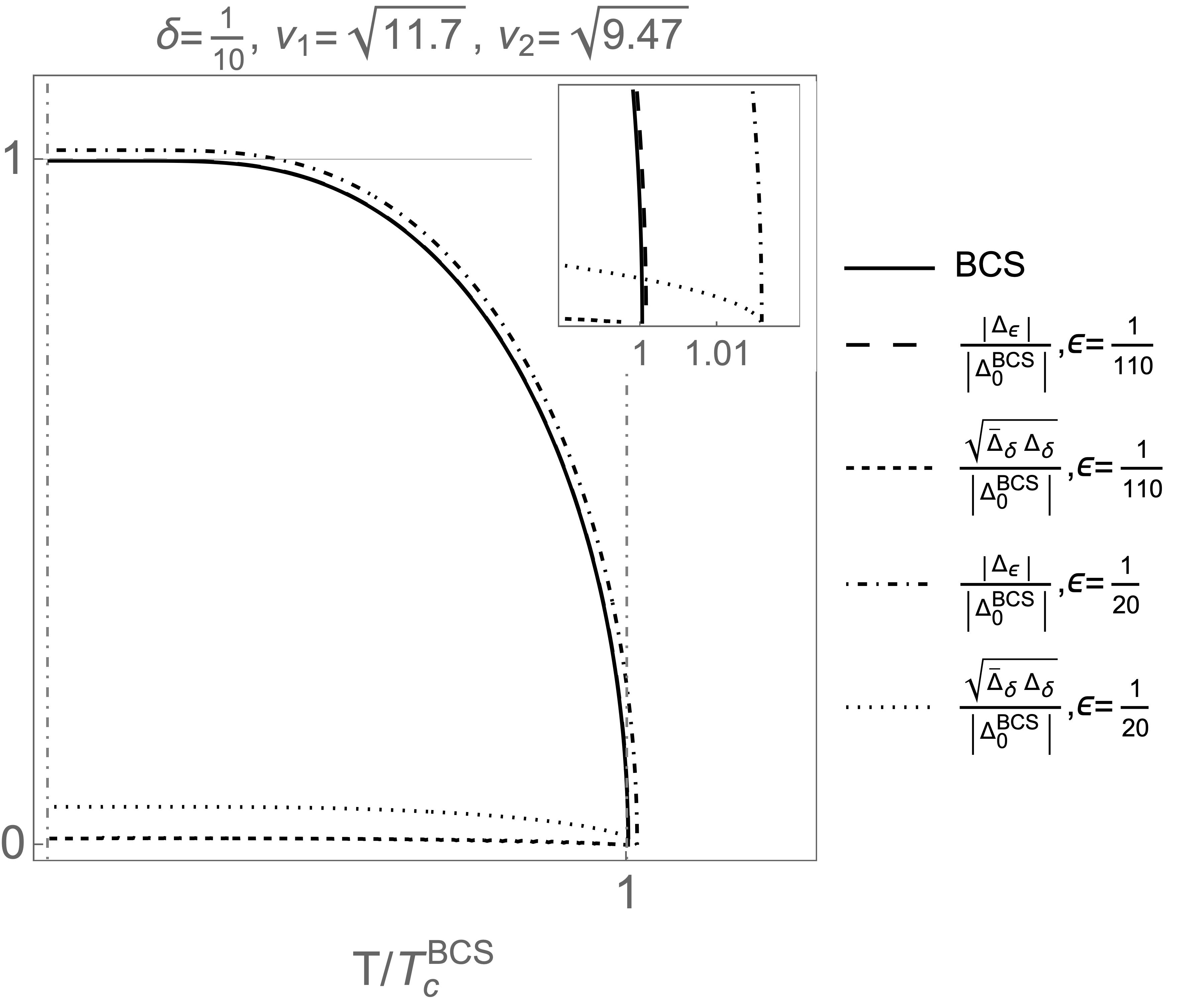
Figure 3: A numerical plot of the gap parameters of the BCS model and our model as a function of temperature. They are obtained from the gap equations $\delta S_{\text{eff}}/\delta\Delta_{1}=0$ and $\delta S_{\text{eff}}/\delta\Delta_{2}=0$ with the approximation $\epsilon\ll\delta\ll 1$ up to, but not including, the order $\delta\epsilon$. Parameters are taken to be $1/g\nu_{1}=1/0.39$, $\nu_{1}=\sqrt{11.7}$, $\nu_{2}=\sqrt{9.47}$, and $\delta=1/10$ with two values $\epsilon=1/20$, $\epsilon=1/110$. Solid and dotted lines are the real and imaginary parts of the solution.

A.1.1 Solutions of gap parameters

Using the relation (42) and Eq. (49) one finds

$$\Delta_{2}=\left[-\delta+i\frac{\epsilon}{\nu}+\mathcal{O}(\epsilon^{2})\right]\Delta_{1}\implies\Delta_{\epsilon}=\left[1+i\delta\epsilon+\frac{\epsilon^{2}}{\nu}+\mathcal{O}(\epsilon^{3})\right]\Delta_{1},$$ (53)

near the critical temperature $T_{c}$. This allows us to expand the gap equation (A.1) and find

$$0 = \frac{1}{g}\left(1-\frac{\epsilon^{2}}{\nu}+\mathcal{O}(\epsilon^{4})\right)-\frac{T}{V}\sum_{n,\vec{p}}\frac{1}{\omega_{n}^{2}+(\epsilon^{(1)}_{\vec{p}})^{2}+|\Delta_{1}|^{2}}$$ (54)

$$-2\left[i\delta\epsilon+\frac{\epsilon^{2}}{\nu}\right]|\Delta_{1}|^{2}\frac{T}{V}\sum_{n,\vec{p}}\frac{1}{\left(\omega_{n}^{2}+(\epsilon^{(1)}_{\vec{p}})^{2}+|\Delta_{1}|^{2}\right)^{2}}+\mathcal{O}(\delta^{4}).$$

This equation has a complex part coming from the $\delta\epsilon$ term. Therefore, one needs to consider the real and the imaginary part of $\overline{\Delta}_{1}\Delta_{1}$ separately to find the complete picture. However, there is one more parameter $\delta$ at our disposal to make a further approximation. Let us assume we cut off the above equation at order $\delta\epsilon$. Since we assume that $\epsilon\ll\delta$, the order $\epsilon^{2}$ must be smaller than $\delta\epsilon$. Therefore the above equation is approximated to the standard BCS gap equation.

$$0=\frac{1}{g}\left(1+\mathcal{O}(\epsilon^{2})\right)-\frac{T}{V}\sum_{n,\vec{p}}\frac{1}{\omega_{n}^{2}+(\epsilon^{(1)}_{\vec{p}})^{2}+|\Delta_{1}|^{2}}.$$ (55)

We can conclude that the gap parameter $\overline{\Delta}_{1}\Delta_{1}$ takes the real value when approximated to the order $\delta\epsilon$. This result is not surprising since weakening the approximation should eventually result in the standard BCS gap parameter. The numerical solution to the above equation is plotted in Fig. 2. The second gap parameter is found by the relation (53)

$$\sqrt{\overline{\Delta}_{2}\Delta_{2}}=\left(-\delta+i\frac{\epsilon}{\nu}\right)|\Delta_{1}|,$$ (56)

where we find that the quantity $\sqrt{\overline{\Delta}_{2}\Delta_{2}}$ has a real and an imaginary part, which is also plotted in Fig. 2.

Lastly, let us make a comment that a better approximation of the complex gap parameters $\{\Delta_{\epsilon},\Delta_{\delta}\}$ or $\{\Delta_{1},\Delta_{2}\}$ requires a higher-order correction to the gap equation. However, our main motivation is to expand the trace log term of the effective action (5) in the main text, which is only allowed when the gap parameters $\Delta_{\epsilon}$ and $\Delta_{\delta}$ are small near the critical temperature. Therefore we do not need to consider the higher order correction to fulfil our main motivation.

Appendix B Consistancy check

From the second equation (22), we find the relation between $\Delta_{1}$ and $\Delta_{2}$

$$\frac{\Delta_{2}}{\Delta_{1}}(T)=\frac{i\epsilon r_{1}-\delta\left\{r_{2}-\frac{1}{g}\frac{\epsilon}{i\delta}\right\}}{r_{2}-\frac{1}{g}\frac{\epsilon}{i\delta}}.$$ (57)

This quantity can be evaluated at the critical temperature by using Eq. (A.1), which gives $r_{1}=r_{2}/\nu=(1-\epsilon^{2}/\nu)/g$ and the above equation is reduced to $\Delta_{2}(T_{c})/\Delta_{1}(T_{c})=-\delta+i\epsilon/\nu+\mathcal{O}(\epsilon^{2})$. This approximation agrees with the relation obtained via the microscopic approach (53).

The first equation can be solved by inserting the solution (57) to the Eq. (21):

$$\overline{\Delta}_{1}\Delta_{1}=-\frac{1}{2u_{1}}\left[r_{1}-\frac{1}{g}+\delta^{2}r_{2}+\delta r_{2}\frac{\Delta_{2}}{\Delta_{1}}\right]\rightarrow-\frac{1}{g2u_{1}}\left[i\delta\epsilon+\mathcal{O}(\epsilon^{2})\right]\text{ as }T\rightarrow T_{c}.$$ (58)

In the previous section, we have cut off the gap equation at the order $\delta\epsilon$ to obtain the real gap parameter. This implies that the quantity $\overline{\Delta}_{1}\Delta_{1}$ vanishes at the critical temperature. Therefore, we have shown the consistency between the microscopic and macroscopic theories up to the order $\delta\epsilon$.

References

[1]
Tosio Kato.
Perturbation theory for linear operators, volume 132.
Springer Science & Business Media, 2013.
[2]
Carl M Bender and Stefan Boettcher.
Real spectra in non-Hermitian Hamiltonians having PT-symmetry.
Physical Review Letters, 80(24):5243, 1998.
[3]
Tamar Goldzak, Alexei A Mailybaev, and Nimrod Moiseyev.
Light stops at exceptional points.
Physical Review Letters, 120(1):013901, 2018.
[4]
WD Heiss, FG Scholtz, and HB Geyer.
The large N behaviour of the Lipkin model and exceptional points.
Journal of Physics A: Mathematical and General, 38(9):1843,
2005.
[5]
Kazuki Yamamoto, Masaya Nakagawa, Kyosuke Adachi, Kazuaki Takasan, Masahito
Ueda, and Norio Kawakami.
Theory of non-Hermitian fermionic superfluidity with a
complex-valued interaction.
Physical Review Letters, 123(12):123601, 2019.
[6]
Ryo Hanai, Alexander Edelman, Yoji Ohashi, and Peter B Littlewood.
Non-Hermitian phase transition from a polariton Bose-Einstein
condensate to a photon laser.
Physical Review Letters, 122(18):185301, 2019.
[7]
WD Heiss.
The physics of exceptional points.
Journal of Physics A: Mathematical and Theoretical,
45(44):444016, 2012.
[8]
Stephan Dürr, Juan José García-Ripoll, Niels Syassen, Dominik M
Bauer, Matthias Lettner, J Ignacio Cirac, and Gerhard Rempe.
Lieb-liniger model of a dissipation-induced tonks-girardeau gas.
Physical Review A, 79(2):023614, 2009.
[9]
Yuto Ashida, Shunsuke Furukawa, and Masahito Ueda.
Quantum critical behavior influenced by measurement backaction in
ultracold gases.
Physical Review A, 94(5):053615, 2016.
[10]
Masaya Nakagawa, Norio Kawakami, and Masahito Ueda.
Non-Hermitian Kondo effect in ultracold alkaline-earth atoms.
Physical Review Letters, 121(20):203001, 2018.
[11]
José A. S Lourenço, Ronivon L Eneias, and Rodrigo G Pereira.
Kondo effect in a PT-symmetric non-Hermitian Hamiltonian.
Physical Review B, 98(8):085126, 2018.
[12]
A. J Daley, J. M Taylor, S Diehl, M Baranov, and P Zoller.
Atomic three-body loss as a dynamical three-body interaction.
Physical Review Letters, 102(4):040402, 2009.
[13]
A. M Begun, Maxim N Chernodub, and A. V Molochkov.
Phase diagram and vortex properties of a PT-symmetric non-Hermitian
two-component superfluid.
Physical Review D, 104(5):056024, 2021.
[14]
Daniel S Kosov, Tomaž Prosen, and Bojan Žunkovič.
Lindblad master equation approach to superconductivity in open
quantum systems.
Journal of Physics A: mathematical and theoretical,
44(46):462001, 2011.
[15]
Ananya Ghatak and Tanmoy Das.
Theory of superconductivity with non-Hermitian and parity-time
reversal symmetric Cooper pairing symmetry.
Physical Review B, 97(1):014512, 2018.
[16]
A Kantian, M Dalmonte, S Diehl, W Hofstetter, P Zoller, and A. J Daley.
Atomic color superfluid via three-body loss.
Physical Review Letters, 103(24):240401, 2009.
[17]
Juan José García-Ripoll, Stephan Dürr, Niels Syassen, Dominik M
Bauer, Matthias Lettner, Gerhard Rempe, and J Ignacio Cirac.
Dissipation-induced hard-core boson gas in an optical lattice.
New Journal of Physics, 11(1):013053, 2009.
[18]
Vladyslav Kozii and Liang Fu.
Non-Hermitian topological theory of finite-lifetime quasiparticles:
prediction of bulk Fermi arc due to exceptional point.
arXiv preprint arXiv:1708.05841, 2017.
[19]
Ryo Hanai and Peter B Littlewood.
Critical fluctuations at a many-body exceptional point.
Physical Review Research, 2(3):033018, 2020.
[20]
Fritz London and Heinz London.
The electromagnetic equations of the supraconductor.
Proceedings of the Royal Society of London. Series
A-Mathematical and Physical Sciences, 149(866):71–88, 1935.
[21]
John Bardeen, Leon N Cooper, and John Robert Schrieffer.
Theory of superconductivity.
Physical Review, 108(5):1175, 1957.
[22]
Andreas Fring and Takanobu Taira.
Goldstone bosons in different PT-regimes of non-Hermitian scalar
quantum field theories.
Nuclear Physics B, 950:114834, 2020.
[23]
Kohei Kawabata, Ken Shiozaki, Masahito Ueda, and Masatoshi Sato.
Symmetry and topology in non-hermitian physics.
Physical Review X, 9(4):041015, 2019.
[24]
Philip D Mannheim.
Goldstone bosons and the Englert-Brout-Higgs mechanism in
non-Hermitian theories.
Physical Review D, 99(4):045006, 2019.
[25]
Andreas Fring and Takanobu Taira.
Massive gauge particles versus Goldstone bosons in non-Hermitian
non-Abelian gauge theory.
The European Physical Journal Plus, 137(6):1–15, 2022.
[26]
Jean Alexandre, Peter Millington, and Dries Seynaeve.
Symmetries and conservation laws in non-Hermitian field theories.
Physical Review D, 96(6):065027, 2017.
[27]
H Suhl, BT Matthias, and LR Walker.
Bardeen-Cooper-Schrieffer theory of superconductivity in the case of
overlapping bands.
Physical Review Letters, 3(12):552, 1959.
[28]
Kazuki Yamamoto, Masaya Nakagawa, Naoto Tsuji, Masahito Ueda, and Norio
Kawakami.
Collective excitations and nonequilibrium phase transition in
dissipative fermionic superfluids.
Physical Review Letters, 127(5):055301, 2021.
[29]
Vittorio Gorini, Andrzej Kossakowski, and Ennackal Chandy George Sudarshan.
Completely positive dynamical semigroups of -level systems.
Journal of Mathematical Physics, 17(5):821–825, 1976.
[30]
Goran Lindblad.
On the generators of quantum dynamical semigroups.
Communications in Mathematical Physics, 48(2):119–130, 1976.
[31]
Anne-Maria Visuri, Jeffrey Mohan, Shun Uchino, Meng-Zi Huang, Tilman Esslinger,
and Thierry Giamarchi.
Dc transport in a dissipative superconducting quantum point contact.
arXiv preprint arXiv:2304.00928, 2023.
[32]
Chen-How Huang, Thierry Giamarchi, and Miguel A Cazalilla.
Modeling particle loss in open systems using keldysh path integral
and second order cumulant expansion.
arXiv preprint arXiv:2305.13090, 2023.
[33]
Heinz-Peter Breuer, Francesco Petruccione, et al.
The theory of open quantum systems.
Oxford University Press on Demand, 2002.
[34]
M Naghiloo, M Abbasi, Yogesh N Joglekar, and KW Murch.
Quantum state tomography across the exceptional point in a single
dissipative qubit.
Nature Physics, 15(12):1232–1236, 2019.
[35]
Chang Liu, Zhe-Yu Shi, and Ce Wang.
Weakly interacting bose gas with two-body losses.
arXiv preprint arXiv:2209.10427, 2022.
[36]
Yosuke Takasu, Tomoya Yagami, Yuto Ashida, Ryusuke Hamazaki, Yoshihito Kuno,
and Yoshiro Takahashi.
PT-symmetric non-Hermitian quantum many-body system using ultracold
atoms in an optical lattice with controlled dissipation.
Progress of Theoretical and Experimental Physics,
2020(12):12A110, 2020.
[37]
M Atala, M Aidelsburger, M Lohse, JT Barreiro, B Paredes, and I Bloch.
Observation of the meissner effect with ultracold atoms in bosonic
ladders.
arXiv preprint arXiv:1402.0819, 2014.
[38]
Daniel Cano, B Kasch, Helge Hattermann, Reinhold Kleiner, Claus Zimmermann,
Dieter Koelle, and József Fortágh.
Meissner effect in superconducting microtraps.
Physical review letters, 101(18):183006, 2008.
[39]
Pierre-Gilles De Gennes and Philip A Pincus.
Superconductivity of metals and alloys.
CRC Press, 2018.
[40]
Jean Alexandre, John Ellis, Peter Millington, and Dries Seynaeve.
Spontaneous symmetry breaking and the Goldstone theorem in
non-Hermitian field theories.
Physical Review D, 98(4):045001, 2018.
[41]
Andreas Fring and Takanobu Taira.
’t Hooft-Polyakov monopoles in non-Hermitian quantum field theory.
Physics Letters B, 807:135583, 2020.