DyNCA: Real-time Dynamic Texture Synthesis
Using Neural Cellular Automata

Abstract

Current Dynamic Texture Synthesis (DyTS) models can synthesize realistic videos. However, they require a slow iterative optimization process to synthesize a single fixed-size short video, and they do not offer any post-training control over the synthesis process. We propose Dynamic Neural Cellular Automata (DyNCA), a framework for real-time and controllable dynamic texture synthesis. Our method is built upon the recently introduced NCA models and can synthesize infinitely long and arbitrary-sized realistic video textures in real time. We quantitatively and qualitatively evaluate our model and show that our synthesized videos appear more realistic than the existing results. We improve the SOTA DyTS performance by $2\sim 4$ orders of magnitude. Moreover, our model offers several real-time video controls including motion speed, motion direction, and an editing brush tool. We exhibit our trained models in an online interactive demo that runs on local hardware and is accessible on personal computers and smartphones.

Figure 1: Our DyNCA model can synthesize infinitely-long realistic dynamic texture videos with arbitrary size in real time. Target Appearance: DyNCA learns a desired texture pattern from a given target appearance image. Target Dynamics: DyNCA can learn motion from different target sources. We allow the users to define the desired motion either by a hand-crafted optical-flow imageor a dynamic texture video. Synthesized Result: DyNCA synthesizes realistic dynamic texture videos. Each synthesized video frame resembles the target appearance, while the concatenation of frames induces the motion of the target dynamics. See our real-time interactive demo at.

1 Introduction

Textures are everywhere. We perceive them as spatially repetitive patterns. Dynamic Textures are textures that change over time and induce a sense of motion. Flames, sea waves, and fluttering branches are everyday examples. Understanding and computationally modeling dynamic textures is an intriguing problem, as these patterns are observed in most natural scenes.

The goal of Dynamic Texture Synthesis (DyTS) [7, 6, 23, 10, 12, 5, 8, 24, 32, 27, 29] is to generate perceptually-equivalent samples of an exemplar video texture. Applications of DyTS include the creation of special effects for backdrops and video games [21], dynamic style transfer [24], and creating cinemagraphs [12].

The state-of-the-art (SOTA) dynamic texture synthesis methods [24, 27, 32, 8, 29] follow the same trend. They aim to find better optimization strategies to iteratively update a randomly initialized video until the synthesized video resembles the exemplar dynamic texture. Although the SOTA methods are able to synthesize acceptable quality videos, their optimization process is very slow and requires several hours to generate a single fixed-resolution short video on a high-end GPU. Moreover, these methods do not offer any post-training control over the synthesized video.

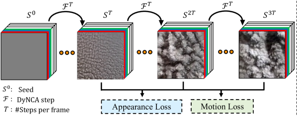
Figure 2: Overview of DyNCA. Starting from a seed state, DyNCA iteratively updates it, generating an image sequence. We extract images from this sequence and compare them with an appearance target as well as a motion target to obtain the DyNCA training objectives. After training, DyNCA can adapt to seeds of different heights and widths, and synthesize videos with arbitrary lengths. Sequentially applying DyNCA updates on the seed synthesizes dynamic texture videos in real time.

In this paper we propose Dynamic Neural Cellular Automata (DyNCA), a model for dynamic texture synthesis that is fast to train, and once trained, can synthesize infinitely-long, arbitrary-resolution dynamic texture videos in real time on a low-end GPU. Moreover, our method enables several real-time video editing controls, including motion direction and motion speed. Through quantitative and qualitative analysis we demonstrate that our synthesized videos achieve better quality and realism than the previous results in the literature.

Our model builds upon the recently introduced Neural Cellular Automata (NCA) model [18, 19]. While Niklasson et al. [19] train the NCA with the goal of synthesizing static textures only, the NCA model is able to spontaneously generate randomly moving patterns. As an inherent property of NCA, these spontaneous motions are, however, unstructured and uncontrolled. We modify the architecture and the training scheme of NCA so that it can learn to synthesize video textures that have the desired motion and appearance.

In short, our DyNCA model acts as a stochastic Partial Differential Equation (PDE), parameterized by a small neural network. DyNCA starts from a constant initial state called seed, and then iteratively evolves the state according to its trainable PDE update rule to generate a sequence of images. This image sequence is then evaluated against the appearance exemplar and the motion target to calculate the loss functions for the optimization of DyNCA, as illustrated in Figure 2. We allow the user to specify the desired motion either by a motion vector field or an exemplar dynamic texture video. Moreover, by using a different target for the appearance and the motion, our model can perform dynamic style transfer, as shown in Figure 1. Our contributions summarized are:

• Our DyNCA model, once trained, can synthesize dynamic texture videos in real time.

• Our synthesized videos are on-par with or even better than the existing results in terms of realism and quality.

• After training, our DyNCA model can synthesize infinitely-long videos with arbitrary frame sizes.

• Our DyNCA framework enables several real-time interactive video editing controls including speed, direction, a brush tool, and local coordinate transformation.

• We can perform real-time dynamic style transfer by learning appearance and motion from distinct sources.

2 Related Works

In the following section, we discuss the existing DyTS methods. For comparison, Table 1 summarizes the strengths (✓) and shortcomings (✗) of these methods.

2.1 Dynamic Texture Synthesis

In the literature, there are two dominant techniques to synthesize dynamic texture videos. Recent approaches follow the seminal work of Gatys et al.[9] for texture synthesis. The authors propose an optimization-based method that relies on the features extracted by a deep neural network trained for image classification. Gatys et al.[9] show that the Gram matrices of features extracted by the VGG network [22] capture the perceptual qualities of texture images. Funke et al.[8] extend Gatys’s idea to dynamic texture synthesis, and use a cross-frame Gram matrix of VGG features to capture the temporal characteristics of dynamic textures. Tesfaldet et al.[24] and Zhang et al. [32] use a pre-trained optical flow network for extracting the motion features, which allows them to disentangle the appearance and motion aspects of video textures. Xie et al.[27] use an energy-based model characterized by a spatio-temporal 3D ConvNet and synthesize textures by sampling using Langevin dynamics.

These methods utilize the expressivity of neural networks to produce realistic high-quality dynamic texture videos. However, they require a long training time to synthesize a single short video. Moreover, none of these methods provide any post-training controls over motion speed, frame size, and motion direction. These shortcomings make these methods unsuitable for real-time applications.

Earlier DyTS methods that can potentially enable real-time synthesis utilized PDEs to model dynamic textures [6, 5, 31, 10, 30]. To synthesize video textures, Doretto et al.[6] propose to use a linear dynamical system (LDS) in which each frame of the video is controlled by a latent variable whose evolution through time is driven by random noise. The latent variable is obtained via projection of the target texture image into a lower dimensional space by singular value decomposition (SVD). Costantini et al. [5] propose to use higher-order SVD to improve the expressivity of LDS-based models. Yuan et al.[31] introduce feedback into the LDS to improve the stability of the dynamical system. All these methods can synthesize new video textures without re-training, and potentially in real time. However, the synthesized videos are of low quality and contain artifacts.

Method	A	B	C	D	E	F	G
Costantini et al. [5]	✗	✓	✓	✗	✓	✗	✗
Doretto et al. [6]	✗	✓	✓	✗	✓	✗	✗
Funke et al. [8]	✗	✓	✗	✗	✗	✗	✗
Tesfaldet et al. [24]	✗	✓	✗	✗	✗	✓	✓
Xie et al. [27]	✗	✗	✗	✗	✓	✗	✗
Zhang et al. [32]	✗	✓	✗	✗	✗	✓	✓
DyNCA (Ours)	✓	✓	✓	✓	✗	✓	✓

Table 1: Comparison of DyTS methods. (A) Can synthesize videos with arbitrary frame size after training. (B) Can synthesize arbitrarily long videos. (C) Can synthesize new video samples without re-training. (D) Allows real-time video editing (speed, direction, and a brush tool). (E) Does not rely on pre-trained models to extract motion or texture information. (F) Has disentangled appearance and motion. (G) Can learn motion from vector fields.

Our DyNCA method benefits from the best of both approaches by combining the expressivity of neural networks with PDEs. Having $2\sim 4$ orders of magnitude fewer parameters than the SOTA models, our model can synthesize realistic dynamic texture videos in real time.

2.2 NCA for Texture Synthesis

Gilpin [11] shows that Cellular Automata models can be represented using Convolutional Neural Networks. Extending [11], Mordvinstev et al. [18] propose the Neural Cellular Automata model and show its potential in creating various self-organizing systems [18, 17, 20, 19]. NCA is inspired by Turing’s seminal work [25] on pattern generation, and the observation that many natural patterns stem from local interactions between tiny particles, cells, or molecules [19].

Niklasson et al.[19, 17] were the first to train NCA models to synthesize textures. While the NCA training signal originates from a static exemplar texture image, the model is able to spontaneously generate stable but randomly moving textures. We modify the architecture and training scheme of NCA to enable synthesizing structured motion. First, our DyNCA model receives supervision from a pre-trained optical-flow network, which enables it to synthesize a video texture with structured motion. Moreover, we incorporate multi-scale perception and positional encoding into the DyNCA architecture. The proposed architectural changes increase the communication range of the cells and allow the cells to be aware of global information, respectively.

3 DyNCA Architecture

In the following sections, we first review the NCA model and then present the architecture of our DyNCA.

3.1 Neural Cellular Automata (NCA)

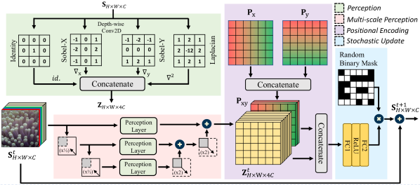
Figure 3: Illustration of a single DyNCA step. Given an input state $\mathbf{S}^{t}\in R^{H\times W\times C}$ at time step $t$, each cell first perceives its neighbors on various scales with the same perception layer. The perception tensor of each scale is then upsampled and summed up, and is concatenated with the positional encoding tensor $\mathbf{P}_{\textup{x}\textup{y}}$. Each cell then applies the same update rule, parameterized by a small MLP. Finally, all cells perform a stochastic residual update to determine the state of the cells in time $t+\Delta t$. We use $\Delta t=1$ in our model.

The idea of NCA stems from cellular automata, in which cells live on a grid, and each cell communicates with its neighbors to determine the cell’s next state. In NCA, cell states at time $t$ are represented by $\mathbf{S}^{t}\in\mathbb{R}^{H\times W\times C}$ where $H\times W$ is the grid size. The $C$ dimensional vector $s^{t}_{ij}$ encodes the state of the cell at location $i,j$, where the first three dimensions define the RGB color of the cell.

The NCA starts from a constant zero-filled initial state called seed and evolves this state over time according to its trainable PDE. The update rule of this PDE consists of two parts, Perception and Stochastic Update. At the perception stage, each cell gathers information from its surrounding neighbors, forming the perception vector $z_{ij}\in\mathbb{R}^{4C}$, illustrated in the green box in Figure 3.

$$z_{ij}=Concat(s_{ij},\nabla_{\textup{x}}\mathbf{S}|_{ij},\nabla_{\textup{y}}\mathbf{S}|_{ij},\nabla^{2}\mathbf{S}|_{ij})$$ (1)

Note that the convolution kernels in the perception stage are frozen during training. In the stochastic update stage, the new state of each cell is determined based on its perception vector. The update stage of NCA can be viewed as a stochastic discrete-time, discrete-space PDE:

$$\begin{split}\mathbf{S}&{}^{t+1}=\mathcal{F}(\mathbf{S}^{t})=\mathbf{S}^{t}+\frac{\partial\mathbf{S}}{\partial t}\Delta t\\ &\frac{\partial s_{ij}}{\partial t}=\textup{MLP}(z_{ij})\odot M\end{split}$$ (2)

where MLP is a Multi Layered Perceptron with two layers and a ReLU activation function. The residual update values produced by the MLP are multiplied by a binary random variable $M$ to introduce stochasticity into the model. This ensures that the cells can work asynchronously, and also enables synthesizing new texture samples. The stochastic update stage is illustrated in the blue box in Figure 3.

To facilitate long-range cell communication and to allow the cells to be aware of global information, we introduce multi-scale perception and positional encoding into the vanilla NCA architecture, respectively. Our experiments in section 5 demonstrate their necessity for DyTS. The overall architecture of our DyNCA model is illustrated in Figure 3. To the best of our knowledge, we are the first to incorporate these two architectural changes in conjunction with NCA models. In the following sections, we elaborate on the proposed architectural modifications.

3.2 Multi-scale Perception

In the perception stage of vanilla NCA, each cell only receives information from its eight surrounding cells. Therefore, many timesteps are needed for far-apart cells to perceive and communicate with each other. This problem becomes more pronounced when we increase the grid size $H\times W$, since the $3\times 3$ perception kernels become smaller in proportion to the image size. One straightforward solution is to increase the number of NCA steps during training to facilitate long-range cell communication. However, this simple solution increases memory usage, slows down the training, and makes the training more unstable.

To solve this problem, we propose Multi-Scale Perception (MSP). The idea of using multi-scale analysis predates deep learning and has shown its effectiveness in many computer vision tasks [1, 14, 3, 15]. We build a pyramid of cell states via bilinear downsampling and apply the same perception kernels at different scales. To combine the information from all scales, we upsample and sum up the perception vectors, as shown in the red box in Figure 3. Multi-scale perception increases the communication range of the cells and allows messages to pass between faraway cells in fewer steps. It also improves the stability of DyNCA and makes the training less sensitive to hyperparameters. We perform an ablation study of multi-scale perception in section 5.4 and show its importance in preserving appearance fidelity.

3.3 Positional Encoding

In order to apply the $3\times 3$ depth-wise convolutions in the perception stage, one needs to adopt a padding strategy to retain the spatial dimensions. Niklasson et al. [19] use circular padding to make the cells homogeneous and to reduce spatial inductive bias. While cell homogeneity is a good assumption for generating static textures, it is not suitable for synthesizing structured motion. Our intuition is that, in physical systems, motion not only arises from local interactions between tiny particles and cells, but also from global external forces such as gravity. Hence, we allow the cells to be aware of their position and propose to use replicate padding and Cartesian Positional Encoding (CPE), which is known to provide a more consistent spatial inductive bias than zero-padding [28]. As illustrated in the purple box in Figure 3, we concatenate the output of the multi-scale perception stage with a two-channel tensor $\mathbf{P}_{\textup{xy}}$, where $\mathbf{P}_{ij}=\begin{bmatrix}\frac{2i+1.0}{W}\\ \frac{2j+1.0}{H}\end{bmatrix}-1.0$. Our ablation study in section 5.4 shows that employing CPE drastically improves motion consistency and accuracy in the synthesized videos.

4 DyNCA Training

Our DyNCA model acts as a PDE and generates a sequence of images $\mathcal{I}^{g}=\{\mathcal{I}^{g}_{1},\mathcal{I}^{g}_{2},...\}$. We sample the synthesized video frames $\mathcal{V}^{g}=\{\mathcal{V}^{g}_{1},\mathcal{V}^{g}_{2},...\}$ from this image sequence by mapping $T$ DyNCA steps to one frame, i.e. $\mathcal{V}^{g}_{k}=\mathcal{I}^{g}_{kT}$. The synthesized video is then evaluated against the target appearance and the target motion to compute the appearance loss $\mathcal{L}_{appr}$ and the motion loss $\mathcal{L}_{motion}$, respectively. This process is shown in Figure 2. Our final loss is $\mathcal{L}_{\textup{DyNCA}}=\mathcal{L}_{appr}+\lambda\mathcal{L}_{motion}$. The overall scheme of the proposed loss functions is illustrated in Figure 4.

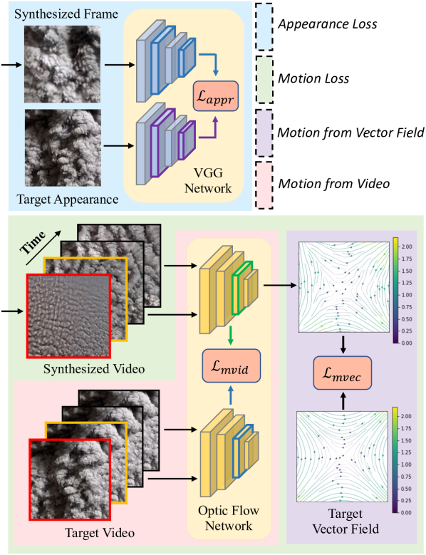
Figure 4: Overview of our loss functions. Appearance loss ($\mathcal{L}_{appr}$): DyNCA learns the target appearance from a static image via minimizing an optimal-transport-based style matching loss [13] between deep features extracted from the VGG16 network [22]. Motion Loss ($\mathcal{L}_{mvec}$): We guide DyNCA to synthesize a video having an optical flow similar to the target vector field. Motion Loss ($\mathcal{L}_{mvid}$): DyNCA fits the target video motion by minimizing an optimal-transport-based style matching loss between deep features of a pre-trained optical-flow prediction network.

4.1 Appearance Loss

We follow the texture fitting scheme proposed by Niklasson et al.[19], where the statistics of deep features of the NCA-generated images are forced to match the ones of the target texture. We use a pre-trained VGG16 network [22] to extract the deep features from the images. We denote VGG as $\mathcal{F}_{VGG}$ and the feature map extracted from layer $l$ as $\mathcal{F}^{l}_{VGG}$. Niklasson et al. [19] use the Gram matrix to define the training objective of the NCA. However, using Gram matrices can cause unstable training[26], and can result in textures with wrong colors [16, 19]. Hence, we use the style loss proposed by Kolkin et al.[13], which has shown to produce better results. This loss is composed of a structure-matching term and a moment-matching term. Given a feature map of size $C\times H\times W$, the algorithm first creates a set of deep features with $n=H\times W$ elements by flattening the feature map along the spatial dimensions. Let $X$ and $Y$ be the deep feature set of a synthesized image and target appearance image, respectively. Then the structure-matching term $\mathcal{L}_{s}$ and the moment-matching term $\mathcal{L}_{m}$ are defined as:

$$\begin{split}D(&A,B)=\frac{1}{|A|}\sum_{i}\mathop{min}\limits_{j}\left(1-\frac{A_{i}\cdot B_{j}}{||A_{i}||_{2}||B_{j}||_{2}}\right)\\ &\mathcal{L}_{s}(X,Y)=max\left\{D(X,Y),D(Y,X)\right\},\end{split}$$ (3)

$$\mathcal{L}_{m}(X,Y)=\frac{1}{C}\left\|\boldsymbol{\mu}_{X}-\boldsymbol{\mu}_{Y}\right\|_{1}+\frac{1}{C^{2}}\left\|\boldsymbol{\Sigma}_{X}-\boldsymbol{\Sigma}_{Y}\right\|_{1},$$ (4)

where $D$ measures the distance between two deep feature sets, and $\boldsymbol{\mu}$, $\boldsymbol{\Sigma}$ are the mean and covariance matrix of their corresponding set, respectively. Let $X^{l}_{k}$ and $Y^{l}$ be deep VGG features extracted by $\mathcal{F}^{conv\;l\_1}_{VGG}$, where $l$ and $k$ indicate the VGG block index and the synthesized image index, respectively. Our final appearance loss is then defined as:

$$\mathcal{L}_{appr}=\frac{1}{K}\sum^{K}_{k=1}\sum^{5}_{l=1}\left(\mathcal{L}_{s}(X^{l}_{k},Y^{l})+\mathcal{L}_{m}(X^{l}_{k},Y^{l})\right)$$ (5)

4.2 Motion Loss

The motion loss guides the DyNCA to produce the desired motion. We use the pre-trained Optical-Flow Prediction Network from [24] to quantify the motion information between two frames. We denote this network as $\mathcal{F}_{OF}$, and the feature map extracted from layer $l$ as $\mathcal{F}^{l}_{OF}$. For different types of target motion sources, namely vector fields and videos, our motion loss takes two different forms, $\mathcal{L}_{mvec}$ and $\mathcal{L}_{mvid}$, respectively. These terms are discussed below.

4.2.1 Motion from Vector Field

Let $U^{t}\in\mathbb{R}^{H\times W\times 2}$ be the target motion vector field. Let $U^{g}=\mathcal{F}_{OF}(\mathcal{I}^{g}_{t_{1}},\mathcal{I}^{g}_{t_{2}})$ be the optical-flow prediction on two synthesized images, where $t_{1},t_{2}$ are two random indices such that $t_{2}>t_{1}$. We propose two losses, $\mathcal{L}_{dir}$ for matching the motion direction, defined as:

$$\mathcal{L}_{dir}=\frac{1}{HW}\sum_{i,j}\left(1-\frac{U^{g}_{ij}\cdot U^{t}_{ij}}{\left\|U^{g}_{ij}\right\|_{2}\left\|U^{t}_{ij}\right\|_{2}}\right),$$ (6)

and $\mathcal{L}_{norm}$ for matching the motion magnitude, defined as:

$$\mathcal{L}_{norm}=\frac{1}{HW}\sum_{i,j}\left|\frac{T}{t_{2}-t_{1}}\left\|U^{g}_{ij}\right\|_{2}-\left\|U^{t}_{ij}\right\|_{2}\right|.$$ (7)

Since $t_{1},t_{2}$ are selected randomly, we scale the norm of the $U^{g}$ by $\frac{T}{t_{2}-t_{1}}$ before comparing it against the target motion vector field. We define our final loss $\mathcal{L}_{mvec}$ as:

$$\mathcal{L}_{mvec}=\left(1.0-min\{1.0,\mathcal{L}_{dir}\}\right)\mathcal{L}_{norm}+\gamma\mathcal{L}_{dir},$$ (8)

where $\gamma$ is a constant coefficient. We set the norm-matching loss weight to $\left(1.0-min\{1.0,\mathcal{L}_{dir}\}\right)$ to guide the training process to first focus on producing motion with the correct direction before trying to match the norm of the synthesized motion with the target vector field.

4.2.2 Motion from Video

For training DyNCA to learn the motion from a target video, we aim to match the motion between successive frames of the synthesized and target videos. We synthesize a video $\mathcal{V}^{g}$ with $K$ frames, and randomly pick the same number of consecutive frames from the target video, forming $\mathcal{V}^{t}$. Inspired by Tesfaldet et al. [24], we feed successive video frames to a pre-trained optical-flow network and extract deep features from the concatenation layer of the network, denoted as $\mathcal{F}^{concat}_{OF}$. To compare the deep optical flow features of the target and the synthesized videos, we use the same structure-matching and moment-matching terms defined in Section 4.1. We denote the extracted deep optical-flow features as $X_{k}$ for the synthesized video, and $Y_{k}$ for the target video, where $k$ indicates the frame index. Notice that there are $K-1$ successive frame pairs in total. We define the objective for learning motion from video textures as:

$$\mathcal{L}_{mvid}=\frac{1}{K-1}\sum^{K-1}_{k=1}\left(\mathcal{L}_{s}(X_{k},Y_{k})+\mathcal{L}_{m}(X_{k},Y_{k})\right)$$ (9)

5 Experiments

Target Appearance		Target Dynamics (Motion)			Synthesized Result
		Video		Optical Flow	Video		Optical Flow
Dynamic Texture Synthesis			$\overset{OF}{{\color[rgb]{0,0,0}\Longrightarrow}}$			$\overset{OF}{{\color[rgb]{0,0,0}\Longrightarrow}}$
			$\overset{OF}{{\color[rgb]{0,0,0}\Longrightarrow}}$			$\overset{OF}{{\color[rgb]{0,0,0}\Longrightarrow}}$
Dynamic Style Transfer			$\overset{OF}{{\color[rgb]{0,0,0}\Longrightarrow}}$			$\overset{OF}{{\color[rgb]{0,0,0}\Longrightarrow}}$
			$\overset{OF}{{\color[rgb]{0,0,0}\Longrightarrow}}$			$\overset{OF}{{\color[rgb]{0,0,0}\Longrightarrow}}$

Figure 5: Results of dynamic texture synthesis and dynamic style transfer with DyNCA-L-$256^{2}$. Dynamic Texture Synthesis: DyNCA faithfully reproduces the target appearance and target dynamics. Dynamic Style Transfer: DyNCA can learn appearance and motion from different sources. Note that DyNCA does not simply copy the target dynamics from the video, but learns the style of the given motion and naturally adapts it to the target appearance, as shown by the optical-flow images. See our real-time interactive demo https://dynca.github.io

We conduct experiments on the critical parameters of DyNCA, including $N_{C},N_{H},N_{W},N_{FC}$, where $N_{C},N_{H},N_{W}$ are the size of the DyNCA seed state and $N_{FC}$ is the output dimensionality of the first layer of MLP in DyNCA. Concretely, we set $N_{C}=12,N_{FC}=96$ for DyNCA-S and $N_{C}=16,N_{FC}=128$ for DyNCA-L. Although DyNCA can adapt to arbitrary seed sizes after training, the seed resolution used during training affects the texture details. We experiment with both $128^{2}$ and $256^{2}$ spatial resolutions for the seed. We use Positional Encoding for all of the DyNCA configurations, and enable Multi-Scale Perception only when training with the $256\times 256$ seed size. Table 2 summarizes the DyNCA configurations. We perform our experiments on an Nvidia-A100 GPU, and use Adam optimizer with an initial learning rate of 0.001. We refer the reader to the supplementary for further training details.

5.1 Dynamic Texture Synthesis

Method	Res.	Training Time (s)	Synthesis Time (s)	# Parameters
A [24]	$256^{2}$	#frames $\times$ 500	$5.0\times 10^{2}$	#frames $\times$ 0.2M
B [27]	$224^{2}$	#frames $\times$ 400	$4.0\times 10^{2}$	81M
C [27]	$100^{2}$	#frames $\times$ 8.5	$8.5\times 10^{0}$	2.8M
DyNCA-S	$128^{2}$	2320	$3.3\times 10^{-2}$	0.006M
DyNCA-S	$256^{2}$	3980	$5.7\times 10^{-2}$	0.006M
DyNCA-L	$128^{2}$	2370	$3.5\times 10^{-2}$	0.010M
DyNCA-L	$256^{2}$	4380	$5.7\times 10^{-2}$	0.010M

Table 2: Comparison of training time, synthesis time per frame, and number of trainable parameters of different DyTS methods. (A) Tesfaldet et al. [24]; (B) Xie et al. [27] FC config; (C) Xie et al. [27] ST config. For (B) and (C), training and synthesis happen simultaneously, and the video is synthesized once the training is finished. All methods are evaluated on a single A100 40GB GPU.

Figure 6: Results of DyNCA trained on various target vector fields as the motion target. First and second row: Symbolic and colored optical-flow representations of the target vector fields. Third row: Snapshot of the optical-flow estimations of the videos synthesized by DyNCA-S-$128^{2}$. The target appearance used for training the model is fibrous_0145 texture from the DTD dataset [4].

We present the results of synthesizing dynamic textures using DyNCA, where the target motion is either a vector field or a video, and the target appearance is a static image.

Motion from Vector Field: We manually design 12 target vector fields, and for each target motion, we train both DyNCA-S and DyNCA-L configurations on 45 different target appearances. We provide the resulting 1080 trained models in our real-time interactive demo. We set seed size to $128\times 128$ and $T=24$, assuming that 24 steps of DyNCA update equals one frame of the synthesized video. Figure 6 shows the optical flow of the DyNCA-S synthesized videos and the corresponding target vector fields used for training.

Motion from Video. We train DyNCA to match the target motion from videos. For the target appearance image, we use one of the video frames or a stylistic image, to perform dynamic texture synthesis and dynamic style transfer, respectively. We train both DyNCA-S and DyNCA-L on 59 target dynamic texture videos provided in [24], setting seed size to $256\times 256$ and $T=64$. Figure 5 provides some visual results. More results are provided in our demo and supplementary. In Table 2, we compare our DyNCA and the previous SOTA models [24, 27] in terms of the computational costs, namely performance and the number of parameters. Note that our DyNCA model is orders of magnitude more efficient in both training and synthesis time as well as the number of parameters. We refer the reader to the supplementary material for the detailed experimental setup.

5.2 Real-time Video Editing

DyNCA can also perform real-time video editing by utilizing the post-training NCA controls introduced in [19]. These edits include direction control, speed control, a brush tool, and local coordinate transformations. We refer the reader to our online demo at https://dynca.github.io for real-time and interactive visualization and experimentation.

Direction Control: By rotating the Sobel convolution kernels $\nabla_{\textup{x}}$ and $\nabla_{\textup{y}}$ in the perception stage, we can control the direction of the motion in the synthesized video. This is done by replacing $\nabla_{\textup{x}}$ and $\nabla_{\textup{y}}$ with $\nabla_{\textup{u}}$ and $\nabla_{\textup{v}}$, where $\binom{\textup{u}}{\textup{v}}=\textup{R}_{\theta}\binom{\textup{x}}{\textup{y}}$ and $\textup{R}_{\theta}$ is the rotation matrix with angle $\theta$. We also rotate $\textup{P}_{\textup{x}\textup{y}}$ by angle $\theta$ so that the position-dependent part of the motion magnitude also rotates accordingly.

Speed Control: We control the speed of the synthesized video by increasing/decreasing $T$, which determines how many DyNCA steps are used to synthesize one video frame.

Brush Tool: The brush tool allows the users to delete pixels from the video. Since our DyNCA model exhibits the self-organization property of the original NCA [19], the model can reorganize itself and continue synthesizing realistic videos by naturally filling the deleted pixels.

Local Coordinate Transformation: DyNCA can create complex motion transformations by allowing each cell to use a different rotation angle $\theta(i,j)$ for transforming its Sobel convolution kernels. For example, setting the rotation angle for the cell at location $(i,j)$ to $arctan\left(\frac{i-\frac{W}{2}}{j-\frac{H}{2}}\right)$ will transform a rightward motion into a circular motion.

5.3 User Study

Although it is tempting to use a metric, e.g. the Gram matrix difference [9], to compare the quality of the videos synthesized by different methods, the variety of training objectives used in the existing methods makes such comparisons biased and unfair. Therefore, we conduct a similar user study as Tesfaldet et al. [24] to quantitatively evaluate and compare the realism of the videos. We show a pair of videos to the participants and ask them to choose the video that appears more realistic. We compare the videos synthesized by (DyNCA, [24], [27]) with each other and also with real videos using the same 59 dynamic texture videos as Tesfaldet et al. [24]. Table 3 shows the results of our user study. Each entry shows the percentage of times that the video from the corresponding column was chosen over the video from the corresponding row. Our method outperforms the other DyTS method in realism. We refer the reader to our supplementary for more details on the user study.

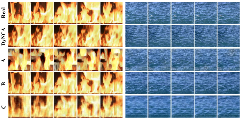
(a)

	Real	DyNCA	A [24]	B [27]	C [27]
Real	N/A	27%	26%	24%	8%
DyNCA	73%	N/A	40%	46%	20%
A [24]	74%	60%	N/A	52%	25%
B [27]	76%	54%	48%	N/A	15%
C [27]	92%	80%	75%	85%	N/A

(b)

Table 3: Top: Comparison of real and synthesized video frames from different methods: (A) Tesfaldet et al. [24]; (B) Xie et al. [27] FC config; (C) Xie et al. [27] ST config. Bottom: Pair-wise comparison results from our user study. The participants see two videos one after another in random order and are asked to choose the video that appears more realistic. Our DyNCA achieves an on-par “fooling” rate when compared with real videos. Yet, our synthesized videos look more realistic when compared to existing DyTS methods (60%, 54%, 80%). All error margins are $\leq 2\%$.

5.4 Ablation Study

Positional Encoding: We ablate the Cartesian Positional Encoding (CPE) and train DyNCA-S-$128^{2}$ with different padding strategies for comparison. In Table 4, we report the average of $\mathcal{L}_{dir}$ and $\mathcal{L}_{norm}$ losses on 4 target vector fields (Diverge, Converge, Circular, and Hyperbolic shown in the last 4 columns of Figure 6) and 10 different target appearances. The results demonstrate that CPE is a necessary component for DyNCA to learn the motion from a structured target vector field, in which the motion direction and magnitude are position-dependent. We show the importance of CPE for video motion fitting in the supplementary.

Multi-Scale Perception:. MSP is key to enable training DyNCA with larger seed sizes. We train DyNCA-L-$256^{2}$ both with and without multi-scale perception and evaluate the results qualitatively and quantitatively. Figure 8 shows the corresponding synthesized video frames, qualitatively demonstrating that single-scale perception causes artifacts to appear in the synthesized frames. We also perform a quantitative evaluation in the supplementary, showing that training with multi-scale perception improves both the appearance $\mathcal{L}_{appr}$ and the video motion $\mathcal{L}_{mvid}$ losses.

6 Limitations

DyNCA has certain limitations. In the case of vector field motion, it cannot generate a correct motion when the target appearance and the target motion are not compatible. For example, DyNCA fails to move a 45-degree oblique-line pattern in a circular manner. For video motion, we find it difficult to automatically set the motion loss weight $\lambda$. Moreover, DyNCA cannot generate diverse motion when the target videos are violating the underlying assumption of dynamic textures, i.e. when they are not temporally homogeneous. In these cases, DyNCA suffers from overfitting to the dominant direction of the motion in the target videos We refer to our supplementary material for more details.

7 Conclusion

Seed Size	Loss	Circular	Zero	Replicate	CPE
$128\times 128$	$\mathcal{L}_{dir}$	0.989	0.162	0.318	0.062
	$\mathcal{L}_{norm}$	0.640	0.296	0.364	0.235
$256\times 256$	$\mathcal{L}_{dir}$	0.993	0.411	0.478	0.054
	$\mathcal{L}_{norm}$	0.678	0.331	0.397	0.218

Table 4: Comparison of motion loss for DyNCA trained with different padding strategies. Using Cartesian Positional Encoding (CPE) improves the motion fidelity, and allows the DyNCA to synthesize the correct motion regardless of the seed size.

Target
Single-scale
Multi-scale

Figure 8: Comparison between training DyNCA with and without multi-scale perception. The first row shows the target appearance texture. The results without multi-scale perception (second row) contain artifacts and are of lower quality.

We propose DyNCA, a model that can, in real time, synthesize dynamic texture videos with arbitrary frame size and infinite length. Exploiting multi-scale perception and positional encoding, the cells in DyNCA can readily perform long-range communication and obtain global information. This ensures improved performance both in terms of visual quality and computational expressivity as compared to the vanilla NCA model, as we show with both qualitative and quantitative experiments. DyNCA can learn motion either from a hand-crafted vector field or a video, thus allowing for broader synthesis options. DyNCA produces more realistic video textures than the current DyTS methods, as demonstrated through a user study. DyNCA is also $2\sim 4$ orders of magnitude faster than the SOTA methods in synthesis time and has much fewer trainable parameters, thus facilitating real-world deployment. Lastly, DyNCA allows for several real-time and interactive video control tools that let the users control DyNCA without re-training.

Acknowledgement. This work was supported in part by the Swiss National Science Foundation via the Sinergia grant CRSII5-180359.

References

- [1] Edward H Adelson, Charles H Anderson, James R Bergen, Peter J Burt, and Joan M Ogden. Pyramid methods in image processing. RCA engineer, 29(6):33–41, 1984.
- [2] Simon Baker, Daniel Scharstein, JP Lewis, Stefan Roth, Michael J Black, and Richard Szeliski. A database and evaluation methodology for optical flow. International Journal of Computer Vision, 92(1):1–31, 2011.
- [3] Peter J Burt and Edward H Adelson. The laplacian pyramid as a compact image code. In Readings in Computer Vision, pages 671–679. Elsevier, 1987.
- [4] M. Cimpoi, S. Maji, I. Kokkinos, S. Mohamed, , and A. Vedaldi. Describing textures in the wild. In Proceedings of the IEEE Conference on Computer Vision and Pattern Recognition (CVPR), 2014.
- [5] Roberto Costantini, Luciano Sbaiz, and Sabine Susstrunk. Higher order svd analysis for dynamic texture synthesis. IEEE Transactions on Image Processing, 17(1):42–52, 2007.
- [6] Gianfranco Doretto, Alessandro Chiuso, Ying Nian Wu, and Stefano Soatto. Dynamic textures. International Journal of Computer Vision, 51(2):91–109, 2003.
- [7] Gianfranco Doretto, Eagle Jones, and Stefano Soatto. Spatially homogeneous dynamic textures. In European Conference on Computer Vision, pages 591–602. Springer, 2004.
- [8] Christina M Funke, Leon A Gatys, Alexander S Ecker, and Matthias Bethge. Synthesising dynamic textures using convolutional neural networks. arXiv preprint arXiv:1702.07006, 2017.
- [9] Leon Gatys, Alexander S Ecker, and Matthias Bethge. Texture synthesis using convolutional neural networks. Advances in Neural Information Processing Systems, 28, 2015.
- [10] PP Ghadekar and NB Chopade. Nonlinear dynamic texture analysis and synthesis model. International Journal on Recent Trends in Engineering & Technology, 11(1):475, 2014.
- [11] William Gilpin. Cellular automata as convolutional neural networks. Physical Review E, 100(3):032402, 2019.
- [12] Aleksander Holynski, Brian L. Curless, Steven M. Seitz, and Richard Szeliski. Animating pictures with eulerian motion fields. In Proceedings of the IEEE/CVF Conference on Computer Vision and Pattern Recognition (CVPR), pages 5810–5819, June 2021.
- [13] Nicholas Kolkin, Jason Salavon, and Gregory Shakhnarovich. Style transfer by relaxed optimal transport and self-similarity. In Proceedings of the IEEE/CVF Conference on Computer Vision and Pattern Recognition, pages 10051–10060, 2019.
- [14] David G Lowe. Object recognition from local scale-invariant features. In Proceedings of the Seventh IEEE International Conference on Computer Vision, volume 2, pages 1150–1157. Ieee, 1999.
- [15] Jonathan McCabe. Cyclic symmetric multi-scale turing patterns. In Proceedings of Bridges 2010: Mathematics, Music, Art, Architecture, Culture, pages 387–390, 2010.
- [16] Alexander Mordvinstev. Fixing neural ca colors with sliced optimal transport.
- [17] Alexander Mordvintsev and Eyvind Niklasson. nca: Texture generation with ultra-compact neural cellular automata. arXiv preprint arXiv:2111.13545, 2021.
- [18] Alexander Mordvintsev, Ettore Randazzo, Eyvind Niklasson, and Michael Levin. Growing neural cellular automata. Distill, 2020. https://distill.pub/2020/growing-ca.
- [19] Eyvind Niklasson, Alexander Mordvintsev, Ettore Randazzo, and Michael Levin. Self-organising textures. Distill, 6(2):e00027–003, 2021.
- [20] Ettore Randazzo, Alexander Mordvintsev, Eyvind Niklasson, Michael Levin, and Sam Greydanus. Self-classifying mnist digits. Distill, 2020. https://distill.pub/2020/selforg/mnist.
- [21] Arno Schödl, Richard Szeliski, David H Salesin, and Irfan Essa. Video textures. In Proceedings of the 27th Annual Conference on Computer Graphics and Interactive Techniques, pages 489–498, 2000.
- [22] Karen Simonyan and Andrew Zisserman. Very deep convolutional networks for large-scale image recognition. In Yoshua Bengio and Yann LeCun, editors, 3rd International Conference on Learning Representations, ICLR 2015, San Diego, CA, USA, May 7-9, 2015, Conference Track Proceedings, 2015.
- [23] Stefano Soatto, Gianfranco Doretto, and Ying Nian Wu. Dynamic textures. In Proceedings Eighth IEEE International Conference on Computer Vision. ICCV 2001, volume 2, pages 439–446. IEEE, 2001.
- [24] Matthew Tesfaldet, Marcus A Brubaker, and Konstantinos G Derpanis. Two-stream convolutional networks for dynamic texture synthesis. In Proceedings of the IEEE Conference on Computer Vision and Pattern Recognition, pages 6703–6712, 2018.
- [25] Alan Mathison Turing. The chemical basis of morphogenesis. Bulletin of Mathematical Biology, 52(1):153–197, 1990.
- [26] Pierre Wilmot, Eric Risser, and Connelly Barnes. Stable and controllable neural texture synthesis and style transfer using histogram losses. CoRR, abs/1701.08893, 2017.
- [27] Jianwen Xie, Song-Chun Zhu, and Ying Nian Wu. Synthesizing dynamic patterns by spatial-temporal generative convnet. In Proceedings of the IEEE Conference on Computer Vision and Pattern Recognition, pages 7093–7101, 2017.
- [28] Rui Xu, Xintao Wang, Kai Chen, Bolei Zhou, and Chen Change Loy. Positional encoding as spatial inductive bias in gans. In arxiv, December 2020.
- [29] Feng Yang, Gui-Song Xia, Liangpei Zhang, and Xin Huang. Stationary dynamic texture synthesis using convolutional neural networks. In 2016 IEEE 13th International Conference on Signal Processing (ICSP), pages 1135–1139. IEEE, 2016.
- [30] Xinge You, Weigang Guo, Shujian Yu, Kan Li, José C Príncipe, and Dacheng Tao. Kernel learning for dynamic texture synthesis. IEEE Transactions on Image Processing, 25(10):4782–4795, 2016.
- [31] Lu Yuan, Fang Wen, Ce Liu, and Heung-Yeung Shum. Synthesizing dynamic texture with closed-loop linear dynamic system. In European Conference on Computer Vision, pages 603–616. Springer, 2004.
- [32] Kaitai Zhang, Bin Wang, Hong-Shuo Chen, Xuejing Lei, Ye Wang, and C-C Jay Kuo. Dynamic texture synthesis by incorporating long-range spatial and temporal correlations. In 2021 International Symposium on Signals, Circuits and Systems (ISSCS), pages 1–4. IEEE, 2021.