The Online Closure Principle
Abstract
The closure principle is fundamental in multiple testing and has been used to derive many efficient procedures with familywise error rate control. However, it is often unsuitable for modern research, which involves flexible multiple testing settings where not all hypotheses are known at the beginning of the evaluation. In this paper, we focus on online multiple testing where a possibly infinite sequence of hypotheses is tested over time. At each step, it must be decided on the current hypothesis without having any information about the hypotheses that have not been tested yet. Our main contribution is a general and stringent mathematical definition of online multiple testing and a new online closure principle which ensures that the resulting closed procedure can be applied in the online setting. We prove that any familywise error rate controlling online procedure can be derived by this online closure principle and provide admissibility results. In addition, we demonstrate how short-cuts of these online closed procedures can be obtained under a suitable consonance property.
Keywords online multiple testing closure principle familywise error rate
1 Introduction
The closure principle by Marcus, Peritz and Gabriel [21] is one of the most fundamental principles in multiple testing, especially when considering familywise error rate (FWER) control. It has been used to derive many popular and efficient multiple testing procedures commonly applied in current practice. For example, gatekeeping procedures [4] and graphical approaches [3]. Indeed, it can be shown that every FWER controlling procedure is also a closed procedure [34]. Furthermore, the closure principle can often be used to improve existing procedures [14]. In order to apply the closure principle, one needs to define the set of all non-empty intersection hypotheses, also called closure set. The idea is then to enforce coherence [9] by rejecting an individual hypothesis, if all intersection hypotheses containing this individual hypothesis are rejected, each at level . However, many modern applications do not require that all individual hypotheses are known at the beginning of the evaluation. In such cases, we must decide on individual hypotheses without knowing the intersection hypotheses formed with hypotheses added later. This makes the use of the closure principle in the classical sense impossible. One can also think the other way around. Suppose there exists an intersection test for each intersection hypothesis in the full closure set. Which properties must these intersection tests have such that we can decide on a hypothesis at a given time with the information that is available then? This is the main question we seek to answer in this paper.
In this paper, we focus on the online multiple testing setting, introduced by Foster and Stine [8]. In this setting, the hypotheses arrive sequentially over time and, at each step, it must be decided whether to reject the current hypothesis without having any information about the future ones. Large internet companies, for instance, face this problem when they perform A/B tests during their marketing research [19]. But also in genetics, thousands of tests are carried out in a sequential manner [23]. Javanmard and Montanari [17] even interpret scientific research itself as an online multiple testing problem, since a stream of hypotheses is continuously tested [16].
Since online multiple testing was introduced in [8], a diverse range of online procedures has been proposed [17, 24, 25, 35, 36, 37]. Most of these procedures provide false discovery rate (FDR) control [17, 24, 25, 35, 37], where FDR is the expected proportion of true null hypotheses among the rejected hypotheses. Since FDR is less conservative than FWER [1], it is especially useful when testing a large number of hypotheses. This is also the reason why the literature on online multiple testing has been initially focused on FDR control. However, in classical applications, FWER is a very common error rate and there are also online problems where it is necessary to ensure that the probability of committing any type I error is below a certain level. For example, this may be the case in platform trials [26] and the sequential modification of machine learning algorithms [7]. The paper by Tian and Ramdas [36] is the only one fully focused on online control of the FWER so far. They have introduced online versions of popular multiple testing procedures such as the graphical approach by Bretz et al. [3]. However, their most promising method is the ADDIS-Spending which stands for Adaptive Discarding and combines two powerful concepts used in multiple testing. First, one adapts to the number of false hypotheses, as false hypotheses cannot lead to a type I error [33]. Second, one ignores (“discards”) hypotheses with large -values such that the remaining ones can be rejected with higher probability [38]. In addition, online FWER control was considered in [5] and [26]. Döhler et al. (2021) [5] introduced super-uniformity reward (SURE) as an alternative to discarding which is based on a priori information about the marginal CDF of null -values, whereas Robertson et al. (2022) [26] describe how to apply online error control in the context of platform trials.
Our main contribution is a novel online closure principle which ensures that the resulting closed procedure can be applied in the online setting. Note that Tian and Ramdas [36] have already provided an initial attempt for an online extension of the closure principle. However, they did not prove that the resulting closed procedure is indeed an online procedure and have therefore formulated this as an open problem. In Section 4, we show that their approach is actually a special case of a more general online closure principle.
The paper begins with a general and precise definition of online multiple testing, which to the best of our knowledge, has not been introduced in the literature yet (Section 2). Afterwards, we introduce the online closure principle including a so-called predictability condition under which a closed procedure is indeed an online procedure (Section 3). Moreover, we show that every FWER controlling online procedure can be obtained by this online closure principle and provide admissibility results for online closed procedures (Section 3.1). After that, we derive short-cuts of online closed procedures under consonance (Section 3.2). In Section 4, we transfer these general results to a more specific setting in which it is assumed that a -value is obtained for each individual hypothesis. This is the usual setting considered in online multiple testing literature [8, 17]. We then use the online closure principle to derive new online procedures. Particularly, this gives a uniform improvement of the currently most promising online procedure with FWER control, the ADDIS-Spending under local dependence [36]. We exemplify the usage of the proposed procedure by applying them to simulated data (Section 5) and real data of a large-scale genetic study (Section 6.1) and with an ongoing platform trial (Section 6.2). The paper ends with a discussion in Section 7.
2 Online multiple testing
In the literature online multiple testing is described as the setting, where an infinite stream of null hypotheses , indexed by entry order, is tested in a sequential manner. This means that at each step/time it needs to be decided whether is rejected without access to any information about the future hypotheses and data [8, 17]. In this section, we define online multiple testing in a more mathematical manner so that it becomes clearer what a multiple testing procedure must satisfy to be termed online.
Let be a measurable space and some set of probability distributions on . Note that is to be understood in an abstract sense and it is not supposed to be completely known in advance. We assume that the data follows some unknown distribution . The hypotheses can be formally considered as subsets of and by testing , we want to examine whether . Unless otherwise stated, equalities and inequalities involving random variables should be understood to hold almost surely for all . We further assume that a filtration (increasing sequence of -fields) is given, where defines the information that the test decision for is allowed to depend on. For example, can be the -field that is generated by all observations that are available at time . However, we may do not want to use all observations completely or add external randomization. With this, we can formally define an online multiple testing procedure as follows.
Definition 2.1 (Online multiple testing procedure).
An online multiple testing procedure (hereinafter referred to as online procedure for short) for is a sequence of test decisions , where each is a random variable with values in that is measurable with respect to . If , we conclude that is rejected and if , that is accepted.
Therefore, in contrast to classical “offline” multiple testing, we have an infinite number of hypotheses to consider. Furthermore, each test decision is only allowed to use some partial information of the total information , whereby the partial information is growing over time . Note that this setting encompasses the classical setting as a special case, in which for all and the testing process is stopped after steps, e.g. by choosing and for all . In a similar way, online batch testing [39] can be embedded in our framework. Even though the theoretical results of this paper apply in this general setting, we focus on the strict online case of when deriving concrete online closed procedures.
We denote by and the index sets of true and false null hypotheses, if was the true distribution, respectively. Furthermore, for all , we define as the number of falsely rejected hypotheses up to step and set . With this, we define the familywise error rate (FWER) at time and over all hypotheses as
| (1) |
We aim for strong control of the FWER at each time , which means that for some pre-specified , we have for all and . Note that this is equivalent to requiring for all , since is an increasing sequence () with for all . Therefore, we drop the index in the following. In contrast to strong control, weak FWER control only requires that for all distributions contained in the global null hypothesis . This is only of limited use in practice. Hence, when we write control in the remainder of this paper, we always mean strong control.
3 Online closure principle
For a potentially infinite index set , we denote the corresponding intersection hypothesis and intersection test by and , respectively. Each is a random variable with values in such that is rejected by , if , and accepted, if . We say that , , is an online intersection test, if is measurable with respect to , where . Furthermore, is an -level intersection test, if for all . For the online closure principle, we need an online -level intersection test for each , where we always set . We will see that if the family fulfils the following condition, the resulting closed testing procedure is indeed an online procedure.
Definition 3.1 (Predictable family of online intersection tests).
A family of online intersection tests is called predictable, if for all and holds that:
This predictability condition ensures that if a finite intersection hypothesis , , is rejected, it remains rejected when future hypotheses , , are added. For example, suppose is rejected, then needs to be automatically rejected as well. However, does not need to be rejected, as is not a future hypothesis in that case. Now, we can formulate a closure principle for online multiple testing.
Theorem 3.2 (Online closure principle).
Let be an arbitrary family of -level intersection tests. Then, the closed procedure based on defined by
controls the FWER at level in the strong sense. In addition, if each is an online intersection test and the family of online intersection tests is predictable, then is an online procedure. We refer to such procedures as online closed procedures.
To prove Theorem 3.2, we first show the following lemma, which states that if the predictability condition is satisfied, only the current and previous hypotheses need to be considered at each step.
Lemma 3.3.
If is predictable, then defined in Theorem 3.2 satisfies for all .
Proof.
Let and with be arbitrary. Note that can be written as , where and . The predictability of ensures that is rejected by if is rejected by . ∎
Proof of Theorem 3.2.
We first show FWER control. Let be arbitrary. In order to reject any true null hypothesis, it needs to hold for the subset containing the indices of all true hypotheses that . Since is an -level intersection test, we have
To show the second assertion, we assume that each is an online intersection test and is predictable. Lemma 3.3 implies that , . Since each with is measurable with respect to , is measurable with respect to . ∎
Note that Lemma 3.3 does not hold in general when the predictability of is violated. For example, let and be the -values for and that are measurable with respect to and , respectively. Suppose is a family of online intersection tests such that if and if or . Now assume that and . Thus, but and rejecting by would not be sufficient to reject by the closure principle. This implies that this closed procedure cannot be an online procedure and that the assumption of , , being an online intersection test is insufficient to obtain an online closed procedure. In the following section, we show that predictability is necessary in general.
3.1 Admissibility of online closed procedures
There is a large body of literature discussing the admissibility of classical closed procedures [11, 30, 20, 34]. Sonnemann and Finner (1988) [34] showed that every admissible procedure with FWER control can be derived as a closed procedure and Romano et al. (2011) [30] proved that one can further restrict to consonant intersection tests. In this section, we derive similar admissibility results for the online closure principle (Theorem 3.2). We follow with our definition of admissibility the one in [11].
Definition 3.4 (Admissibility of online procedures).
A strong FWER controlling online procedure is called admissible when it cannot be uniformly improved by another online procedure with strong FWER control, where is uniformly improved by , if for all and for some and .
In the following theorem, we prove that any online procedure with strong FWER control can be obtained by the online closure principle (Theorem 3.2). This shows that the fundamentality of the classical closure principle can be transferred to the online setting. Furthermore, it implies that the predictability condition (Definition 3.1) is not too strict.
Theorem 3.5.
Let be an online procedure with strong FWER control. Then , where , is a predictable family of online -level intersection tests and . Thus, for any online procedure with FWER control there exists an online closed procedure that leads to the same decisions.
Proof.
Since is an online procedure, is measurable with respect to and thus defines an online intersection test for all . Given the strong FWER control of , it follows that is an -level intersection test. To see this, suppose for some . Hence, . Furthermore, implies for all , which ensures the predictability of . It remains to show that . First, note that implies and thus for all . Second, implies for all with and hence . ∎
A family of intersection tests is consonant [9], if for all :
| (2) |
If a family of intersection tests is not consonant, it is called dissonant. Closed procedures based on consonant intersection tests have the desirable property that the rejection of an intersection hypothesis implies that at least one individual hypothesis with is rejected. For example, suppose we are testing several treatment arms against a common control (e.g. in a platform trial). Then the rejection of would imply that at least or is efficient. However, if the procedure is dissonant, we might not be able to conclude which of the two treatments is efficient. Romano et al. (2011) [30] showed that every strong FWER controlling online procedure can be written as a closed procedure based on consonant intersection tests. Since the defined in Theorem 3.5 is consonant, it immediately follows that this result also applies in the online setting.
Corollary 3.6.
For every online procedure that controls the FWER strongly, there exists an online closed procedure with that is based on a consonant family of intersection tests .
Corollary 3.6 only states that any online procedure can also be written as an online closed procedure based on consonant intersection tests. However, Romano et al. (2011) [30] have shown that “consonantizing” dissonant intersection tests by choosing , , often reveals weaknesses of , which can be used to improve by improving . We also illustrate this in Section 4.1 by an example. Note that in the online case one needs to be careful with constructing improvements of intersection tests, as the predictability might get lost and the closed procedure is no longer an online procedure. For this reason, the following result may be helpful.
Proposition 3.7.
Let be a predictable family of online intersection tests. Furthermore, let for all finite index sets and for all infinite . Then is a predictable family of online intersection tests as well.
Proof.
Let for some and with . By the predictability of , we have , which shows the predictability of . Furthermore, is an online intersection test for each by definition. ∎
The proposition shows that we cannot violate the predictability condition by improving intersection tests for infinite . Therefore, one approach to improve an existing online procedure using the online closure principle would be to define as in Theorem 3.5. Then, if possible, uniformly improve by for infinite . After that, one might be able to also uniformly improve by for finite while retaining predictability of . Note that an improvement of some or all for infinite lead to a relaxation of the predictability condition and thereby could create possibilities to improve for finite .
For example, for all let be a -value for that is measurable with respect to . Then with , where and , defines an online procedure with FWER control due to Bonferroni’s inequality. Since for every , the intersection tests can be improved. For arbitrary -values and a finite an improvement of leads to a violation of the predictability condition, however, due to Proposition 3.7 we can safely improve for infinite . For instance, define , where and , for all infinite . Now, we can also improve for finite by , where . Then is a predictable family of online -level intersection tests with for all . In Section 4.1 and 4.2 we derive concrete improvements of this Alpha-Spending procedure [8].
Theorem 3.5 and Corollary 3.6 show that predictability and consonance of the family of intersection tests are necessary conditions for admissibility of an online procedure. Furthermore, Proposition 3.7 implies that if admissible intersection tests exist, admissible intersection tests for infinite index sets are also necessary for admissibility of an online procedure. Analogously to Definition 3.4, a single -level test for a hypothesis is admissible, if there exists no other -level test for with and for some [11, 20]. But, as in classical multiple testing, it is difficult (or even impossible) to find non-trivial sufficient conditions for admissibility. For example, it is not ensured that a closed procedure is admissible, if is admissible for all [2, 11]. As pointed out by Goeman et al. (2021) [11] showing admissibility for multiple testing procedures can be resolved by consideration of a monotone family of procedures that defines a multiple testing procedure for each subset of hypotheses, which we not do in this paper. However, we can prove a condition under which the event of rejecting any hypothesis cannot be enlarged without violating FWER control.
Proposition 3.8.
Let be a consonant family of intersection tests. If is admissible, there does not exist a strong FWER controlling procedure with and for some .
Proof.
Suppose there exists a with the property stated in the theorem and define . Further, let , , be the intersection test defined in Theorem 3.5. Since is consonant, we have with a strict inequality if happens. This contradicts the admissibility of . ∎
Remark.
Proposition 3.8 is inspired by a result shown in [30]. They considered the case, where the global test maximizes the minimum probability of rejecting over some set of alternative distributions and showed that any consonant closed procedure based on this also maximizes the minimum probability of rejecting any hypothesis over . We think our result fits the online setting better, since one does usually not consider a fixed set of alternatives. Furthermore, the conditions of our proposition are also easy to meet in the online case as shown by a simple example in the following.
Proposition 3.8 is not restricted to online procedures and thus it might seem that the sufficient condition is difficult to achieve in the online case. However, we already showed that making a predictable family of online intersection tests consonant (Corollary 3.6) or uniformly improving its infinite intersection tests (Proposition 3.7), will always lead to a predictable family of online intersection tests again. Therefore, it should not be too hard to meet these conditions. For example, suppose we have independent -values that are uniformly distributed under the null hypothesis. It can then be shown that using the Online-S̆idák procedure [36], which is defined by with and , the probability of rejecting any hypothesis is exactly under the global null hypothesis. Thus, if we define as in Theorem 3.5 for the Online-S̆idák, we obtain a consonant and predictable family of online intersection tests, where the test has exact size . Under mild assumptions, e.g. that the collection of null sets is the same for all distributions [11], this implies that is admissible. Thus, in this setting the event of rejecting any hypothesis by Online-S̆idák cannot be enlarged without violating FWER control.
3.2 Short-cuts under consonance
By Theorem 3.5, we can focus completely on online closed procedures when constructing new online procedures with FWER control and, by Corollary 3.6, we may even restrict to consonant intersection tests. Usually, at each step we need to consider up to intersection hypotheses , , with . Since tends to infinity, it is unrealisable to test all of these intersection hypotheses in practice. Even if the testing process stops at some point, it is computationally intensive and difficult to communicate. In the offline setting, the same problems occur when a large number of hypotheses is tested, which led to the establishment of short-cut procedures [14]. The objective of short-cut procedures is to find decisions for the individual hypotheses without testing every intersection hypothesis. In this way, the number of operations should be reduced to the number of individual hypotheses while the decisions coincide with those of a closed procedure. We now want to apply this approach to the online case. To formulate a short-cut, additional assumptions towards the family of intersection tests are required. In this paper, we focus on short-cuts based on consonance (2).
When constructing consonance-based short-cuts in offline multiple testing, one would usually start with the global hypothesis [15], which is the intersection of all individual hypotheses. If the global hypothesis is rejected, there exists an index satisfying the consonance property (2), which implies that the individual hypothesis can be rejected by the closure principle. In the next step, the intersection of all hypotheses except is considered and the testing step is repeated. This can be continued until the intersection of the remaining hypotheses cannot be rejected. In online multiple testing, this proceeding is not possible as the global hypothesis is not known at the beginning of the evaluation. However, the predictability condition makes it possible to formulate a short-cut anyway.
Assume is a predictable family of online intersection tests with the consonance property and consider the intersection hypothesis . When is rejected by its online intersection test , the predictability of ensures that is rejected by the online closure principle (Lemma 3.3). Now, set if , and otherwise. Suppose . In case of , it holds and due to the predictability of , it also holds . Hence, and implying that is rejected by the closure principle (Lemma 3.3). If , the consonance property implies that as well and again is rejected by the closure principle. This can be continued and a short-cut of the closed procedure is obtained, meaning that only one intersection hypothesis is tested for each individual hypothesis , . An illustration of the short-cut can be found in Figure 1. A formal description is given in the next theorem, whose proof can be found in the Appendix.

Theorem 3.9.
Assume is a predictable family of online -level intersection tests with the consonance property. Let us recursively define and for all . Then the following procedures lead to the same decisions:
-
1.
The online closed procedure .
-
2.
The short-cut , where for all .
Note that if an intersection hypothesis , , is rejected, it is also uniquely determined which individual hypothesis, namely , is to be rejected, whereas in the classical case, the index satisfying the consonance property must first be determined. In the next section, we will use this fact to calculate individual significance levels for the short-cut. By means of such a result, we will obtain new and more powerful online procedures. For this purpose, we consider in the next section a more specific online multiple testing setting that is based on -values.
4 Online closed testing with -adjustments
Most existing online multiple testing procedures are defined based on -values for the individual hypotheses [8, 17, 36]. Each -value can be considered as a random variable with values in that is measurable with respect to . It is assumed that all -values are valid, which means for all and . Using -values, a null hypothesis is rejected if , where is the individual significance level for . We call a sequence -adjustment and the multiple testing procedure with -adjustment procedure. An -adjustment defines an online procedure, if is measurable with respect to . In this case, we refer to it as online -adjustment. It should be noted that in order to obtain online procedures with the required error rate control, and are often chosen to be measurable with respect to smaller -fields and , respectively, such that for all . However, this is contained in our more general setting. For example, the literature often considers the case where solely the -values are available at time . Thus, we have . The individual significance levels are then usually chosen as non-random functions of indicators (e.g. rejections) of the previous -values, which ensures that is measurable with respect to . If the -values are independent, we have for all .
One can also use -adjustments to test intersection hypotheses , . In this case, we only require an individual significance level for each with . We define as online sub -adjustment, if is measurable regarding for all . With this, each defines an online intersection test by
| (3) |
In what follows, we introduce the predictability condition for the family of online sub -adjustments .
Definition 4.1 (Predictable family of online sub -adjustments).
A family of online sub -adjustments is called predictable, if for all and with it holds that for all .
Note that this condition implies that the corresponding family of online intersection tests defined by (3) is predictable as well (Definition 3.1) and hence the resulting closed procedure is an online procedure (Theorem 3.2). However, it is not necessary for predictability of , as one could also choose , where and are defined as in Definition 4.1. We use Definition 4.1, since we think it is the usual way of constructing predictable intersection tests based on -adjustments, as we will also illustrate in Sections 4.1- 4.3. Furthermore, in case of , the significance levels are not monotone [15, 31], which is often assumed to obtain consonant intersection tests. Excluding this case helps to define the short-cut in Theorem 3.9 as an -adjustment procedure, which we will show in the remainder of this section.
Remark.
Many online -adjustments in current literature can be defined by a fixed algorithm that takes a finite vector of -values as input and outputs an individual significance level such that for all . This ensures that is measurable with respect to . Note that Definition 4.1 is always fulfilled if the same algorithm is used for each online sub -adjustment procedure, meaning that for all . To see this, let and with . Then, we have for all . This is also what Tian & Ramdas (2021) [36] formulated as initial attempt for extending the closure principle to the online setting. However, they did not show that this indeed leads to an online procedure. Furthermore, it is only a special case of our more general online closure principle, as we allow to use different algorithms for each intersection hypothesis and consider general online sub -adjustments or even general online intersection tests.
If the family of online intersection tests defined by (3) additionally satisfies the consonance property (2), the short-cut described in Theorem 3.9 can be expressed as an online -adjustment procedure (see Appendix for the proof).
Theorem 4.2.
Assume , where , is a predictable family of online sub -adjustments such that defined by (3) is a family of -level intersection tests with the consonance property. Let us recursively define and for all . Then the following three procedures lead to the same decisions:
-
1.
The online closed procedure .
-
2.
The short-cut , where for all .
-
3.
The online -adjustment procedure , where for all .
In the remaining of this section, we apply Theorem 4.2 to construct new online -adjustment procedures based on existing ones. We start with the Alpha-Spending [8], deriving a simple improvement of it in Subsection 4.1 which serves to exemplify how to use the proposed short-cuts. In Subsection 4.2, we show how an online version of the graphical procedure by Bretz et al. [3] can be obtained by the new online closure principle. Finally, we derive an improvement of the ADDIS-Spending under local dependence [36] (Subsection 4.3).
4.1 Closed Alpha-Spending
The Alpha-Spending is an online version of the weighted Bonferroni, meaning that the overall significance level is split between the individual hypotheses according to some weights.
Definition 4.3 (Alpha-Spending [8]).
Let be a non-negative sequence of real numbers with . For a given FWER level , Alpha-Spending tests for every the hypothesis at the individual level
The strong FWER control of the Alpha-Spending follows by the Bonferroni inequality [8]. However, as the Bonferroni, the Alpha-Spending is generally a conservative procedure, meaning that uniform improvements exist that could possibly be obtained by the closure principle. In order to derive a closure of the Alpha-Spending, we first have to formulate an online intersection test based on the Alpha-Spending. Here, we just apply the Alpha-Spending on a subsequence by ignoring the -values that are not contained in it.
Definition 4.4 (Alpha-Spending intersection test).
Let be as in Alpha-Spending. The Alpha-Spending intersection test is defined by (3), where with , for all .
We assume that the same is used for all intersection tests . Note that for determining with it is only important how many indices are included in , but we do not need information about the indices that are greater than . This ensures the predictability (Definition 4.1) of , where . However, in general, does not have the consonance property and thus we cannot apply Theorem 4.2. For example, consider . If , we have but and . Hence, the consonance property is not satisfied. Also note that for the “consonantized” intersection tests (see Section 3.1), we have for all , since for all . This exemplifies how requiring consonance can help to identify the inefficiency of closed procedures [30]. We can ensure to obtain consonant Alpha-Spending intersection tests by choosing to be non-increasing. To see this, consider with . Then there exists an such that . Now for with , it holds that . If is non-increasing, this implies and hence . Note that it is fairly common to choose to be non-increasing, since it needs to converge to anyway. This leads to the following new online closed -adjustment procedure.
Definition 4.5 (Closed Alpha-Spending).
Let be as in Alpha-Spending but non-increasing. Closed Alpha-Spending updates the individual significance levels as follows
and .
Proposition 4.6.
Closed Alpha-Spending controls the FWER in the strong sense.
Proof.
It is easy to verify that the closed Alpha-Spending (Definition 4.5) is a uniform improvement of the Alpha-Spending (Definition 4.3). Alternative closures of the Alpha-Spending procedure can be derived, which are often online variants of the Bonferroni-based closed procedures [15].
Remark.
By applying the Alpha-Spending intersection test (Definition 4.4) to every intersection hypothesis the significance level might not be fully exhausted when is finite. However, this is inevitable to obtain a predictable family of online intersection tests. Suppose a closed procedure where for each intersection hypothesis an online sub -adjustment is chosen such that . Then the intersection hypothesis would be rejected if . Now consider with . The only option such that implies is to choose and therefore for all . The resulting online closed procedure is the online analogue of the fixed sequence procedure [22]: reject if . Thus, if for a , no hypothesis with can be rejected. This is unfavourable in most online scenarios.
4.2 Online-Graph
In classical multiple testing, the graphical procedure by Bretz et al. [3] has grown in popularity over the last years due to its easy interpretability and high power. Its FWER control is shown by the closure principle and by applying a weighted Bonferroni test to each intersection hypothesis. Tian and Ramdas [36] have built on the result and extended the graphical procedure to the online setting which led to an Online-Graph (they termed it Online-Fallback in [36]). In this subsection, we give the formal description of the aforementioned graphical procedure and afterwards sketch how the Online-Graph can be obtained by the proposed online closure principle.
Definition 4.7 (Graphical procedure [3]).
Let be the set of hypotheses to be tested, the corresponding -values and the initial allocation of the overall significance level, where for all : such that . In addition, let be a matrix containing non-negative weights such that and for all . Then the graphical -adjustment is defined by the following stepwise algorithm:
-
0.
Set .
-
1.
Let . If , stop and accept all hypotheses that have not been rejected yet.
-
2.
Reject and update , the individual significance levels and the weights as follows:
-
3.
If , go to step . Else, stop.
In Figure 2, the graphical procedure (Definition 4.7) is illustrated for hypotheses. Below each hypothesis is the initial individual significance level. The arrows represent the allocation of the weights after rejecting a hypothesis. After each rejection, the graph is updated according to Step 2 of the graphical procedure.

In online multiple testing, only future hypotheses are allowed to benefit from a rejection. Since there are no arrows pointing back, the weights do not need to be updated at any step. To derive the Online-Graph by the online closure principle, we first define online intersection tests for each that are based on Alpha-Spending (Definition 4.3). The idea is to start with the same initial allocation of the significance level as in Alpha-Spending which is given by . That means is rejected if for at least one . Now consider for some index set . If , then the individual significance level of is distributed to the future hypotheses according to weights such that . Since significance level is only assigned to future hypotheses, we have for all with and the other levels can be defined recursively by
The above derivation implies that , such that each of these online sub -adjustments defines an online -level intersection test by (3). In addition, the predictability of and consonance of can easily be verified. The Online-Graph is then obtained as the short-cut of the online closed procedure and thus is defined by
where (see Theorem 4.2).
Figure 3 shows the illustration of the Online-Graph. Compared to Figure 2, the arrows only point to future hypotheses. As already mentioned, this means that only future significance levels are updated after a rejection. In addition, the weights , , remain the same over the entire testing process and do not have to be updated. The points at the end indicate that there is an infinite number of future hypotheses.

Remark.
-
1.
Note that not all graphs with an infinite number of hypotheses are special cases of this Online-Graph. One could also think of graphical procedures that allocate significance levels to previous hypotheses. For example, suppose that after each rejection the significance level of the rejected hypothesis is distributed to the first hypothesis. This could be the case, for instance, if the hypothesis is of main interest and the rejection of one of the future hypotheses should increase the probability of rejecting . Obviously, this does not define an online procedure. Nevertheless, it can be written as a closed procedure resulting from the following Alpha-Spending based online intersection test: , if or for at least one . This again clarifies that the predictability of (Definition 3.1) is needed in order to obtain online closed procedures.
-
2.
There is a strong connection between the Online-Graph and closed Alpha-Spending (Definition 4.5). If we would choose as weights for the Online-Graph, where , both procedures would be the same. However, in general the weights are not allowed to depend on the previous rejections and thus we would not consider closed Alpha-Spending as a special case of the Online-Graph. Nevertheless, in some cases both procedures collapse. For example, if for some , we have , which is independent of the data.
4.3 Closed ADDIS-Spending
Although the Online-Graph is a uniform improvement of the Alpha-Spending and its offline version is one of the most popular procedures in classical multiple testing, in particular for clinical trials, Tian and Ramdas (2021) [36] claimed that their proposed ADDIS-Spending is to be preferred in the online setting.
ADDIS-Spending combines the multiple testing approaches of discarding large -values using a parameter [38] and adapting to the number of false hypotheses using a parameter [33]. Suppose that the -values are uniformly valid, which means for all , , and let , and be fixed parameters for all . Then, by the Bonferroni inequality, for all , we have:
where the second and third inequality follow from the uniform validity of the -values. We restricted to fixed parameters for simplicity. However, the same calculation can be done when , and only depend on information that is independent of , by conditioning on this information [36]. Also note that in the case of , the uniform validity would not be needed and thus this assumption is only required for the discarding and not the adaptive part [36]. Anyway, uniform validity is fulfilled in many settings [38, 36]. The above calculation shows that in order to control the FWER, it is sufficient to ensure
| (4) |
The idea is that we can reuse the significance level if or , but need to subtract the larger significance level if . Since -values corresponding to true hypotheses tend to be large and -values corresponding to false hypotheses tend to be small, we expect this tradeoff to be useful. In order to exploit this condition, the individual significance levels need to depend on information about the -values observed so far. Since , and need to be independent of , more assumptions on the dependence structure of the -values are needed.
An example is local dependence [40] which allows -values that are close together in time to depend on each other while -values that are further apart are independent. This is an intuitive condition, because one would think that -values that are closer in time are stronger related than those with a large time gap. For example, local dependence encompasses batch dependence, where -values within one batch may depend on each other but -values from different batches are independent. This is the case in practice, for instance, if the used data is replaced by independent data after a period of time. Mathematically, local dependence is defined as follows.
Definition 4.8 (Local dependence [40]).
Let be a fixed sequence of parameters such that and for all . A sequence of -values is called locally dependent with the lags , if holds:
If for all , all -values are independent. In the other extreme case, for all , all -values are dependent. Although it is assumed that the lags are constant parameters, in practice, one does not have to know all at the beginning of the evaluation. However, one must determine before testing hypothesis without using the data itself. Tian and Ramdas (2021) [36] proposed the following online procedure that satisfies condition (4) under local dependence and thus controls the FWER in the strong sense when the -values are uniformly valid.
Definition 4.9 (ADDIS-Spending under local dependence).
Assume local dependence with lags and let be a non-increasing sequence of weights for an Alpha-Spending (Definition 4.3). In addition, let and be sequences of random variables such that and are measurable with respect to for all , where . The ADDIS-Spending under local dependence updates the individual significance levels as follows
, and .
We investigate next, whether the above ADDIS-Spending procedure can be improved by an online closed procedure. For this closed procedure, we first define an ADDIS-Spending intersection test. To this end, we define the index set of previous -values that depend on .
Definition 4.10 (ADDIS-Spending intersection test).
FWER control of the ADDIS-Spending directly implies that the ADDIS-Spending intersection test is an online -level intersection test under local dependence and uniform validity of -values. In addition, as with the Alpha-Spending, it can easily be verified that the family of online sub -adjustments , where , is predictable and the corresponding family of ADDIS-Spending intersection tests satisfies the consonance property when the same parameters , and are used for each intersection test. With that, the short-cut of the closed procedure can be obtained by Theorem 4.2.
Definition 4.11 (Closed ADDIS-Spending).
Assume local dependence with lags and let , and be as in ADDIS-Spending (Definition 4.9). Closed ADDIS-Spending updates the individual significance levels as follows
with .
Proposition 4.12.
Closed ADDIS-Spending controls the FWER in the strong sense under local dependence when the -values are uniformly valid.
Proof.
Note that and therefore in Definition 4.11 is never larger than in Definition 4.9. Since is non-increasing, closed ADDIS-Spending never rejects less hypotheses than ADDIS-Spending. Furthermore, if there are dependent -values, which means for some , closed ADDIS-Spending is a real uniform improvement of ADDIS-Spending. In this case, ADDIS-Spending can only gain significance level from independent -values, while closed ADDIS-Spending additionally allows to gain from rejections of dependent hypotheses. For example, let and depend on each other and . Then is tested at level using ADDIS-Spending and at level using closed ADDIS-Spending. If for some , we have an additional improvement, since if . In particular, for closed ADDIS-Spending provides a uniform improvement of Discard-Spending [36] under independent -values.
5 Simulation study
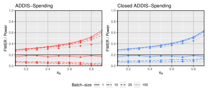
In this section, we aim to quantify the gain in power when using closed ADDIS-Spending instead of ADDIS-Spending and show its FWER control by means of simulations. For this purpose, we first describe the simulation design and then show the results. We considered similar simulation scenarios as in [36], but generated locally dependent -values instead of independent -values.
5.1 Simulation design
We simulated trials where null hypotheses are tested sequentially. We assume that the local dependence structure of the -values is given by finite batches , , with a fixed batch-size . That means we have batches , and so forth, and the -values within one batch depend on each other while -values from different batches are independent. For this simulation, we considered .
Let , where for , and where is the -dimensional normal distribution, and with and for all and . For each , we test the null hypothesis , where , , with probability and , , otherwise. The -values are calculated by , where is the cumulative distribution function (CDF) of a standard normal distribution. Thus, for a -value of a true hypothesis , , and :
If , we have uniformly distributed null -values which means that for all and while a null -value , , is said to be conservative, if for some [38]. Since is increasing in , the null -values are conservative if and only if and the conservativeness grows with decreasing . The parameters and can be interpreted as proportion of false hypotheses and strength of the alternative, respectively.
For each considered scenario, we simulated independent trials and estimated the power and FWER using closed ADDIS-Spending and ADDIS-Spending.
5.2 Comparison of closed ADDIS-Spending and ADDIS-Spending through simulations
We compared the results when using closed ADDIS-Spending and ADDIS-Spending with respect to FWER and power for different batch-sizes and proportions of false null hypotheses. The FWER is represented by the lines below the global significance level and the power by the lines above it. Thereby, the power is defined as the expected number of rejected hypotheses among all false hypotheses. Both procedures are applied with the parameters , and for all . We do not claim that this choice leads to the highest possible power, but it works well to show the differences between the presented procedures.
The results with uniformly distributed null -values and can be found in Figure 4. As discussed before, closed ADDIS-Spending and ADDIS-Spending coincide under independence of the -values (), by this, the solid lines are identical. However, when some of the -values become dependent (), the power and FWER decrease drastically using ADDIS-Spending, while closed ADDIS-Spending decelerates this decrease such that a higher power is obtained. In addition, we see that closed ADDIS-Spending exhausts the FWER more. Simulations for other parameter choices of , and can be found in the Appendix. In all cases, no differences in the behaviour of closed ADDIS-Spending and ADDIS-Spending are observed compared to those shown in Figure 4.
6 Application on real data
In this section, we apply the presented procedures to real data. First, we consider the IMPC dataset, which aims to identify the influence on the phenotype of each protein-coding mouse gene [23] and which is a standard dataset used in the online multiple testing literature [27, 36]. Second, we apply the procedures on the RECOVERY platform trial [32]. Here, several treatments for severe COVID-19 diseases are tested against a standard of care. The two datasets have significant differences. The IMPC data includes several thousand experiments, while the RECOVERY trial has only tested 12 treatments to date. It is important to note that we are not attempting to draw any conclusions from these datasets; they are merely being used for illustrative purposes.
6.1 IMPC data
The International Mouse Phenotyping Consortium (IMPC) is coordinating a large-scale study to determine the function of all protein-coding mouse genes. To this end, each gene is systematically knocked out and the effect on the phenotype is explored. As the dataset grows over time due to the testing of additional genes, the use of online multiple testing procedures is appropriate [27, 36]. Our evaluation is based on the dataset in the Zenodo repository https://zenodo.org/record/2396572 [29]. The contained -values resulted from the analysis in [18] and follow a batch dependence structure since the same group of mice was used for testing several consecutive hypotheses [36]. In our evaluation, we restrict to of these -values that are arranged in batches.
We compare the number of rejections obtained by Alpha-Spending, closed Alpha-Spending, Online-Graph, ADDIS-Spending and closed ADDIS-Spending at the FWER level . We choose such that for all and , where . Note that the larger the , the faster converges to . As done in [36], we set and for the ADDIS procedures. In addition, we choose for the Online-Graph.
The results are summarized in Table 1. As expected, the Alpha-Spending leads to the least rejections. Closed Alpha-Spending and Online-Graph performed similarly. However, Online-Graph led to more rejections when decreased faster (), while closed Alpha-Spending was superior in case of a slowly decreasing (). Both procedures were outperformed by ADDIS-Spending, which was further improved by closed ADDIS-Spending.
| Procedure | Number of rejections | ||
|---|---|---|---|
| Alpha-Spending | |||
| Closed Alpha-Spending | |||
| Online-Graph | |||
| ADDIS-Spending | |||
| Closed ADDIS-Spending | |||
6.2 RECOVERY platform trial
In a platform trial, several treatment arms are compared to the same control group. In contrast to multi-arm trials, the treatment arms do not enter or leave the trial at the same time and the total number of treatments under evaluation is not pre-defined, leading to an online testing problem [26]. Usually, concurrent control data is used, meaning that a treatment arm is only compared to control patients that were randomised while the treatment arm was in the platform. This leads to a local dependence structure of the -values, since treatment arms that overlap share some control data for testing and those that do not overlap can be considered as independent.
In this section, we compare the rejections achieved by the considered methods when applied to a real ongoing platform trial. The Randomised Evaluation of COVID-19 Therapy (RECOVERY) trial has already tested twelve treatments for severe COVID-19 diseases against a standard of care, while another one is currently recruiting [32]. All -values are available at the website https://www.recoverytrial.net/. The overlapping structure is illustrated in a publication by the data monitoring committee [32].
We apply the same procedures as in Section 6.1. However, since the required evidence in such clinical trials is usually higher, we set . In addition, we choose , , for . This change is because harmonic sequences tend to decrease very fast at the beginning of the sequence. This is negligible if the is rather low, as in Section 6.1. However, in this example, we would choose larger as the number of hypotheses is much lower. This is why we expect a geometric sequence to perform better in low-scale settings. Note that in this case, decreases faster for lower .
We compare the number of rejections and the current individual significance level that would be used to test the next treatment, which is already in the trial but has not yet finished recruitment (see Table 2). The behavior of the procedures looks similar as in Section 6.1. However, while the number of rejections does not differ much, closed ADDIS-Spending tests the current hypothesis at the highest level such that the differences between the number of rejections will possibly be larger when further hypotheses are tested. As noted in Section 4.2, closed Alpha-Spending and Online-Graph coincide when is proportional to a geometric sequence and .
| Procedure | Number of rejections | |||||
|---|---|---|---|---|---|---|
| Alpha-Spending | ||||||
| Closed Alpha-Spending | ||||||
| Online-Graph | ||||||
| ADDIS-Spending | ||||||
| Closed ADDIS-Spending | ||||||
7 Discussion
Contemporary problems, e.g. platform trials and genetics research studies, require control of the FWER in unbounded and sequential multiple testing settings [26]. Since the closure principle is fundamental for the construction of multiple testing procedures with FWER control, an extension of the theory is essential. We introduced a novel online closure principle, including a predictability condition for the family of online intersection tests which ensures that the resulting closed testing procedure can be applied in the online setting. Important properties that hold in the classical multiple testing case were transferred to the class of online closed procedures. It was shown that all online procedures with FWER control are also online closed procedures. With this, one can focus on the construction of online closed procedures when aiming for FWER control. Moreover, we proved that one can restrict to consonant families of intersection tests and provided a sufficient condition under which the event of rejecting any hypothesis cannot be enlarged. In addition, we showed how short-cuts of online closed procedures can be obtained under consonance. These have a simpler form than in classical multiple testing as the rejection of an intersection hypothesis uniquely determines which individual hypothesis is to be rejected. We used this to derive individual significance levels for short-cuts that are based on -adjustments. With that, new online closed procedures can be derived easily that often improve existing ones which we have demonstrated with the examples of Alpha-Spending and ADDIS-Spending.
In this paper we focused on the construction of FWER controlling procedures. In online multiple testing, however, many applications aim for a less conservative error rate, e.g. FDR. The reason for this can also be seen when we look at the online procedures that were considered in this paper (e.g. Definition 4.5 and 4.11). Except for unrealistic extreme cases, the individual significance levels of all these procedures will tend to for to infinity. That is because every additional test increases the probability of committing at least one type I error and thus increases the FWER, whereas rejections may lead to a decrease of the FDR. One could say that both types of procedures have an overall level available at the beginning of the testing process. But while FWER controlling procedures can only to spend the level on testing, FDR controlling procedures also allow to gain additional significance level from rejections [8]. Nevertheless, in practice an online multiple testing problem does not necessarily mean that thousands or even millions of hypotheses will be tested, but rather that the number and concrete structure of hypotheses that will be tested is unknown. For example, in platform trials, there may be only a low number of hypotheses to be tested. But since new treatments will be tested over time, online control of the FWER might be required [26]. In another approach, that was especially constructed for the modification of machine learning algorithms, the considered online error rate is only controlled over some time window [6]. In this way, significance level is gained back when hypotheses leave the window, which also makes it reasonable to consider conservative error measures, such as the FWER, in the online setting. A similar approach was considered in [24], where the past is ignored in a smooth manner.
Furthermore, there are approaches to use the closure principle to control other error rates than FWER, such as false discovery proportion (FDP) tail probabilities [13]. Various types of error rates fall under FDP, such as k-FWER and false discovery exceedance (FDX), and it can even be shown that any admissible FDP procedure must also be a closed procedure [11]. In the Appendix, we show that our approach can trivially be extended to obtain an online closure principle for FDP control. However, it is unclear whether the admissibility results derived in [11] and the short-cuts derived in [12] still apply in this case. This could be addressed in future work.
There also exist connections between FDR and closed testing. In [28], they introduced an approach to use graphical procedures for FDR control and, in [12], a connection between Simes-based closed testing and the Benjamini-Hochberg procedure [1] was shown. In addition, every FDR controlling procedure provides weak FWER control and thereby defines an -level intersection test. Hence, all procedures that were constructed for FDR control can be used to derive new closed testing procedures with FWER or FDP control. This is especially interesting in the online case, as the literature is more advanced for FDR control than for FWER and FDP control.
Appendix
Online closure principle for FDP control
The false discovery proportion (FDP) for a some , where we denote by the set of all finite subsets of , is defined as
Note that we focus on finite . On the one hand, is not well-defined for infinite . On the other hand, from a practical point of view, in most applications we will not have an infinite number of hypotheses at hand, as the infinite testing process is only assumed because we do not know how many hypotheses are to be tested in the future. Therefore, we will only be interested in for finite . Following the notation in [11], we are searching for some random function such that for all :
Providing an upper bound for is equivalent to providing a lower bound for the number of true discoveries [11]. Since the number of true discoveries is easier to handle, we are focusing on it in the following. A procedure with true discovery guarantee is a random function such that for all :
Furthermore, we call online true discovery procedure, if is measurable with respect to for all . Thus, the idea is that must be fixed as soon as we can decide on all the individual hypotheses with . The following Theorem is based on the results in [10, 13, 11].
Theorem 7.1 (Online closure principle for true discovery control).
Let a family of -level intersection tests be given. Then the closed procedure , where for all , has true discovery guarantee at level . In addition, if each is an online intersection test and the family of online intersection tests is predictable (Definition 3.1), then is an online procedure.
Proof.
Let be arbitrary. For showing true discovery control of note that implies that for all with . Since , we especially have . However, this happens with probability at most . Thus, . Furthermore, analogously to Lemma 3.3, we can show that due to the predictability of , it holds . Since all are online intersection tests, is measurable with respect to . ∎
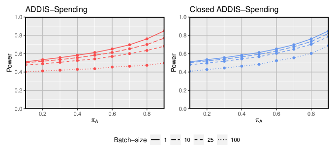
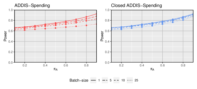
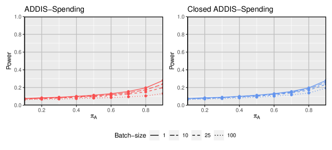
Additional simulation results
In this section we provide additional simulation results based on the design described in Section 5.1. We applied closed ADDIS-Spending and ADDIS-Spending with the same parameters as in Section 5.2. Figure 5 shows the results for conservative -values (). In Figure 6 and Figure 7, we reduced the number of hypothesis to and the strength of the alternative to , respectively, and in Figure 8 we reduced these parameters simultaneously. When we considered the lower number of hypotheses, we also reduced the batch-sizes to . All plots show the similar behavior that closed ADDIS-Spending is less sensitive than ADDIS-Spending to an increase of the batch-size and thus to locally dependent -values.

Omitted proofs
Proof of Theorem 3.9.
We show by induction that for all .
Initial Case (): The predictability of and Lemma 3.3 immediately implies that if and only if .
Induction Hypothesis (IH): We assume that for all , where is arbitrary but fixed.
Induction Step (): “” Since , immediately implies . “” Assume and consider an arbitrary subset with . The consonance property implies that there exists a such that for all with . Since for all and for all , the index satisfying the consonance property has to be . Thus, can be rejected by if . If , the definition of ensures that there exists a with such that . The induction hypothesis then implies that is rejected by and hence is rejected by . Since was arbitrary, all with and can be rejected. Moreover, Lemma 3.3 implies that is rejected by . ∎
Lemma 7.2.
Proof.
“” Assume . Then there exists a such that . Since , the predictability of ensures that and hence . Because for all , we have , meaning . “” implies by definition. ∎
Acknowledgments
The authors are grateful for the valuable comments of two anonymous referees and an associate editor, which have led to significant improvements of the paper. In addition, the authors would like to thank Jelle Goeman for a useful discussion.
Funding
L. Fischer acknowledges funding by the Deutsche Forschungsgemeinschaft (DFG, German Research Foundation) – Project number 281474342/GRK2224/2.
M. Bofill Roig is a member of the EU Patient-centric clinical trial platform (EU-PEARL). EU-PEARL has received funding from the Innovative Medicines Initiative 2 Joint Undertaking under grant agreement No 853966. This Joint Undertaking receives support from the European Union’s Horizon 2020 research and innovation programme and EFPIA and Children’s Tumor Foundation, Global Alliance for TB Drug Development non-profit organization, Spring- works Therapeutics Inc. This publication reflects the author’s views. Neither IMI nor the European Union, EFPIA, or any Associated Partners are responsible for any use that may be made of the information contained herein.
Supplementary Material
The code for the simulations can be found at the GitHub repository https://github.com/fischer23/Closed-Online-Procedures.
References
- Benjamini and Hochberg, [1995] Benjamini, Y. and Hochberg, Y. (1995). Controlling the false discovery rate: A practical and powerful approach to multiple testing. Journal of the Royal Statistical Society: Series B (Statistical Methodology), 57(1):289–300.
- Bittman et al., [2009] Bittman, R. M., Romano, J. P., Vallarino, C., and Wolf, M. (2009). Optimal testing of multiple hypotheses with common effect direction. Biometrika, 96(2):399–410.
- Bretz et al., [2009] Bretz, F., Maurer, W., Brannath, W., and Posch, M. (2009). A graphical approach to sequentially rejective multiple test procedures. Statistics in Medicine, 28(4):586–604.
- Dmitrienko et al., [2003] Dmitrienko, A., Offen, W. W., and Westfall, P. H. (2003). Gatekeeping strategies for clinical trials that do not require all primary effects to be significant. Statistics in Medicine, 22(15):2387–2400.
- Döhler et al., [2021] Döhler, S., Meah, I., and Roquain, E. (2021). Online multiple testing with super-uniformity reward. arXiv preprint arXiv:2110.01255.
- Feng et al., [2021] Feng, J., Emerson, S., and Simon, N. (2021). Approval policies for modifications to machine learning-based software as a medical device: A study of bio-creep. Biometrics, 77(1):31–44.
- Feng et al., [2022] Feng, J., Pennllo, G., Petrick, N., Sahiner, B., Pirracchio, R., and Gossmann, A. (2022). Sequential algorithmic modification with test data reuse. In Uncertainty in Artificial Intelligence, pages 674–684. PMLR.
- Foster and Stine, [2008] Foster, D. P. and Stine, R. A. (2008). -investing: A procedure for sequential control of expected false discoveries. Journal of the Royal Statistical Society: Series B (Statistical Methodology), 70(2):429–444.
- Gabriel, [1969] Gabriel, K. R. (1969). Simultaneous test procedures–some theory of multiple comparisons. The Annals of Mathematical Statistics, 40(1):224–250.
- Genovese and Wasserman, [2006] Genovese, C. R. and Wasserman, L. (2006). Exceedance control of the false discovery proportion. Journal of the American Statistical Association, 101(476):1408–1417.
- Goeman et al., [2021] Goeman, J. J., Hemerik, J., and Solari, A. (2021). Only closed testing procedures are admissible for controlling false discovery proportions. The Annals of Statistics, 49(2):1218–1238.
- Goeman et al., [2019] Goeman, J. J., Meijer, R. J., Krebs, T. J., and Solari, A. (2019). Simultaneous control of all false discovery proportions in large-scale multiple hypothesis testing. Biometrika, 106(4):841–856.
- Goeman and Solari, [2011] Goeman, J. J. and Solari, A. (2011). Multiple testing for exploratory research. Statistical Science, 26(4):584–597.
- Grechanovsky and Hochberg, [1999] Grechanovsky, E. and Hochberg, Y. (1999). Closed procedures are better and often admit a shortcut. Journal of Statistical Planning and Inference, 76(1-2):79–91.
- Hommel et al., [2007] Hommel, G., Bretz, F., and Maurer, W. (2007). Powerful short-cuts for multiple testing procedures with special reference to gatekeeping strategies. Statistics in Medicine, 26(22):4063–4073.
- Ioannidis, [2005] Ioannidis, J. P. (2005). Why most published research findings are false. PLoS medicine, 2(8):e124.
- Javanmard and Montanari, [2018] Javanmard, A. and Montanari, A. (2018). Online rules for control of false discovery rate and false discovery exceedance. The Annals of statistics, 46(2):526–554.
- Karp et al., [2017] Karp, N. A., Mason, J., Beaudet, A. L., Benjamini, Y., Bower, L., Braun, R. E., Brown, S. D., Chesler, E. J., Dickinson, M. E., Flenniken, A. M., et al. (2017). Prevalence of sexual dimorphism in mammalian phenotypic traits. Nature Communications, 8(1):1–12.
- Kohavi et al., [2013] Kohavi, R., Deng, A., Frasca, B., Walker, T., Xu, Y., and Pohlmann, N. (2013). Online controlled experiments at large scale. In Proceedings of the 19th ACM SIGKDD international conference on Knowledge discovery and data mining, pages 1168–1176.
- Lehmann et al., [1986] Lehmann, E. L., Romano, J. P., and Casella, G. (1986). Testing statistical hypotheses, volume 3. Springer.
- Marcus et al., [1976] Marcus, R., Peritz, E., and Gabriel, K. R. (1976). On closed testing procedures with special reference to ordered analysis of variance. Biometrika, 63(3):655–660.
- Maurer et al., [1995] Maurer, W., Hothorn, L., and Lehrmacher, W. (1995). Multiple comparisons in drug clinical trials and preclinical assays: a-priori ordered hypotheses. In Joachim, V., editor, Biometrie in der Chemisch-Pharmazeutischen Industrie, pages 3–18. Fischer Verlag, Stuttgart.
- Muñoz-Fuentes et al., [2018] Muñoz-Fuentes, V., Cacheiro, P., Meehan, T. F., Aguilar-Pimentel, J. A., Brown, S. D., Flenniken, A. M., Flicek, P., Galli, A., Mashhadi, H. H., Hrabě de Angelis, M., et al. (2018). The international mouse phenotyping consortium (impc): A functional catalogue of the mammalian genome that informs conservation. Conservation Genetics, 19(4):995–1005.
- Ramdas et al., [2017] Ramdas, A., Yang, F., Wainwright, M. J., and Jordan, M. I. (2017). Online control of the false discovery rate with decaying memory. Advances in Neural Information Processing Systems, 30.
- Ramdas et al., [2018] Ramdas, A., Zrnic, T., Wainwright, M., and Jordan, M. (2018). Saffron: An adaptive algorithm for online control of the false discovery rate. In International Conference on Machine Learning, pages 4286–4294. PMLR.
- [26] Robertson, D. S., Wason, J., König, F., Posch, M., and Jaki, T. (2022a). Online error control for platform trials. arXiv preprint arXiv:2202.03838.
- [27] Robertson, D. S., Wason, J., and Ramdas, A. (2022b). Online multiple hypothesis testing for reproducible research. arXiv preprint arXiv:2208.11418.
- Robertson et al., [2020] Robertson, D. S., Wason, J. M., and Bretz, F. (2020). Graphical approaches for the control of generalized error rates. Statistics in Medicine, 39(23):3135–3155.
- Robertson et al., [2019] Robertson, D. S., Wildenhain, J., Javanmard, A., and Karp, N. A. (2019). onlinefdr: An r package to control the false discovery rate for growing data repositories. Bioinformatics, 35(20):4196–4199.
- Romano et al., [2011] Romano, J. P., Shaikh, A., and Wolf, M. (2011). Consonance and the closure method in multiple testing. The International Journal of Biostatistics, 7(1):0000102202155746791300.
- Romano and Wolf, [2005] Romano, J. P. and Wolf, M. (2005). Exact and approximate stepdown methods for multiple hypothesis testing. Journal of the American Statistical Association, 100(469):94–108.
- Sandercock et al., [2022] Sandercock, P. A., Darbyshire, J., DeMets, D., Fowler, R., Lalloo, D. G., Munavvar, M., Staplin, N., Warris, A., Wittes, J., and Emberson, J. R. (2022). Experiences of the data monitoring committee for the RECOVERY trial, a large-scale adaptive platform randomised trial of treatments for patients hospitalised with COVID-19. Trials, 23(1):881.
- Schweder and Spjøtvoll, [1982] Schweder, T. and Spjøtvoll, E. (1982). Plots of p-values to evaluate many tests simultaneously. Biometrika, 69(3):493–502.
- Sonnemann and Finner, [1988] Sonnemann, E. and Finner, H. (1988). Vollständigkeitssätze für multiple testprobleme. In Bauer, P., Hommel, G., and Sonnemann, E., editors, Multiple Hypothesenprüfung/Multiple Hypotheses Testing, pages 121–135. Springer, Berlin.
- Tian and Ramdas, [2019] Tian, J. and Ramdas, A. (2019). Addis: An adaptive discarding algorithm for online fdr control with conservative nulls. Advances in Neural Information Processing Systems, 32.
- Tian and Ramdas, [2021] Tian, J. and Ramdas, A. (2021). Online control of the familywise error rate. Statistical Methods in Medical Research, 30(4):976–993.
- Zehetmayer et al., [0] Zehetmayer, S., Posch, M., and Koenig, F. (0). Online control of the false discovery rate in group-sequential platform trials. Statistical Methods in Medical Research, 0(0):09622802221129051. PMID: 36189481.
- Zhao et al., [2019] Zhao, Q., Small, D. S., and Su, W. (2019). Multiple testing when many p-values are uniformly conservative, with application to testing qualitative interaction in educational interventions. Journal of the American Statistical Association, 114(527):1291–1304.
- Zrnic et al., [2020] Zrnic, T., Jiang, D., Ramdas, A., and Jordan, M. (2020). The power of batching in multiple hypothesis testing. In International Conference on Artificial Intelligence and Statistics, pages 3806–3815. PMLR.
- Zrnic et al., [2021] Zrnic, T., Ramdas, A., and Jordan, M. I. (2021). Asynchronous online testing of multiple hypotheses. J. Mach. Learn. Res., 22:33–1.