A Curriculum-Training-Based Strategy for Distributing Collocation Points during Physics-Informed Neural Network Training

Abstract

Physics-informed Neural Networks (PINNs) often have, in their loss functions, terms based on physical equations and derivatives. In order to evaluate these terms, the output solution is sampled using a distribution of collocation points. However, density-based strategies, in which the number of collocation points over the domain increases throughout the training period, do not scale well to multiple spatial dimensions. To remedy this issue, we present here a curriculum-training-based method for lightweight collocation point distributions during network training. We apply this method to a PINN which recovers a full two-dimensional magnetohydrodynamic (MHD) solution from a partial sample taken from a baseline MHD simulation. We find that the curriculum collocation point strategy leads to a significant decrease in training time and simultaneously enhances the quality of the reconstructed solution.

1 Introduction

Solving partial differential equations (PDEs) is a fundamental task in space physics. Although numerical algorithms have tremendously improved over the years [Weinan et al., (2021)], providing solutions over a full space-time domain often requires large-scale, computationally-intensive simulations. As an alternative to such simulations, machine learning (ML) techniques have become popular in recent years, fusing physics and data (e.g., soft proton predictions [Kronberg et al., (2021)], solar flare forecasts [Nishizuka et al., (2021)], or space weather forecasts [Camporeale, (2019)]). However, most of these approaches rely on huge datasets which appropriately cover the relevant domain. This approach cannot work for domains with a sparsity problem, e.g., spacecraft missions in planetary magnetospheres in which the amount of data recorded is very tiny compared to the amount of data inherent in the global system.

One way to address this sparsity problem is to numerically solve the physical equations over the full domain given specific initial and boundary conditions. However, such global simulations can be quite costly, requiring many thousands of computer core hours. Additionally, they are not yet sophisticated enough to assimilate data and modify their solutions appropriately to match observations. As an alternative, PINNs can alleviate the sparsity problem by combining data observations and physical constraints in their loss functions to reconstruct global contexts around local data samples (e.g. the one-dimensional magnetohydrodynamics reconstructions in [Bard and Dorelli, (2021)]). This has the potential to provide a lightweight alternative to global simulations, but only if the PINN is able to train quickly.

In order to generate physically-valid solutions, PINNs ensure that their output solutions correctly correspond to their inherent physical equations [Raissi et al., (2019); Karniadakis et al., (2021)]. These calculations require so-called "collocation points" distributed through the domain at which the solution and its derivatives are evaluated and tested against the physical equations. The simplest strategy for distributing collocation points is to randomly scatter them throughout the domain and increase the density of points as network training progresses. Other strategies include evolutionary sampling, which gradationally aggregates points in areas of high PDE loss residuals [Daw et al., (2022)], or the importance method, which samples collocation points according to a distribution proportional to the loss function [Nabian et al., (2021)]. Currently, one of the major obstacles in developing a PINN-based solver for three-dimensional reconstruction of space plasmas is the poor scaling to multiple dimensions. The previously mentioned density-based strategy requires increasingly significant computational resources as the dimensionality goes up [Bard and Dorelli, (2021)]. In this paper, we present two novel curriculum-training-based approaches using lightweight collocation point distributions that better scale to multiple dimensions. We apply these methods to a PINN which recovers a full two-dimensional MHD solution from a partial sample of simulated spacecraft observations. We find that the new strategy leads to a significant decrease in training time and simultaneously enhances the quality of the reconstructed solution.

2 Model Setup

We use a PINN designed to reconstruct two-dimensional MHD solutions given partial linear samples of the original solution, mimicking the reconstruction of space environments from satellite data. This extends the one-dimensional network of [Bard and Dorelli, (2021)] to two dimensions. The rebuild of higher-dimensional plasma space-time is interpreted as a regression problem of form

$$\mathbf{U}^{st}\approx f([\mathbf{x};\mathbf{y};\mathbf{t}]\mid\mathbf{\theta})\coloneqq\mathbf{U}_{net}(x,y,t)$$ (1)

where $\mathbf{U}^{st}$ is the full MHD solution, $\mathbf{x}$ and $\mathbf{y}$ are the spatial positions, and $\mathbf{t}$ is time. $[~{};~{}]$ denotes concatenation and $\theta$ are model parameters that are to be found through training. The approximated solution $\mathbf{U}_{net}$ follows both a physical constraint

$$\frac{\partial\mathbf{U}_{net}}{\partial t}+F(\mathbf{U}_{net},\frac{\partial\mathbf{U}_{net}}{\partial x})+G(\mathbf{U}_{net},\frac{\partial\mathbf{U}_{net}}{\partial y})=0$$ (2)

and a boundary data constraint

$$\mathbf{U}_{net}(x_{i},y_{i},t_{i})=\mathbf{U}^{st}_{i},\;i=1\dots N_{d}$$ (3)

for $N_{d}$ coordinates of $(x,y,t)$ in space-time. $F$ and $G$ are the two-dimensional MHD fluxes (see Appendix A.2 for further details).

In order to mimic satellite observations in space, every experiment builds on four randomly chosen linear trajectories that are constrained to cover the full time range but only a small part of the spatial domain. We emulate sparse craft measurements by sampling a portion of approximately $10^{-6}$ points per trajectory in comparison to the full space-time grid. As recent PINNs primarily incorporate dense neural networks [Chiu et al., (2022), e.g. Hennigh et al., (2020)], we implement our PINN as a Multi-Layer Perceptron Regressor [Rosenblatt, (1958); Mcculloch and Pitts, (1943)]. Its weights are trained by the ADAM optimizer [Kingma and Ba, (2014)] while respecting a predefined learning rate schedule [You et al., (2019)] to improve the convergence curve of the model [Bard and Dorelli, (2021)]. Hyperparameters are tuned using the Tree-structured Parzen Estimator Approach [Bergstra et al., (2011)] and trials get pruned by applying median pruning. We enforce five startup runs during which the pruning is disabled.

The loss function is defined as $L_{PINN}=(L_{data}+\lambda L_{phys})/(1+\lambda)$ where $L_{data},L_{phys}$ represent the data and physical loss, and $\lambda$ is a trade-off parameter balancing these two. The physical loss is evaluated at collocation points distributed within the reconstruction domain. Previous work reconstructing plasma solutions around spacecraft trajectories [Bard and Dorelli, (2021)] used density-based collocation point sampling in which the density of collocation points in space-time increases over the training interval. However, this does not scale well to higher spatial dimensions; in fact, the density-based run time can be expressed as $\mathcal{O}(n_{T}+n_{C}^{d+1})$ [Mala and Ali, (2022)], where $n_{T}$ is the number of data points and $n_{C}$ is the number of collocation points required to satisfy a specific collocation density in each of the $d$ spatial dimensions and one time dimension. Increasing the density has a larger effect on runtime with increasing dimensionality.

Hence, the collocation point sampling method needs to be independent of the problem dimensionality for the PINN to scale well. Thus, we define the set of sampled collocation points per epoch as a constant matching the number of spacecraft observations, which results in a linear runtime of $\mathcal{O}(n_{T}+n_{C})\cong\mathcal{O}(n_{T})$. This provides a significant speedup in comparison to density-based collocation point sampling, but we must be intentional in how we distribute the points.

3 Curriculum Strategies

The beginnings of curriculum learning in the field of ML can at least be backtraced to [Elman, (1993)]. Inspired by human education, it is based on the idea of guiding a learning process by increasing the difficulty level of tasks over time [Bengio et al., (2009); Soviany et al., (2021)]. Originally, this is done by feeding a model easy-to-learn data first, and then gradually transitioning to more complex data concepts [Bengio et al., (2009)]. Curriculum training has already demonstrated its potential to improve various machine learning models for different applications, for instance MLPs for healthcare prediction [El-Bouri et al., (2020)], CNNs for computer vision [Jafarpour et al., (2021)], RNNs for language modeling [Shi et al., (2014)], and even PINNs for solving one-dimensional MHD problems [Krishnapriyan et al., (2021)]. Here, we propose two novel curriculum strategies for our PINN training.

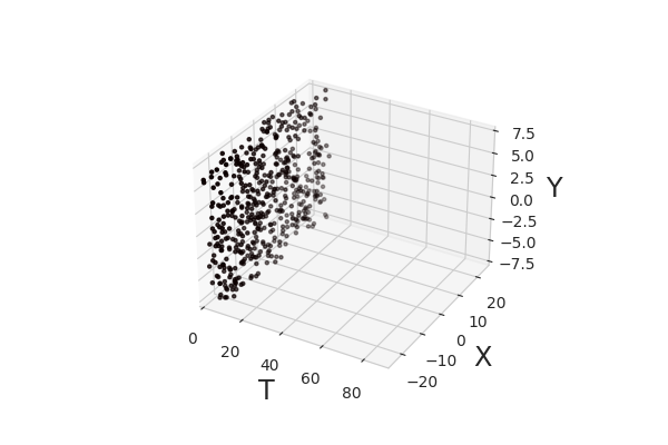
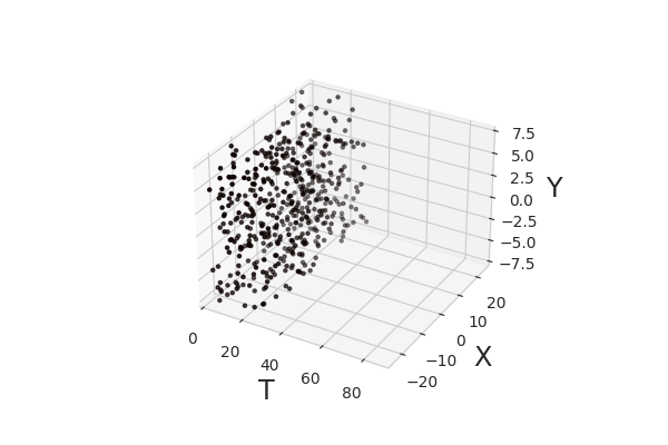
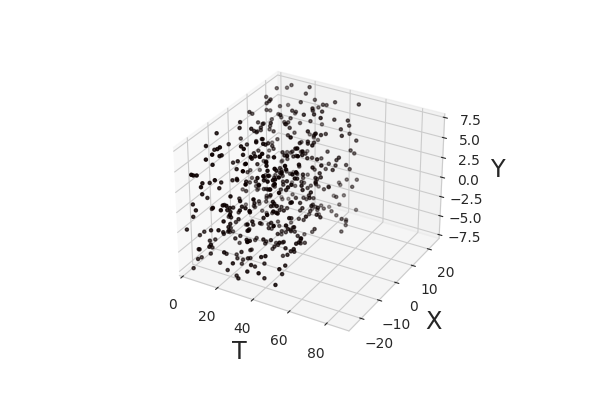
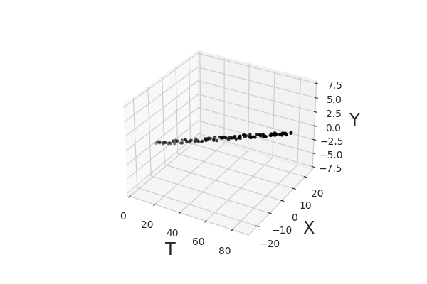
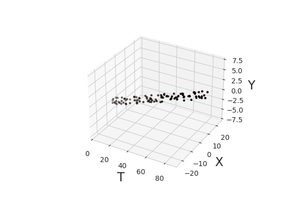
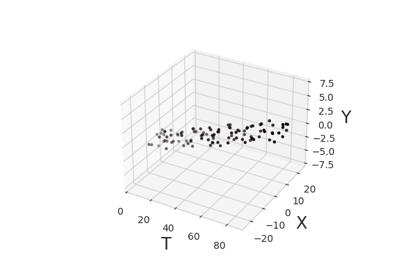
(a) Cuboid sampling step 0 (b) Cuboid sampling step 1 (c) Cuboid sampling step 2 (d) Cylinder sampling step 0 (e) Cylinder sampling step 1 (f) Cylinder sampling step 2

Figure 1: Evolution of collocation point distributions for the Cuboid and Cylinder Curriculum methods over several training epochs.

First, we define a sampling method whereby the initial collocation point distribution is a cuboid covering the full space domain but only in a very small time range starting at $t_{0}$. As training progresses, the cuboid gradually extends along the time axis, eventually encompassing the full reconstruction domain. In this way, the model first builds up an accurate reconstruction of the time-dependent behavior at initial times and then expands this knowledge throughout the training (an example is shown in Figure 1). Analogously, the model could also be supported in its training by stretching out the cuboid to the full (x, t) domain and extending along y, or to the full (y, t) domain and extending along x. This is referred to as the cuboid curriculum method.

Alternatively, we hypothesize that regions closer to the sparse training data points are easier to reconstruct than ones further away in space-time. To take advantage of this, we distribute collocation points in small-radius spheres around the labeled training data and then stepwise increase the radii of these bubbles until they cover the whole space-time domain. For our specific use-case here (Sec. 2), the data points are arranged linearly in space; consequently, the collocation points are located in a cylinder with increasing radius (e.g. Figure 1) around the linear spacecraft trajectories. This strategy is referred to as the cylinder curriculum method, though it can be generalized to a bubble method.

4 Results

We test the curriculum training methods on three different datasets. First, an MHD reconnection benchmark from [Birn et al., (2001)] (name: GEM) of the following resolution: $-25.60\leq x<25.60$ with $\Delta x=0.04$, $-7.68\leq y<7.68$ with $\Delta y=0.04$, and $0\leq t\leq 90$ with $\Delta t=0.45$; resulting in a mesh of $1280\times 384\times 201$ (correspondingly $98,795,520\approx 10^{8}$ points in total). Second, we use a 2D Riemann Problem based on Case 3 from [Liska and Wendroff, (2003)] (name: LW3). Since this is technically a hydrodynamic benchmark, we artificially inflate its plasma state vectors by adding the magnetic variables $B$ and setting them to zero. We run the base simulation until $t=0.35$ with an output every $\Delta t=5\times 10^{-3}$. The spatial dimensions are resolved as $0\leq x<1$ with $\Delta x\approx 5\times 10^{-4}$, and $0\leq y<1$ with $\Delta y\approx 5\times 10^{-4}$; leading to a grid of $2048\times 2048\times 71$ and a total of $297,795,584\approx 3\times 10^{9}$ voxels. Finally, we explore an MHD vortex [Orszag and Tang, (1979)] designed to study turbulence (name: OT). It is represented as a mesh of $1024\times 1024\times 50$ (consequently $98,795,520\approx 10^{8}$ overall points) where $0\leq x<1$ with $\Delta x\approx 10^{-2}$, $0\leq y<1$ with $\Delta y\approx 10^{-3}$, and $0\leq t<1$ with $\Delta t=0.02$.

Figure 2: PINN convergence epoch for the GEM data (left axes), the LW3 data (center axes), and the OT test data (right axes).

In addition to the cuboid and cylinder curriculum methods, we test a baseline strategy of randomly distributing the collocation points throughout the full space-time domain, also resampling them every epoch. We train the models for a maximum of 5,000 epochs, with the curriculum training covering the initial $30\%$ (1500 epochs) of the training period. We extend the collocation point distribution five (15) times for the cuboid (cylinder) method, or every 300 (100) epochs until full coverage. This was experimentally chosen to ensure high accuracy. 50 experiments were run for each dataset and curriculum method. Each trial took about six minutes on an Nvidia Tesla V100 GPU at the Compute Cloud of the Leibniz Supercomputing Centre (45 computing hours total).

Figures 2 and 3 show the mean squared error and the training speed as measured by the average number of epochs to convergence. We find that the curriculum-trained networks converged faster and to a lower error than the random-collocation-trained network. On average, the curriculum networks took $\approx 35\%$ fewer epochs to converge, though the cuboid+GEM model took approximately the same amount of epochs as the random+GEM model. Thus, the cylinder (or bubble) method performed slightly better overall than the cuboid method, albeit this depends on the scenario. Finally, the reconstruction accuracy increased: the cuboid and cylinder curriculum methods achieved an improvement of up to $\approx 72\%$, and $\approx 32\%$ on average.

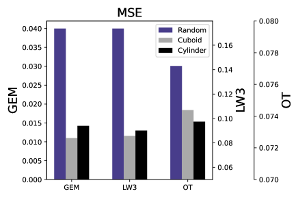
Figure 3: PINN mean squared error for the GEM data (left axes; purple), the LW3 data (center axes), and the OT test data (right axes).

5 Discussion and Conclusion

We find that the curriculum training method for distributing collocation points significantly enhances PINN MHD reconstructions, simultaneously boosting accuracy and reducing time to convergence. However, we note that our results depend on the scenario and the models’ initializations. Although the experiments here are robust, it is not guaranteed that our findings are universally applicable to every plasma environment. We note that hyperparameters, including the number of collocation points and the rate of expansion for the distribution, greatly influence the results. Future work may look for heuristics to fully exploit these strategies, possibly taking advantage of local loss errors [Nabian et al., (2021)]. Alternatively, the methods can be applied to 3D simulations. We envision an even more powerful runtime supremacy here, though this remains to be tested.

Appendix A Appendix

A.1 Reproducing Experiments

The experiments are based on the code of [Münzer, (2022)].
We use the following datasets: GEM [Münzer and Bard, 2022a ], LW3 [Münzer and Bard, 2022b ], and OT [Münzer and Bard, 2022c ].

A.2 MHD Equations

The three-dimensional magnetohydrodynamic equations (using primitive variables) are:

$$\frac{\partial\rho}{\partial t}+\nabla\cdot(\rho\vec{v})=0$$ (4)

$$\rho\frac{\partial\vec{v}}{\partial t}+\rho\vec{v}\cdot\nabla\vec{v}=-\nabla P+(\nabla\times\vec{B})\times\vec{B}+{\color[rgb]{1,0,0}\rho\nu\nabla^{2}\vec{v}}$$ (5)

$$\frac{\partial P}{\partial t}+\vec{v}\cdot\nabla P+\gamma P\nabla\cdot\vec{v}=0$$ (6)

$$\frac{\partial\vec{B}}{\partial t}=\nabla\times\left(\vec{v}\times\vec{B}\right)+{\color[rgb]{1,0,0}\eta\nabla^{2}\vec{B}}$$ (7)

$$\nabla\cdot\vec{B}=0$$ (8)

We note that the ideal MHD equations do not contain the terms in red, which are the effects of viscosity ($\nu\nabla^{2}\vec{v}$) and resistivity ($\eta\nabla^{2}\vec{B}$). The simulations used to generate the test problems in this paper (LW3, GEM, OT) did not include these terms. However, based on results from [Michoski et al., (2020)] and [Bard and Dorelli, (2021)], we add these terms to the PINN loss function in order to smooth out and better reconstruct the final solution near discontinuities (e.g., shock fronts). We clarify that the PINN cannot reproduce a discontinuous solution; however, adding viscosity and resistivity terms helps reproduce a steep, smooth solution where there is a discontinuity in the original simulation.

For the 2D PINN used in this paper, we convert these equations to two spatial dimensions by assuming $\partial/\partial z=\partial^{2}/\partial z^{2}=0$. The full set of equations, expanded out to individual derivatives, is:

$$\frac{\partial\rho}{\partial t}+\frac{\partial(\rho v_{x})}{\partial x}+\frac{\partial(\rho v_{y})}{\partial y}=0$$

$$\rho\frac{\partial v_{x}}{\partial t}+\rho v_{x}\frac{\partial v_{x}}{\partial x}+\rho v_{y}\frac{\partial v_{x}}{\partial y}+\frac{\partial P}{\partial x}+B_{z}\frac{\partial B_{z}}{\partial x}+B_{y}\left(\frac{\partial B_{y}}{\partial x}-\frac{\partial B_{x}}{\partial y}\right)-\rho\nu\left(\frac{\partial^{2}v_{x}}{\partial x^{2}}+\frac{\partial^{2}v_{x}}{\partial y^{2}}\right)=0$$

$$\rho\frac{\partial v_{y}}{\partial t}+\rho v_{x}\frac{\partial v_{y}}{\partial x}+\rho v_{y}\frac{\partial v_{y}}{\partial y}+\frac{\partial P}{\partial y}-B_{x}\left(\frac{\partial B_{y}}{\partial x}-\frac{\partial B_{x}}{\partial y}\right)+B_{z}\frac{\partial B_{z}}{\partial y}-\rho\nu\left(\frac{\partial^{2}v_{y}}{\partial x^{2}}+\frac{\partial^{2}v_{y}}{\partial y^{2}}\right)=0$$

$$\rho\frac{\partial v_{z}}{\partial t}+\rho v_{x}\frac{\partial v_{z}}{\partial x}+\rho v_{y}\frac{\partial v_{z}}{\partial y}-B_{y}\frac{\partial B_{z}}{\partial y}-B_{x}\frac{\partial B_{z}}{\partial x}-\rho\nu\left(\frac{\partial^{2}v_{z}}{\partial x^{2}}+\frac{\partial^{2}v_{z}}{\partial y^{2}}\right)=0$$

$$\frac{\partial P}{\partial t}+v_{x}\frac{\partial P}{\partial x}+v_{y}\frac{\partial P}{\partial y}+\gamma P\left(\frac{\partial v_{x}}{\partial x}+\frac{\partial v_{y}}{\partial y}\right)=0$$

$$\frac{\partial B_{x}}{\partial t}-\frac{\partial}{\partial y}\left(v_{x}B_{y}-v_{y}B_{x}\right)-\eta\left(\frac{\partial^{2}B_{x}}{\partial x^{2}}+\frac{\partial^{2}B_{x}}{\partial y^{2}}\right)=0$$

$$\frac{\partial B_{y}}{\partial t}+\frac{\partial}{\partial x}\left(v_{x}B_{y}-v_{y}B_{x}\right)-\eta\left(\frac{\partial^{2}B_{y}}{\partial x^{2}}+\frac{\partial^{2}B_{y}}{\partial y^{2}}\right)=0$$

$$\frac{\partial B_{z}}{\partial t}-\frac{\partial}{\partial x}\left(v_{z}B_{x}-v_{x}B_{z}\right)+\frac{\partial}{\partial y}\left(v_{y}B_{z}-v_{z}B_{y}\right)-\eta\left(\frac{\partial^{2}B_{z}}{\partial x^{2}}+\frac{\partial^{2}B_{z}}{\partial y^{2}}\right)=0$$

$$\frac{\partial B_{x}}{\partial x}+\frac{\partial B_{y}}{\partial y}=0$$

The values for $\nu$ and $\eta$ are set by hyperparameter optimization with respect to the overall training loss. The final values suggested by the optimization are: $\nu=1.24*10^{-4}$ and $\eta=1.88*10^{-3}$ (GEM); $\nu=1.58*10^{-3}$ and $\eta=6.87*10^{-3}$ (LW3); $\nu=2.76*10^{-3}$ and $\eta=5.59*10^{-3}$ (OT). We note that [Bard and Dorelli, (2021)] tested the effect of changing $\nu$ on the reconstructed solution for a 1D MHD shock tube; that study found that the best value for $\nu$ depends on the problem. This motivated us to use hyperparameter optimization for choosing appropriate values.

References

- Bard and Dorelli, (2021) Bard, C. and Dorelli, J. (2021). Neural network reconstruction of plasma space-time. Frontiers in Astronomy and Space Sciences, 8:146–160.
- Bengio et al., (2009) Bengio, Y., Louradour, J., Collobert, R., and Weston, J. (2009). Curriculum learning. In Proceedings of the 26th Annual International Conference on Machine Learning, ICML ’09, page 41–48, New York, NY, USA. Association for Computing Machinery.
- Bergstra et al., (2011) Bergstra, J., Bardenet, R., Bengio, Y., and Kégl, B. (2011). Algorithms for hyper-parameter optimization. In Shawe-Taylor, J., Zemel, R., Bartlett, P., Pereira, F., and Weinberger, K. Q., editors, Advances in Neural Information Processing Systems, volume 24. Curran Associates, Inc.
- Birn et al., (2001) Birn, J., Drake, J. F., Shay, M. A., Rogers, B. N., Denton, R. E., Hesse, M., Kuznetsova, M., Ma, Z. W., Bhattacharjee, A., Otto, A., and Pritchett, P. L. (2001). Geospace environmental modeling (gem) magnetic reconnection challenge. jgr, 106(A3):3715–3720.
- Camporeale, (2019) Camporeale, E. (2019). The challenge of machine learning in space weather nowcasting and forecasting.
- Chiu et al., (2022) Chiu, P.-H., Wong, J. C., Ooi, C., Dao, M. H., and Ong, Y.-S. (2022). CAN-PINN: A fast physics-informed neural network based on coupled-automatic–numerical differentiation method. Computer Methods in Applied Mechanics and Engineering, 395:114909.
- Daw et al., (2022) Daw, A., Bu, J., Wang, S., Perdikaris, P., and Karpatne, A. (2022). Rethinking the importance of sampling in physics-informed neural networks.
- El-Bouri et al., (2020) El-Bouri, R., Eyre, D., Watkinson, P., Zhu, T., and Clifton, D. (2020). Student-teacher curriculum learning via reinforcement learning: Predicting hospital inpatient admission location.
- Elman, (1993) Elman, J. L. (1993). Learning and development in neural networks: the importance of starting small. Cognition, 48(1):71–99.
- Hennigh et al., (2020) Hennigh, O., Narasimhan, S., Nabian, M. A., Subramaniam, A., Tangsali, K., Rietmann, M., Ferrandis, J. d. A., Byeon, W., Fang, Z., and Choudhry, S. (2020). Nvidia simnet tm: an ai-accelerated multi-physics simulation framework.
- Jafarpour et al., (2021) Jafarpour, B., Pogrebnyakov, N., and Sepehr, D. (2021). Active curriculum learning. In InterNLP 2021. First Workshop on Interactive Learning for Natural Language Processing, pages 40–45, United States. Association for Computational Linguistics. First Workshop on Interactive Learning for Natural Language Processing. InterNLP 2021 ; Conference date: 05-08-2021 Through 05-08-2021.
- Karniadakis et al., (2021) Karniadakis, G. E., Kevrekidis, I. G., Lu, L., Perdikaris, P., Wang, S., and Yang, L. (2021). Physics-informed machine learning. Nature Reviews Physics, 3(6).
- Kingma and Ba, (2014) Kingma, D. P. and Ba, J. (2014). Adam: A method for stochastic optimization.
- Krishnapriyan et al., (2021) Krishnapriyan, A., Gholami, A., Zhe, S., Kirby, R., and Mahoney, M. (2021). Characterizing possible failure modes in physics-informed neural networks.
- Kronberg et al., (2021) Kronberg, E. A., Hannan, T., Huthmacher, J., Münzer, M., Peste, F., Zhou, Z., Berrendorf, M., Faerman, E., Gastaldello, F., Ghizzardi, S., Escoubet, P., Haaland, S., Smirnov, A., Sivadas, N., Allen, R. C., Tiengo, A., and Ilie, R. (2021). Prediction of soft proton intensities in the near-earth space using machine learning. The Astrophysical Journal, 921(1):76.
- Liska and Wendroff, (2003) Liska, R. and Wendroff, B. (2003). Comparison of several difference schemes on 1d and 2d test problems for the euler equations. SIAM Journal on Scientific Computing, 25(3):995–1017.
- Mala and Ali, (2022) Mala, F. and Ali, R. (2022). The big-o of mathematics and computer science. 6:1–3.
- Mcculloch and Pitts, (1943) Mcculloch, W. and Pitts, W. (1943). A logical calculus of ideas immanent in nervous activity. Bulletin of Mathematical Biophysics, 5:127–147.
- Michoski et al., (2020) Michoski, C., Milosavljevic, M., Oliver, T., and Hatch, D. (2020). Solving differential equations using deep neural networks. Neurocomputing, 399.
- Münzer, (2022) Münzer, M. (2022). marcus-muenzer/Neural-Network-Reconstruction-of- higher-dimensional-Plasma-Space-Time: Release Version V1.0 (github, zenodo).
- (21) Münzer, M. and Bard, C. (2022a). Gem plasma space-time (zenodo).
- (22) Münzer, M. and Bard, C. (2022b). Lw3 plasma space-time (zenodo).
- (23) Münzer, M. and Bard, C. (2022c). Ot plasma space-time (zenodo).
- Nabian et al., (2021) Nabian, M. A., Gladstone, R. J., and Meidani, H. (2021). Efficient training of physics-informed neural networks via importance sampling. Computer-Aided Civil and Infrastructure Engineering, 36(8):962–977.
- Nishizuka et al., (2021) Nishizuka, N., Kubo, Y., Sugiura, K., Den, M., and Ishii, M. (2021). Operational solar flare prediction model using deep flare net.
- Orszag and Tang, (1979) Orszag, S. A. and Tang, C. M. (1979). Small-scale structure of two-dimensional magnetohydrodynamic turbulence. Journal of Fluid Mechanics, 90:129–143.
- Raissi et al., (2019) Raissi, M., Perdikaris, P., and Karniadakis, G. (2019). Physics-informed neural networks: A deep learning framework for solving forward and inverse problems involving nonlinear partial differential equations. Journal of Computational Physics, 378:686–707.
- Rosenblatt, (1958) Rosenblatt, F. (1958). The perceptron: a probabilistic model for information storage and organization in the brain. Psychological review, 65(6):386.
- Shi et al., (2014) Shi, Y., Larson, M., and Jonker, C. (2014). Recurrent neural network language model adaptation with curriculum learning. Computer Speech and Language, 33.
- Soviany et al., (2021) Soviany, P., Ionescu, R. T., Rota, P., and Sebe, N. (2021). Curriculum learning: A survey.
- Weinan et al., (2021) Weinan, E., Jiequn, H., and Arnulf, J. (2021). Algorithms for solving high dimensional PDEs: from nonlinear monte carlo to machine learning. Nonlinearity, 35(1):278–310.
- You et al., (2019) You, K., Long, M., Wang, J., and Jordan, M. I. (2019). How does learning rate decay help modern neural networks?