Precise Asymptotics for Spectral Methods
in Mixed Generalized Linear Models

Abstract

In a mixed generalized linear model, the objective is to learn multiple signals from unlabeled observations: each sample comes from exactly one signal, but it is not known which one. We consider the prototypical problem of estimating two statistically independent signals in a mixed generalized linear model with Gaussian covariates. Spectral methods are a popular class of estimators which output the top two eigenvectors of a suitable data-dependent matrix. However, despite the wide applicability, their design is still obtained via heuristic considerations, and the number of samples $n$ needed to guarantee recovery is super-linear in the signal dimension $d$. In this paper, we develop exact asymptotics on spectral methods in the challenging proportional regime in which $n,d$ grow large and their ratio converges to a finite constant. By doing so, we are able to optimize the design of the spectral method, and combine it with a simple linear estimator, in order to minimize the estimation error. Our characterization exploits a mix of tools from random matrices, free probability and the theory of approximate message passing algorithms. Numerical simulations for mixed linear regression and phase retrieval display the advantage enabled by our analysis over existing designs of spectral methods.

1 Introduction

We consider the problem of learning multiple $d$-dimensional vectors from $n$ unlabeled observations coming from a mixed generalized linear model (GLM):

$$y_{i} =q\left(\left\langle a_{i},x_{\eta_{i}}^{*}\right\rangle,\varepsilon_{i}\right),\qquad i\in[n]=\{1,\ldots,n\}.$$ (1.1)

Here, $x_{1}^{*},\ldots,x_{\ell}^{*}\in\mathbb{R}^{d}$ are the $\ell$ signals (regression vectors) to be recovered from the observation vector $y=(y_{1},\ldots,y_{n})\in\mathbb{R}^{n}$ and the known design matrix $A=[a_{1},\ldots,a_{n}]^{\top}\in\mathbb{R}^{n\times d}$. For $i\in[n]$, $\varepsilon_{i}$ is a noise variable, and $\eta_{i}$ is an $[\ell]$-valued latent variable, i.e., it indicates which signal each observation comes from, and is unknown to the statistician. The notation $\left\langle\cdot,\cdot\right\rangle$ denotes the Euclidean inner product, and $q:\mathbb{R}^{2}\to\mathbb{R}$ is a known link function. For $\ell=1$, Equation 1.1 reduces to a generalized linear model [MN89], which covers many widely studied problems in statistical estimation including linear regression, logistic regression, phase retrieval [SEC⁺15, FS20], and 1-bit compressed sensing [BB08]. The regression model with $\ell=1$ implicitly assumes a homogeneous population, in which a single regression vector suffices to capture the features of the entire sample. In practice, it is often the case that the observations may come from multiple sub-populations. Mixed GLMs offer a flexible solution in settings with unlabeled heterogeneous data, and have found applications in a variety of fields including biology, physics, and economics [MP04, GL07, LSL19, DGP20]. When $q(g,\varepsilon)=g+\varepsilon$, Equation 1.1 reduces to the widely studied mixture of linear regressions [VT02, FS10, SBvdG10, CL13, YCS14, ZJD16, SS19, ZMCL20, GK20].

A natural approach to estimate the vectors $x_{1}^{*},\ldots,x_{\ell}^{*}$ from $y$ and $A$ is via the maximum-likelihood estimator (assuming a statistical model for $(\varepsilon_{i})_{i\in[n]}$ is available). However, the corresponding optimization problem is non-convex and NP-hard [YCS14]. Thus, various low-complexity alternatives — mostly focusing on mixed linear regression — have been proposed: examples include expectation-maximization (EM) [KC07, FS10, SBvdG10], alternating minimization [YCS14, SS19, GK20], convex relaxation [CYC14], moment descent methods [LL18, CLS20], and the use of tractable non-convex objectives [ZJD16, BH22]. Many of these methods are iterative in nature and require a “warm start” with an initial guess correlated with the ground truth. Spectral methods represent a popular way to provide such initialization [YCS14]. A variety of estimators based on the spectral decomposition of data-dependent matrices or tensors has been proposed for mixed GLMs [CL13, YCS14, SJA16]. In this paper, we focus on a spectral method that estimates the $\ell$ signals via the top-$\ell$ principal eigenvectors of the following data-dependent matrix:

$$D=\frac{1}{n}\sum_{i=1}^{n}{\mathcal{T}}(y_{i})a_{i}a_{i}^{\top}\in{\mathbb{R}}^{d\times d},$$ (1.2)

where $\mathcal{T}:\mathbb{R}\to\mathbb{R}$ is a suitably chosen preprocessing function. This spectral estimator with the preprocessing function ${\mathcal{T}}(y)=y^{2}$ was studied for mixed linear regression by Yi et al. [YCS14], who showed that the signals can be accurately recovered when the number of observations $n$ is of order $d\log d$. Furthermore, existing theoretical results for all estimators (including spectral, alternating minimization and EM) require the number of observations $n$ to be of order at least $d\log d$ to guarantee accurate recovery [CL13, YCS14, SJA16, LL18, CLS20]. This leads to the following natural questions:

What is the optimal sample complexity of a spectral estimator based on Equation 1.2?
Can we carry out a principled optimization of the preprocessing function ${\mathcal{T}}$?

A simpler alternative to obtain an initial estimate is to employ the linear estimator

$$\frac{1}{n}\sum_{i=1}^{n}{\mathcal{L}}(y_{i})a_{i}\ \in{\mathbb{R}}^{d},$$ (1.3)

where ${\mathcal{L}}:{\mathbb{R}}\to{\mathbb{R}}$ is a suitable preprocessing function. The performance analysis of this linear estimator for the mixed GLM can be carried out similarly to that for the non-mixed case ($\ell=1$); the analysis for the latter is given in [PVY17, Proposition 1] and in [MTV21, Lemma 2.1]. Thus, a second natural question is:

What is the optimal way to combine a spectral estimator based on Equation 1.2 and the linear estimator in Equation 1.3?

1.1 Main contributions

In this paper, we resolve the questions above for the prototypical setting of the recovery of two independent signals $x_{1}^{*},x_{2}^{*}$ with a Gaussian design matrix $A$. This is achieved by characterizing the high-dimensional limit of the joint empirical distribution of (i) the signals $x_{1}^{*},x_{2}^{*}$, (ii) the linear estimator in Equation 1.3, and (iii) spectral estimators based on the matrix in Equation 1.2. Our analysis holds in the proportional setting where $n,d\to\infty$ with $n/d\to\delta\in(0,\infty)$. That is, we consider the regime where the ratio between sample size and signal dimension tends to a constant, as opposed to most analyses of mixed GLMs in the literature which assume $n=\Omega(d\log d)$. Our major findings are summarized as follows.

• Our master theorem (Theorem 3.1) characterizes the joint distribution of the linear estimator, the spectral estimator, and the signals in the high-dimensional limit. This joint distribution characterization holds for arbitrary preprocessing functions ${\mathcal{L}},{\mathcal{T}}\colon{\mathbb{R}}\to{\mathbb{R}}$ in Equations 1.2 and 1.3 (subject to certain mild regularity conditions). The limiting joint distribution is expressed as the law of a set of jointly Gaussian random variables whose covariance structure is explicitly derived in terms of the model and the preprocessing functions.

• As an immediate consequence of the above characterization, we derive the normalized correlations (or ‘overlaps’) between the linear/spectral estimator and the signals (Corollary 3.3/Corollary 3.5). The linear estimator achieves a strictly positive overlap with each signal for any $\delta>0$, provided a strictly positive overlap can be attained for some $\delta>0$. In contrast, for the spectral estimator, we identify a threshold (depending on the preprocessing function ${\mathcal{T}}$) such that strictly positive overlap is attained as soon as $\delta$ exceeds this threshold.

• Our master theorem also allows us to compute the limiting overlap of a class of combinations of linear and spectral estimators. In particular, the Bayes-optimal combination can be derived, which turns out to be a linear combination of the two estimators due to the Gaussianity of their high-dimensional limits (Corollary 3.2).

• We determine the optimal preprocessing functions ${\mathcal{L}}^{*},{\mathcal{T}}_{1}^{*},{\mathcal{T}}_{2}^{*}\colon{\mathbb{R}}\to{\mathbb{R}}$ for the linear and spectral estimators that maximize the overlap between the estimator and each signal (Proposition 3.4 and Proposition 3.6). The optimal overlaps of linear and spectral estimators reveal intriguing behaviors of mixed models. In particular, there is a single function ${\mathcal{L}}^{*}$ that simultaneously maximizes the overlap between the linear estimator and each signal. In contrast, for the spectral method, one needs to employ two different functions ${\mathcal{T}}_{1}^{*},{\mathcal{T}}_{2}^{*}$ in order to achieve the maximal overlaps with $x_{1}^{*}$, $x_{2}^{*}$, respectively. Furthermore, the optimal overlap of the spectral estimator with each signal approaches $1$ — the best possible value — as the aspect ratio $\delta$ grows. We remark that the same is not true for the linear estimator: the optimal overlap with each signal remains strictly less than 1 even as $\delta\to\infty$, as long as there is a strictly positive fraction of observations corresponding to each signal.

• Finally, we specialize our results to two canonical settings: mixed linear regression (Corollaries 3.7 and 3.8) and mixed phase retrieval (Corollary 3.9). In the noiseless case, even though the two models are distinct, spectral estimators have the same performance on both. In contrast, the linear estimator exhibits non-trivial performance for linear regression, whereas it always results in vanishing overlap for phase retrieval.

Our precise asymptotic analysis leads to a significant improvement over previous designs of spectral methods, as showcased in Figure 1 for noiseless mixed linear regression. The continuous lines correspond to our theoretical predictions (“pred.”), which closely match the points coming from the simulations (“sim.”). The following methods are compared: (i) optimal spectral method (black), obtained from Proposition 3.6; (ii) optimal linear method (blue), obtained from Proposition 3.4; (iii) combined estimator (“combo”) (red), obtained from Corollary 3.2; (iv) spectral estimator for mixed linear regression proposed in [YCS14] (yellow); (v) spectral estimator which optimizes the overlap in the non-mixed setting (green), proposed in [LAL19]. The spectral methods resulting from our sharp analysis (red, black) significantly outperform existing methods (green, yellow), especially for low values of $\delta$. More details on the experimental setup and additional simulation results can be found in Section 4.

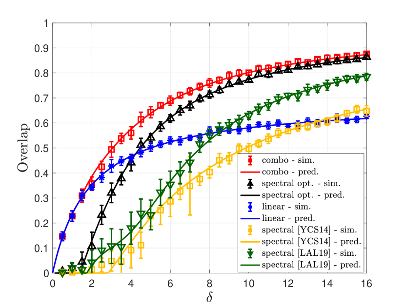
(a) Recovery of $x_{1}^{*}$

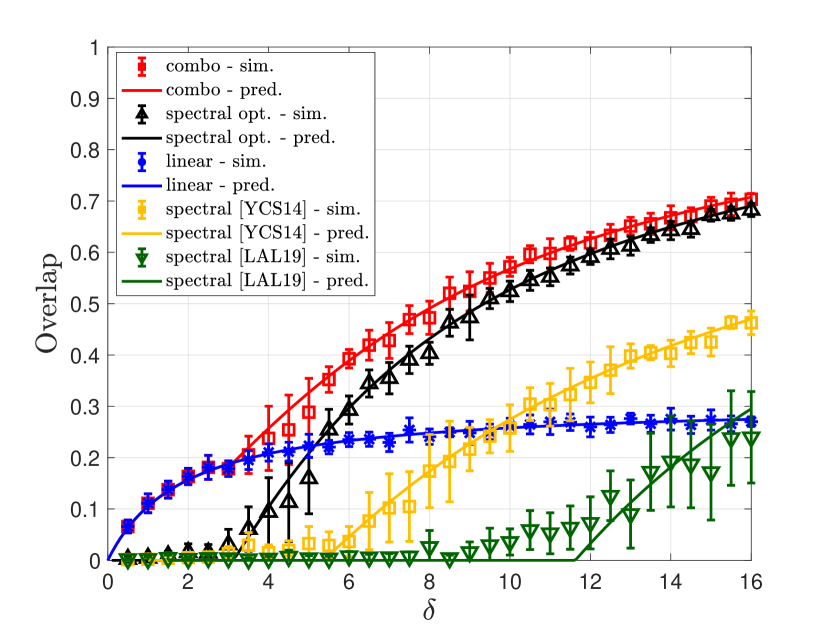
(b) Recovery of $x_{2}^{*}$

Figure 1: Noiseless mixed linear regression with mixing parameter (i.e., probability that a sample corresponds to $x_{1}^{*}$) $\alpha=0.6$. Overlaps with the first signal $x_{1}^{*}$ (left) and the second signal $x_{2}^{*}$ (right), computed via simulation (“sim.”) and the theoretical prediction (“pred.”), are plotted as a function of the aspect ratio $\delta=n/d$. The signal dimension is $d=2000$.

Proof techniques.

We exploit a combination of tools from free probability, random matrices and the theory of approximate message passing. More specifically, generalized approximate message passing (GAMP) refers to a family of iterative algorithms [Ran11] with the following key feature: the joint distribution of the iterates is accurately tracked by a simple deterministic recursion, called state evolution. Our strategy to obtain the joint distribution of the linear/spectral estimators and the signals in the master theorem (Theorem 3.1) is to design a GAMP that (i) outputs the linear estimator as the first iterate and (ii) then implements a power method, so that its fixed point corresponds to the spectral estimator. One challenge in the implementation of this strategy is that the state evolution of GAMP, in its original form for vanilla (non-mixed) GLMs, only records the correlation of its iterates with a single signal. To circumvent this issue, we equip GAMP with a state evolution recursion involving both signals, and run a pair of GAMP iterations converging to the first and second top eigenvector of the spectral matrix in Equation 1.2, respectively. A second – even more fundamental – challenge is that, for the power method to converge to the desired eigenvector, a spectral gap between the corresponding eigenvalue and the rest of the spectrum is required. For non-mixed GLMs, the spectral analysis was carried out in earlier work [LL20, MM19], and both eigenvalues and overlaps were characterized using tools from random matrix theory. Here, the difficulty comes from the mixed effect of the model, leading to additional matrix terms which appear to be difficult to control. Our approach is to decompose $D$ into the sum of two matrices, $D_{1}$ and $D_{2}$, each consisting of components only pertaining to the first and second signal, respectively. Now, $D_{1},D_{2}$ can be individually viewed as generated from a non-mixed GLM, hence their limiting spectra are well understood. The key observation is then that, by assuming both signals to be independent and uniformly distributed on the sphere, $D_{1}$ and $D_{2}$ become asymptotically free. Thus, we are able to characterize the sum of these two spiked matrices by using techniques from free probability.

1.2 Related work

We review below the three lines of literature most closely related to our work, which concern mixtures of generalized linear models, spectral methods and the theory of approximate message passing algorithms.

Mixtures of generalized linear models.

Mixtures of generalized linear models have been studied in machine learning under the name ‘hierarchical mixtures of experts’, see e.g., [JJ94]. Bayesian methods for inference in this model were investigated in [PJT96] and [WMR95], and Bayesian inference for the special case of mixed linear regression (MLR) was analyzed in [VT02].

Khalili and Chen [KC07] proposed a penalized likelihood approach for variable selection in mixed GLMs, and showed consistency of the procedure in the low-dimensional setting (where the dimension $d$ is fixed as $n$ grows). Städler et al. [SBvdG10] analyzed $\ell_{1}$-penalized estimators for high-dimensional mixed linear regression. Recently Zhang et al. [ZMCL20] studied estimation and inference for high-dimensional mixed linear regression with two sparse components, in the setting where the mixing proportion and the covariance structure of the covariates are unknown. The works [KC07, SBvdG10, ZMCL20] all use variants of the EM algorithm for optimizing a suitable penalized likelihood function.

Balakrishnan et al. [BWY17] and Klusowski et al. [KYB19] obtained statistical guarantees on the performance of the EM algorithm for a class of problems, including the special case of symmetric mixed linear regression (MLR) where $x_{1}^{*}=-x_{2}^{*}$. Variants of the EM algorithm for symmetric MLR in the high-dimensional setting (with sparse signals) were analyzed in [WGNL15, YC15, ZWZG17]. Minimax lower bounds for a class of computationally feasible algorithms for symmetric MLR were obtained in [FLWY18]. Kong et al. [KSS⁺20] studied MLR as a canonical example of meta-learning: in the setting where the number of signals ($\ell$) is large, they derived conditions under which a large number of signals with a few observations can compensate for the lack of signals with abundantly many observations. The prediction error of MLR in the non-realizable setting, where no generative model is assumed for the data, was studied in [PMSG22]. Chandrasekher et al. [CPT21] recently analyzed the performance of a class of iterative algorithms (not including AMP) for mixtures of GLMs. They provide a sharp characterization of the per-iteration error with sample-splitting in the regime $n\asymp d\,\mathrm{polylog}(d)$, assuming a Gaussian design and a random initialization.

Spectral methods.

We first review spectral methods based on Equation 1.2 for standard GLMs (non-mixed, with $\ell=1$), which were introduced in [Li92]. For the special case of phase retrieval, a series of works has provided increasingly refined bounds on the number of samples needed to guarantee signal recovery via the spectral method [NJS13, CSV13, CC15]. This type of analysis is based on matrix concentration inequalities, a technique that typically does not return exact values for the overlap between the signal and the estimate. More recently, an exact high-dimensional analysis for generalized linear models was carried out in [LL20, MM19]. These works focus on the regime of interest in this paper: $n$ and $d$ growing at a proportional rate $\delta\coloneqq\lim\frac{n}{d}$. This sharp analysis allows for the optimization of the preprocessing function: the choice of ${\mathcal{T}}$ minimizing the value of $\delta$ (and, hence, the amount of data) needed to achieve a strictly positive overlap was provided in [MM19]; furthermore, the choice of ${\mathcal{T}}$ maximizing the overlap was provided in [LAL19]. The analysis of the spectral methods in the works above assumes a Gaussian design matrix. Going beyond this assumption, [DBMM20] provides precise asymptotics for design matrices sampled from the Haar distribution, and [MKLZ22] studies rotationally invariant designs.

Moving to the mixed regression setting ($\ell>1$), Yi et al. [YCS14] proposed a spectral estimator based on Equation 1.2 with ${\mathcal{T}}(y)=y^{2}$. The analysis is based on concentration inequalities and requires the number of samples $n$ to be of order $d\log d$ for accurate recovery. Estimators based on spectral decomposition of data-dependent tensors were proposed for MLR in [CL13] and for mixed GLMs in [SJA16]. However, these methods require $n$ to be of order at least $d^{3}$ for accurate recovery. Our work is the first to establish exact asymptotics for a mixed GLM in the linear sample-size regime: $n,d\to\infty$ with $n/d\to\delta\in(0,\infty)$. To achieve this goal, our strategy differs from analyses of spectral methods in the non-mixed setting [LL20, MM19] which reduces the study of the spectrum of $D$ to that of a rank-1 perturbation. In contrast, our analysis is based on a combination of techniques from free probability and approximate message passing.

Approximate message passing (AMP) algorithms.

AMP is a family of iterative algorithms that has been applied to several problems in high-dimensional statistics, including estimation in linear models [DMM09, BM11, KMS⁺12], generalized linear models [Ran11, SR14, SC19], and low-rank matrix estimation [DM14, RFG09, LKZ17]. For a broad overview, we refer the reader to [FVRS22]. A key feature of AMP algorithms is that under suitable model assumptions, the empirical joint distribution of their iterates can be exactly characterized in the high-dimensional limit, in terms of a simple scalar recursion called state evolution. By taking advantage of this characterization, AMP methods have been used to derive exact high-dimensional asymptotics for convex penalized estimators such as LASSO [BM12], M-estimators [DM16], logistic regression [SC19], and SLOPE [BKRS20]. AMP algorithms have been initialized via spectral methods in the context of low-rank matrix estimation [MV21c] and generalized linear models [MV21a]. Furthermore, they have been used – in a non-mixed setting – to combine linear and spectral estimators [MTV21]. A finite-sample analysis which allows the number of iterations to grow roughly as $\log n$ ($n$ being the ambient dimension) was put forward in [RV18], and the recent paper [LW22] improves this guarantee to a linear (in $n$) number of iterations. This could potentially allow to study settings in which $\delta=n/d$ approaches the spectral threshold. The works on AMP discussed above all assume i.i.d. Gaussian matrices. A number of recent papers has proposed generalizations of AMP for the much broader class of rotationally invariant matrices, e.g., [OCW16, MP17, RSF19, Tak20, ZSF21, Fan22, MV21b, VKM22].

Organization of the paper.

Formal definitions for the mixed GLM, linear estimators and spectral estimators are presented in Section 2. Our main results are stated in Section 3: these include the master theorem (Theorem 3.1) and its various consequences (whose proofs are deferred to Appendices A, B, C, D and E). Numerical simulations are provided in Section 4. The proof of Theorem 3.1 is divided across two sections. Section 5 contains a characterization of the top three eigenvalues of the matrix $D$ which will be useful in the analysis of GAMP in the following section. The limiting joint law of the signal, the linear and the spectral estimators in Theorem 3.1 is then proved in Section 6 using a GAMP algorithm and its characterization via state evolution. The proof of the state evolution characterization is deferred to Appendix H. The main body of the paper is concluded with discussions in Section 7. Some background on random matrix and free probability theory is provided in Appendices F and G, and several auxiliary lemmas used in our proofs are listed in Appendix I.

2 Preliminaries

2.1 Notation

The $i$-th element in a vector $a\in{\mathbb{R}}^{p}$ is denoted by $a_{i}\in{\mathbb{R}}$. If a vector has multiple subscripts, the component index is always the last one. For a symmetric matrix $M\in{\mathbb{R}}^{p\times p}$, we denote by $\mu_{M}$ the empirical spectral distribution of $M$. The (real) eigenvalues of $M$ are denoted by $\lambda_{1}(M)\geq\lambda_{2}(M)\geq\cdots\geq\lambda_{p}(M)$, and the corresponding eigenvectors of unit norms are denoted by $v_{1}(M),v_{2}(M),\cdots,v_{p}(M)$. The $(i,j)$-th entry of $M$ is denoted by $M_{i,j}$. For a random variable $X$, we use $\operatorname{supp}(X)$ to denote the support of its density function. For a set ${\mathcal{S}}\subset{\mathbb{R}}$ of real numbers, denote by $\sup({\mathcal{S}})\coloneqq\sup\{x:x\in{\mathcal{S}}\}$ its least upper bound. The orthogonal group in dimension $p$ is denoted by ${\mathbb{O}}(p)\coloneqq\left\{O\in{\mathbb{R}}^{p\times p}:OO^{\top}=O^{\top}O=I_{p}\right\}$. The unit sphere in dimension $p$ is denoted by ${\mathbb{S}}^{p-1}\coloneqq\left\{x\in{\mathbb{R}}^{p}:\left\|x\right\|_{2}=1\right\}$. For two distributions $P$ and $Q$, we use $P\otimes Q$ to denote the product distribution with $P$ (resp. $Q$) being its first (resp. second) marginal. For an integer $k\geq 2$, $P^{\otimes k}$ denotes the $k$-fold product distribution of $P$.

2.2 Model

We consider a two-component mixed generalized linear model (mixed GLM) with signal vectors $x_{1}^{*},x_{2}^{*}\in{\mathbb{S}}^{d-1}$, covariate vectors $a_{1},\cdots,a_{n}\in{\mathbb{R}}^{d}$ , and a known link function $q\colon{\mathbb{R}}^{2}\to{\mathbb{R}}$. Let $P_{\varepsilon}$ be a noise distribution over ${\mathbb{R}}$. The $n$ observations $y_{1},\cdots,y_{n}\in{\mathbb{R}}$ are generated as:

$$y_{i} =q\left(\left\langle a_{i},\eta_{i}x_{1}^{*}+(1-\eta_{i})x_{2}^{*}\right\rangle,\,\varepsilon_{i}\right),\qquad i\in[n].$$ (2.1)

Here, the vector of latent variables ${\underline{\eta}}\coloneqq(\eta_{1},\cdots,\eta_{n})\sim\operatorname{Bern}(\alpha)^{\otimes n}$ indicates which signal is selected by each observation, and is unobserved. The vector ${\underline{\eta}}$ is independent of the signals $x_{1}^{*},x_{2}^{*}$ and the covariate vectors $a_{1},\ldots,a_{n}$. The noise vector ${\underline{\varepsilon}}\coloneqq(\varepsilon_{1},\cdots,\varepsilon_{n})\sim P_{\varepsilon}^{\otimes n}$ is independent of $x_{1}^{*},x_{2}^{*},{\underline{\eta}}$, in which case Equation 2.1 becomes

$$y_{i}\,|\,\left\langle a_{i},\eta_{i}x_{1}^{*}+(1-\eta_{i})x_{2}^{*}\right\rangle\sim p(\cdot\,|\,\left\langle a_{i},\eta_{i}x_{1}^{*}+(1-\eta_{i})x_{2}^{*}\right\rangle),$$ (2.2)

where $p(\cdot|g)$ denotes the distribution of $q(g,\varepsilon)$ for a fixed $g\in\mathbb{R}$ and $\varepsilon\sim P_{\varepsilon}$ independent of $g$. The design matrix $A\in{\mathbb{R}}^{n\times d}$ is formed by collecting all $(a_{i})_{i\in[n]}$ as rows:

$$A \coloneqq\begin{bmatrix}a_{1}^{\top}\\ \vdots\\ a_{n}^{\top}\end{bmatrix}\in{\mathbb{R}}^{n\times d}.$$

Given $A$, upon observing $y=(y_{1},\cdots,y_{n})\in{\mathbb{R}}^{n}$, our goal is to estimate $x_{1}^{*}$ and $x_{2}^{*}$. Given a pair of estimators $\widehat{x}_{1}=\widehat{x}_{1}(y,A),\,\widehat{x}_{2}=\widehat{x}_{2}(y,A)\in{\mathbb{R}}^{d}$, a performance measure of central interest is their overlap with the respective signals:

$$\lim_{d\to\infty}\frac{\left|\left\langle\widehat{x}_{1},x_{1}^{*}\right\rangle\right|}{\left\|\widehat{x}_{1}\right\|_{2}\left\|x_{1}^{*}\right\|_{2}},\quad\lim_{d\to\infty}\frac{\left|\left\langle\widehat{x}_{2},x_{2}^{*}\right\rangle\right|}{\left\|\widehat{x}_{2}\right\|_{2}\left\|x_{2}^{*}\right\|_{2}}.$$

Throughout the paper, the following assumptions are imposed.

1. $x_{1}^{*},x_{2}^{*}$ are independent and uniformly distributed on unit sphere, $(x_{1}^{*},x_{2}^{*})\sim\operatorname{Unif}({\mathbb{S}}^{d-1})^{\otimes 2}$.

2. $\alpha\in(1/2,1)$.

3. The noise sequence ${\underline{\varepsilon}}\in{\mathbb{R}}^{n}$ is i.i.d. according to ${\underline{\varepsilon}}\sim P_{\varepsilon}^{\otimes n}$, and $P_{\varepsilon}$ has bounded second moment.

4. $a_{1},\cdots,a_{n}\in{\mathbb{R}}^{d}$ are i.i.d., each distributed according to $a_{i}\overset{\mathrm{i.i.d.}}{\sim}{\mathcal{N}}(0_{d},I_{d})$.

5. We consider the proportional regime where $n,d\to\infty$ and $n/d\to\delta$ for some constant $\delta\geq 0$ which we call aspect ratio.

As for Item (A1), choosing signals uniformly distributed on the sphere corresponds to a setting in which no structural information about them is available (and, therefore, the uniform prior is selected by the statistician). We note that this requirement is natural, since our focus is on spectral methods which are typically unable to exploit prior information about the signal. Understanding the effect of correlation on the design of spectral methods is an exciting avenue for future research.

Item (A2), which implies that a larger fraction of the $n$ observations come from $x_{1}^{*}$ than from $x_{2}^{*}$, is without loss of generality. Otherwise, if $0<\alpha<1/2$, one can simply interchange the roles of $x_{1}^{*}$ and $x_{2}^{*}$. The case $\alpha=1/2$ is special. In this case, as $n\to\infty$, the top two eigenvectors given by the spectral method correspond to the same limiting eigenvalue. These eigenvectors provide an estimate on the space spanned by $x_{1}^{*},x_{2}^{*}$ and, in order to estimate the individual signals, an additional $1$-dimensional grid search has to be performed. Provided this extra step is carried out, our results can be shown to extend to the case $\alpha=1/2$. See Remarks 3.4, 5.2 and 6.2 for more details.

Item (A4) is common in theoretical analyses of spectral estimators for standard (non-mixed) GLMs [YCS14, MM19, LL20, LAL19]. The potential universality of the predictions obtained with Gaussian design matrices is discussed in Section 7.

2.3 Linear estimator

Let ${\mathcal{L}}\colon{\mathbb{R}}\to{\mathbb{R}}$ be a preprocessing function. Then, the linear estimator is defined as

$$\widehat{x}^{\mathrm{lin}} \coloneqq\frac{1}{n}A^{\top}{\mathcal{L}}(y)=\frac{1}{n}\sum_{i=1}^{n}{\mathcal{L}}(y_{i})a_{i}\in{\mathbb{R}}^{d},$$ (2.3)

where ${\mathcal{L}}$ is applied component-wise, i.e., ${\mathcal{L}}(y)=({\mathcal{L}}(y_{1}),\cdots,{\mathcal{L}}(y_{n}))$. Define the random variable $Y$ as

$$Y=q(G,\varepsilon),\quad\text{ where }(G,\varepsilon)\sim{\mathcal{N}}(0,1)\otimes P_{\varepsilon}.$$ (2.4)

We make the following assumption on the preprocessing function ${\mathcal{L}}$ used in the linear estimator.

1. ${\mathcal{L}}\colon{\mathbb{R}}\to{\mathbb{R}}$ is Lipschitz and satisfies the following conditions:

   $$\mathbb{E}\left[G{\mathcal{L}}(Y)\right] \neq 0,\quad\mathbb{E}\left[|G{\mathcal{L}}(Y)|\right]<\infty.$$

As shall be seen in our main result (Theorem 3.1), the first condition in Item (A6) guarantees that the linear method w.r.t. ${\mathcal{L}}$ attains positive overlaps with both signals. The second condition is rather mild and purely technical.

2.4 Spectral estimator

Let ${\mathcal{T}}\colon{\mathbb{R}}\to{\mathbb{R}}$ be a preprocessing function, and consider

$$T \coloneqq\mathrm{diag}({\mathcal{T}}(y))\in{\mathbb{R}}^{n\times n},\quad D\coloneqq\frac{1}{n}A^{\top}TA=\frac{1}{n}\sum_{i=1}^{n}{\mathcal{T}}(y_{i})a_{i}a_{i}^{\top}\in{\mathbb{R}}^{d\times d},$$ (2.5)

where we use again the notation ${\mathcal{T}}(y)=({\mathcal{T}}(y_{1}),\cdots,{\mathcal{T}}(y_{n}))$. Then, the spectral method computes the top two eigenvectors $v_{1}(D),v_{2}(D)$ of $D$ as estimates of $x_{1}^{*},x_{2}^{*}$, respectively. We make the following assumption on the preprocessing function ${\mathcal{T}}$ used in the spectral estimator.

1. ${\mathcal{T}}\colon{\mathbb{R}}\to{\mathbb{R}}$ is Lipschitz and satisfies

   $$\inf_{y\in\operatorname{supp}(Y)}{\mathcal{T}}(y)>-\infty,\quad\text{and}\quad 0<\sup_{y\in\operatorname{supp}(Y)}{\mathcal{T}}(y)<\infty,$$

   where $Y$ is defined in Equation 2.4. We also assume that the random variable ${\mathcal{T}}(Y)$ is not almost surely zero, i.e., $\Pr\left[{\mathcal{T}}(Y)=0\right]<1$.

In words, Item (A7) requires ${\mathcal{T}}$ to be bounded, with the upper edge of its range being strictly positive. Having a bounded preprocessing function is necessary for the spectral method to be effective in the non-mixed setting as well [MM19, LL20]. Furthermore, the requirement on the $\sup$ to be strictly positive is purely technical, and is simply to rule out the trivial cases in which the spectral matrix $D$ is all-zero with high probability. We also note that Item (A7) is satisfied by the preprocessing function that maximizes the overlap (cf. Proposition 3.6).

3 Main results

We start by defining a few auxiliary quantities. Let $\delta_{1}=\alpha\delta,\delta_{2}=(1-\alpha)\delta$, and $Z={\mathcal{T}}(Y)$, with $Y$ as defined in Equation 2.4. Define $\varphi\colon(\sup\operatorname{supp}(Z),\infty)\to{\mathbb{R}}$ and $\psi\colon(\sup\operatorname{supp}(Z),\infty)\times(0,\infty)\to{\mathbb{R}}$ as

$$\varphi(\lambda) \coloneqq\lambda\,\mathbb{E}\left[\frac{ZG^{2}}{\lambda-Z}\right],$$ (3.1)

$$\psi(\lambda;\Delta) \coloneqq\lambda\left(\frac{1}{\Delta}+\mathbb{E}\left[\frac{Z}{\lambda-Z}\right]\right).$$ (3.2)

In what follows, we will set the second argument $\Delta$ of $\psi$ to $\delta,\delta_{1}$ and $\delta_{2}$. For $\Delta\in\{\delta,\delta_{1},\delta_{2}\}$, let $\overline{\lambda}(\Delta)>\sup\operatorname{supp}(Z)$ be the minimum point of $\psi(\cdot;\Delta)$, i.e.,

$$\overline{\lambda}(\Delta) \coloneqq\operatorname*{argmin}_{\lambda>\sup\operatorname{supp}(Z)}\psi(\lambda;\Delta).$$ (3.3)

Since $\psi$ is convex in its first argument (see Lemma I.2), this minimum point is readily obtained by setting the derivative to $0$. Furthermore, define $\zeta\colon(\sup\operatorname{supp}(Z),\infty)\times(0,\infty)\to{\mathbb{R}}$ as

$$\zeta(\lambda;\Delta) \coloneqq\psi(\max\{\lambda,\overline{\lambda}(\Delta)\};\Delta).$$ (3.4)

Finally, for $i\in\{1,2\}$, by [MM19, Lemma 2], we have that the equation $\zeta(\lambda;\delta_{i})=\varphi(\lambda)$ admits a unique solution in $\lambda\in(\sup\operatorname{supp}(Z),\infty)$ which we call $\lambda^{*}(\delta_{i})$. The functions $\psi(\lambda;\Delta),\varphi(\lambda),\zeta(\lambda;\Delta)$ together with the parameters $\lambda^{*}(\Delta),\overline{\lambda}(\Delta)$ are plotted in Figure 2 for $\Delta\in\{\delta,\delta_{1},\delta_{2}\}$. Some convexity and monotonicity properties (which will be useful later in the proofs) of these functions can be found in Lemma I.2.

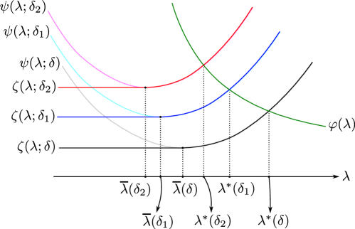
Figure 2: Plot of $\psi(\lambda;\Delta),\varphi(\lambda),\zeta(\lambda;\Delta)$ as functions of $\lambda$ with $\Delta\in\{\delta,\delta_{1},\delta_{2}\}$.

The empirical distribution of a vector $u\in{\mathbb{R}}^{d}$ is given by $\frac{1}{d}\sum_{i=1}^{d}\delta_{u_{i}}$, where $\delta_{u_{i}}$ denotes a Dirac delta mass on $u_{i}$. Similarly, the joint empirical distribution of the rows of a matrix $(u^{1},u^{2},\ldots,u^{t})\in{\mathbb{R}}^{d\times t}$ is $\frac{1}{d}\sum_{i=1}^{d}\delta_{(u^{1}_{i},\ldots,u^{t}_{i})}$. Our master theorem is an exact characterization in the high-dimensional limit of the joint empirical distribution of the rows of the signals, the linear estimator, and the spectral estimators. In particular, we show that this joint empirical distribution converges to the law of a Gaussian random vector with a specified covariance matrix. The result is stated in terms of the following parameters: the asymptotic correlations $\rho_{1}^{\mathrm{lin}},\rho_{2}^{\mathrm{lin}}$ between the linear estimator and the two signals; the normalized length $n^{\mathrm{lin}}$ of the linear estimator; and the asymptotic correlations $\rho_{1}^{\mathrm{spec}},\rho_{2}^{\mathrm{spec}}$ between the spectral estimators and the two signals. The formulas for these quantities are:

$$n^{\mathrm{lin}}\coloneqq\bigg{(}(\alpha^{2}+(1-\alpha)^{2})\mathbb{E}\left[G{\mathcal{L}}(Y)\right]^{2}+\frac{\mathbb{E}\left[{\mathcal{L}}(Y)^{2}\right]}{\delta}\bigg{)}^{\frac{1}{2}},$$ (3.5a)

$$\rho_{1}^{\mathrm{lin}}\coloneqq\frac{\alpha\mathbb{E}\left[G{\mathcal{L}}(Y)\right]}{n^{\mathrm{lin}}},\quad\rho_{2}^{\mathrm{lin}}\coloneqq\frac{(1-\alpha)\mathbb{E}\left[G{\mathcal{L}}(Y)\right]}{n^{\mathrm{lin}}},$$ (3.5b)

$$\rho_{1}^{\mathrm{spec}}\coloneqq\left(\frac{\frac{1}{\delta}-\mathbb{E}\left[\left(\frac{Z}{\lambda^{*}(\delta_{1})-Z}\right)^{2}\right]}{\frac{1}{\delta}+\alpha\mathbb{E}\left[\left(\frac{Z}{\lambda^{*}(\delta_{1})-Z}\right)^{2}(G^{2}-1)\right]}\right)^{\frac{1}{2}},\;\rho_{2}^{\mathrm{spec}}\coloneqq\left(\frac{\frac{1}{\delta}-\mathbb{E}\left[\left(\frac{Z}{\lambda^{*}(\delta_{2})-Z}\right)^{2}\right]}{\frac{1}{\delta}+(1-\alpha)\mathbb{E}\left[\left(\frac{Z}{\lambda^{*}(\delta_{2})-Z}\right)^{2}(G^{2}-1)\right]}\right)^{\frac{1}{2}}.$$ (3.5c)

Theorem 3.1 is stated in terms of pseudo-Lipschitz test functions. A function $\Psi:{\mathbb{R}}^{m}\to{\mathbb{R}}$ is pseudo-Lipschitz of order $k\geq 1$, denoted $\Psi\in{\rm PL}(k)$, if there is a constant $C>0$ such that

$$\left\|\Psi(x)-\Psi(y)\right\|_{2}\leq C(1+\|x\|_{2}^{k-1}+\|y\|_{2}^{k-1})\left\|x-y\right\|_{2},$$ (3.6)

for all $x,y\in\mathbb{R}^{m}$. Examples of pseudo-Lipschitz functions of order two are: $\Psi(u)=u^{2}$ and $\Psi(u,v)=\left|uv\right|$, for $u,v\in{\mathbb{R}}$. For simplicity, we consider pseudo-Lipschitz test functions of order two, as those suffice to compute the asymptotic overlaps between the signals and the various estimators. We note that one could extend Theorem 3.1 to test functions in ${\rm PL}(k)$ for $k>2$, at the cost of a more involved argument and an additional assumption on the boundedness of the moments of $P_{\varepsilon}$.

Theorem 3.1 (Master theorem on joint distribution).

Consider the setting of Section 2, and let Items (A1), (A2), (A3), (A4), (A5), (A6) and (A7) hold. Define the following rescaled vectors of length $\sqrt{d}$: $x^{\mathrm{lin}}=\sqrt{d}\,\widehat{x}^{\mathrm{lin}}/\left\|\widehat{x}^{\mathrm{lin}}\right\|_{2}$, $\overline{x}^{*}_{i}=\sqrt{d}x_{i}^{*}$, $x^{\mathrm{spec}}_{i}=s_{i}\sqrt{d}\,v_{i}(D)$, where the sign $s_{i}\in\{-1,1\}$ is chosen such that $\left\langle s_{i}v_{i}(D),x_{i}^{*}\right\rangle\geq 0$ ($i\in\{1,2\}$). Then, the following holds almost surely for any ${\rm PL}(2)$ function $\Psi:{\mathbb{R}}^{3}\to{\mathbb{R}}$. If $\lambda^{*}(\delta_{1})>\overline{\lambda}(\delta)$, then

$$\lim_{d\to\infty}\,\frac{1}{d}\sum_{i=1}^{d}\Psi(\overline{x}^{*}_{1,i},x^{\mathrm{lin}}_{i},x^{\mathrm{spec}}_{1,i})=\mathbb{E}\left[\Psi(X_{1},\,\rho_{1}^{\mathrm{lin}}X_{1}+\rho_{2}^{\mathrm{lin}}X_{2}+W^{\mathrm{lin}},\,\rho_{1}^{\mathrm{spec}}X_{1}+W_{1}^{\mathrm{spec}})\right].$$ (3.7)

Similarly, if $\lambda^{*}(\delta_{2})>\overline{\lambda}(\delta)$, then

$$\lim_{d\to\infty}\,\frac{1}{d}\sum_{i=1}^{d}\Psi(\overline{x}^{*}_{2,i},x^{\mathrm{lin}}_{i},x^{\mathrm{spec}}_{2,i})=\mathbb{E}\left[\Psi(X_{2},\,\rho_{1}^{\mathrm{lin}}X_{1}+\rho_{2}^{\mathrm{lin}}X_{2}+W^{\mathrm{lin}},\,\rho_{2}^{\mathrm{spec}}X_{2}+W_{2}^{\mathrm{spec}})\right].$$ (3.8)

Here $(X_{1},X_{2})\sim{\mathcal{N}}(0,1)^{\otimes 2}$, the pairs $(W^{\mathrm{lin}},W_{1}^{\mathrm{spec}})$ and $(W^{\mathrm{lin}},W_{2}^{\mathrm{spec}})$ are independent of $(X_{1},X_{2})$ and each pair is jointly Gaussian with zero mean and covariance given by

$$\begin{split}&{\mathbb{E}}[(W^{\mathrm{lin}})^{2}]=1-(\rho_{1}^{\mathrm{lin}})^{2}-(\rho_{2}^{\mathrm{lin}})^{2},\quad{\mathbb{E}}[(W_{1}^{\mathrm{spec}})^{2}]=1-(\rho_{1}^{\mathrm{spec}})^{2},\quad{\mathbb{E}}[(W_{2}^{\mathrm{spec}})^{2}]=1-(\rho_{2}^{\mathrm{spec}})^{2},\\ &{\mathbb{E}}[W^{\mathrm{lin}}W_{1}^{\mathrm{spec}}]=\frac{\alpha\rho_{1}^{\mathrm{spec}}}{n^{\mathrm{lin}}}\mathbb{E}\left[\frac{G{\mathcal{L}}(Y)Z}{\lambda^{*}(\delta_{1})-Z}\right],\quad{\mathbb{E}}[W^{\mathrm{lin}}W_{2}^{\mathrm{spec}}]=\frac{(1-\alpha)\rho_{2}^{\mathrm{spec}}}{n^{\mathrm{lin}}}\mathbb{E}\left[\frac{G{\mathcal{L}}(Y)Z}{\lambda^{*}(\delta_{2})-Z}\right].\end{split}$$

The proof of this result, given in Section 6, relies on the characterization of the eigenvalues of the spectral matrix $D$ carried out in Theorem 5.1, which is stated and proved in Section 5.

Remark 3.1 (Equivalence to convergence of empirical distribution).

The result in Equation 3.7 is equivalent to the statement that the joint empirical distribution of $(\overline{x}^{*}_{1},x^{\mathrm{lin}},x^{\mathrm{spec}}_{1})$ converges in Wasserstein-2 distance to the joint law of $(X_{2},\,\rho_{1}^{\mathrm{lin}}X_{1}+\rho_{2}^{\mathrm{lin}}X_{2}+W^{\mathrm{lin}},\,\rho_{1}^{\mathrm{spec}}X_{1}+W_{1}^{\mathrm{spec}})$. A proof of the equivalence between convergence of empirical distributions in Wasserstein distance and convergence of empirical averages of pseudo-Lipschitz functions can be found in [FVRS22, Corollary 7.21].

Remark 3.2 (What if either the linear or spectral estimator is ineffective).

The validity of the description of the joint law of the first signal and the linear/spectral estimators in Equation 3.7 relies on two assumptions: $\mathbb{E}\left[G{\mathcal{L}}(Y)\right]\neq 0$ for the linear estimator, and $\lambda^{*}(\delta_{1})>\overline{\lambda}(\delta)$ for the spectral one. They guarantee that both estimators achieve nonzero asymptotic overlaps with $x_{1}^{*}$, namely, $\rho_{1}^{\mathrm{lin}}\neq 0$ and $\rho_{1}^{\mathrm{spec}}>0$. If one of ${\mathcal{L}}$ or ${\mathcal{T}}$ fails to satisfy the respective condition, then a conclusion similar to Equation 3.7 still holds with $\Psi\colon{\mathbb{R}}\times{\mathbb{R}}\to{\mathbb{R}}$ only taking $x_{1}^{*}$ and the effective estimator as inputs. This follows from a straightforward adaptation of the proof of Theorem 3.1 and the formal justification is omitted. An analogous discussion can be done as concerns the second signal.

Remark 3.3 (Sign calibration of spectral estimator).

As the eigenvectors of a matrix are insensitive to sign flip, the spectral estimators $x^{\mathrm{spec}}_{1},x^{\mathrm{spec}}_{2}$ are defined up to a change of sign. In Theorem 3.1, we pick the signs so that the resulting overlaps $\rho_{1}^{\mathrm{spec}},\rho_{2}^{\mathrm{spec}}$ are positive. In practice, there is a simple way to resolve the sign ambiguity: one can match the sign of $\mathbb{E}\left[(\rho_{1}^{\mathrm{lin}}X_{1}+\rho_{2}^{\mathrm{lin}}X_{2}+W^{\mathrm{lin}})\,(\rho_{i}^{\mathrm{spec}}X_{i}+W_{i}^{\mathrm{spec}})\right]$ with that of the scalar product $\left\langle x^{\mathrm{lin}},x^{\mathrm{spec}}_{i}\right\rangle$, as the latter can be computed empirically (without knowing $x_{1}^{*},x_{2}^{*}$).

Remark 3.4 (Master theorem for $\alpha=1/2$).

Theorem 3.1 assumes $\alpha\in(1/2,1)$ (see Item (A2)). Nonetheless, the conclusion of Theorem 3.1 continues to hold for $\alpha=1/2$ with a twist in the definition of the spectral estimators. In this case, as $n\to\infty$ the top two eigenvectors given by the spectral method correspond to the same limiting eigenvalue. These eigenvectors, $v_{1}(D)$ and $v_{2}(D)$, provide an estimate on the subspace spanned by $x_{1}^{*},x_{2}^{*}$. To estimate each individual signal, we search for a vector in $\operatorname{span}\left\{v_{1}(D),v_{2}(D)\right\}$ whose correlation with $x^{\mathrm{lin}}$ is closest to the theoretical prediction from Theorem 3.1. Indeed, let $x_{1}^{\mathrm{spec}},x_{2}^{\mathrm{spec}}$ be defined as

$$x_{i}^{\mathrm{spec}} \coloneqq\operatorname*{argmin}_{v\,\in\,\operatorname{span}\left\{v_{1}(D),v_{2}(D)\right\}\cap\sqrt{d}\,{\mathbb{S}}^{d-1}}\left|\frac{\left\langle v,x^{\mathrm{lin}}\right\rangle}{\sqrt{d}}-\left(\rho_{i}^{\mathrm{lin}}\rho_{i}^{\mathrm{spec}}+\mathbb{E}\left[W^{\mathrm{lin}}W_{i}^{\mathrm{spec}}\right]\right)\right|,\quad\text{for }i\in\{1,2\}.$$ (3.9)

Then, Equations 3.7 and 3.8 hold, provided $\mathbb{E}\left[G{\mathcal{L}}(Y)\right]\neq 0$ (which guarantees that the linear estimator attains nonzero overlaps; see Item (A6) and Equation 3.5b). We stress that Equation 3.9 is practically computable since it only involves $x^{\mathrm{lin}}$ and theoretical predictions. If $x^{\mathrm{lin}}$ is ineffective (which is the case, for example, in mixed phase retrieval; see Section B.2), a similar grid search can still be performed if the statistician is given as side information a vector with known correlation with a signal. The reader is referred to Remarks 5.2 and 6.2 for the adaptation of our proofs to the case $\alpha=1/2$.

Equipped with Theorem 3.1, we can combine the linear and spectral estimators to improve the performance in the recovery of $x_{1}^{*}$ and $x_{2}^{*}$. Formally, consider the (rescaled) linear and spectral estimators $x^{\mathrm{lin}}\in\sqrt{d}\,{\mathbb{S}}^{d-1}$ and $x_{1}^{\mathrm{spec}},x_{2}^{\mathrm{spec}}\in\sqrt{d}\,{\mathbb{S}}^{d-1}$. Define

$$X^{\mathrm{lin}}\coloneqq\rho_{1}^{\mathrm{lin}}X_{1}+\rho_{2}^{\mathrm{lin}}X_{2}+W^{\mathrm{lin}},\quad X_{1}^{\mathrm{spec}}\coloneqq\rho_{1}^{\mathrm{spec}}X_{1}+W_{1}^{\mathrm{spec}},\quad X_{2}^{\mathrm{spec}}\coloneqq\rho_{2}^{\mathrm{spec}}X_{2}+W_{2}^{\mathrm{spec}}.$$ (3.10)

Theorem 3.1 tells us the joint empirical distribution of the estimators $(x^{\mathrm{lin}},x_{1}^{\mathrm{spec}},x_{2}^{\mathrm{spec}})$ converges to the law of $(X^{\mathrm{lin}},X_{1}^{\mathrm{spec}},X_{2}^{\mathrm{spec}})$. For $i\in\{1,2\}$, define the set of functions

$${\mathcal{C}}_{i} \coloneqq\left\{C_{i}\colon{\mathbb{R}}\times{\mathbb{R}}\to{\mathbb{R}}\mbox{ s.t. }\mathbb{E}\left[C_{i}(X^{\mathrm{lin}},X_{i}^{\mathrm{spec}})^{2}\right]\in(0,\infty)\right\}.$$ (3.11)

Then, for any $C_{i}\in{\mathcal{C}}_{i}$, the combined estimator $x_{i}^{\mathrm{comb}}$ is defined as

$$x^{\mathrm{comb}}_{i}\coloneqq C_{i}(x^{\mathrm{lin}},x_{i}^{\mathrm{spec}}),$$ (3.12)

where $C_{i}$ acts on its inputs component-wise, i.e., $x_{i,j}^{\mathrm{comb}}=C_{i}(x_{j}^{\mathrm{lin}},x_{i,j}^{\mathrm{spec}})$ for any $j\in[d]$. Now, Equation 3.7 says that we can reduce the vector problem of estimating $x_{i}^{*}$ given $(x^{\mathrm{lin}},x^{\mathrm{spec}}_{i})$ to an estimation problem over scalar random variables, i.e., how to optimally estimate $X_{i}$ from observations $X^{\mathrm{lin}}$ and $X_{i}^{\mathrm{spec}}$. The Bayes-optimal combined estimator that minimizes the expected squared error for this scalar problem is $\mathbb{E}\left[X_{i}\,|\,X^{\mathrm{lin}},X_{i}^{\mathrm{spec}}\right]$. Recalling from Theorem 3.1 that $(X_{i},X^{\mathrm{lin}},X_{i}^{\mathrm{spec}})$ are jointly Gaussian, the Bayes-optimal combined estimator is a linear combination of $(X^{\mathrm{lin}},X_{i}^{\mathrm{spec}})$. The performance of this combined estimator is formalized in the following corollary, whose proof is contained in Appendix A.

Corollary 3.2 (Bayes-optimal linear-spectral combination).

Consider the setting of Theorem 3.1. For $i\in\{1,2\}$, define $C_{i}^{*}\colon{\mathbb{R}}\times{\mathbb{R}}\to{\mathbb{R}}$ as follows:

$$C^{*}_{i}(X^{\mathrm{lin}},X_{i}^{\mathrm{spec}}) \coloneqq\mathbb{E}\left[X_{i}\,|\,X^{\mathrm{lin}},\,X_{i}^{\mathrm{spec}}\right]=\frac{1}{1-\nu_{i}^{2}}\,\left(\xi_{i}X^{\mathrm{lin}}\,+\,\zeta_{i}X_{i}^{\mathrm{spec}}\right),$$ (3.13)

where

$$\nu_{i}\coloneqq\rho_{i}^{\mathrm{lin}}\rho_{i}^{\mathrm{spec}}+\mathbb{E}\left[W^{\mathrm{lin}}W_{i}^{\mathrm{spec}}\right],\quad\xi_{i}\coloneqq\rho_{i}^{\mathrm{lin}}-\rho_{i}^{\mathrm{spec}}\nu_{i},\quad\zeta_{i}\coloneqq\rho_{i}^{\mathrm{spec}}-\rho_{i}^{\mathrm{lin}}\nu_{i}.$$

For $i\in\{1,2\}$, let $x_{i}^{\mathrm{comb}}$ be the combined estimators defined in Equation 3.12 w.r.t. $C_{i}^{*}$, respectively. Then, almost surely we have

$$\lim_{d\to\infty}\frac{\left\langle x_{i}^{\mathrm{comb}},x_{i}^{*}\right\rangle}{\left\|x_{i}^{\mathrm{comb}}\right\|_{2}\left\|x_{i}^{*}\right\|_{2}} =\frac{1}{1-\nu_{i}^{2}}\left(\xi_{i}^{2}+\zeta_{i}^{2}+2\xi_{i}\zeta_{i}\left(\rho_{i}^{\mathrm{lin}}\rho_{i}^{\mathrm{spec}}+\mathbb{E}\left[W^{\mathrm{lin}}W_{i}^{\mathrm{spec}}\right]\right)\right)^{1/2}\eqqcolon\mathsf{OL}_{i}^{\mathrm{comb}}.$$

Furthermore, for any $(C_{1},C_{2})\in{\mathcal{C}}_{1}\times{\mathcal{C}}_{2}$, the corresponding combined estimators $\widetilde{x}_{1}^{\mathrm{comb}},\widetilde{x}_{2}^{\mathrm{comb}}$ defined w.r.t. $C_{1},C_{2}$ through Equation 3.12, satisfy

$$\lim_{d\to\infty}\frac{\left|\left\langle\widetilde{x}_{i}^{\mathrm{comb}},x_{i}^{*}\right\rangle\right|}{\left\|\widetilde{x}_{i}^{\mathrm{comb}}\right\|_{2}\left\|x_{i}^{*}\right\|_{2}} =\frac{\left|\mathbb{E}\left[X_{i}C_{i}(X^{\mathrm{lin}},X_{i}^{\mathrm{spec}})\right]\right|}{\sqrt{\mathbb{E}\left[C_{i}(X^{\mathrm{lin}},X_{i}^{\mathrm{spec}})^{2}\right]}}\leq\mathsf{OL}_{i}^{\mathrm{comb}},$$

for $i\in\{1,2\}$.

3.1 Linear estimator

Theorem 3.1 allows us to derive the asymptotic overlap of each signal with a linear estimator defined via a given preprocessing function ${\mathcal{L}}\colon{\mathbb{R}}\to{\mathbb{R}}$.

Corollary 3.3 (Overlaps, linear).

Consider the setting of Section 2, and let Items (A1), (A2), (A3), (A4), (A5) and (A6) hold. Then, almost surely,

$$\lim_{d\to\infty}\,\frac{\left\langle\widehat{x}^{\mathrm{lin}},x_{i}^{*}\right\rangle}{\left\|\widehat{x}^{\mathrm{lin}}\right\|_{2}\left\|x_{i}^{*}\right\|_{2}} =\rho_{i}^{\mathrm{lin}}\,,\quad i\in\{1,2\}.$$ (3.14)

Proof.

Choose $\Psi(a,b,c)=ab$, and note that $\Psi\in{\rm PL}(2)$. Then, recalling that $\left\|\widehat{x}^{\mathrm{lin}}\right\|_{2}=\left\|\overline{x}^{*}_{i}\right\|_{2}=\sqrt{d}$, the left side of Equations 3.7 and 3.8 recover the overlaps in Equation 3.14 for $i=1,2$, respectively. The right sides of Equations 3.7 and 3.8 become $\rho_{1}^{\mathrm{lin}},\rho_{2}^{\mathrm{lin}}$ (defined in Equation 3.5b).∎

Remark 3.5 (Overlap of linear estimator does not approach $1$).

From Equation 3.14 and the definitions of $\rho_{1}^{\mathrm{lin}},\rho_{2}^{\mathrm{lin}}$ in Equation 3.5b, we observe that the linear estimator achieves positive overlap with each signal for any positive $\delta$, as long as $\mathbb{E}\left[G{\mathcal{L}}(Y)\right]>0$. As $\delta\to\infty$, the limiting overlaps approach

$$\sqrt{\frac{\alpha^{2}}{\alpha^{2}+(1-\alpha)^{2}}},\quad\sqrt{\frac{(1-\alpha)^{2}}{\alpha^{2}+(1-\alpha)^{2}}},$$

respectively. These quantities are strictly less than $1$ for any $\alpha\in(1/2,1)$. In contrast, the overlap of the spectral estimator becomes positive only when $\delta$ exceeds a certain threshold (see Remark 3.8). However, once this threshold is exceeded, the spectral estimator yields overlaps approaching $1$ as $\delta$ grows (see Remark 3.9).

With the above characterization of the limiting overlap of a linear estimator, we can optimize the performance over the choice of preprocessing function ${\mathcal{L}}\colon{\mathbb{R}}\to{\mathbb{R}}$ (subject to Item (A6)). Let

$${\mathcal{I}} \coloneqq\left\{{\mathcal{L}}\colon{\mathbb{R}}\to{\mathbb{R}}\,\text{ Lipschitz}\mbox{ s.t. }\mathbb{E}\left[G{\mathcal{L}}(Y)\right]\neq 0,\;\mathbb{E}\left[\left|G{\mathcal{L}}(Y)\right|\right]<\infty\right\}$$

be the set of functions ${\mathcal{L}}$ satisfying Item (A6). For $i\in\{1,2\}$ and $\delta\in(0,\infty)$, define the optimal overlaps among linear estimators as

$$\mathsf{OL}_{i}^{\mathrm{lin}} \coloneqq\sup_{{\mathcal{L}}\in{\mathcal{I}}}\rho_{i}^{\mathrm{lin}}.$$

Furthermore, if ${\mathcal{I}}=\emptyset$, we simply set $\mathsf{OL}_{1}^{\mathrm{lin}}=\mathsf{OL}_{2}^{\mathrm{lin}}=0$. Recall that $\rho_{1}^{\mathrm{lin}},\rho_{2}^{\mathrm{lin}}$ defined in Equation 3.5b depend on $\delta$ and ${\mathcal{L}}$. Therefore, $\mathsf{OL}_{1}^{\mathrm{lin}},\mathsf{OL}_{2}^{\mathrm{lin}}$ also depend on $\delta$. In words, $\mathsf{OL}_{i}^{\mathrm{lin}}$ ($i\in\{1,2\}$) is the largest overlap with the $i$-th signal that can be achieved by a linear estimator. Then, we have the following characterization of the optimal overlaps. The proof is contained in Section B.1.

Proposition 3.4 (Optimal linear estimator).

Consider the setting of Section 2, and let Items (A1), (A2), (A3), (A4) and (A5) hold. Assume further that

$$\int_{\operatorname{supp}(Y)}\frac{\mathbb{E}\left[Gp(y|G)\right]^{2}}{\mathbb{E}\left[p(y|G)\right]}\mathrm{d}y \in(0,\infty),$$ (3.15)

where $p(y|g)$ is the conditional law in Equation 2.2 and the expectation is taken w.r.t. $G\sim{\mathcal{N}}(0,1)$. Then, for any $\delta\in(0,\infty)$, we have

$$\mathsf{OL}_{1}^{\mathrm{lin}} =\left(\frac{\alpha^{2}+(1-\alpha)^{2}}{\alpha^{2}}+\frac{1}{\alpha^{2}\delta}\cdot\frac{1}{\int_{\operatorname{supp}(Y)}\frac{\mathbb{E}\left[Gp(y|G)\right]^{2}}{\mathbb{E}\left[p(y|G)\right]}\mathrm{d}y}\right)^{-1/2},$$

$$\mathsf{OL}_{2}^{\mathrm{lin}} =\left(\frac{\alpha^{2}+(1-\alpha)^{2}}{(1-\alpha)^{2}}+\frac{1}{(1-\alpha)^{2}\delta}\cdot\frac{1}{\int_{\operatorname{supp}(Y)}\frac{\mathbb{E}\left[Gp(y|G)\right]^{2}}{\mathbb{E}\left[p(y|G)\right]}\mathrm{d}y}\right)^{-1/2}.$$ (3.16)

Moreover, define ${\mathcal{L}}^{*}\colon{\mathbb{R}}\to{\mathbb{R}}$ as

$${\mathcal{L}}^{*}(y) =\frac{\mathbb{E}\left[Gp(y|G)\right]}{\mathbb{E}\left[p(y|G)\right]}.$$

Then, ${\mathcal{L}}^{*}\in{\mathcal{I}}$ and for any $\delta\in(0,\infty)$, both $\mathsf{OL}_{1}^{\mathrm{lin}},\mathsf{OL}_{2}^{\mathrm{lin}}$ are simultaneously achieved by ${\mathcal{L}}^{*}$.

Remark 3.6 (When linear estimator is ineffective).

The condition in Equation 3.15 ensures that the linear estimator asymptotically achieves strictly positive overlap with the signals. In fact, if

$$\int_{\operatorname{supp}(Y)}\frac{\mathbb{E}\left[Gp(y|G)\right]^{2}}{\mathbb{E}\left[p(y|G)\right]}\mathrm{d}y =0,$$

then, by inspecting the RHS of Equation 3.16, we readily obtain that $\mathsf{OL}_{1}^{\mathrm{lin}}=\mathsf{OL}_{2}^{\mathrm{lin}}=0$ for any $\delta\in(0,\infty)$. For example, this is the case for mixed phase retrieval (see Section B.2). We remark that the condition in Equation 3.15 also appears in the non-mixed setting (see Appendix C.1 of [MTV21]).

3.2 Spectral estimator

Theorem 3.1 allows us to identify a spectral threshold for an arbitrary preprocessing function (subject to Item (A7)). Specifically, for any fixed ${\mathcal{T}}\colon{\mathbb{R}}\to{\mathbb{R}}$, it provides an explicit sufficient condition for the spectral estimator defined via ${\mathcal{T}}$ to have strictly positive overlap with the signals. The limiting value of the overlaps can also be obtained similarly to Corollary 3.7.

Corollary 3.5 (Overlaps, spectral).

Consider the setting of Section 2, and let Items (A1), (A2), (A3), (A4), (A5) and (A7) hold. Then, for $i\in\{1,2\}$, if $\lambda^{*}(\delta_{i})>\overline{\lambda}(\delta)$, we have that, almost surely,

$$\lim_{d\to\infty}\frac{\left|\left\langle v_{i}(D),x_{i}^{*}\right\rangle\right|}{\left\|v_{i}(D)\right\|_{2}\left\|x_{i}^{*}\right\|_{2}} =\rho_{i}^{\mathrm{spec}}.$$ (3.17)

Remark 3.7 (Condition for vanishing overlap).

We focus here on the recovery of the first signal, and an analogous discussion is valid for the second one. Let us note that, as $\overline{\lambda}(\delta)$ approaches $\lambda^{*}(\delta_{1})$, the RHS of Equation 3.17 is $0$. Indeed, as $\lambda^{*}(\delta_{1})\searrow\overline{\lambda}(\delta)$, we have $\mathbb{E}\left[\left(\frac{Z}{\lambda^{*}(\delta_{1})-Z}\right)^{2}\right]\nearrow\frac{1}{\delta}$ using Item 4 of Lemma I.4 and Equation I.2, and consequently the numerator of $\rho_{1}^{\mathrm{spec}}$ (cf. Equation 3.5c) decreases to $0$. Furthermore, in the non-mixed setting ($\alpha=1$), the analysis of [LL20, MM19] gives that, when $\lambda^{*}(\delta_{1})<\overline{\lambda}(\delta)$, the corresponding overlap vanishes. While we do not formally prove that the condition $\lambda^{*}(\delta_{1})>\overline{\lambda}(\delta)$ is necessary for the spectral method to have non-vanishing overlap, these two observations point strongly in that direction. A third piece of supporting evidence is provided in Remark 5.1.

Equipped with Corollary 3.5, we can optimize both (i) the spectral threshold, namely, the minimum value of $\delta$ needed to satisfy the condition $\lambda^{*}(\delta_{1})>\overline{\lambda}(\delta)$ which gives a strictly positive overlap, and (ii) the limiting overlap given by the right side of Equation 3.17. Formally, for $i\in\{1,2\}$ and $\delta\in(0,\infty)$, let

$${\mathcal{H}}_{i} \coloneqq\left\{{\mathcal{T}}\colon{\mathbb{R}}\to{\mathbb{R}}\text{ Lipschitz}\mbox{ s.t. }\begin{array}[]{c}\displaystyle\inf_{y\in\operatorname{supp}(Y)}{\mathcal{T}}(y)>-\infty,\;\displaystyle 0<\sup_{y\in\operatorname{supp}(Y)}{\mathcal{T}}(y)<\infty,\\ \Pr\left[{\mathcal{T}}(Y)=0\right]<1,\;\lambda^{*}(\delta_{i})>\overline{\lambda}(\delta)\end{array}\right\}$$ (3.20)

be the set of functions ${\mathcal{T}}$ satisfying Item (A7) such that $\lambda^{*}(\delta_{i})>\overline{\lambda}(\delta)$ holds. Here, we recall that $\delta_{1}=\alpha\delta,\delta_{2}=(1-\alpha)\delta$ and $\lambda^{*}(\cdot),\overline{\lambda}(\cdot)$ depend on the choice of the preprocessing function. We stress that ${\mathcal{H}}_{i}$ depends on $\delta$. Now, we can define the spectral threshold for the $i$-th signal as

$$\delta_{i}^{\mathrm{spec}} \coloneqq\inf\left\{\delta\in(0,\infty):{\mathcal{H}}_{i}\neq\emptyset\right\}\,,\quad i\in\{1,2\}.$$

In words, this is the smallest $\delta$ such that there exists a preprocessing function satisfying $\lambda^{*}(\delta_{i})>\overline{\lambda}(\delta)$ (and, hence, leading to non-vanishing limiting overlap). Furthermore, for $i\in\{1,2\}$ and $\delta>\delta_{i}^{\mathrm{spec}}$, define the optimal overlap as

$$\mathsf{OL}_{i}^{\mathrm{spec}} \coloneqq\sup_{{\mathcal{T}}\in{\mathcal{H}}_{i}}\rho_{i}^{\mathrm{spec}}.$$

Recall that $\rho_{1}^{\mathrm{spec}},\rho_{2}^{\mathrm{spec}}$ defined in Equation 3.5c depend on $\delta$ and $Z$ which in turn depends on ${\mathcal{T}}$. In words, $\mathsf{OL}_{i}^{\mathrm{spec}}$ is the largest overlap with preprocessing functions that satisfy $\lambda^{*}(\delta_{i})>\overline{\lambda}(\delta)$. We note that the supremum is guaranteed to be taken over a nonempty set as $\delta>\delta_{i}^{\mathrm{spec}}$, and naturally $\mathsf{OL}_{i}^{\mathrm{spec}}$ also depends on $\delta$. At this point, we can state the following result whose proof is given in Appendix C.

Proposition 3.6 (Optimal spectral estimator).

Consider the setting of Section 2, and let Items (A1), (A2), (A3), (A4) and (A5) hold. Then, we have

$$\delta_{1}^{\mathrm{spec}} =\frac{1}{\alpha^{2}\int_{\operatorname{supp}(Y)}\frac{\mathbb{E}\left[p(y|G)(G^{2}-1)\right]^{2}}{\mathbb{E}\left[p(y|G)\right]}\mathrm{d}y},\quad\delta_{2}^{\mathrm{spec}}=\frac{1}{(1-\alpha)^{2}\int_{\operatorname{supp}(Y)}\frac{\mathbb{E}\left[p(y|G)(G^{2}-1)\right]^{2}}{\mathbb{E}\left[p(y|G)\right]}\mathrm{d}y},$$ (3.21)

and

$$\mathsf{OL}_{1}^{\mathrm{spec}} =\frac{1}{\sqrt{\beta_{1}^{*}(\delta,\alpha)+\alpha}},\quad\mathsf{OL}_{2}^{\mathrm{spec}}=\frac{1}{\sqrt{\beta_{2}^{*}(\delta,\alpha)+(1-\alpha)}},$$ (3.22)

where $\beta_{1}^{*}(\delta,\alpha)\in(1-\alpha,\infty)$ and $\beta_{2}^{*}(\delta,\alpha)\in(\alpha,\infty)$ are the unique solutions to the following fixed point equations:

$$(\beta_{1}^{*}(\delta,\alpha)-(1-\alpha))\int_{\operatorname{supp}(Y)}\frac{\mathbb{E}\left[p(y|G)(G^{2}-1)\right]^{2}}{\alpha\mathbb{E}\left[p(y|G)G^{2}\right]+\beta_{1}^{*}(\delta,\alpha)\mathbb{E}\left[p(y|G)\right]}\mathrm{d}y =\frac{1}{\alpha^{2}\delta},$$ (3.23)

$$(\beta_{2}^{*}(\delta,\alpha)-\alpha)\int_{\operatorname{supp}(Y)}\frac{\mathbb{E}\left[p(y|G)(G^{2}-1)\right]^{2}}{(1-\alpha)\mathbb{E}\left[p(y|G)G^{2}\right]+\beta_{2}^{*}(\delta,\alpha)\mathbb{E}\left[p(y|G)\right]}\mathrm{d}y =\frac{1}{(1-\alpha)^{2}\delta},$$ (3.24)

respectively. Finally, define ${\mathcal{T}}_{1}^{*},{\mathcal{T}}_{2}^{*}\colon{\mathbb{R}}\to{\mathbb{R}}$ as follows

$${\mathcal{T}}_{1}^{*}(y) =1-\frac{1}{\alpha\cdot\frac{\mathbb{E}\left[p(y|G)G^{2}\right]}{\mathbb{E}\left[p(y|G)\right]}+(1-\alpha)},\quad{\mathcal{T}}_{2}^{*}(y)=1-\frac{1}{(1-\alpha)\cdot\frac{\mathbb{E}\left[p(y|G)G^{2}\right]}{\mathbb{E}\left[p(y|G)\right]}+\alpha},$$ (3.25)

where $G\sim{\mathcal{N}}(0,1)$. Then, for $i\in\{1,2\}$ and $\delta>\delta_{i}^{\mathrm{spec}}$, we have that (i) ${\mathcal{T}}_{i}^{*}\in{\mathcal{H}}_{i}$, and (ii) the value of $\mathsf{OL}_{i}^{\mathrm{spec}}$ is achieved by ${\mathcal{T}}_{i}^{*}$.

Remark 3.8 (Universal lower bounds on spectral thresholds).

In Appendix D, we show that the spectral thresholds $\delta_{1}^{\mathrm{spec}}$ and $\delta_{2}^{\mathrm{spec}}$ are always at least $\delta_{1}^{*}\coloneqq\frac{1}{2\alpha^{2}}$ and $\delta_{2}^{*}\coloneqq\frac{1}{2(1-\alpha)^{2}}$, respectively, regardless of the choice of the conditional law $p(\cdot\,|\,g)$ in Equation 2.2 (i.e., regardless of the model). These lower bounds are met by both noiseless linear regression and noiseless phase retrieval, see Remark 3.10. The bounds imply, in particular, that unlike the linear estimator (cf. Section 3.1), the spectral estimator (even the optimal one) does not achieve weak recovery for all $\delta>0$; it starts producing positive overlaps only when the aspect ratio $\delta$ exceeds a certain (strictly positive) spectral threshold. Furthermore, in stark contrast with the non-mixed setting, having access to the sign of the observations does not help spectral methods for noiseless phase retrieval, since the optimal preprocessing function for mixed linear regression effectively transforms the problem into mixed phase retrieval.

Remark 3.9 (Overlap of spectral estimator approaches $1$).

The optimal limiting overlaps in Equation 3.22 approach $1$ as $\delta\to\infty$ provided

$$\int_{\operatorname{supp}(Y)}\frac{\mathbb{E}\left[p(y|G)(G^{2}-1)\right]^{2}}{\alpha\mathbb{E}\left[p(y|G)G^{2}\right]+(1-\alpha)\mathbb{E}\left[p(y|G)\right]}\mathrm{d}y \,\in[0,\infty).$$ (3.26)

To show this, consider the optimal limiting overlap between the spectral estimator and the first signal, which by Equation 3.22 equals $\frac{1}{\sqrt{\beta_{1}^{*}(\delta,\alpha)+\alpha}}$. To show the claim, it suffices to show $\beta_{1}^{*}(\delta,\alpha)\xrightarrow{\delta\to\infty}1-\alpha$. From Equation 3.23, the fixed point equation defining $\beta_{1}^{*}(\infty,\alpha)$ becomes

$$(\beta_{1}^{*}(\infty,\alpha)-(1-\alpha))\int_{\operatorname{supp}(Y)}\frac{\mathbb{E}\left[p(y|G)(G^{2}-1)\right]^{2}}{\alpha\mathbb{E}\left[p(y|G)G^{2}\right]+\beta_{1}^{*}(\infty,\alpha)\mathbb{E}\left[p(y|G)\right]}\mathrm{d}y =0,$$ (3.27)

as $\delta\to\infty$. Since Equation 3.26 holds, the unique solution to Equation 3.27 has to be $\beta_{1}^{*}(\infty,\alpha)=1-\alpha$. This proves the claim. We note that the condition Equation 3.26 is satisfied by the mixed linear regression model (see Section E.1).

3.3 Two illustrative examples

We specialize the results in Sections 3.2 and 3.1 regarding linear and spectral estimators to two prototypical examples of mixed GLMs: the mixed linear regression model with link function given by

$$q(g,\varepsilon) =g+\varepsilon,\quad{\underline{\varepsilon}}\sim{\mathcal{N}}(0,\sigma^{2}I_{n}),$$ (3.28)

and the mixed phase retrieval model where

$$q(g,\varepsilon) =|g|+\varepsilon,\quad{\underline{\varepsilon}}\sim{\mathcal{N}}(0,\sigma^{2}I_{n}).$$ (3.29)

The explicit formulas for the optimal preprocessing functions, the corresponding optimal overlaps and the thresholds of aspect ratios (for spectral estimators) are collected in the following corollaries.

Let us first consider linear estimators.

Corollary 3.7 (Mixed linear regression, linear estimator).

Consider the mixed linear regression model in Equation 3.28, and let Items (A1), (A2), (A4) and (A5) hold. Then, the optimal preprocessing function ${\mathcal{L}}^{*}$ defined in Proposition 3.4 is given by

$${\mathcal{L}}^{*}(y) =\frac{y}{1+\sigma^{2}}.$$ (3.30)

With $\widehat{x}^{\mathrm{lin}}\coloneqq\frac{1}{n}A^{\top}{\mathcal{L}}^{*}(y)$, we have that, almost surely,

$$\lim_{d\to\infty}\,\frac{\left\langle\widehat{x}^{\mathrm{lin}},x_{1}^{*}\right\rangle}{\left\|\widehat{x}^{\mathrm{lin}}\right\|_{2}\left\|x_{1}^{*}\right\|_{2}} =\left(\frac{\alpha^{2}+(1-\alpha)^{2}}{\alpha^{2}}+\frac{1+\sigma^{2}}{\alpha^{2}\delta}\right)^{-1},$$

$$\lim_{d\to\infty}\,\frac{\left\langle\widehat{x}^{\mathrm{lin}},x_{2}^{*}\right\rangle}{\left\|\widehat{x}^{\mathrm{lin}}\right\|_{2}\left\|x_{2}^{*}\right\|_{2}} =\left(\frac{\alpha^{2}+(1-\alpha)^{2}}{(1-\alpha)^{2}}+\frac{1+\sigma^{2}}{(1-\alpha)^{2}\delta}\right)^{-1}.$$

The proof of the above corollary is in Section B.2. In contrast, for mixed phase retrieval, it is easy to check (see again Section B.2) that if the linear estimator is applied, the overlaps with both signals are always vanishing regardless of the choice of the preprocessing function.

We then turn to spectral estimators. The proofs of the following two corollaries (Corollaries 3.8 and 3.9) can be found in Sections E.1 and E.2, respectively.

Corollary 3.8 (Mixed linear regression, spectral estimator).

Consider the mixed linear regression model and let Items (A1), (A2), (A4) and (A5) hold. Then, the optimal preprocessing functions ${\mathcal{T}}_{1}^{*},{\mathcal{T}}_{2}^{*}$ defined in Proposition 3.6 are given by:

$${\mathcal{T}}_{1}^{*}(y) =1-\frac{1}{\alpha\cdot\frac{y^{2}+\sigma^{2}+\sigma^{4}}{(1+\sigma^{2})^{2}}+(1-\alpha)},\quad{\mathcal{T}}_{2}^{*}(y)=1-\frac{1}{(1-\alpha)\cdot\frac{y^{2}+\sigma^{2}+\sigma^{4}}{(1+\sigma^{2})^{2}}+\alpha}.$$ (3.31)

Let $T_{i}^{*}=\mathrm{diag}({\mathcal{T}}_{i}^{*}(y))$ and $D_{i}^{*}=\frac{1}{n}A^{\top}T_{i}^{*}A$ for $i\in\{1,2\}$. Denote by $v_{1}(D_{i}^{*}),v_{2}(D_{i}^{*})$ the eigenvectors of $D_{i}^{*}$ corresponding to the two largest eigenvalues, respectively. Then for $\delta>\frac{(1+\sigma^{2})^{2}}{2\alpha^{2}}$, we have

$$\lim_{d\to\infty}\frac{\left|\left\langle v_{1}(D_{1}^{*}),x_{1}^{*}\right\rangle\right|}{\left\|v_{1}(D_{1}^{*})\right\|_{2}\left\|x_{1}^{*}\right\|_{2}} =\frac{1}{\sqrt{\beta_{1}^{*}(\delta,\alpha,\sigma)+\alpha}},$$

almost surely, where $\beta_{1}^{*}(\delta,\alpha,\sigma)$ is the unique solution in $(1-\alpha,\infty)$ to the following fixed point equation:

$$(\beta_{1}^{*}(\delta,\alpha,\sigma)-(1-\alpha))\left[-\frac{\alpha+\beta_{1}^{*}(\delta,\alpha,\sigma)}{\alpha^{2}}+\left(\frac{\alpha+\beta_{1}^{*}(\delta,\alpha,\sigma)}{\alpha}\right)^{2}\sqrt{\frac{\pi(1+\sigma^{2})^{2}}{2\alpha(\sigma^{2}\alpha+(1+\sigma^{2})\beta_{1}^{*}(\delta,\alpha,\sigma))}}\right.\\ \left.\times\exp\left(\frac{\sigma^{2}\alpha+(1+\sigma^{2})\beta_{1}^{*}(\delta,\alpha,\sigma)}{2\alpha}\right)\mathrm{erfc}\left(\sqrt{\frac{\sigma^{2}\alpha+(1+\sigma^{2})\beta_{1}^{*}(\delta,\alpha,\sigma)}{2\alpha}}\right)\right]=\frac{1}{\alpha^{2}\delta}.$$ (3.32)

For $\delta>\frac{(1+\sigma^{2})^{2}}{2(1-\alpha)^{2}}$, we have

$$\lim_{d\to\infty}\frac{\left|\left\langle v_{2}(D_{2}^{*}),x_{2}^{*}\right\rangle\right|}{\left\|v_{2}(D_{2}^{*})\right\|_{2}\left\|x_{2}^{*}\right\|_{2}} =\frac{1}{\sqrt{\beta_{2}^{*}(\delta,\alpha,\sigma)+(1-\alpha)}},$$

almost surely, where $\beta_{2}^{*}(\delta,\alpha,\sigma)$ is the unique solution in $(\alpha,\infty)$ to the following fixed point equation:

$$(\beta_{2}^{*}(\delta,\alpha,\sigma)-\alpha)\left[-\frac{1-\alpha+\beta_{2}^{*}(\delta,\alpha,\sigma)}{(1-\alpha)^{2}}+\left(\frac{1-\alpha+\beta_{2}^{*}(\delta,\alpha,\sigma)}{1-\alpha}\right)^{2}\right.\\ \times\sqrt{\frac{\pi(1+\sigma^{2})^{2}}{2(1-\alpha)(\sigma^{2}(1-\alpha)+(1+\sigma^{2})\beta_{2}^{*}(\delta,\alpha,\sigma))}}\exp\left(\frac{\sigma^{2}(1-\alpha)+(1+\sigma^{2})\beta_{2}^{*}(\delta,\alpha,\sigma)}{2(1-\alpha)}\right)\\ \left.\times\mathrm{erfc}\left(\sqrt{\frac{\sigma^{2}(1-\alpha)+(1+\sigma^{2})\beta_{2}^{*}(\delta,\alpha,\sigma)}{2(1-\alpha)}}\right)\right]=\frac{1}{(1-\alpha)^{2}\delta}.$$ (3.33)

Corollary 3.9 (Mixed phase retrieval, spectral).

Consider the mixed phase retrieval model in Equation 3.29, and let Items (A1), (A2), (A4) and (A5) hold. Then, the optimal preprocessing functions ${\mathcal{T}}_{1}^{*},{\mathcal{T}}_{2}^{*}$ defined in Proposition 3.6 are given by:

$${\mathcal{T}}_{1}^{*}(y) =1-\frac{1}{\alpha\Delta(y)+(1-\alpha)},\quad{\mathcal{T}}_{2}^{*}(y)=1-\frac{1}{(1-\alpha)\Delta(y)+\alpha},$$ (3.34)

where the auxiliary function $\Delta\colon{\mathbb{R}}\to{\mathbb{R}}$ is defined as

$$\Delta(y) \coloneqq\frac{y^{2}+\sigma^{2}+\sigma^{4}}{(1+\sigma^{2})^{2}}+\sqrt{\frac{2}{\pi}}\cdot\frac{\sigma y\exp\left(-\frac{y^{2}}{2\sigma^{2}(1+\sigma^{2})}\right)}{(1+\sigma^{2})^{3/2}\left[1+\mathrm{erf}\left(\frac{y}{\sqrt{2\sigma^{2}(1+\sigma^{2})}}\right)\right]}.$$

Let $T_{i}^{*}=\mathrm{diag}({\mathcal{T}}_{i}^{*}(y))\in{\mathbb{R}}^{n\times n}$ and $D_{i}^{*}=\frac{1}{n}A^{\top}T_{i}^{*}A\in{\mathbb{R}}^{d\times d}$ for $i\in\{1,2\}$. Denote by $v_{1}(D_{i}^{*}),v_{2}(D_{i}^{*})$ the eigenvectors of $D_{i}^{*}$ corresponding to the two largest eigenvalues, respectively. Let

$$\delta^{*}_{1} =\frac{1}{\alpha^{2}}\left(\frac{2}{(1+\sigma^{2})^{2}}+\frac{4\sigma^{5}h(\sigma^{2})}{\pi^{3/2}(1+\sigma^{2})^{2}}\right)^{-1},\quad\delta^{*}_{2}=\frac{1}{(1-\alpha)^{2}}\left(\frac{2}{(1+\sigma^{2})^{2}}+\frac{4\sigma^{5}h(\sigma^{2})}{\pi^{3/2}(1+\sigma^{2})^{2}}\right)^{-1},$$

where $h(\sigma^{2})\coloneqq\int_{\mathbb{R}}\frac{\exp\left(-(2+\sigma^{2})z^{2}\right)z^{2}}{1+\mathrm{erf}(z)}\mathrm{d}z$. Define the functions $m_{0},m_{1}\colon{\mathbb{R}}\to{\mathbb{R}}$ and $I\colon[1/2,1]\times(0,\infty)\to{\mathbb{R}}$ as

$$m_{0}(y) \coloneqq\frac{1}{\sqrt{2\pi(1+\sigma^{2})}}\exp\left(-\frac{y^{2}}{2(1+\sigma^{2})}\right)\left[1+\mathrm{erf}\left(\frac{y}{\sqrt{2\sigma^{2}(1+\sigma^{2})}}\right)\right],$$

$$m_{1}(y) \coloneqq m_{0}(y)\frac{y^{2}+\sigma^{2}+\sigma^{4}}{(1+\sigma^{2})^{2}}+\frac{\sigma y}{\pi(1+\sigma^{2})^{2}}\exp\left(-\frac{y^{2}}{2\sigma^{2}}\right),$$

$$I(\alpha,\beta) \coloneqq\int_{\operatorname{supp}(Y)}\frac{(m_{2}(y)-m_{0}(y))^{2}}{\alpha m_{2}(y)+\beta m_{0}(y)}\mathrm{d}y.$$

Then for $\delta>\delta^{*}_{1}$, we have

$$\lim_{d\to\infty}\frac{\left|\left\langle v_{1}(D_{1}^{*}),x_{1}^{*}\right\rangle\right|}{\left\|v_{1}(D_{1}^{*})\right\|_{2}\left\|x_{1}^{*}\right\|_{2}} =\frac{1}{\sqrt{\beta_{1}^{*}(\delta,\alpha,\sigma)+\alpha}},$$

almost surely, where $\beta_{1}^{*}(\delta,\alpha,\sigma)$ is the unique solution in $(1-\alpha,\infty)$ to the following fixed point equation:

$$(\beta_{1}^{*}(\delta,\alpha,\sigma)-(1-\alpha))I(\alpha,\beta_{1}^{*}(\delta,\alpha,\sigma)) =\frac{1}{\alpha^{2}\delta}.$$

For $\delta>\delta^{*}_{2}$, we have

$$\lim_{d\to\infty}\frac{\left|\left\langle v_{2}(D_{2}^{*}),x_{2}^{*}\right\rangle\right|}{\left\|v_{2}(D_{2}^{*})\right\|_{2}\left\|x_{2}^{*}\right\|_{2}} =\frac{1}{\sqrt{\beta_{2}^{*}(\delta,\alpha,\sigma)+(1-\alpha)}},$$

almost surely, where $\beta_{2}^{*}(\delta,\alpha,\sigma)$ is the unique solution in $(\alpha,\infty)$ to the following fixed point equation:

$$(\beta_{2}^{*}(\delta,\alpha,\sigma)-\alpha)I(1-\alpha,\beta_{2}^{*}(\delta,\alpha,\sigma)) =\frac{1}{(1-\alpha)^{2}\delta}.$$

Remark 3.10 (Linear regression vs. phase retrieval).

We note that the performance of the optimal spectral estimators given in Corollaries 3.8 and 3.9 coincides for mixed noiseless linear regression and mixed noiseless phase retrieval. Specifically, for both models, when $\sigma^{2}=0$, the spectral thresholds are:

$$\delta_{1}^{*} =\frac{1}{2\alpha^{2}},\quad\delta_{2}^{*}=\frac{1}{2(1-\alpha)^{2}},$$

the optimal preprocessing functions are:

$${\mathcal{T}}_{1}^{*}(y) =1-\frac{1}{\alpha y^{2}+1-\alpha},\quad{\mathcal{T}}_{2}^{*}(y)=1-\frac{1}{(1-\alpha)y^{2}+\alpha},$$ (3.35)

and the corresponding overlaps are:

$$\frac{1}{\sqrt{\beta_{1}^{*}(\delta,\alpha)+\alpha}},\quad\frac{1}{\sqrt{\beta_{2}^{*}(\delta,\alpha)+1-\alpha}},$$

where $\beta_{1}^{*}(\delta,\alpha)\in(1-\alpha,\infty),\,\beta_{2}^{*}(\delta,\alpha)\in(\alpha,\infty)$ are the unique solutions to the following fixed point equations:

$$(\beta_{1}^{*}(\delta,\alpha)-(1-\alpha))\left[-\frac{\alpha+\beta_{1}^{*}(\delta,\alpha)}{\alpha^{2}}+\sqrt{\frac{\pi}{2\alpha\beta_{1}^{*}(\delta,\alpha)}}\left(\frac{\alpha+\beta_{1}^{*}(\delta,\alpha)}{\alpha}\right)^{2}\right.\\ \left.\exp\left(\frac{\beta_{1}^{*}(\delta,\alpha)}{2\alpha}\right)\mathrm{erfc}\left(\sqrt{\frac{\beta_{1}^{*}(\delta,\alpha)}{2\alpha}}\right)\right]=\frac{1}{\alpha^{2}\delta},$$ (3.36)

and

$$(\beta_{2}^{*}(\delta,\alpha)-\alpha)\left[-\frac{(1-\alpha)+\beta_{2}^{*}(\delta,\alpha)}{(1-\alpha)^{2}}+\sqrt{\frac{\pi}{2(1-\alpha)\beta_{2}^{*}(\delta,\alpha)}}\left(\frac{(1-\alpha)+\beta_{2}^{*}(\delta,\alpha)}{1-\alpha}\right)^{2}\right.\\ \left.\exp\left(\frac{\beta_{2}^{*}(\delta,\alpha)}{2(1-\alpha)}\right)\mathrm{erfc}\left(\sqrt{\frac{\beta_{2}^{*}(\delta,\alpha)}{2(1-\alpha)}}\right)\right]=\frac{1}{(1-\alpha)^{2}\delta},$$ (3.37)

respectively. In fact, even the first-order dependence of the spectral threshold on the noise variance $\sigma$ coincides for the noisy versions of these two problems (cf. Equations E.8 and E.12):

$$\delta^{*}_{1} =\frac{1+2\sigma^{2}}{2\alpha^{2}}+{\mathcal{O}}(\sigma^{4}),\quad\delta^{*}_{2}=\frac{1+2\sigma^{2}}{2(1-\alpha)^{2}}+{\mathcal{O}}(\sigma^{4}).$$

This phenomenon is due to the fact that the optimal preprocessing functions ${\mathcal{T}}_{1}^{*}(y),{\mathcal{T}}_{2}^{*}(y)$ in both cases depend only on $y^{2}$, and are therefore invariant to the signs of the channel outputs $(y_{i})_{i=1}^{n}$.

3.4 Technical tools

The proof of the master theorem (Theorem 3.1) uses a combination of two tools: approximate message passing (AMP) and random matrix theory (RMT). We now outline the high-level ideas in the analysis.

Joint distribution via GAMP.

The convergence results in Equations 3.7 and 3.8 are obtained using AMP of a particular form known as generalized approximate message passing (GAMP) [Ran11]. This is a family of iterative algorithms defined by two sequences of denoising functions $f_{t+1},g_{t}$ for each iteration $t\geq 0$. Under the assumption that the design matrix is Gaussian, the joint empirical distribution of the first $t$ iterates of GAMP converges to the law of $t$ jointly Gaussian random variables. (Here, $t$ is held fixed and the convergence is with respect to the limit $n,d\to\infty$ with $n/d\to\delta$.) The covariance structure of these jointly Gaussian random variables is described by a set of recursions called state evolution.

The linear estimator is readily obtained via the iterate of GAMP run for one step ($t=0$). For $t\geq 1$, we tailor the denoisers $(f_{t+1},g_{t})_{t\geq 1}$ so that the iterates of GAMP resemble a power method, which for large enough $t$, gives the first (resp. second) eigenvector of the spectral matrix $D$ (defined in Equation 2.5). We highlight a few challenges and our solutions in implementing the above idea.

• In a mixed GLM, since the observations $(y_{i})_{i\in[n]}$ are unlabeled (i.e., it is unknown to the estimator whether each $y_{i}$ is generated from the first or the second signal), estimating both signals is more challenging than estimating each one from an individual non-mixed GLM. However, the existing state evolution result for GAMP [Ran11], [FVRS22, Sec. 4] is derived for a non-mixed model, and only keeps track of the effect of a single signal. We generalize the GAMP state evolution result to mixed GLMs, so that the state evolution recursion tracks the effect of both signals. This result is derived by reducing GAMP to an abstract AMP with matrix-valued iterates for which a state evolution result has been established [JM13, FVRS22].

• To study the limiting joint distribution of each signal and the corresponding spectral estimator, we analyze a pair of GAMPs with two different choices for the denoisers $(f_{t+1},g_{t})_{t\geq 0}$. These choices ensure that the GAMP equation for large $t$ becomes essentially an eigen-equation for the first (resp. second) eigenvalue of the matrix $D$ defined in Equation 2.5. In other words, the GAMP iteration effectively implements a power method. However, power methods crucially require a spectral gap to converge to the desired eigenvector. We show the existence of this spectral gap using tools from random matrix theory, discussed below.

We stress that GAMP in this paper is used only as a tool for analysis and is not part of the estimators. The actual estimators (spectral and linear) can be computed by a combination of the following simple operations: (i) applying a component-wise nonlinearity, (ii) matrix-vector/-matrix multiplication, (iii) computation of eigenvectors.

Eigenvalues via random matrix theory.

With the goal of proving the spectral gap needed by GAMP to approach its top eigenvectors, in Theorem 5.1 we characterize the bulk and the outliers of the limiting spectrum of $D$. The spectral analysis involves the following challenges:

• The matrix $D$ can be thought of as an instance of spiked matrix model. Its structure is, however, more sophisticated than the canonical “signal plus noise” model. Indeed, the potential spikes of $D$ result from two signals through the composition of the link function $q$ and the spectral preprocessing function ${\mathcal{T}}$.

• The analysis of the limiting spectrum for non-mixed GLMs is provided in [LL20, MM19]. In our mixed setting, applying the strategy of [LL20, MM19] to analyze the spectrum of $D$ results in additional matrix terms which are hard to bound.

The key idea is to decompose $D$ into the sum of two random matrices, $D_{1}$ and $D_{2}$, each consisting of the observations corresponding to the first and second signal, respectively. When considered in isolation, $D_{1}$ and $D_{2}$ are obtained from a non-mixed GLM with aspect ratio discounted by a factor $\alpha$ and $1-\alpha$, respectively. Thanks to [LL20, MM19], their limiting spectra are well understood. Now, the crucial observation is that, by rotational invariance of the Gaussian design matrix and the fact that the signals are independent and uniform on the sphere, $D_{1}$ and $D_{2}$ are asymptotically free. This allows us to characterize their (free) sum using the tools developed in [BBCF17]. Background on random matrix and free probability theory is provided in Appendices F and G.

Optimal linear and spectral estimators.

The master theorem (Theorem 3.1) holds for arbitrary linear and spectral preprocessing functions ${\mathcal{L}},{\mathcal{T}}\colon{\mathbb{R}}\to{\mathbb{R}}$ satisfying the stated assumptions. Specializing Theorem 3.1 to linear and spectral estimators alone and using the explicit formulas for their limiting overlaps (given in Corollaries 3.3 and 3.5), we can find the optimal preprocessing functions ${\mathcal{L}}^{*},{\mathcal{T}}_{1}^{*},{\mathcal{T}}_{2}^{*}\colon{\mathbb{R}}\to{\mathbb{R}}$ that maximize the limiting overlaps. This is done in Propositions 3.4 and 3.6 by casting the optimization problem as a variational problem and solving it explicitly.

4 Numerical experiments

The experimental results in Figure 1 and Figures 3, 4 and 5 show that the empirical performance of the various estimators (linear, spectral and combined) closely match the asymptotic predictions. In all plots, the signal dimension is $d=2000$, and the vertical and horizontal axes represent the overlap and the aspect ratio $\delta$, respectively. The solid curves correspond to the theoretical predictions whose analytic expressions can be found in Section 3.3. Discrete points (little squares, triangles, asterisks, etc.) are computed using synthetic data. Each of these points represents the mean of $10$ i.i.d. trials together with error bars at $1$ standard deviation.

• Figures 1(a) and 1(b) show numerical results for the recovery of the first and second signal, respectively, from a noiseless linear regression model (i.e., the model in Equation 3.28 with $\sigma=0$) with mixing parameter $\alpha=0.6$. We plot overlaps obtained via (i) the optimal spectral estimator in Equation 3.35, (ii) the optimal linear estimator in Equation 3.30, (iii) the Bayes-optimal linear combination of the estimators in (i) and (ii) (as per Corollary 3.2), (iv) the spectral estimator proposed in [YCS14] whose preprocessing ${\mathcal{T}}^{\mathrm{YCS}}\colon{\mathbb{R}}\to{\mathbb{R}}$ is:

  $${\mathcal{T}}^{\mathrm{YCS}}(y)=\min\left\{y^{2},10\right\},$$ (4.1)

  and (v) the spectral estimator proposed in [LAL19] whose preprocessing function ${\mathcal{T}}^{\mathrm{LAL}}\colon{\mathbb{R}}\to{\mathbb{R}}$ is given by

  $${\mathcal{T}}^{\mathrm{LAL}}(y)=\max\left\{1-\frac{1}{y^{2}},-10\right\}.$$ (4.2)

  The estimators in both Equations 4.1 and 4.2 are truncated at $+10$ and $-10$, respectively, in order to be able to compute our theoretical predictions. We remark that choosing a larger value in magnitude for the truncation does not experimentally lead to improved performance. This is justified by the fact that such choices are not optimal for estimation from mixed models. Our combined estimator in (iii) and our optimal design of the spectral method in (i) offer a remarkable performance improvement with respect to existing heuristic choices, such as (iv) or (v).

• In Figure 3, we consider the recovery of both signals for noiseless mixed linear regression (link function given by Equation 3.28 with $\sigma=0$), using the spectral estimator with optimal preprocessing functions given by Equation 3.35. Overlaps are plotted for two values of the mixing parameter $\alpha\in\{0.6,0.8\}$. Precisely the same results (for both the simulation at $d=2000$ and the asymptotic prediction) hold for noiseless phase retrieval, as noted in Remark 3.10.

• In Figure 4, we compare mixed linear regression and mixed phase retrieval (link functions given by Equations 3.28 and 3.29, respectively), under their respective optimal spectral estimators (see Equations 3.31 and 3.34). For each model, we plot the overlap with the first signal for two different values of the standard deviation of the noise $\sigma\in\{0.8,1.5\}$. In all four cases, the mixing parameter is fixed to be $\alpha=0.8$. Though for $\sigma=0$ the curves for both models coincide, the gap between phase retrieval and linear regression grows with $\sigma$, with the former model leading to increasingly better performance.

• In Figure 5, we consider the recovery of both signals for mixed linear regression and mixed phase retrieval with mixing parameter $\alpha=0.6$ and standard deviation of the noise $\sigma=1.5$. We observe that the overlaps for linear regression are noticeably lower than that for phase retrieval, which shows how the model noise makes the latter problem easier than the former for spectral estimation.

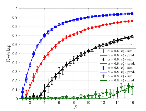
Figure 3: Spectral estimators for noiseless mixed linear regression, with mixing parameter $\alpha\in\{0.6,0.8\}$. Optimal spectral estimators given by Equation 3.35 are used. Overlaps with both signals $x_{1}^{*},x_{2}^{*}$, computed from simulation (“sim.”) and prediction (“pred.”), are plotted as a function of the aspect ratio $\delta$. Same numerics apply to noiseless phase retrieval (see Remark 3.10).

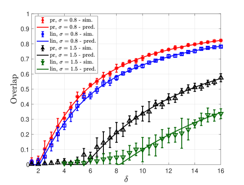
Figure 4: Spectral estimators for mixed linear regression and mixed phase retrieval, with mixing parameter $\alpha=0.8$ and standard deviation of the noise $\sigma\in\{0.8,1.5\}$. Optimal spectral estimators (Equations 3.31 and 3.34) are used. Overlap with the first signal $x_{1}^{*}$, computed from simulation (“sim.”) and prediction (“pred.”), is plotted as a function of the aspect ratio $\delta$.

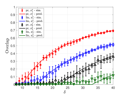
Figure 5: Spectral estimators for mixed linear regression and mixed phase retrieval, with fixed mixing parameter $\alpha=0.6$ and fixed standard deviation of the noise $\sigma=1.5$. Optimal spectral estimators (Equations 3.31 and 3.34) are used. Overlaps with both signals $x_{1}^{*},x_{2}^{*}$, computed from simulation (“sim.”) and prediction (“pred.”), are plotted as a function of the aspect ratio $\delta$.

5 Eigenvalues via random matrix theory

The characterization of the limiting joint law of spectral and linear estimators in Theorem 3.1 is based on the analysis of a Generalized Approximate Message Passing (GAMP) algorithm. The proof of convergence of GAMP to the desired high-dimensional limit, whenever the conditions $\lambda^{*}(\delta_{1})>\overline{\lambda}(\delta)$ and/or $\lambda^{*}(\delta_{2})>\overline{\lambda}(\delta)$ are satisfied, crucially relies on the existence of an eigengap. In this section, we derive the limits of the top three eigenvalues of the matrix $D$ defined in Equation 2.5. This result, stated as Theorem 5.1 below, is then used in Section 6 to prove Theorem 3.1.

Theorem 5.1 (Eigenvalues).

Consider the setting of Section 2.2 and let Items (A1), (A2), (A3), (A4), (A5) and (A7) hold. Then we have

$$\lim_{d\to\infty}\lambda_{1}(D) =\zeta(\lambda^{*}(\delta_{1});\delta),\quad\lim_{d\to\infty}\lambda_{2}(D)=\zeta(\lambda^{*}(\delta_{2});\delta),\quad\lim_{d\to\infty}\lambda_{3}(D)=\zeta(\overline{\lambda}(\delta);\delta),$$

almost surely. Furthermore,

1. If $\lambda^{*}(\delta_{1})>\lambda^{*}(\delta_{2})>\overline{\lambda}(\delta)$, then

   $$\zeta(\lambda^{*}(\delta_{1});\delta)>\zeta(\lambda^{*}(\delta_{2});\delta)>\zeta(\overline{\lambda}(\delta);\delta);$$

2. If $\lambda^{*}(\delta_{1})>\overline{\lambda}(\delta)\geq\lambda^{*}(\delta_{2})$, then

   $$\zeta(\lambda^{*}(\delta_{1});\delta)>\zeta(\lambda^{*}(\delta_{2});\delta)=\zeta(\overline{\lambda}(\delta);\delta);$$

3. If $\overline{\lambda}(\delta)\geq\lambda^{*}(\delta_{1})>\lambda^{*}(\delta_{2})$, then

   $$\zeta(\lambda^{*}(\delta_{1});\delta)=\zeta(\lambda^{*}(\delta_{2});\delta)=\zeta(\overline{\lambda}(\delta);\delta).$$

Remark 5.1 (Phase transition for eigenvalues).

Theorem 5.1 shows a phase transition phenomenon for the top three eigenvalues of $D$: (i) the top two eigenvalues escape from the bulk of $D$ if $\lambda^{*}(\delta_{1})>\lambda^{*}(\delta_{2})>\overline{\lambda}(\delta)$; (ii) only the largest eigenvalue escapes from the bulk if $\lambda^{*}(\delta_{1})>\overline{\lambda}(\delta)\geq\lambda^{*}(\delta_{2})$; (iii) no outlier eigenvalue exists if $\overline{\lambda}(\delta)\geq\lambda^{*}(\delta_{1})>\lambda^{*}(\delta_{2})$. See Figure 2. In words, the condition $\lambda^{*}(\delta_{i})>\overline{\lambda}(\delta)$ is necessary and sufficient for the $i$-th eigenvalue to escape the bulk of the spectrum. This provides an additional piece of evidence (see also Remark 3.7) suggesting that such condition is also necessary and sufficient for the corresponding eigenvector to have non-vanishing overlap with the signal. In fact, phase transitions in the behavior of eigenvalues typically correspond to phase transitions in the behavior of the related eigenvectors, see e.g. [BGN11, BGN12, MM19, LL20].

Remark 5.2 (Eigenvalues for $\alpha=1/2$).

Similar results to Theorem 5.1 hold for $\alpha=1/2$. In this case, the limits of the first and second eigenvalues of $D$ coincide and equal $\zeta(\lambda^{*}(\delta/2);\delta)$. The limit of the right edge of the bulk of $D$ does not depend on $\alpha$ and remains the same ($\overline{\lambda}(\delta)$) as in Theorem 5.1. Therefore, we get two cases: (i) if $\lambda^{*}(\delta/2)>\overline{\lambda}(\delta)$, the top two eigenvalues of $D$ are repeated outliers; otherwise, (ii) $\overline{\lambda}(\delta)\geq\lambda^{*}(\delta/2)$ and there is no outlier eigenvalue in the limiting spectrum of $D$.

Remark 5.3 (Explicit formulas).

By the definition of $\zeta(\lambda;\delta)$ (cf. Equation 3.4), we can write the limits of the eigenvalues in the following more explicit form, which will be convenient in Section 6:

$$\zeta(\lambda^{*}(\delta_{1});\delta) =\begin{cases}\lambda^{*}(\delta_{1})\left(\frac{1}{\delta}+\mathbb{E}\left[\frac{Z}{\lambda^{*}(\delta_{1})-Z}\right]\right),&\lambda^{*}(\delta_{1})>\overline{\lambda}(\delta)\\ \overline{\lambda}(\delta)\left(\frac{1}{\delta}+\mathbb{E}\left[\frac{Z}{\overline{\lambda}(\delta)-Z}\right]\right),&\lambda^{*}(\delta_{1})\leq\overline{\lambda}(\delta)\end{cases},$$

$$\zeta(\lambda^{*}(\delta_{2});\delta) =\begin{cases}\lambda^{*}(\delta_{2})\left(\frac{1}{\delta}+\mathbb{E}\left[\frac{Z}{\lambda^{*}(\delta_{2})-Z}\right]\right),&\lambda^{*}(\delta_{2})>\overline{\lambda}(\delta)\\ \overline{\lambda}(\delta)\left(\frac{1}{\delta}+\mathbb{E}\left[\frac{Z}{\overline{\lambda}(\delta)-Z}\right]\right),&\lambda^{*}(\delta_{2})\leq\overline{\lambda}(\delta)\end{cases},$$

$$\zeta(\overline{\lambda}(\delta);\delta) =\overline{\lambda}(\delta)\left(\frac{1}{\delta}+\mathbb{E}\left[\frac{Z}{\overline{\lambda}(\delta)-Z}\right]\right).$$

Proof of Theorem 5.1..

The proof is divided into three steps. Specifically, we first write $D$ as the sum of two asymptotically free spiked random matrices in Section 5.1. Then, the limit of $\lambda_{3}(D)$ is determined in Lemma 5.2. Finally, the limits of $\lambda_{1}(D),\lambda_{2}(D)$ and the monotonicity properties of the limiting eigenvalues in Items 1, 2 and 3 are given by Lemma 5.3. ∎

5.1 Reduction to free additive convolution

To begin with, assume for notational convenience that $\eta_{i}=1$ for $1\leq i\leq n_{1}$ and $\eta_{i}=0$ for $n_{1}+1\leq i\leq n$, for some $0\leq n_{1}\leq n$. Let $n_{2}=n-n_{1}$. We have almost surely $n_{1}/d\to\delta_{1},n_{2}/d\to\delta_{2}$ since the mixing variables are independent and Bernoulli-distributed with mean $\alpha$. We can write the matrices of interest in block forms

$$A =\begin{bmatrix}A_{1}\\ A_{2}\end{bmatrix},\quad T=\begin{bmatrix}T_{1}&0_{n_{1}\times n_{2}}\\ 0_{n_{2}\times n_{1}}&T_{2}\end{bmatrix},$$ (5.1)

where $A_{1}\in{\mathbb{R}}^{n_{1}\times d},A_{2}\in{\mathbb{R}}^{n_{2}\times d}$ and $T_{1}\in{\mathbb{R}}^{n_{1}\times n_{1}},T_{2}\in{\mathbb{R}}^{n_{2}\times n_{2}}$. We also let ${\underline{\varepsilon}}_{1}=(\varepsilon_{1},\cdots,\varepsilon_{n_{1}})$ and ${\underline{\varepsilon}}_{2}=(\varepsilon_{n_{1}+1},\cdots,\varepsilon_{n})$. Then,

$$A^{\top}TA =\begin{bmatrix}A_{1}^{\top}&A_{2}^{\top}\end{bmatrix}\begin{bmatrix}T_{1}&0_{n_{1}\times n_{2}}\\ 0_{n_{2}\times n_{1}}&T_{2}\end{bmatrix}\begin{bmatrix}A_{1}\\ A_{2}\end{bmatrix}=A_{1}^{\top}T_{1}A_{1}+A_{2}^{\top}T_{2}A_{2}.$$ (5.2)

Note that, for $i\in\{1,2\}$,

$$A_{i}^{\top}T_{i}A_{i} =A_{i}^{\top}\mathrm{diag}({\mathcal{T}}(q(A_{i}x_{i}^{*},{\underline{\varepsilon}}_{i})))A_{i}.$$

Since $A_{1},x_{1}^{*},{\underline{\varepsilon}}_{1}$ and $A_{2},x_{2}^{*},{\underline{\varepsilon}}_{2}$ are mutually independent, we know that $A_{1}^{\top}T_{1}A_{1}$ is independent of $A_{2}^{\top}T_{2}A_{2}$. However, $A_{1}$ and $T_{1}$ are not independent, neither are $A_{2}$ and $T_{2}$.

Let $O\sim\operatorname{Haar}({\mathbb{O}}(d))$ be a matrix sampled uniformly from the orthogonal group ${\mathbb{O}}(d)$ and independent of everything else. Then, we have

$$A_{1}^{\top}T_{1}A_{1}+A_{2}^{\top}T_{2}A_{2} =A_{1}^{\top}\mathrm{diag}({\mathcal{T}}(q(A_{1}x_{1}^{*},{\underline{\varepsilon}}_{1})))A_{1}+A_{2}^{\top}\mathrm{diag}({\mathcal{T}}(q(A_{2}x_{2}^{*},{\underline{\varepsilon}}_{2})))A_{2}$$

$$\overset{\mathrm{d}}{=}A_{1}^{\top}\mathrm{diag}({\mathcal{T}}(q(A_{1}x_{1}^{*},{\underline{\varepsilon}}_{1})))A_{1}+(A_{2}O)^{\top}\mathrm{diag}({\mathcal{T}}(q((A_{2}O)x_{2}^{*},{\underline{\varepsilon}}_{2})))(A_{2}O)$$ (5.3)

$$=A_{1}^{\top}\mathrm{diag}({\mathcal{T}}(q(A_{1}x_{1}^{*},{\underline{\varepsilon}}_{1})))A_{1}+O^{\top}A_{2}^{\top}\mathrm{diag}({\mathcal{T}}(q(A_{2}(Ox_{2}^{*}),{\underline{\varepsilon}}_{2})))A_{2}O$$

$$\overset{\mathrm{d}}{=}A_{1}^{\top}\mathrm{diag}({\mathcal{T}}(q(A_{1}x_{1}^{*},{\underline{\varepsilon}}_{1})))A_{1}+O^{\top}A_{2}^{\top}\mathrm{diag}({\mathcal{T}}(q(A_{2}x_{2}^{*},{\underline{\varepsilon}}_{2})))A_{2}O$$ (5.4)

$$=A_{1}^{\top}T_{1}A_{1}+O^{\top}A_{2}^{\top}T_{2}A_{2}O.$$

Equation 5.3 follows from the independence of $A_{1},A_{2}$, and from the rotational invariance of isotropic Gaussians. Equation 5.4 follows since $O$ and $Ox_{2}^{*}$ are independent if $O\sim\operatorname{Haar}({\mathbb{O}}(d))$ and $x_{2}^{*}\sim\operatorname{Unif}({\mathbb{S}}^{d-1})$. In this step, we crucially use the assumption that $x_{1}^{*}$ and $x_{2}^{*}$ are independent and each uniformly distributed over ${\mathbb{S}}^{d-1}$.

Now $A_{1}^{\top}T_{1}A_{1}$ and $O^{\top}A_{2}^{\top}T_{2}A_{2}O$ are asymptotically free. (See Appendix F for a definition of asymptotic freeness and a primer on free probability theory.) Therefore, we can study $A_{1}^{\top}T_{1}A_{1}$ and $A_{2}^{\top}T_{2}A_{2}$ separately by using existing results, and then apply tools from free probability theory to characterize their sum. In particular, to understand $A_{i}^{\top}T_{i}A_{i}$ for $i\in\{1,2\}$, we use a theorem from [MM19] (transcribed in Theorem I.6); to understand $A_{1}^{\top}T_{1}A_{1}+A_{2}^{\top}T_{2}A_{2}$, we use a theorem from [BBCF17] (transcribed in Theorem G.1).

5.2 Right edge of the bulk of $D$

Before proceeding to the analysis, let us introduce some more notation. Let

$$D_{1}=\frac{1}{n}A_{1}^{\top}T_{1}A_{1},\quad D_{2}=\frac{1}{n}A_{2}^{\top}T_{2}A_{2}.$$ (5.5)

Therefore $D=D_{1}+D_{2}$ according to Equation 5.2. We first calculate the limiting value of the right edge of the bulk of the spectrum of $D$.

Lemma 5.2.

Consider the setting of Section 2.2 and let Items (A1), (A2), (A3), (A4), (A5) and (A7) hold. Denote by $\mu_{D}$ the empirical spectral distribution of $D$. Then

$$\lim_{d\to\infty}\sup\operatorname{supp}(\mu_{D}) =\frac{1}{\delta}\cdot s^{-1}_{\mu_{1}\boxplus\mu_{2}}(-1/\overline{\lambda}(\delta)),$$ (5.6)

almost surely, where $\overline{\lambda}(\delta)$ is the solution to

$$\mathbb{E}\left[\left(\frac{Z}{\overline{\lambda}(\delta)-Z}\right)^{2}\right] =\frac{1}{\delta}$$ (5.7)

and the function $s_{\mu_{1}\boxplus\mu_{2}}^{-1}$ is defined as

$$s_{\mu_{1}\boxplus\mu_{2}}^{-1}(z) =-\frac{1}{z}+\delta\,\mathbb{E}\left[\frac{Z}{1+zZ}\right].$$ (5.8)

Remark 5.4.

The function $s_{\mu_{1}\boxplus\mu_{2}}^{-1}$ is in fact the inverse Stieltjes transform of the free additive convolution of the limiting spectral distributions $\mu_{1}$ of $\frac{n}{d}D_{1}$ and $\mu_{2}$ of $\frac{n}{d}D_{2}$. The function $s_{\mu_{1}\boxplus\mu_{2}}^{-1}(\lambda)$ is tightly connected to the function $\psi(\lambda;\delta)$ defined in Equation 3.2. Indeed, $\frac{1}{\delta}\cdot s_{\mu_{1}\boxplus\mu_{2}}^{-1}(-1/\lambda)$ is precisely $\psi(\lambda;\delta)$. We note also that the parameter $\overline{\lambda}(\delta)$ defined in Equation 5.7 is the same as that defined through Equation 3.3. (See Lemma I.3.) The connection shall become more transparent in the proof below.

Proof of Lemma 5.2.

First note that the scaling factor $\frac{1}{d}$ in Theorem I.7 (which will be used momentarily) is different from our scaling $\frac{1}{n}$ in the definition of $D$ (cf. Equation 2.5). We therefore consider $\widetilde{D}=\frac{1}{d}A^{\top}TA$ for the convenience of applying Theorem I.7. All results regarding the matrix $\widetilde{D}$ can be translated to $D$ by inserting a factor $\frac{d}{n}\to\frac{1}{\delta}$ at proper places, since $D=\frac{d}{n}\widetilde{D}$.

Let

$$\widetilde{D}_{1}=\frac{1}{d}A_{1}^{\top}T_{1}A_{1},\quad\widetilde{D}_{2}=\frac{1}{d}A_{2}^{\top}T_{2}A_{2}.$$ (5.9)

By Equation 5.2, $\widetilde{D}=\widetilde{D}_{1}+\widetilde{D}_{2}$. Let $\mu_{1}$ and $\mu_{2}$ be the limiting spectral distributions of $\widetilde{D}_{1}$ and $\widetilde{D}_{2}$, respectively, as $n_{1},n_{2},d\to\infty$ with $n_{1}/d\to\delta_{1}=\alpha\delta$ and $n_{2}/d\to\delta_{2}=(1-\alpha)\delta$. As argued in Section 5.1, $\widetilde{D}_{1}$ and $\widetilde{D}_{2}$ are asymptotically free. Hence, the limiting spectral distribution of $\widetilde{D}$ is given by the free additive convolution of $\mu_{1},\mu_{2}$, denoted by $\mu_{1}\boxplus\mu_{2}$ [Voi91, Spe93]. It remains to compute $\sup\operatorname{supp}(\mu_{1}\boxplus\mu_{2})$.

A careful inspection of the proof of [MM19, Lemma 2] shows that the bulk of the spectrum of $\widetilde{D}_{i}$ (for $i\in\{1,2\}$ respectively), i.e., $\lambda_{2}(\widetilde{D}_{i})\geq\cdots\geq\lambda_{d}(\widetilde{D}_{i})$, interlaces the spectrum of $E_{i}\coloneqq\frac{1}{d}\widetilde{A}_{i}^{\top}T_{i}\widetilde{A}_{i}\in{\mathbb{R}}^{(d-1)\times(d-1)}$ for $i\in\{1,2\}$, respectively. Specifically,

$$\lambda_{1}(E_{i})\geq\lambda_{2}(\widetilde{D}_{i})\geq\lambda_{2}(E_{i})\geq\lambda_{3}(\widetilde{D}_{i})\geq\cdots\geq\lambda_{d-2}(E_{i})\geq\lambda_{d-1}(\widetilde{D}_{i})\geq\lambda_{d-1}(E_{i})\geq\lambda_{d}(\widetilde{D}_{i}).$$ (5.10)

Here, $T_{i}=\mathrm{diag}({\mathcal{T}}(q(A_{i}x_{i}^{*},{\underline{\varepsilon}}_{i})))$ (recall Equation 5.1) and $\widetilde{A}_{i}\in{\mathbb{R}}^{n_{i}\times(d-1)}$ is an independent matrix with i.i.d. ${\mathcal{N}}(0,1)$ entries. In particular, $T_{i}$ and $\widetilde{A}_{i}$ are independent. For the convenience of applying Theorem I.7, we also define, for $i\in\{1,2\}$, $\widetilde{E}_{i}\coloneqq\frac{1}{d-1}\widetilde{A}_{i}^{\top}T_{i}\widetilde{A}_{i}$. Note that $E_{i}=\frac{d-1}{d}\widetilde{E}_{i}$. Also $n_{1}/(d-1)\to\delta_{1}$ and $n_{2}/(d-1)\to\delta_{2}$.

Since each $y_{i}$ (for $1\leq i\leq n$) is i.i.d., the limiting spectral distributions of $T_{1}$ and $T_{2}$ are in fact the same and both equal the law of $Z$. Thus, Theorem I.7 provides us with a characterization of the limiting spectral distribution of $\widetilde{E}_{i}$:

$$\mu_{\widetilde{E}_{1}} \to\widetilde{\mu}_{1},\quad\mu_{\widetilde{E}_{2}}\to\widetilde{\mu}_{2},$$

weakly as $n_{1},n_{2},d\to\infty$ with $n_{1}/(d-1)\to\delta_{1},n_{2}/(d-1)\to\delta_{2}$. Furthermore, the limiting spectral distributions admit the following explicit description through the inverse Stieltjes transform (see Equation F.1 in Appendix F for the definition of Stieltjes transform of a distribution):

$$s_{\widetilde{\mu}_{1}}^{-1}(z) =-\frac{1}{z}+\delta_{1}\mathbb{E}\left[\frac{Z}{1+zZ}\right],\quad s_{\widetilde{\mu}_{2}}^{-1}(z)=-\frac{1}{z}+\delta_{2}\mathbb{E}\left[\frac{Z}{1+zZ}\right].$$ (5.11)

In view of the scaling factor $\frac{d-1}{d}\to 1$, the limiting spectral distributions of $E_{1},E_{2}$ are also given by $\widetilde{\mu}_{1},\widetilde{\mu}_{2}$, respectively. Recall that the bulks of the spectra of $\widetilde{D}_{1},\widetilde{D}_{2}$ interlace the spectra of $E_{1},E_{2}$, respectively (cf. Equation 5.10). Since $\widetilde{D}_{1}$ and $\widetilde{D}_{2}$ can each have at most one outlier eigenvalue (cf. Theorem I.6), the limiting spectral distributions $\mu_{1},\mu_{2}$ of $\widetilde{D}_{1},\widetilde{D}_{2}$, respectively, are the same as $\widetilde{\mu}_{1},\widetilde{\mu}_{2}$ whose inverse Stieltjes transforms are shown in Equation 5.11.

The following two well-known facts in free probability theory (cf. Equations F.2 and F.3 in Appendix F)

$$R_{\mu_{1}\boxplus\mu_{2}}(z) =R_{\mu_{1}}(z)+R_{\mu_{2}}(z),$$

and

$$R_{\mu}(z) =s_{\mu}^{-1}(-z)-\frac{1}{z},$$

then allows us to compute $s_{\mu_{1}\boxplus\mu_{2}}^{-1}$. Indeed

$$s_{\mu_{1}\boxplus\mu_{2}}^{-1}(z) =s_{\mu_{1}}^{-1}(z)+s_{\mu_{2}}^{-1}(z)+\frac{1}{z}=s_{\widetilde{\mu}_{1}}^{-1}(z)+s_{\widetilde{\mu}_{2}}^{-1}(z)+\frac{1}{z}=-\frac{1}{z}+\delta\mathbb{E}\left[\frac{Z}{1+zZ}\right].$$ (5.12)

Given $s_{\mu_{1}\boxplus\mu_{2}}^{-1}$, one can calculate $\sup\operatorname{supp}(\mu_{1}\boxplus\mu_{2})$ which is in turn the limiting value of $\sup\operatorname{supp}(\mu_{\widetilde{D}})$, where $\mu_{\widetilde{D}}$ denotes the empirical spectral distribution of $\widetilde{D}$. This can be accomplished thanks to the results in [BY12, Lemma 3.1] (see also [SC95, Sec. 4]):

$$\lim_{d\to\infty}\sup\operatorname{supp}(\mu_{\widetilde{D}}) =\sup\operatorname{supp}(\mu_{1}\boxplus\mu_{2})$$ (5.13)

$$=\min_{\lambda>\sup\operatorname{supp}(Z)}s_{\mu_{1}\boxplus\mu_{2}}^{-1}(-1/\lambda)$$

$$=\min_{\lambda>\sup\operatorname{supp}(Z)}\lambda+\delta\mathbb{E}\left[\frac{Z}{1-Z/\lambda}\right].$$ (5.14)

The convergence in Equation 5.13 holds almost surely since

$$\mu_{\widetilde{D}} =\mu_{\widetilde{D}_{1}+\widetilde{D}_{2}}\to\mu_{1}\boxplus\mu_{2}$$

weakly [Voi91, Spe93]. To solve the minimization problem in Equation 5.14, we observe that the function $s_{\mu_{1}\boxplus\mu_{2}}^{-1}(-1/\lambda)$ is intimately related to $\psi(\lambda;\delta)$ defined in Equation 3.2:

$$s_{\mu_{1}\boxplus\mu_{2}}^{-1}(-1/\lambda) =\lambda+\delta\mathbb{E}\left[\frac{Z}{1-Z/\lambda}\right]=\delta\lambda\left(\frac{1}{\delta}+\mathbb{E}\left[\frac{Z}{\lambda-Z}\right]\right)=\delta\cdot\psi(\lambda;\delta).$$

Since $\psi(\lambda;\delta)$ is convex in the first argument (cf. Lemma I.2), so is $s_{\mu_{1}\boxplus\mu_{2}}^{-1}(-1/\lambda)$ as a function of $\lambda$. As a result, the minimizer $\overline{\lambda}(\delta)$ of the above minimization problem (Equation 5.14) is the critical point of $s_{\mu_{1}\boxplus\mu_{2}}^{-1}(-1/\lambda)$. That is,

$$\left.\frac{\mathrm{d}}{\mathrm{d}\lambda}s_{\mu_{1}\boxplus\mu_{2}}^{-1}(-1/\lambda)\right|_{\lambda=\overline{\lambda}(\delta)} =1-\delta\mathbb{E}\left[\left(\frac{Z}{\overline{\lambda}(\delta)-Z}\right)^{2}\right]=0,$$

i.e., $\overline{\lambda}(\delta)$ is the solution to the following equation

$$\mathbb{E}\left[\left(\frac{Z}{\overline{\lambda}(\delta)-Z}\right)^{2}\right] =\frac{1}{\delta}.$$ (5.15)

The minimum value of the above minimization problem (Equation 5.14) is therefore

$$s_{\mu_{1}\boxplus\mu_{2}}^{-1}(-1/\overline{\lambda}(\delta)) =\overline{\lambda}(\delta)\left(1+\delta\mathbb{E}\left[\frac{Z}{\overline{\lambda}(\delta)-Z}\right]\right).$$ (5.16)

At this point, we have successfully computed the limiting value of $\sup\operatorname{supp}(\mu_{\widetilde{D}})$. However, recall that the original matrix we are interested in is $D=\frac{d}{n}(\widetilde{D}_{1}+\widetilde{D}_{2})$. Therefore,

$$\lim_{d\to\infty}\sup\operatorname{supp}(\mu_{D}) =\lim_{d\to\infty}\frac{d}{n}\sup\operatorname{supp}(\mu_{\widetilde{D}})=\overline{\lambda}(\delta)\left(\frac{1}{\delta}+\mathbb{E}\left[\frac{Z}{\overline{\lambda}(\delta)-Z}\right]\right),$$

where $\overline{\lambda}(\delta)$ satisfies Equation 5.15. This concludes the proof. ∎

5.3 Outlier eigenvalues of $D$

Finally, we need to understand the outliers in the spectrum of $D$.

Lemma 5.3.

Consider the setting of Section 2.2 and let Items (A1), (A2), (A3), (A4), (A5) and (A7) hold. Let the function $s_{\mu_{1}\boxplus\mu_{2}}^{-1}(-1/\lambda)$ be given by Equation 5.8. Then, the following statements hold.

1. $\lambda^{*}(\delta_{1})>\lambda^{*}(\delta_{2})$;

2. If $\lambda^{*}(\delta_{1})>\lambda^{*}(\delta_{2})>\overline{\lambda}(\delta)$, then $s_{\mu_{1}\boxplus\mu_{2}}^{-1}(-1/\lambda^{*}(\delta_{1}))>s_{\mu_{1}\boxplus\mu_{2}}^{-1}(-1/\lambda^{*}(\delta_{2}))$;

3. For $i\in\{1,2\}$, if $\lambda^{*}(\delta_{i})>\overline{\lambda}(\delta)$, then $s_{\mu_{1}\boxplus\mu_{2}}^{-1}(-1/\lambda^{*}(\delta_{i}))>s_{\mu_{1}\boxplus\mu_{2}}^{-1}(-1/\overline{\lambda}(\delta))$;

4. We have that, almost surely,

   $$\lim_{d\to\infty}\lambda_{1}(D) =\frac{1}{\delta}\cdot s_{\mu_{1}\boxplus\mu_{2}}^{-1}(-1/\max\{\lambda^{*}(\delta_{1}),\overline{\lambda}(\delta)\}),$$ (5.17)

   $$\lim_{d\to\infty}\lambda_{2}(D) =\frac{1}{\delta}\cdot s_{\mu_{1}\boxplus\mu_{2}}^{-1}(-1/\max\{\lambda^{*}(\delta_{2}),\overline{\lambda}(\delta)\}),$$ (5.18)

   $$\lim_{d\to\infty}\lambda_{3}(D) =\frac{1}{\delta}\cdot\sup\operatorname{supp}(\mu_{1}\boxplus\mu_{2})=\frac{1}{\delta}\cdot s_{\mu_{1}\boxplus\mu_{2}}^{-1}(-1/\overline{\lambda}(\delta)).$$ (5.19)

Remark 5.5.

Recalling the definition $\zeta(\lambda;\delta)=\psi(\max\{\lambda,\overline{\lambda}(\delta)\};\delta)$ (cf. Equation 3.4) and the relation $\frac{1}{\delta}\cdot s_{\mu_{1}\boxplus\mu_{2}}^{-1}(-1/\lambda)=\psi(\lambda;\delta)$ (cf. Remark 5.4), we can write the limiting values of $\lambda_{1}(D),\lambda_{2}(D),\lambda_{3}(D)$ in Equations 5.17, 5.18 and 5.19 as

$$\zeta(\lambda^{*}(\delta_{1});\delta)\geq\zeta(\lambda^{*}(\delta_{2});\delta)\geq\zeta(\overline{\lambda}(\delta);\delta),$$ (5.20)

respectively. To see why the above chain of inequalities holds, note that by Item 3 of Lemma 5.3, $\zeta(\lambda^{*}(\delta_{i});\delta)>\zeta(\overline{\lambda}(\delta);\delta)$ if $\lambda^{*}(\delta_{i})>\overline{\lambda}(\delta)$ and $\zeta(\lambda^{*}(\delta_{i});\delta)=\zeta(\overline{\lambda}(\delta);\delta)$ otherwise. So

$$\zeta(\lambda^{*}(\delta_{i});\delta)\geq\zeta(\overline{\lambda}(\delta);\delta)$$ (5.21)

is always true for $i\in\{1,2\}$. Also, by Item 2 of Lemma 5.3, $\zeta(\lambda^{*}(\delta_{1});\delta)\geq\zeta(\lambda^{*}(\delta_{2});\delta)>\zeta(\overline{\lambda}(\delta);\delta)$ if $\lambda^{*}(\delta_{1})\geq\lambda^{*}(\delta_{2})>\overline{\lambda}(\delta)$. If $\lambda^{*}(\delta_{1})\geq\overline{\lambda}(\delta)\geq\lambda^{*}(\delta_{2})$, $\zeta(\lambda^{*}(\delta_{2});\delta)=\zeta(\overline{\lambda}(\delta);\delta)\leq\zeta(\lambda^{*}(\delta_{1});\delta)$ by Equation 5.21. If $\overline{\lambda}(\delta)\geq\lambda^{*}(\delta_{1})\geq\lambda^{*}(\delta_{2})$, $\zeta(\lambda^{*}(\delta_{1});\delta)=\zeta(\lambda^{*}(\delta_{2});\delta)=\zeta(\overline{\lambda}(\delta);\delta)$. All cases have been exhausted in light of Item 1 of Lemma 5.3. In any case,

$$\zeta(\lambda^{*}(\delta_{1});\delta)\geq\zeta(\lambda^{*}(\delta_{2});\delta)$$ (5.22)

holds. Equation 5.20 then follows from Equations 5.21 and 5.22.

Proof of Lemma 5.3..

The proof is divided into three parts. We first explicitly evaluate the theoretical predictions of the limiting values of the top three eigenvalues of $D$ given by Equation G.1 of Theorem G.1. The convergence of the outlier eigenvalues and the right edge of the bulk to the respective predictions is then formally justified in the second part. Finally, several properties concerning the spectral threshold and the limiting eigenvalues are proved in the third part.

Limiting eigenvalues.

To understand the outlier eigenvalues of $D=D_{1}+D_{2}$, we need to first understand the outlier eigenvalues of $D_{1}$ and $D_{2}$ individually. The latter quantities have been characterized by [MM19, Lemma 2] (transcribed in Theorem I.6). To calibrate the scaling, let us define

$$D_{1}^{\prime}\coloneqq\frac{1}{n_{1}}A_{1}^{\top}T_{1}A_{1},\quad D_{2}^{\prime}\coloneqq\frac{1}{n_{2}}A_{2}^{\top}T_{2}A_{2}.$$

Theorem I.6 then applies to the above matrices $D_{1}^{\prime},D_{2}^{\prime}$ and implies that each of $D_{1}^{\prime}$ and $D_{2}^{\prime}$ has a potential outlier eigenvalue $\lambda_{1}(D_{1}^{\prime})$ and $\lambda_{1}(D_{2}^{\prime})$, respectively. As $n_{1},n_{2},d\to\infty$ with $n_{1}/d\to\delta_{1}$ and $n_{2}/d\to\delta_{2}$, they converge almost surely to the following limiting values:

$$\lim_{d\to\infty}\lambda_{1}(D_{1}^{\prime}) =\zeta(\lambda^{*}(\delta_{1});\delta_{1}),\quad\lim_{d\to\infty}\lambda_{1}(D_{2}^{\prime})=\zeta(\lambda^{*}(\delta_{2});\delta_{2}),$$

where $\lambda^{*}(\delta_{1})$ and $\lambda^{*}(\delta_{2})$ are the solutions to

$$\zeta(\lambda^{*}(\delta_{1});\delta_{1}) =\varphi(\lambda^{*}(\delta_{1})),\quad\zeta(\lambda^{*}(\delta_{2});\delta_{2})=\varphi(\lambda^{*}(\delta_{2})),$$

respectively. For $i\in\{1,2\}$, let us assume that $\lambda_{1}(D_{i}^{\prime})$ is indeed an outlier eigenvalue of $D_{i}^{\prime}$, that is, its limiting value $\zeta(\lambda^{*}(\delta_{i});\delta_{i})$ lies outside the bulk of the limiting spectrum of $D_{i}^{\prime}$. According to Theorem I.6, this happens if and only if $\lambda^{*}(\delta_{i})>\overline{\lambda}(\delta_{i})$. In this case, the limiting value of the outlier eigenvalue can be written more explicitly as

$$\zeta(\lambda^{*}(\delta_{i});\delta_{i})=\psi(\lambda^{*}(\delta_{i});\delta_{i})=\lambda^{*}(\delta_{i})\left(\frac{1}{\delta_{i}}+\mathbb{E}\left[\frac{Z}{\lambda^{*}(\delta_{i})-Z}\right]\right),$$ (5.23)

where $\lambda^{*}(\delta_{i})$ is the solution to

$$\mathbb{E}\left[\frac{Z(G^{2}-1)}{\lambda^{*}(\delta_{i})-Z}\right] =\frac{1}{\delta_{i}}.$$ (5.24)

Let us first translate the above result (i.e., Equations 5.23 and 5.24) regarding $D_{1}^{\prime},D_{2}^{\prime}$ to $\widetilde{D}_{1},\widetilde{D}_{2}$ defined in Equation 5.9. Since $n_{1}/d\to\delta_{1},n_{2}/d\to\delta_{2}$ and $\widetilde{D}_{1}=\frac{n_{1}}{d}D_{1}^{\prime},\widetilde{D}_{2}=\frac{n_{2}}{d}D_{2}^{\prime}$, we have that, almost surely,

$$\lim_{d\to\infty}\lambda_{1}(\widetilde{D}_{i}) =\delta_{i}\lambda^{*}(\delta_{i})\left(\frac{1}{\delta_{i}}+\mathbb{E}\left[\frac{Z}{\lambda^{*}(\delta_{i})-Z}\right]\right)=\lambda^{*}(\delta_{i})\left(1+\delta_{i}\mathbb{E}\left[\frac{Z}{\lambda^{*}(\delta_{i})-Z}\right]\right)\eqqcolon\theta_{i},$$

where we have denoted the limiting value of $\lambda_{1}(\widetilde{D}_{i})$ by $\theta_{i}$. In view of the definition of $s_{\mu_{i}}^{-1}$ in Equation 5.11, we recognize that

$$\theta_{i}=s_{\mu_{i}}^{-1}(-1/\lambda^{*}(\delta_{i})).$$ (5.25)

Provided with the individual outlier of $\widetilde{D}_{i}$ (cf. Equation 5.25), we now invoke [BBCF17, Theorem 2.1] (transcribed in Theorem G.1) to determine how an outlier of $\widetilde{D}_{i}$ is mapped to the spectrum of $\widetilde{D}$ by the free additive convolution. According to Theorem G.1, the limiting value, denoted by $\rho_{i}$, of the potential outlier of $\widetilde{D}=\widetilde{D}_{1}+\widetilde{D}_{2}$ resulting from $\theta_{i}$ is given by

$$\rho_{i}\coloneqq w_{i}^{-1}(\theta_{i}),$$ (5.26)

where $w_{1},w_{2}$ are the pair of subordination functions associated with the pair of distributions $\mu_{1},\mu_{2}$.

As the name suggests, $w_{1},w_{2}$ enjoy the following subordination property (cf. [BBCF17, Sec. 3.4.1] or Equation F.4 in Appendix F):

$$s_{\mu_{1}\boxplus\mu_{2}}(z) =s_{\mu_{1}}(w_{1}(z))=s_{\mu_{2}}(w_{2}(z))=\frac{1}{z-(w_{1}(z)+w_{2}(z))}.$$ (5.27)

To understand the value of $\rho_{i}=w_{i}^{-1}(\theta_{i})$ (cf. Equation 5.26), let us compute

$$s_{\mu_{1}\boxplus\mu_{2}}(w_{i}^{-1}(\theta_{i})) =s_{\mu_{i}}(\theta_{i})=-1/\lambda^{*}(\delta_{i}).$$ (5.28)

The first equality is by the subordination property (Equation 5.27) and the second one by the observation in Equation 5.25. Equation 5.28 then gives

$$\rho_{i} =w_{i}^{-1}(\theta_{i})=s_{\mu_{1}\boxplus\mu_{2}}^{-1}(-1/\lambda^{*}(\delta_{i})).$$ (5.29)

To translate the result in Equation 5.29 regarding $\widetilde{D}$ to $D$ defined in Equation 5.5, we simply note that $D=\frac{d}{n}\widetilde{D}$ and $d/n\to 1/\delta$. Therefore, the limiting eigenvalue of $D$ resulting from the outlier eigenvalue of $D_{i}$ is given by

$$\frac{1}{\delta}\cdot\rho_{i}=\frac{1}{\delta}\cdot s_{\mu_{1}\boxplus\mu_{2}}^{-1}(-1/\lambda^{*}(\delta_{i})),$$ (5.30)

almost surely.

Convergence of eigenvalues.

We then formally justify that the right edge of the bulk and the outlier eigenvalues of $D$ indeed converge to the theoretical predictions in Equations 5.6 and 5.30, respectively, as $d\to\infty$, therefore confirming the validity of the latter formulas. Let ${\mathcal{K}}_{0}\coloneqq\operatorname{supp}(\mu_{1}\boxplus\mu_{2})$. For $i\in\{1,2\}$, let ${\mathcal{K}}_{i}$ be the singleton set $\{\rho_{i}\}$ if $\theta_{i}\notin\operatorname{supp}(\mu_{i})$ and $\emptyset$ otherwise. Let ${\mathcal{K}}\coloneqq{\mathcal{K}}_{0}\cup{\mathcal{K}}_{1}\cup{\mathcal{K}}_{2}$. Then the first statement of [BBCF17, Theorem 2.1] (transcribed in Theorem G.1) guarantees that for any $\varepsilon>0$,

$$\Pr\left[\exists d_{0},\,\forall d>d_{0},\,\{\lambda_{i}(\widetilde{D})\}_{i=1}^{d}\subset{\mathcal{K}}_{\varepsilon}\right] =1,$$ (5.31)

where ${\mathcal{K}}_{\varepsilon}$ denotes the $\varepsilon$-enlargement of ${\mathcal{K}}$, i.e.,

$${\mathcal{K}}_{\varepsilon}\coloneqq\left\{\rho\in{\mathbb{R}}:\inf_{\rho^{\prime}\in{\mathcal{K}}}|\rho-\rho^{\prime}|\leq\varepsilon\right\}.$$

In words, Equation 5.31 says that almost surely for every sufficiently large dimension $d$, the spectrum of $\widetilde{D}$ is contained in an arbitrarily small neighbourhood of ${\mathcal{K}}$. Furthermore, suppose $\rho\in{\mathcal{K}}_{1}\cup{\mathcal{K}}_{2}$ and $\rho\notin{\mathcal{K}}_{0}$, that is, $\rho$ is an outlier in the limiting spectrum of $\widetilde{D}$. Assume also that $\varepsilon>0$ is sufficiently small so that $(\rho-2\varepsilon,\rho+2\varepsilon)\cap{\mathcal{K}}=\{\rho\}$. Then

$$\Pr\left[\exists d_{0},\,\forall d>d_{0},\,\left|\{\lambda_{i}(\widetilde{D})\}_{i=1}^{d}\cap(\rho-2\varepsilon,\rho+2\varepsilon)\right|=\mathds{1}{\left\{w_{1}(\rho)=\theta_{1}\right\}}+\mathds{1}{\left\{w_{2}(\rho)=\theta_{2}\right\}}\right] =1.$$ (5.32)

In words, Equation 5.32 says that almost surely for every sufficiently large dimension $d$, the outlier $\theta_{1}$ (resp. $\theta_{2}$) in the limiting spectrum of $\widetilde{D}_{1}$ (resp. $\widetilde{D}_{2}$) is mapped to $w_{1}^{-1}(\theta_{1})$ (resp. $w_{2}^{-1}(\theta_{2})$) in the limiting spectrum of $\widetilde{D}$. Since $D,D_{1},D_{2}$ and $\widetilde{D},\widetilde{D}_{1},\widetilde{D}_{2}$ only differ by a $\delta$ factor, similar statements hold true for $D,D_{1},D_{2}$ as well.

Combining Equations 5.30, 5.31 and 5.32 yields Equations 5.17, 5.18 and 5.19 in Item 4 of Lemma 5.3.

Properties of spectral threshold and limiting eigenvalues.

We identify under what condition $\rho_{i}=w_{i}^{-1}(\theta_{i})$ is an outlier in the limiting spectrum of $\widetilde{D}$. For this to be the case, $\theta_{i}$ is necessarily an outlier in the limiting spectrum of $\widetilde{D}_{i}$, which is assumed in the preceding derivations. As Theorem I.6 guaranteed, a sufficient and necessary condition for this event is $\lambda^{*}(\delta_{i})>\overline{\lambda}(\delta_{i})$. Under the free additive convolution, the outlier $\theta_{i}$ of $\widetilde{D}_{i}$ is then mapped to $w_{i}^{-1}(\theta_{i})$. Let us compare $w_{i}^{-1}(\theta_{i})$ with $\sup\operatorname{supp}(\mu_{1}\boxplus\mu_{2})$, i.e., the right edge of the bulk of the limiting spectral distribution of $\widetilde{D}=\widetilde{D}_{1}+\widetilde{D}_{2}$. The former quantity equals $s_{\mu_{1}\boxplus\mu_{2}}^{-1}(-1/\lambda^{*}(\delta_{i}))$ (as derived in Equation 5.29) and the latter one equals $s_{\mu_{1}\boxplus\mu_{2}}^{-1}(-1/\overline{\lambda}(\delta))$ (see Equation 5.16 in the proof of Lemma 5.2). Recall the following two facts:

1. $s_{\mu_{1}\boxplus\mu_{2}}^{-1}(-1/\lambda)=\delta\cdot\psi(\lambda;\delta)$ (as observed in Remark 5.4);

2. $\psi(\lambda;\delta)$ is convex in $\lambda$ and increasing for $\lambda\in[\overline{\lambda}(\delta),\infty)$ (proved in Lemma I.2).

We therefore conclude that $s_{\mu_{1}\boxplus\mu_{2}}^{-1}(-1/\lambda^{*}(\delta_{i}))>s_{\mu_{1}\boxplus\mu_{2}}^{-1}(-1/\overline{\lambda}(\delta))$ if $\lambda^{*}(\delta_{i})>\overline{\lambda}(\delta)$. This establishes Item 3 of Lemma 5.3. This condition is more stringent than the previous one $\lambda^{*}(\delta_{i})>\overline{\lambda}(\delta_{i})$. This can be seen by inspecting the definitions (see, e.g., Equation I.3 in Lemma I.3) of $\overline{\lambda}(\delta_{i})$ and $\overline{\lambda}(\delta)$:

$$\mathbb{E}\left[\left(\frac{Z}{\overline{\lambda}(\delta)-Z}\right)^{2}\right] =\frac{1}{\delta},\quad\mathbb{E}\left[\left(\frac{Z}{\overline{\lambda}(\delta_{i})-Z}\right)^{2}\right]=\frac{1}{\delta_{i}},$$ (5.33)

respectively, and realizing that $\overline{\lambda}(\delta)>\overline{\lambda}(\delta_{i})$ since $\delta>\delta_{i}$.

We pause and make the following remark regarding the effect of the free additive convolution on the outliers in the spectra of the addends. Comparing Equation 5.29 with the limiting value of the right edge of the bulk (cf. Equation 5.16), we note the following: $\lambda_{1}(\widetilde{D}_{i})$ being an outlier eigenvalue of $\widetilde{D}_{i}$ does not imply that its image $\rho_{i}$ under the free additive convolution is also an outlier eigenvalue of $\widetilde{D}=\widetilde{D}_{1}+\widetilde{D}_{2}$. In fact, it can be buried strictly inside the bulk, which happens if $\overline{\lambda}(\delta_{i})<\lambda^{*}(\delta_{i})<\overline{\lambda}(\delta)$.

We then show $\lambda^{*}(\delta_{1})>\lambda^{*}(\delta_{2})$ in Item 1 of Lemma 5.3. Recall that $\lambda^{*}(\delta_{1})$ and $\lambda^{*}(\delta_{2})$ are the unique solutions to $\zeta(\lambda^{*}(\delta_{1});\delta_{1})=\varphi(\lambda^{*}(\delta_{1}))$ and $\zeta(\lambda^{*}(\delta_{2});\delta_{2})=\varphi(\lambda^{*}(\delta_{2}))$, respectively. Since $\zeta(\cdot;\delta_{1}),\zeta(\cdot;\delta_{2})$ are non-decreasing and $\varphi(\cdot)$ is strictly decreasing, it suffices to show

$$\zeta(\lambda;\delta_{1})<\zeta(\lambda;\delta_{2})$$ (5.34)

for any $\lambda>\sup\operatorname{supp}(Z)$. We do so in four steps. (The following arguments are best understood with Figure 2 in mind.)

1. First we claim that $\overline{\lambda}(\delta_{1})>\overline{\lambda}(\delta_{2})$. This follows from a similar observation as in Equation 5.33 and the assumption $\alpha>1/2$ (cf. Item (A2)) which implies $\delta_{1}>\delta_{2}$.

2. Second we claim that $\psi(\overline{\lambda}(\delta_{1});\delta_{1})<\psi(\overline{\lambda}(\delta_{2});\delta_{2})$. Indeed,

   $$\psi(\overline{\lambda}(\delta_{1});\delta_{1}) <\psi(\overline{\lambda}(\delta_{2});\delta_{1})<\psi(\overline{\lambda}(\delta_{2});\delta_{2}).$$

   The first inequality follows since $\psi(\lambda;\delta_{1})$ is strictly decreasing for $\lambda\leq\overline{\lambda}(\delta_{1})$ (see Item 2 of Lemma I.2) and $\overline{\lambda}(\delta_{1})>\overline{\lambda}(\delta_{2})$ as shown in Item 1 above. The second inequality follows since

   $$\psi(\cdot;\delta_{1})<\psi(\cdot;\delta_{2})$$ (5.35)

   for any $\lambda>\sup\operatorname{supp}(Z)$ (see the definition of $\psi$ in Equation 3.2 and also Item 3 of Lemma I.2). Note that in this step we use $\sup\operatorname{supp}(Z)>0$ in Item (A7). This shows that Equation 5.34 holds for any $\lambda\leq\overline{\lambda}(\delta_{2})$.

3. We then claim that Equation 5.34 holds for any $\lambda\geq\overline{\lambda}(\delta_{1})$. This is because, in this regime, we have

   $$\zeta(\lambda;\delta_{1})=\psi(\lambda;\delta_{1})<\psi(\lambda;\delta_{2})=\zeta(\lambda;\delta_{2})$$

   using the definition of $\zeta(\cdot;\delta_{i})$ (cf. Equation 3.4) and Equation 5.35.

4. Finally, it remains to verify that Equation 5.34 holds for $\overline{\lambda}(\delta_{2})\leq\lambda\leq\overline{\lambda}(\delta_{1})$. Indeed, we have

   $$\zeta(\lambda;\delta_{1}) =\psi(\overline{\lambda}(\delta_{1});\delta_{1})<\psi(\overline{\lambda}(\delta_{2});\delta_{2})<\psi(\lambda;\delta_{2}).$$

   The equality is by definition of $\zeta(\cdot;\delta_{1})$. The first inequality is by Item 2 above. The second inequality follows since $\psi(\cdot;\delta_{2})$ is strictly increasing for $\lambda\geq\overline{\lambda}(\delta_{2})$ (see Item 2 of Lemma I.2).

Combining Items 1, 2, 3 and 4 above then proves Equation 5.34 which implies Item 1 of Lemma 5.3.

Since $\overline{\lambda}(\delta)$ is the (unique) critical point of $s_{\mu_{1}\boxplus\mu_{2}}^{-1}(-1/\lambda)$ which is increasing for $\lambda\geq\overline{\lambda}(\delta)$, Item 2 of Lemma 5.3 then follows.

The proof of the whole lemma is complete. ∎

6 Joint distribution via Generalized Approximate Message Passing

The limiting joint distribution in Theorem 3.1 is obtained via a generalized approximate message passing (GAMP) algorithm whose iterates converge to the top two eigenvectors of $D=A^{\top}TA$. Within this section, we adopt the following rescaling for the convenience of applying the GAMP machinery:

$$\overline{A} \coloneqq\frac{1}{\sqrt{d}}\,A,\quad\overline{x}_{1}^{*}\coloneqq\sqrt{d}\,x_{1}^{*},\quad\overline{x}_{2}^{*}\coloneqq\sqrt{d}\,x_{2}^{*},\quad\overline{D}\coloneqq\overline{A}^{\top}\,T\,\overline{A}=\frac{n}{d}A^{\top}TA.$$ (6.1)

According to Items (A1) and (A4), we have $\overline{A}_{i,j}\overset{\mathrm{i.i.d.}}{\sim}{\mathcal{N}}(0,1/d)$ and $\overline{x}_{1}^{*},\overline{x}_{2}^{*}\overset{\mathrm{i.i.d.}}{\sim}\operatorname{Unif}(\sqrt{d}\,{\mathbb{S}}^{d-1})$. Let the $i$-th row of $\overline{A}$ be denoted by $\overline{a}_{i}^{\top}\in{\mathbb{R}}^{d}$. Then, we have

$$y_{i} =q\left(\left\langle a_{i},\eta_{i}x_{1}^{*}+(1-\eta_{i})x_{2}^{*}\right\rangle,\varepsilon_{i}\right)=q\left(\left\langle\overline{a}_{i},\eta_{i}\overline{x}_{1}^{*}+(1-\eta_{i})\overline{x}_{2}^{*}\right\rangle,\varepsilon_{i}\right).$$

Therefore, $y\in{\mathbb{R}}^{n}$ and related quantities such as $T\in{\mathbb{R}}^{n\times n}$ (defined in Equation 2.5) do not have to be rescaled. The overlaps are invariant under rescaling of $D$. Furthermore, since $n/d\to\delta$, the limiting eigenvalues of $\overline{D}$ are equal to those of $D$ multiplied by $\delta$ in view of Equation 6.1. The results to be proved in this section will therefore be consistent with those stated in Theorem 3.1.

We first extend the GAMP algorithm for the non-mixed GLM [Ran11] and its associated state evolution analysis to the mixed GLM model. The GAMP algorithm is defined in terms of a sequence of Lipschitz functions $g_{t}:\mathbb{R}^{2}\to\mathbb{R}$ and $f_{t+1}:\mathbb{R}^{3}\to\mathbb{R}$, for $t\geq 0$. For $t\geq 0$, the algorithm iteratively computes $u^{t},{\tilde{u}}^{t}\in{\mathbb{R}}^{n}$ and $v^{t+1},{\tilde{v}}^{t+1}\in{\mathbb{R}}^{d}$ as follows:

$$\begin{split}u^{t}&=\frac{1}{\sqrt{\delta}}\overline{A}{\tilde{v}}^{t}-{\sf b}_{t}{\tilde{u}}^{t-1},\quad{\tilde{u}}^{t}=g_{t}(u^{t};y),\\ v^{t+1}&=\frac{1}{\sqrt{\delta}}\overline{A}^{\top}{\tilde{u}}^{t}-{\sf c}_{t}{\tilde{v}}^{t},\quad{\tilde{v}}^{t+1}=f_{t+1}(v^{t+1};\,\overline{x}_{1}^{*},\overline{x}_{2}^{*}).\end{split}$$ (6.2)

The iteration is initialized with a given ${\tilde{v}}^{0}\in{\mathbb{R}}^{d}$ and ${\tilde{u}}^{-1}=0_{n}$. The functions $f_{t}$ and $g_{t}$ are applied component-wise, i.e., $f_{t}(v^{t};\,\overline{x}_{1}^{*},\overline{x}_{2}^{*})=(f_{t}(v^{t}_{1};\,\overline{x}_{1,1}^{*},\overline{x}_{2,1}^{*})$, $\ldots,f_{t}(v^{t}_{d};\,\overline{x}_{1,d}^{*},\overline{x}_{2,d}^{*}))$ and $g_{t}(u^{t};y)=(g_{t}(u^{t}_{1};y_{1}),\ldots,g_{t}(u^{t}_{n};y_{n}))$. The scalars ${\sf b}_{t},{\sf c}_{t}$ are defined as

$${\sf b}_{t}=\frac{1}{n}\sum_{i=1}^{d}f_{t}^{\prime}(v_{i}^{t};\,\overline{x}_{1,i}^{*},\overline{x}_{2,i}^{*}),\qquad{\sf c}_{t}=\frac{1}{n}\sum_{i=1}^{n}g_{t}^{\prime}(u_{i}^{t};y_{i}),$$ (6.3)

where $f_{t}^{\prime}$ and $g_{t}^{\prime}$ each denote the derivative with respect to the first argument.

An important feature of the GAMP algorithm is that as $d\to\infty$, the empirical distributions of the iterates $u^{t}$ and $v^{t+1}$ converge to the laws of well-defined scalar random variables $U_{t}$ and $V_{t+1}$, respectively. Specifically, for $t\geq 0$, let

$$U_{t}\coloneqq\mu_{1,t}G_{1}+\mu_{2,t}G_{2}+W_{U,t},\quad V_{t+1}\coloneqq\chi_{1,t+1}X_{1}+\chi_{2,t+1}X_{2}+W_{V,t+1},$$ (6.4)

where $(G_{1},G_{2},W_{U,t})\sim{\mathcal{N}}(0,1)\otimes{\mathcal{N}}(0,1)\otimes{\mathcal{N}}(0,\sigma_{U,t}^{2})$, and $(X_{1},X_{2},W_{V,t+1})\sim{\mathcal{N}}(0,1)\otimes{\mathcal{N}}(0,1)\otimes{\mathcal{N}}(0,\sigma_{V,t+1}^{2})$. We remark that the independence of $X_{1}$ and $X_{2}$ (and analogously of $G_{1},G_{2}$) follows from the independence of the two signals $\overline{x}_{1}^{*},\overline{x}_{2}^{*}$. In addition, $X_{1},X_{2}\overset{\mathrm{i.i.d.}}{\sim}{\mathcal{N}}(0,1)$ as the signals $\overline{x}_{1}^{*},\overline{x}_{2}^{*}$ are uniformly distributed on the sphere and, hence, their empirical distribution converges to a standard Gaussian. The deterministic coefficients $(\mu_{1,t},\mu_{2,t},\sigma_{U,t},\chi_{1,t+1},\chi_{2,t+1},\sigma_{V,t+1})$ are computed using the following state evolution recursion:

$$\mu_{1,t}=\frac{1}{\sqrt{\delta}}{\mathbb{E}}[X_{1}f_{t}(V_{t};\,X_{1},X_{2})],\quad\mu_{2,t}=\frac{1}{\sqrt{\delta}}{\mathbb{E}}[X_{2}f_{t}(V_{t};\,X_{1},X_{2})],$$ (6.5)

$$\sigma_{U,t}^{2}=\frac{1}{\delta}{\mathbb{E}}[f_{t}(V_{t};\,X_{1},X_{2})^{2}]-\mu_{1,t}^{2}-\mu_{2,t}^{2}\,,$$

$$\chi_{1,t+1}=\sqrt{\delta}\left({\mathbb{E}}[G_{1}g_{t}(U_{t};{\tilde{Y}})]-{\mathbb{E}}[g_{t}^{\prime}(U_{t};{\tilde{Y}})]\mu_{1,t}\right),\quad\chi_{2,t+1}=\sqrt{\delta}\left({\mathbb{E}}[G_{2}g_{t}(U_{t};{\tilde{Y}})]-{\mathbb{E}}[g_{t}^{\prime}(U_{t};{\tilde{Y}})]\mu_{2,t}\right),$$

$$\qquad\sigma_{V,t+1}^{2}={\mathbb{E}}[g_{t}(U_{t};{\tilde{Y}})^{2}].$$

Here the random variable ${\tilde{Y}}$ is given by

$${\tilde{Y}}=q(\eta G_{1}+(1-\eta)G_{2},\,\varepsilon),\text{ where }(G_{1},G_{2},\eta,\varepsilon)\sim{\mathcal{N}}(0,1)\otimes{\mathcal{N}}(0,1)\otimes\text{Bern}(\alpha)\otimes P_{\varepsilon}.$$ (6.6)

The state evolution recursion is initialized in terms of the limiting correlation of the initializer ${\tilde{v}}^{0}$ with each of the signals $\overline{x}_{1}^{*}$ and $\overline{x}_{2}^{*}$. The existence of these limiting correlations is guaranteed by imposing the following condition on ${\tilde{v}}^{0}$:

1. The initializer ${\tilde{v}}^{0}\in{\mathbb{R}}^{d}$ is independent of $\overline{A}$. Furthermore, there exists a Lipschitz $F_{0}:{\mathbb{R}}^{2}\to{\mathbb{R}}$ such that

   $$\lim_{d\to\infty}\frac{\langle{\tilde{v}}^{0},\,\Phi(\overline{x}_{1}^{*},\overline{x}_{2}^{*})\rangle}{d}={\mathbb{E}}[F_{0}(X_{1},X_{2})\Phi(X_{1},X_{2})]\ \text{ almost surely},$$ (6.7)

   for any Lipschitz $\Phi:{\mathbb{R}}^{2}\to{\mathbb{R}}$. Here $X_{1},X_{2}\overset{\mathrm{i.i.d.}}{\sim}{\mathcal{N}}(0,1)$.

This assumption is typical in AMP algorithms [FVRS22], and our initializer for proving Theorem 3.1 will be ${\tilde{v}}^{0}=0_{d}$, which trivially satisfies Item (A8). Item (A8) allows us to initialize the state evolution recursion as:

$$\mu_{1,0}=\frac{1}{\sqrt{\delta}}\lim_{d\to\infty}\frac{\langle\overline{x}_{1}^{*}\,,\,{\tilde{v}}^{0}\rangle}{d}=\frac{1}{\sqrt{\delta}}{\mathbb{E}}[F_{0}(X_{1},X_{2})X_{1}],\ \ \mu_{2,0}=\frac{1}{\sqrt{\delta}}\lim_{d\to\infty}\frac{\langle\overline{x}_{2}^{*}\,,\,{\tilde{v}}^{0}\rangle}{d}=\frac{1}{\sqrt{\delta}}{\mathbb{E}}[F_{0}(X_{1},X_{2})X_{2}],$$

$$\sigma_{U,0}^{2}=\frac{1}{\delta}\lim_{d\to\infty}\frac{\left\|{\tilde{v}}^{0}\right\|_{2}^{2}}{d}-\mu_{1,0}^{2}-\mu_{2,0}^{2}=\frac{1}{\delta}{\mathbb{E}}[F_{0}(X_{1},X_{2})^{2}]-\mu_{1,0}^{2}-\mu_{2,0}^{2}.$$ (6.8)

The sequences of random variables $(W_{U,t})_{t\geq 0}$ and $(W_{V,t+1})_{t\geq 0}$ in Equation 6.4 are each jointly Gaussian with zero mean and the following covariance structure:

$${\mathbb{E}}[W_{U,0}W_{U,t}]=\frac{1}{\delta}{\mathbb{E}}[F_{0}(X_{1},X_{2})\,f_{t}(V_{t};X_{1},X_{2})]-\mu_{1,0}\mu_{1,t}-\mu_{1,0}\mu_{2,t},\qquad t\geq 1,$$ (6.9)

and for $r,t\geq 1$:

$${\mathbb{E}}[W_{V,r}W_{V,t}]={\mathbb{E}}\left[g_{r-1}(U_{r-1};{\tilde{Y}})\,g_{t-1}(U_{t-1};{\tilde{Y}})\right],$$ (6.10)

$${\mathbb{E}}[W_{U,r}W_{U,t}]=\frac{1}{\delta}{\mathbb{E}}[f_{r}(V_{r};\,X_{1},X_{2})f_{t}(V_{t};\,X_{1},X_{2})]-\mu_{1,r}\mu_{1,t}-\mu_{1,r}\mu_{2,t}.$$ (6.11)

Note that for $r=t$ we have ${\mathbb{E}}[W_{U,t}^{2}]=\sigma_{U,t}^{2}$ and ${\mathbb{E}}[W_{V,t+1}^{2}]=\sigma_{V,t}^{2}$.

The state evolution result for the GAMP is stated in terms of pseudo-Lipschitz test functions (see Equation 3.6).

Proposition 6.1 (State evolution).

Consider the setup of Theorem 3.1 and the GAMP iteration in Equation 6.2, with initialization ${\tilde{v}}^{0}$ that satisfies Item (A8). Assume that for $t\geq 0$, the functions $g_{t}:{\mathbb{R}}^{2}\to{\mathbb{R}}$ and $f_{t+1}:{\mathbb{R}}^{3}\to{\mathbb{R}}$ are Lipschitz. Let $g_{1}\coloneqq\overline{A}\overline{x}_{1}^{*},g_{2}\coloneqq\overline{A}\overline{x}_{2}^{*}$. Then, the following holds almost surely for any ${\rm PL}(2)$ function $\Psi:{\mathbb{R}}^{t+3}\to{\mathbb{R}}$, for $t\geq 0$:

$$\lim_{n\to\infty}\frac{1}{n}\sum_{i=1}^{n}\Psi(g_{1,i},g_{2,i},u^{t}_{i},u^{t-1}_{i},\ldots,u^{0}_{i})={\mathbb{E}}[\Psi(G_{1},G_{2},\,U_{t},\,U_{t-1},\,\ldots,U_{0})],$$ (6.12)

$$\lim_{d\to\infty}\frac{1}{d}\sum_{i=1}^{d}\Psi(\overline{x}_{1,i}^{*},\overline{x}_{2,i}^{*},v^{t+1}_{i},v^{t}_{i},\ldots,v^{1}_{i})={\mathbb{E}}[\Psi(X_{1},\,X_{2},\,V_{t+1},\,V_{t},\,\ldots,V_{1})],$$ (6.13)

where the distributions of the random vectors $(G_{1},G_{2},U_{t},\ldots,U_{0})$ and $(X_{1},X_{2},V_{t+1},\ldots,V_{1})$ are given by the state evolution recursion in Equation 6.4 to (6.11).

The proof of the proposition, given in Appendix H, uses a reduction to an abstract AMP recursion with matrix-valued iterates for which a state evolution result was established in [JM13].

The result in Equation 6.13 is equivalent to the statement that the joint empirical distribution of the rows of $(\overline{x}_{1}^{*},\overline{x}_{2}^{*},v^{t},\ldots,v^{1})$ converges in Wasserstein-$2$ distance to the joint law of $(X_{1},X_{2},V_{t},\ldots,V_{1})$ (see [FVRS22, Corollary 7.21]). A similar equivalence holds for the result in Equation 6.12.

Remark 6.1.

The result in Proposition 6.1 also applies to the GAMP algorithm in which the memory coefficients $({\sf b}_{t},{\sf c}_{t})$ in Equation 6.3 are replaced with their deterministic limits $\bar{{\sf b}}_{t},\bar{{\sf c}}_{t}$ computed via state evolution:

$$\bar{{\sf b}}_{t}=\frac{1}{\delta}{\mathbb{E}}[f_{t}^{\prime}(V_{t};\,X_{1},X_{2})],\qquad\bar{{\sf c}}_{t}={\mathbb{E}}[g_{t}^{\prime}(U_{t};{\tilde{Y}})].$$ (6.14)

This equivalence follows from an argument similar to [FVRS22, Remark 4.3].

6.1 GAMP as a method to compute the linear and spectral estimators

Consider the GAMP iteration in Equation 6.2 with the intializer ${\tilde{v}}^{0}=0$, and the following choice of functions:

$$\begin{split}&g_{0}(u^{0};y)=\sqrt{\delta}{\mathcal{L}}(y),\qquad f_{1}(v;\,\overline{x}_{1}^{*},\overline{x}_{2}^{*})=f(\overline{x}_{1}^{*},\overline{x}_{2}^{*}),\\ &g_{t}(u;\,y)=\sqrt{\delta}\,u\,{\mathcal{F}}(y),\quad f_{t+1}(v;\,\overline{x}_{1}^{*},\overline{x}_{2}^{*})=\frac{v}{\beta_{t+1}},\quad t\geq 1,\end{split}$$ (6.15)

where ${\mathcal{F}}:{\mathbb{R}}\to{\mathbb{R}}$ is bounded and Lipschitz, $f:{\mathbb{R}}\to{\mathbb{R}}$ is Lipschitz, and $\beta_{t+1}$ is a constant, defined iteratively for $t\geq 0$ via the state evolution equations below (Equation 6.20). To prove Theorem 3.1, we will consider two different choices for the pair of functions $(f,{\mathcal{F}})$, in terms of the spectral preprocessing function ${\mathcal{T}}$ (see Equations 6.24 and 6.25). Note that the functions $g_{t}$ and $f_{t+1}$ are required to be Lipschitz for $t\geq 0$, which will be ensured by choosing ${\mathcal{F}}$ to be bounded and Lipschitz.

With the above choice of $f_{t},g_{t}$, the memory coefficients in Equation 6.3 are given by

$${\sf c}_{0}={\sf b}_{1}=0,\qquad{\sf c}_{t}=\sqrt{\delta}\cdot\frac{1}{n}\sum_{i=1}^{n}{\mathcal{F}}(y_{i}),\qquad{\sf b}_{t+1}=\frac{1}{\delta\beta_{t+1}}.$$ (6.16)

Replacing the parameter ${\sf c}_{t}$ with its almost sure limit $\bar{{\sf c}}_{t}=\sqrt{\delta}\,{\mathbb{E}}[{\mathcal{F}}({\tilde{Y}})]$, the GAMP iteration becomes

$$\begin{split}&u^{0}=0,\quad v^{1}=\overline{A}^{\top}{\mathcal{L}}(y),\\ &u^{1}=\frac{1}{\sqrt{\delta}}\overline{A}f(\overline{x}_{1}^{*},\overline{x}_{2}^{*}),\quad v^{2}=\frac{1}{\sqrt{\delta}}\overline{A}^{\top}Fu^{1}-\sqrt{\delta}{\mathbb{E}}[{\mathcal{F}}({\tilde{Y}})]f(\overline{x}_{1}^{*},\overline{x}_{2}^{*}),\\ &u^{t}=\frac{1}{\sqrt{\delta}\,\beta_{t}}\left(\overline{A}v^{t}\,-\,Fu^{t-1}\right),\quad v^{t+1}=\overline{A}^{\top}Fu^{t}-\frac{\sqrt{\delta}}{\beta_{t}}\,{\mathbb{E}}[{\mathcal{F}}({\tilde{Y}})]\,v^{t},\qquad t\geq 2,\end{split}$$ (6.17)

where $F=\mathrm{diag}({\mathcal{F}}(y_{1}),\ldots,{\mathcal{F}}(y_{n}))$. With $f_{t},g_{t}$ given by Equation 6.15, the initialization for the state evolution in Equation 6.5 to (6.8) is:

$$\mu_{1,0}=\mu_{2,0}=\sigma_{U,0}^{2}=0,$$

$$\chi_{1,1}=\delta{\mathbb{E}}[G_{1}{\mathcal{L}}({\tilde{Y}})],\quad\chi_{2,1}=\delta{\mathbb{E}}[G_{2}{\mathcal{L}}({\tilde{Y}})],\quad\sigma_{V,1}^{2}=\delta{\mathbb{E}}[{\mathcal{L}}({\tilde{Y}})^{2}],$$

$$\mu_{1,1}=\frac{1}{\sqrt{\delta}}\mathbb{E}\left[X_{1}f(X_{1},X_{2})\right],\quad\mu_{2,1}=\frac{1}{\sqrt{\delta}}\mathbb{E}\left[X_{2}f(X_{1},X_{2})\right],$$

$$\sigma_{U,1}^{2}=\frac{1}{\delta}\mathbb{E}\left[f(X_{1},X_{2})^{2}\right]-\mu_{1,1}^{2}-\mu_{2,1}^{2},$$ (6.18)

where the joint distribution of $(G_{1},G_{2},{\tilde{Y}})$ is given by Equation 6.6. Furthermore, for $t\geq 1$:

$$\chi_{1,t+1}=\delta\mu_{1,t}\,{\mathbb{E}}[{\mathcal{F}}({\tilde{Y}})(G_{1}^{2}-1)],\qquad\chi_{2,t+1}=\delta\mu_{2,t}\,{\mathbb{E}}[{\mathcal{F}}({\tilde{Y}})(G_{2}^{2}-1)],$$

$$\sigma_{V,t+1}^{2}=\delta\left(\mu_{1,t}^{2}{\mathbb{E}}[{\mathcal{F}}({\tilde{Y}})^{2}G_{1}^{2}]+\mu_{2,t}^{2}{\mathbb{E}}[{\mathcal{F}}({\tilde{Y}})^{2}G_{2}^{2}]+\sigma_{U,t}^{2}{\mathbb{E}}[{\mathcal{F}}({\tilde{Y}})^{2}]\right),$$ (6.19)

$$\beta_{t+1}\coloneqq\sqrt{\chi_{1,t+1}^{2}+\chi_{2,t+1}^{2}+\sigma_{V,t+1}^{2}}\,,$$ (6.20)

$$\mu_{1,t+1}=\frac{\chi_{1,t+1}}{\sqrt{\delta}\beta_{t+1}},\qquad\mu_{2,{t+1}}=\frac{\chi_{2,t+1}}{\sqrt{\delta}\beta_{t+1}},\qquad\sigma_{U,t+1}^{2}=\frac{\sigma_{V,t+1}^{2}}{\delta\beta_{t+1}^{2}}.$$ (6.21)

First note that the iterate $v^{1}$ coincides with the linear estimator $\widehat{x}^{\mathrm{lin}}$ in Equation 2.3. We will show that in the high-dimensional limit the iterate $v^{t}$ is aligned with an eigenvector of the matrix $M\coloneqq\overline{A}^{\top}F(\sqrt{\delta}\beta_{\infty}I_{n}+F)^{-1}\overline{A}$, as $t\to\infty$. (Lemma 6.2 shows that $\beta_{\infty}=\lim\limits_{t\to\infty}\beta_{t}$ is well-defined for our choices of ${\mathcal{F}}$ and initializations.) For a heuristic justification of this claim, assume the iterates $u^{t},v^{t}$ converge to the limits $u^{\infty},v^{\infty}$ in the sense that $\lim\limits_{t\to\infty}\lim\limits_{d\to\infty}\frac{1}{d}\left\|u^{t}-u^{\infty}\right\|_{2}^{2}=0$ and $\lim\limits_{t\to\infty}\lim\limits_{d\to\infty}\frac{1}{d}\left\|v^{t}-v^{\infty}\right\|_{2}^{2}=0$. Then, from Equation 6.17 these limits satisfy

$$u^{\infty}=\frac{1}{\sqrt{\delta}\,\beta_{\infty}}\left(\overline{A}v^{\infty}\,-\,Fu^{\infty}\right),\qquad v^{\infty}=\overline{A}^{\top}Fu^{\infty}-\frac{\sqrt{\delta}}{\beta_{\infty}}\,{\mathbb{E}}[{\mathcal{F}}({\tilde{Y}})]\,v^{\infty},$$ (6.22)

which after simplification, can be written as:

$$v^{\infty}\left(1+\frac{\sqrt{\delta}}{\beta_{\infty}}{\mathbb{E}}[{\mathcal{F}}({\tilde{Y}})]\right)=\overline{A}^{\top}F(\sqrt{\delta}\beta_{\infty}I_{n}+F)^{-1}\overline{A}v^{\infty}.$$ (6.23)

Therefore, $v^{\infty}$ is an eigenvector of the matrix $\overline{A}^{\top}F(\sqrt{\delta}\beta_{\infty}I_{n}+F)^{-1}\overline{A}$, and the GAMP iteration Equation 6.17 is effectively a power method.

We wish to obtain via GAMP the two leading eigenvectors of the matrix $\overline{A}^{\top}T\overline{A}$, so the heuristic above indicates that we should choose ${\mathcal{F}}$ so that $F(\sqrt{\delta}\beta_{\infty}I_{n}+F)^{-1}=c\,T$, for some constant $c$. To this end, we analyze the iteration in Equation 6.17 with two choices for the function ${\mathcal{F}}(y)$ and initialization ${\tilde{v}}^{0}$:

$$\text{ Choice 1}:\quad{\mathcal{F}}_{1}(y)\coloneqq\frac{{\mathcal{T}}(y)}{\lambda^{*}(\delta_{1})-{\mathcal{T}}(y)},\quad f(\overline{x}_{1}^{*},\overline{x}_{2}^{*})=\overline{x}_{1}^{*},$$ (6.24)

$$\text{ Choice 2}:\quad{\mathcal{F}}_{2}(y)\coloneqq\frac{{\mathcal{T}}(y)}{\lambda^{*}(\delta_{2})-{\mathcal{T}}(y)},\quad f(\overline{x}_{1}^{*},\overline{x}_{2}^{*})=\overline{x}_{2}^{*}.$$ (6.25)

Here, we recall that, for $i\in\{1,2\}$, $\lambda^{*}(\delta_{i})$ is the unique solution of $\zeta(\lambda;\delta_{i})=\varphi(\lambda)$ (see p. 3). The initializations in Equations 6.24 and 6.25 are not feasible in practice since they depend on the unknown signals $\overline{x}_{1}^{*}$ and $\overline{x}_{2}^{*}$, but this is not an issue as we use the GAMP in Equation 6.15 only as a proof technique.

We now examine the state evolution recursion in Equations 6.19, 6.20 and 6.21 under each of these choices.

Choice 1.

From Equation 6.18, this corresponds to the initialization

$$\chi_{1,1}=\delta{\mathbb{E}}[G_{1}{\mathcal{L}}({\tilde{Y}})],\ \chi_{2,1}=\delta{\mathbb{E}}[G_{2}{\mathcal{L}}({\tilde{Y}})],\ \sigma_{V,1}^{2}=\delta{\mathbb{E}}[{\mathcal{L}}({\tilde{Y}})^{2}],\ \mu_{1,1}=\frac{1}{\sqrt{\delta}},\ \mu_{2,1}=\sigma_{U,1}^{2}=0.$$ (6.26)

For $t\geq 1$, the state evolution equations in Equations 6.19, 6.20 and 6.21 reduce to:

$$\begin{split}&\chi_{1,t+1}=\delta\mu_{1,t}\,{\mathbb{E}}[{\mathcal{F}}_{1}({\tilde{Y}})(G_{1}^{2}-1)],\quad\sigma_{V,t+1}^{2}=\delta\left(\mu_{1,t}^{2}{\mathbb{E}}[{\mathcal{F}}_{1}({\tilde{Y}})^{2}G_{1}^{2}]\,+\,\sigma_{U,t}^{2}{\mathbb{E}}[{\mathcal{F}}_{1}({\tilde{Y}})^{2}]\right),\\ &\beta_{t+1}=\sqrt{\chi_{1,t+1}^{2}+\sigma_{V,t+1}^{2}}\,,\qquad\mu_{1,t+1}=\frac{\chi_{1,t+1}}{\sqrt{\delta}\beta_{t+1}}\,,\qquad\sigma_{U,t+1}^{2}=\frac{\sigma_{V,t+1}^{2}}{\delta\beta_{t+1}^{2}}\,,\\ \end{split}$$ (6.27)

and $\mu_{2,t+1}=\chi_{2,t+1}=0$ for $t\geq 1$. Using this in Proposition 6.1, we obtain that:

$$\lim_{d\to\infty}\frac{{\langle}\overline{x}_{1}^{*},v^{1}{\rangle}}{d}=\chi_{1,1},\;\lim_{d\to\infty}\frac{{\langle}\overline{x}_{2}^{*},v^{1}{\rangle}}{d}=\chi_{2,1},\;\lim_{d\to\infty}\frac{{\langle}\overline{x}_{1}^{*},v^{t+1}{\rangle}}{d}=\chi_{1,t+1},\;\lim_{d\to\infty}\frac{{\langle}\overline{x}_{2}^{*},v^{t+1}{\rangle}}{d}=0,$$ (6.28)

for $t\geq 1$. Thus, when initialized with $f(\overline{x}_{1}^{*},\overline{x}_{2}^{*})=\overline{x}_{1}^{*}$, the GAMP iterates $\{v^{t+1}\}_{t\geq 1}$ are asymptotically uncorrelated with the signal $\overline{x}_{2}^{*}$.

Choice 2.

This corresponds to the initialization

$$\chi_{1,1}=\delta{\mathbb{E}}[G_{1}{\mathcal{L}}({\tilde{Y}})],\ \chi_{2,1}=\delta{\mathbb{E}}[G_{2}{\mathcal{L}}({\tilde{Y}})],\ \sigma_{V,1}^{2}=\delta{\mathbb{E}}[{\mathcal{L}}({\tilde{Y}})^{2}],\ \mu_{2,1}=\frac{1}{\sqrt{\delta}},\ \mu_{1,1}=\sigma_{U,1}^{2}=0.$$ (6.29)

The state evolution equations are: $\mu_{1,t+1}=\chi_{1,t+1}=0$ for $t\geq 1$, and

$$\begin{split}&\chi_{2,t+1}=\delta\mu_{2,t}\,{\mathbb{E}}[{\mathcal{F}}_{2}({\tilde{Y}})(G_{2}^{2}-1)],\quad\sigma_{V,t+1}^{2}=\delta\left(\mu_{2,t}^{2}{\mathbb{E}}[{\mathcal{F}}_{2}({\tilde{Y}})^{2}G_{2}^{2}]\,+\,\sigma_{U,t}^{2}{\mathbb{E}}[{\mathcal{F}}_{2}({\tilde{Y}})^{2}]\right),\\ &\beta_{t+1}=\sqrt{\chi_{2,t+1}^{2}+\sigma_{V,t+1}^{2}}\,,\qquad\mu_{2,t+1}=\frac{\chi_{2,t+1}}{\sqrt{\delta}\beta_{t+1}},\qquad\sigma_{U,t+1}^{2}=\frac{\sigma_{V,t+1}^{2}}{\delta\beta_{t+1}^{2}}\,.\end{split}$$ (6.30)

Using this in Proposition 6.1, we obtain that for $t\geq 1$,

$$\lim_{d\to\infty}\frac{{\langle}\overline{x}_{1}^{*},v^{1}{\rangle}}{d}=\chi_{1,1},\;\lim_{d\to\infty}\frac{{\langle}\overline{x}_{2}^{*},v^{1}{\rangle}}{d}=\chi_{2,1},\;\lim_{d\to\infty}\frac{{\langle}\overline{x}_{1}^{*},v^{t+1}{\rangle}}{d}=0,\;\lim_{d\to\infty}\frac{{\langle}\overline{x}_{2}^{*},v^{t+1}{\rangle}}{d}=\chi_{2,t+1}.$$ (6.31)

The following lemma gives the fixed point of state evolution under choices 1 and 2.

Lemma 6.2 (Limiting values of state evolution parameters).

1. Assume that ${\mathbb{E}}[{\mathcal{F}}_{1}({\tilde{Y}})(G_{1}^{2}-1)]>0$ and $\delta>\frac{{\mathbb{E}}[{\mathcal{F}}_{1}({\tilde{Y}})^{2}]}{({\mathbb{E}}[{\mathcal{F}}_{1}({\tilde{Y}})(G_{1}^{2}-1)])^{2}}$. Then, as $t\to\infty$ the state evolution parameters $(\chi_{1,t},\sigma_{V,t}^{2})$ in Equation 6.27 under choice 1 converge to the fixed point $(\tilde{\chi}_{1},\tilde{\sigma}_{1}^{2})$, where

   $$\tilde{\chi}_{1}=\sqrt{\frac{\tilde{\beta}_{1}^{2}(\tilde{\beta}_{1}^{2}-{\mathbb{E}}[{\mathcal{F}}_{1}({\tilde{Y}})^{2}])}{\tilde{\beta}_{1}^{2}+{\mathbb{E}}[{\mathcal{F}}_{1}({\tilde{Y}})^{2}G_{1}^{2}]-{\mathbb{E}}[{\mathcal{F}}_{1}({\tilde{Y}})^{2}]}},\qquad\tilde{\sigma}_{1}^{2}=\frac{\tilde{\beta}_{1}^{2}{\mathbb{E}}[{\mathcal{F}}_{1}({\tilde{Y}})^{2}G_{1}^{2}]}{\tilde{\beta}_{1}^{2}+{\mathbb{E}}[{\mathcal{F}}_{1}({\tilde{Y}})^{2}G_{1}^{2}]-{\mathbb{E}}[{\mathcal{F}}_{1}({\tilde{Y}})^{2}]},$$ (6.32)

   and

   $$\tilde{\beta}_{1}^{2}=\tilde{\chi}_{1}^{2}+\tilde{\sigma}_{1}^{2}=\delta\,({\mathbb{E}}[{\mathcal{F}}_{1}({\tilde{Y}})(G_{1}^{2}-1)])^{2}.$$ (6.33)

2. Assume that ${\mathbb{E}}[{\mathcal{F}}_{2}({\tilde{Y}})(G_{2}^{2}-1)]>0$ and $\delta>\frac{{\mathbb{E}}[{\mathcal{F}}_{2}({\tilde{Y}})^{2}]}{({\mathbb{E}}[{\mathcal{F}}_{2}({\tilde{Y}})(G_{2}^{2}-1)])^{2}}$. Then, as $t\to\infty$ the state evolution parameters $(\chi_{2,t},\sigma_{V,t}^{2})$ in Equation 6.30 under choice 2 converge to the fixed point $(\tilde{\chi}_{2},\tilde{\sigma}_{2}^{2})$, where

   $$\tilde{\chi}_{2}=\sqrt{\frac{\tilde{\beta}_{2}^{2}(\tilde{\beta}_{2}^{2}-{\mathbb{E}}[{\mathcal{F}}_{2}({\tilde{Y}})^{2}])}{\tilde{\beta}_{2}^{2}+{\mathbb{E}}[{\mathcal{F}}_{2}({\tilde{Y}})^{2}G_{2}^{2}]-{\mathbb{E}}[{\mathcal{F}}_{2}({\tilde{Y}})^{2}]}},\qquad\tilde{\sigma}_{2}^{2}=\frac{\tilde{\beta}_{2}^{2}{\mathbb{E}}[{\mathcal{F}}_{2}({\tilde{Y}})^{2}G_{2}^{2}]}{\tilde{\beta}_{2}^{2}+{\mathbb{E}}[{\mathcal{F}}_{2}({\tilde{Y}})^{2}G_{2}^{2}]-{\mathbb{E}}[{\mathcal{F}}_{2}({\tilde{Y}})^{2}]},$$ (6.34)

   and

   $$\tilde{\beta}_{2}^{2}=\tilde{\chi}_{2}^{2}+\tilde{\sigma}_{2}^{2}=\delta\,({\mathbb{E}}[{\mathcal{F}}_{2}({\tilde{Y}})(G_{2}^{2}-1)])^{2}.$$ (6.35)

Proof.

The proof of each part of the lemma is identical to that of Lemma 5.2 in [MTV21], which analyzes GAMP for a non-mixed GLM with $f_{t},g_{t}$ given by Equation 6.15. The state evolution recursion under choice 1 in Equations 6.26 and 6.27 has the same form for all values of $\alpha\in[1/2,1)$. The value of $\alpha$ affects the recursion only through the joint distribution of $(\widetilde{Y},G_{1})=(q(\eta G_{1}+(1-\eta)G_{2},\varepsilon),G_{1})$, where $\eta\sim\operatorname{Bern}(\alpha)$. The proof of Lemma 5.2 in [MTV21] does not depend on this joint distribution and applies for any $\alpha$ such that the lower bound on $\delta$ in the statement of the first part is satisfied. The argument for part 2 of the lemma is similar: under choice 2, the joint distribution determining the state evolution in Equations 6.29 and 6.30 is $(\widetilde{Y},G_{2})=(q(\eta G_{1}+(1-\eta)G_{2},\varepsilon),G_{2})$. ∎

It is convenient to express the state evolution fixed points in Lemma 6.2 in terms of the joint law of $(G,Y)$, where $Y=q(G,\varepsilon)$, with $G\sim{\mathcal{N}}(0,1)$ and $\varepsilon\sim P_{\varepsilon}$ are independent. Recalling the joint law of $({\tilde{Y}},G_{1},G_{2})$ given in Equation 6.6 and the definitions of ${\mathcal{F}}_{1},{\mathcal{F}}_{2}$ in Equations 6.24 and 6.25, we have

$${\mathbb{E}}[{\mathcal{F}}_{1}({\tilde{Y}})] ={\mathbb{E}}[{\mathcal{F}}_{1}(Y)]={\mathbb{E}}\left[\frac{{\mathcal{T}}(Y)}{\lambda^{*}(\delta_{1})-{\mathcal{T}}(Y)}\right],\quad{\mathbb{E}}[{\mathcal{F}}_{1}({\tilde{Y}})^{2}]={\mathbb{E}}[{\mathcal{F}}_{1}(Y)^{2}]={\mathbb{E}}\left[\frac{{\mathcal{T}}(Y)^{2}}{(\lambda^{*}(\delta_{1})-{\mathcal{T}}(Y))^{2}}\right],$$

$${\mathbb{E}}[{\mathcal{F}}_{1}({\tilde{Y}})G_{1}^{2}] =\alpha{\mathbb{E}}[{\mathcal{F}}_{1}(q(G_{1},\varepsilon))G_{1}^{2}]+(1-\alpha){\mathbb{E}}[{\mathcal{F}}_{1}(q(G_{2},\varepsilon))G_{1}^{2}]$$

$$=\alpha{\mathbb{E}}\left[\frac{{\mathcal{T}}(Y)G^{2}}{\lambda^{*}(\delta_{1})-{\mathcal{T}}(Y)}\right]+(1-\alpha){\mathbb{E}}\left[\frac{{\mathcal{T}}(Y)}{\lambda^{*}(\delta_{1})-{\mathcal{T}}(Y)}\right]$$

$$=\frac{1}{\delta}+{\mathbb{E}}\left[\frac{{\mathcal{T}}(Y)}{\lambda^{*}(\delta_{1})-{\mathcal{T}}(Y)}\right],$$ (6.36)

where the last equality holds because ${\mathbb{E}}\left[\frac{{\mathcal{T}}(Y)(G^{2}-1)}{\lambda^{*}(\delta_{1})-{\mathcal{T}}(Y)}\right]=\frac{1}{\delta_{1}}$ from Equation I.4, and $\delta_{1}=\alpha\delta$. Similarly, we obtain

$${\mathbb{E}}[{\mathcal{F}}_{2}({\tilde{Y}})]={\mathbb{E}}[{\mathcal{F}}_{2}(Y)]{\mathbb{E}}\left[\frac{{\mathcal{T}}(Y)}{\lambda^{*}(\delta_{2})-{\mathcal{T}}(Y)}\right],\quad{\mathbb{E}}[{\mathcal{F}}_{2}({\tilde{Y}})^{2}]={\mathbb{E}}\left[\frac{{\mathcal{T}}(Y)^{2}}{(\lambda^{*}(\delta_{2})-{\mathcal{T}}(Y))^{2}}\right],$$

$${\mathbb{E}}[{\mathcal{F}}_{2}({\tilde{Y}})G_{2}^{2}]=\frac{1}{\delta}+{\mathbb{E}}\left[\frac{{\mathcal{T}}(Y)}{\lambda^{*}(\delta_{2})-{\mathcal{T}}(Y)}\right].$$ (6.37)

Using Equation 6.36, the formulas for ${\tilde{\beta}}_{1}^{2},{\tilde{\beta}}_{2}^{2}$ in Equations 6.33 and 6.35 become:

$${\tilde{\beta}}_{1}^{2}=\delta\left(\alpha{\mathbb{E}}\left[\frac{{\mathcal{T}}(Y)(G^{2}-1)}{\lambda^{*}(\delta_{1})-{\mathcal{T}}(Y)}\right]\right)^{2}=\frac{1}{\delta},\quad{\tilde{\beta}}_{2}^{2}=\delta\left((1-\alpha){\mathbb{E}}\left[\frac{{\mathcal{T}}(Y)(G^{2}-1)}{\lambda^{*}(\delta_{2})-{\mathcal{T}}(Y)}\right]\right)^{2}=\frac{1}{\delta}.$$ (6.38)

We similarly obtain

$$\tilde{\chi}_{1}=\frac{\rho_{1}^{\mathrm{spec}}}{\sqrt{\delta}},\quad\tilde{\sigma}_{1}^{2}=\frac{1-(\rho_{1}^{\mathrm{spec}})^{2}}{\delta},\qquad\tilde{\chi}_{2}=\frac{\rho_{2}^{\mathrm{spec}}}{\sqrt{\delta}},\quad\tilde{\sigma}_{2}^{2}=\frac{1-(\rho_{2}^{\mathrm{spec}})^{2}}{\delta},$$ (6.39)

where $\rho_{1}^{\mathrm{spec}},\rho_{2}^{\mathrm{spec}}$ are defined in Equation 3.5.

Proof heuristic.

Let us revisit the heuristic sanity-check in Equation 6.23. Under choice 1, i.e., with ${\mathcal{F}}={\mathcal{F}}_{1}$, $F=F_{1}\coloneqq\mathrm{diag}({\mathcal{F}}_{1}(y_{1}),\ldots,{\mathcal{F}}_{1}(y_{n}))$, and $\beta_{\infty}=\tilde{\beta}_{1}$, by using the formulas above for $\tilde{\beta}_{1}$ and ${\mathbb{E}}[{\mathcal{F}}_{1}({\tilde{Y}})]$, Equation 6.23 becomes:

$$v^{\infty}\left(1+\delta{\mathbb{E}}\left[\frac{{\mathcal{T}}(Y)}{\lambda^{*}(\delta_{1})-{\mathcal{T}}(Y)}\right]\right)=\overline{A}^{\top}F_{1}(I_{n}+F_{1})^{-1}\overline{A}v^{\infty}=\frac{1}{\lambda^{*}(\delta_{1})}\overline{A}^{\top}T\overline{A}v^{\infty},$$ (6.40)

where we recall that $T=\mathrm{diag}({\mathcal{T}}(y_{1}),\ldots,{\mathcal{T}}(y_{n}))$. Similarly, under choice 2, i.e., with ${\mathcal{F}}={\mathcal{F}}_{2}$, $F=F_{2}\coloneqq\mathrm{diag}({\mathcal{F}}_{2}(y_{1}),\ldots,{\mathcal{F}}_{2}(y_{n}))$, and $\beta_{\infty}=\tilde{\beta}_{2}$, Equation 6.23 gives:

$$v^{\infty}\left(1+\delta{\mathbb{E}}\left[\frac{{\mathcal{T}}(Y)}{\lambda^{*}(\delta_{2})-{\mathcal{T}}(Y)}\right]\right)=\overline{A}^{\top}F_{2}(I_{n}+F_{2})^{-1}\overline{A}v^{\infty}=\frac{1}{\lambda^{*}(\delta_{2})}\overline{A}^{\top}T\overline{A}v^{\infty},$$ (6.41)

Therefore, with choice 1, Equation 6.40 suggests that the GAMP iterate converges to an eigenvector of $\overline{D}=\overline{A}^{\top}T\overline{A}$ corresponding to the eigenvalue $\lambda^{*}(\delta_{1})\left(1+\delta{\mathbb{E}}\left[\frac{{\mathcal{T}}(Y)}{\lambda^{*}(\delta_{1})-{\mathcal{T}}(Y)}\right]\right)$. Similarly, Equation 6.41 suggests that with choice 2, the GAMP iterate converges to an eigenvector of $\overline{D}$ corresponding to the eigenvalue $\lambda^{*}(\delta_{2})\left(1+\delta{\mathbb{E}}\left[\frac{{\mathcal{T}}(Y)}{\lambda^{*}(\delta_{2})-{\mathcal{T}}(Y)}\right]\right)$. Moreover, when $\lambda^{*}(\delta_{1})>\overline{\lambda}(\delta)$, Theorem 5.1 and Remark 5.3 tell us that the leading eigenvalue of $\overline{D}$ converges to:

$$\lambda_{1}(\overline{D})\stackrel{{\scriptstyle d\to\infty}}{{\longrightarrow}}\lambda^{*}(\delta_{1})\left(1+\delta{\mathbb{E}}\left[\frac{{\mathcal{T}}(Y)}{\lambda^{*}(\delta_{1})-{\mathcal{T}}(Y)}\right]\right).$$ (6.42)

Furthermore, when $\lambda^{*}(\delta_{2})>\overline{\lambda}(\delta)$, the second eigenvalue of $\overline{D}$ converges to:

$$\lambda_{2}(\overline{D})\stackrel{{\scriptstyle d\to\infty}}{{\longrightarrow}}\lambda^{*}(\delta_{2})\left(1+\delta{\mathbb{E}}\left[\frac{{\mathcal{T}}(Y)}{\lambda^{*}(\delta_{2})-{\mathcal{T}}(Y)}\right]\right).$$ (6.43)

Therefore, Equations 6.40 and 6.41 indicate that the GAMP iterates under choices 1 and 2 converge to the eigenvectors corresponding to the two largest eigenvalues of $\overline{D}$, when $\lambda^{*}(\delta_{1})>\lambda^{*}(\delta_{2})>\overline{\lambda}(\delta)$. We now make this claim rigorous.

6.2 Proof of Theorem 3.1

Consider the GAMP iteration in Equation 6.17 for $t\geq 2$. By substituting the expression for $u^{t}$ in the $v^{t+1}$ update, the iteration can be rewritten as follows:

$$u^{t} =\frac{1}{\sqrt{\delta}\,\beta_{t}}\left(\overline{A}v^{t}\,-\,Fu^{t-1}\right),\qquad v^{t+1}=\frac{1}{\sqrt{\delta}\beta_{t}}\left[\left(\overline{A}^{\top}F\overline{A}-\delta{\mathbb{E}}[{\mathcal{F}}({\tilde{Y}})]\,I_{d}\right)v^{t}\,-\,\overline{A}^{\top}F^{2}u^{t-1}\right].$$ (6.44)

In the remainder of the proof, we will assume that $t\geq 2$. Define

$$e_{1}^{t} =u^{t}-u^{t-1},$$ (6.45)

$$e_{2}^{t} =v^{t+1}-v^{t}.$$ (6.46)

By combining Equation 6.45 with Equation 6.44, we have

$$u^{t-1}=(F+\sqrt{\delta}\beta_{t}I_{n})^{-1}\overline{A}v^{t}-\sqrt{\delta}\beta_{t}(F+\sqrt{\delta}\beta_{t}I_{n})^{-1}e_{1}^{t}.$$ (6.47)

Substituting the expression for $u^{t-1}$ in Equation 6.47 into Equation 6.44 and recalling from Equations 6.36 and 6.37 that $\mathbb{E}\left[{\mathcal{F}}(\widetilde{Y})\right]=\mathbb{E}\left[{\mathcal{F}}(Y)\right]$, we obtain:

$$v^{t+1} =\left(\overline{A}^{\top}F(F+\sqrt{\delta}\beta_{t}I_{n})^{-1}\overline{A}-\frac{\sqrt{\delta}{\mathbb{E}}[{\mathcal{F}}(Y)]}{\beta_{t}}\,I_{d}\right)v^{t}+\overline{A}^{\top}F^{2}(F+\sqrt{\delta}\beta_{t}I_{n})^{-1}e_{1}^{t}$$

$$=\left(\overline{A}^{\top}F(F+I_{n})^{-1}\overline{A}-\delta{\mathbb{E}}[{\mathcal{F}}(Y)]\,I_{d}\right)v^{t}+(1-\sqrt{\delta}\beta_{t})\overline{A}^{\top}F(F+I_{n})^{-1}(F+\sqrt{\delta}\beta_{t}I_{n})^{-1}\overline{A}v^{t}$$

$$\quad+\delta{\mathbb{E}}[{\mathcal{F}}(Y)]\left(1-\frac{1}{\sqrt{\delta}\beta_{t}}\right)v^{t}+\overline{A}^{\top}F^{2}(F+\sqrt{\delta}\beta_{t}I_{n})^{-1}e_{1}^{t}.$$ (6.48)

Let

$$e_{3}^{t}=\left(\overline{A}^{\top}F(F+I_{n})^{-1}\overline{A}-(\delta{\mathbb{E}}[{\mathcal{F}}(Y)]+1)\,I_{d}\right)v^{t}.$$ (6.49)

Using this in Equation 6.48 along with Equation 6.46, we obtain

$$\begin{split}e_{3}^{t}&=e_{2}^{t}-(1-\sqrt{\delta}\beta_{t})\overline{A}^{\top}F(F+I_{n})^{-1}(F+\sqrt{\delta}\beta_{t}I_{n})^{-1}\overline{A}v^{t}\\ &\quad-\delta{\mathbb{E}}[{\mathcal{F}}(Y)]\left(1-\frac{1}{\sqrt{\delta}\beta_{t}}\right)v^{t}-\overline{A}^{\top}F^{2}(F+\sqrt{\delta}\beta_{t}I_{n})^{-1}e_{1}^{t}.\end{split}$$ (6.50)

We now prove the two claims of Theorem 3.1 via choices 1 and 2, respectively. All the limits in the remainder of the proof hold almost surely, so we won’t specify this explicitly.

6.2.1 Proof of Equation 3.7

Consider the GAMP algorithm with choice 1, as defined in Equation 6.24. With ${\mathcal{F}}(y)={\mathcal{F}}_{1}(y)$, we have:

$$F(F+I_{n})^{-1}=\frac{1}{\lambda^{*}(\delta_{1})}T,\qquad{\mathbb{E}}[{\mathcal{F}}(Y)]={\mathbb{E}}\left[\frac{{\mathcal{T}}(Y)}{\lambda^{*}(\delta_{1})-{\mathcal{T}}(Y)}\right].$$ (6.51)

Recalling the notation $\overline{D}=\overline{A}^{\top}T\overline{A}$, let us decompose $v^{t}$ into a component in the direction of $v_{1}(\overline{D})$ plus an orthogonal component $r_{1}^{t}$:

$$v^{t}=\xi_{1,t}\,v_{1}(\overline{D})+r_{1}^{t},$$ (6.52)

where $\xi_{1,t}={\langle}v^{t},v_{1}(\overline{D}){\rangle}$. Substituting Equation 6.52 in the definition of $e_{3}^{t}$ in Equation 6.49 and using Equation 6.51, we obtain

$$\left(\frac{\overline{D}}{\lambda^{*}(\delta_{1})}-{\mathbb{E}}\left[\frac{\delta{\mathcal{T}}(Y)}{\lambda^{*}(\delta_{1})-{\mathcal{T}}(Y)}+1\right]I_{d}\right)r_{1}^{t}\\ =e_{3}^{t}\,+\,\xi_{1,t}\left(\delta{\mathbb{E}}\left[\frac{{\mathcal{T}}(Y)}{\lambda^{*}(\delta_{1})-{\mathcal{T}}(Y)}\right]+1-\frac{\lambda_{1}(\overline{D})}{\lambda^{*}(\delta_{1})}\right)v_{1}(\overline{D}).$$ (6.53)

The idea of the proof is to prove that $\lim\limits_{t\to\infty}\lim\limits_{d\to\infty}\|r_{1}^{t}\|_{2}^{2}/d=0$, which from Equation 6.52 implies that the GAMP iterate is aligned with $v_{1}(\overline{D})$ in the limit. To show this, we first claim that for all sufficiently large $n$:

$$\left\|\left(\frac{\overline{D}}{\lambda^{*}(\delta_{1})}-{\mathbb{E}}\left[\frac{\delta{\mathcal{T}}(Y)}{\lambda^{*}(\delta_{1})-{\mathcal{T}}(Y)}+1\right]I_{d}\right)r_{1}^{t}\right\|_{2}\geq C\left\|r_{1}^{t}\right\|_{2},$$ (6.54)

for some constant $C>0$ that does not depend on $n$. We then consider the right side of Equation 6.53 and show that under choice 1:

$$\lim_{t\to\infty}\lim_{d\to\infty}\,\frac{1}{\sqrt{d}}\left\|e_{3}^{t}\,+\,\xi_{1,t}\left(\delta{\mathbb{E}}\left[\frac{{\mathcal{T}}(Y)}{\lambda^{*}(\delta_{1})-{\mathcal{T}}(Y)}\right]+1-\frac{\lambda_{1}(\overline{D})}{\lambda^{*}(\delta_{1})}\right)v_{1}(\overline{D})\right\|_{2}=0.$$ (6.55)

We now derive the result in Equation 3.7 using Equations 6.54 and 6.55, deferring the proofs of these claims to the end of the section. Using Equations 6.54 and 6.55 in Equation 6.53, we have that

$$\lim_{t\to\infty}\lim_{d\to\infty}\frac{\left\|r_{1}^{t}\right\|_{2}^{2}}{d}=0.$$ (6.56)

From the decomposition of $v^{t}$ in Equation 6.52, we have

$$\left\|v^{t}\right\|_{2}^{2}=\xi_{1,t}^{2}\,+\,\left\|r_{1}^{t}\right\|_{2}^{2}\,,$$ (6.57)

since $r_{1}^{t}$ is orthogonal to $v_{1}(\overline{D})$ and $\left\|v_{1}(\overline{D})\right\|_{2}=1$. From Proposition 6.1, we have

$$\lim_{d\to\infty}\frac{\left\|v^{t}\right\|_{2}^{2}}{d}={\mathbb{E}}[V_{t}^{2}]=\beta_{t}^{2},\qquad t\geq 1.$$ (6.58)

Moreover, from Lemma 6.2 and Equation 6.38, under choice 1, $\lim\limits_{t\to\infty}\beta_{t}^{2}={\tilde{\beta}}_{1}^{2}=\frac{1}{\delta}$. Therefore,

$$\lim_{t\to\infty}\lim_{d\to\infty}\frac{\left\|v^{t}\right\|_{2}^{2}}{d}=\frac{1}{\delta}.$$ (6.59)

Combining this with Equations 6.57 and 6.56 yields

$$\lim_{t\to\infty}\lim_{d\to\infty}\frac{\xi_{1,t}^{2}}{d}=\frac{1}{\delta}.$$ (6.60)

Using Equations 6.60 and 6.56 in Equation 6.52, and recalling the definition of $x^{\mathrm{spec}}_{1}$ from the statement of Theorem 3.1, we have

$$\lim_{t\to\infty}\lim_{d\to\infty}\frac{\|\sqrt{\delta}\,v^{t}-x_{1}^{\mathrm{spec}}\|_{2}}{\sqrt{d}}=0.$$ (6.61)

For any ${\rm PL}(2)$ function $\Psi:{\mathbb{R}}^{3}\to{\mathbb{R}}$, by an application of Cauchy-Schwarz inequality, we have that [FVRS22, Lemma 7.24]

$$\left|\frac{1}{d}\sum_{i=1}^{d}\Psi(\overline{x}^{*}_{1,i},x^{\mathrm{lin}}_{i},x^{\mathrm{spec}}_{1,i})-\frac{1}{d}\sum_{i=1}^{d}\Psi(\overline{x}^{*}_{1,i},x^{\mathrm{lin}}_{i},\sqrt{\delta}v^{t}_{i})\right|$$

$$\leq C\frac{\|\sqrt{\delta}v^{t}-x_{1}^{\mathrm{spec}}\|_{2}}{\sqrt{d}}\left(1+\frac{\|\overline{x}_{1}^{*}\|_{2}}{\sqrt{d}}+\frac{\|x^{\mathrm{lin}}\|_{2}}{\sqrt{d}}+\frac{\|x_{1}^{\mathrm{spec}}\|_{2}}{\sqrt{d}}+\frac{\|v^{t}\|_{2}}{\sqrt{d}}\right).$$ (6.62)

We have that $\|\overline{x}_{1}^{*}\|_{2}=\|x^{\mathrm{lin}}\|_{2}=\|x_{1}^{\mathrm{spec}}\|_{2}=\sqrt{d}$, by the definitions in the theorem statement. Therefore, using Equations 6.59 and 6.61 in Equation 6.62, we obtain:

$$\lim_{d\to\infty}\,\left|\frac{1}{d}\sum_{i=1}^{d}\Psi(\overline{x}^{*}_{1,i},x^{\mathrm{lin}}_{i},x^{\mathrm{spec}}_{1,i})-\frac{1}{d}\sum_{i=1}^{d}\Psi(\overline{x}^{*}_{1,i},x^{\mathrm{lin}}_{i},\sqrt{\delta}v^{t}_{i})\right|=0.$$ (6.63)

Recall from Equation 6.17 that the GAMP iterate $v^{1}=\widehat{x}^{\mathrm{lin}}$, and $x^{\mathrm{lin}}=\sqrt{d}\,\widehat{x}^{\mathrm{lin}}/\left\|\widehat{x}^{\mathrm{lin}}\right\|_{2}$. From Proposition 6.1, we have that $\lim\limits_{d\to\infty}\frac{\left\|\widehat{x}^{\mathrm{lin}}\right\|_{2}}{d}=\sqrt{{\mathbb{E}}[V_{1}^{2}]}$. Using Proposition 6.1 again, we have that

$$\lim_{d\to\infty}\frac{1}{d}\sum_{i=1}^{d}\Psi\left(\overline{x}^{*}_{1,i},x^{\mathrm{lin}}_{i},\sqrt{\delta}v^{t}_{i}\right)=\mathbb{E}\left[\Psi\left(X_{1},\,\frac{V_{1}}{\sqrt{{\mathbb{E}}[V_{1}^{2}]}},\,\sqrt{\delta}V_{t}\right)\right].$$ (6.64)

From the definitions of $V_{1},V_{t}$ in Equation 6.4, and the state evolution equations for choice 1 in Equations 6.26 and 6.27, we have

$$V_{1}=\chi_{1,1}X_{1}+\chi_{2,1}X_{2}+W_{V,1},\quad V_{t}=\chi_{1,t}X_{1}\,+\,W_{V,t},\quad t\geq 2.$$ (6.65)

Here $W_{V,1}\sim{\mathcal{N}}(0,\,\delta{\mathbb{E}}[{\mathcal{L}}({\tilde{Y}})^{2}])$ and $W_{V,t}\sim{\mathcal{N}}(0,\sigma_{V,t}^{2})$ are independent of $(X_{1},X_{2})$, and from Equations 6.10 and 6.15, their covariance is given by

$$\begin{split}\mathbb{E}\left[W_{V,1}W_{V,t}\right]=\delta\mathbb{E}\left[U_{t-1}{\mathcal{L}}({\tilde{Y}}){\mathcal{F}}({\tilde{Y}})\right]=\delta\alpha\mu_{1,t-1}\mathbb{E}\left[G{\mathcal{L}}(Y){\mathcal{F}}(Y)\right],\end{split}$$ (6.66)

where in the last line we have used that $\mu_{2,t-1}=0$ under choice 1. Hence, for $t\geq 2$, Equation 6.64 becomes

$$\lim_{d\to\infty}\frac{1}{d}\sum_{i=1}^{d}\Psi\left(\overline{x}^{*}_{1,i},x^{\mathrm{lin}}_{i},\sqrt{\delta}v^{t}_{i}\right)$$

$$=\mathbb{E}\left[\Psi\left(X_{1},\,\frac{\chi_{1,1}X_{1}+\chi_{2,1}X_{2}+W_{V,1}}{\sqrt{\chi_{1,1}^{2}+\chi_{2,1}^{2}+\delta{\mathbb{E}}[{\mathcal{L}}(Y)^{2}]}},\,\sqrt{\delta}(\chi_{1,t}X_{1}+W_{V,t})\right)\right].$$ (6.67)

To obtain the result in Equation 3.7, we take $t\to\infty$ and show that

$$\begin{split}&\lim_{t\to\infty}\mathbb{E}\left[\Psi\left(X_{1},\,\frac{\chi_{1,1}X_{1}+\chi_{2,1}X_{2}+W_{V,1}}{\sqrt{\chi_{1,1}^{2}+\chi_{2,1}^{2}+\delta{\mathbb{E}}[{\mathcal{L}}(Y)^{2}]}},\,\sqrt{\delta}(\chi_{1,t}X_{1}+W_{V,t})\right)\right]\\ &=\mathbb{E}\left[\Psi\left(X_{1},\,\frac{\chi_{1,1}X_{1}+\chi_{2,1}X_{2}+W_{V,1}}{\sqrt{\chi_{1,1}^{2}+\chi_{2,1}^{2}+\delta{\mathbb{E}}[{\mathcal{L}}(Y)^{2}]}},\,\sqrt{\delta}(\tilde{\chi}_{1}X_{1}+W_{V,\infty})\right)\right],\end{split}$$ (6.68)

where $(W_{V,1},W_{V,\infty})$ are jointly Gaussian with

$$W_{V,\infty}\sim{\mathcal{N}}(0,\tilde{\sigma}_{1}^{2}),\qquad\mathbb{E}\left[W_{V,1}W_{V,\infty}\right]=\tilde{\chi}_{1}\delta\alpha\mathbb{E}\left[G{\mathcal{L}}(Y){\mathcal{F}}(Y)\right].$$ (6.69)

Here $\tilde{\chi}_{1}$ and $\tilde{\sigma}_{1}^{2}$ are given by Equation 6.39. Using Lemma 6.2, we have

$$\begin{split}&\lim_{t\to\infty}\mathbb{E}\left[W_{V,t}^{2}\right]=\lim_{t\to\infty}\sigma_{V,t}^{2}=\tilde{\sigma}_{1}^{2}=\mathbb{E}\left[W_{V,\infty}^{2}\right],\\ &\lim_{t\to\infty}\mathbb{E}\left[W_{V,1}W_{V,t}\right]=\delta\alpha\mathbb{E}\left[G{\mathcal{L}}(Y){\mathcal{F}}(Y)\right]\lim_{t\to\infty}\mu_{1,t-1}=\tilde{\chi}_{1}\delta\alpha\mathbb{E}\left[G{\mathcal{L}}(Y){\mathcal{F}}(Y)\right]=\mathbb{E}\left[W_{V,1}W_{V,\infty}\right],\end{split}$$ (6.70)

where in the second line, we have used the formula for $\mu_{1,t-1}$ from Equation 6.27 and that $\lim\limits_{t\to\infty}\beta_{t}=1/\sqrt{\delta}$ (from Equation 6.38). Equation 6.70 implies that the sequence of zero mean jointly Gaussian pairs $(W_{V,1},W_{V,t})_{t\geq 1}$ converges in distribution to the jointly Gaussian pair $(W_{V,1},W_{V,\infty})$. To show Equation 6.68, we use Lemma I.8 in Appendix I. We apply this result taking $Q_{t}$ to be the distribution of

$$\left(X_{1},\,\frac{\chi_{1,1}X_{1}+\chi_{2,1}X_{2}+W_{V,1}}{\sqrt{\chi_{1,1}^{2}+\chi_{2,1}^{2}+\delta{\mathbb{E}}[{\mathcal{L}}(Y)^{2}]}},\,\sqrt{\delta}(\chi_{1,t}X_{1}+W_{V,t})\right),\$$

and $Q$ to be the distribution of

$$\left(X_{1},\,\frac{\chi_{1,1}X_{1}+\chi_{2,1}X_{2}+W_{V,1}}{\sqrt{\chi_{1,1}^{2}+\chi_{2,1}^{2}+\delta{\mathbb{E}}[{\mathcal{L}}(Y)^{2}]}},\,\sqrt{\delta}(\tilde{\chi}_{1}X_{1}+W_{V,\infty})\right).$$

Since $\chi_{1,t}\to\tilde{\chi}_{1}$ and the limits in Equation 6.70 hold, the sequence $(Q_{t})_{t\geq 2}$ converges weakly to $Q$. In our case, $\Psi:{\mathbb{R}}^{3}\to{\mathbb{R}}$ is PL($2$), and therefore $\Psi(a,b,c)\leq C^{\prime}(1+\left|a\right|^{2}+\left|b\right|^{2}+\left|c\right|^{2})$, for all $(a,b,c)\in{\mathbb{R}}^{3}$ for some constant $C^{\prime}$. Choosing $h(a,b,c)=\left|a\right|^{2}+\left|b\right|^{2}+\left|c\right|^{2}$, we have $\frac{\left|\Psi\right|}{1+h}\leq C^{\prime}$. Furthermore, $\int h\,{\rm d}Q_{t}$ is a linear combination of $\{\chi_{1,t}^{2},\sigma_{V,t}^{2}\}$, with coefficients that do not depend on $t$. The integral $\int h\,{\rm d}Q$ has the same form, except that $\chi_{1,t},\sigma_{V,t}$ are replaced by $\tilde{\chi}_{1},\tilde{\sigma}_{1}$, respectively. Since $\chi_{1,t}\to\tilde{\chi}_{1}$, $\sigma_{V,t}\to\tilde{\sigma}_{1}$, we have that

$$\lim_{t\to\infty}\int h\,{\rm d}Q_{t}=\int h\,{\rm d}Q.$$

Therefore, by applying Lemma I.8 in Appendix I, we have that

$$\lim_{t\to\infty}\int\Psi\,{\rm d}Q_{t}=\int\Psi\,{\rm d}Q,$$ (6.71)

which is equivalent to Equation 6.68. From Equation 6.39, we recall that $\tilde{\chi}_{1}=\frac{\rho_{1}^{\mathrm{spec}}}{\sqrt{\delta}}$, $\tilde{\sigma}^{2}_{1}=\frac{1-(\rho_{1}^{\mathrm{spec}})^{2}}{\delta}$. Using these and the formulas for $\chi_{1,1},\chi_{2,1}$ from Equation 6.26 in Equation 6.68, and taking $t\to\infty$ in Equation 6.67 yields the result in Equation 3.7.

It remains to prove Equations 6.54 and 6.55.

Proof of Equation 6.54.

We recall from Theorem 5.1 and Remark 5.3 that when $\lambda^{*}(\delta_{1})>\overline{\lambda}(\delta)$, the top eigenvalue of $\overline{D}\coloneqq\overline{A}^{\top}T\overline{A}$ converges almost surely to

$$\begin{split}&\lim_{d\to\infty}\lambda_{1}(\overline{D})=\lambda^{*}(\delta_{1})\left(1+\delta{\mathbb{E}}\left[\frac{{\mathcal{T}}(Y)}{\lambda^{*}(\delta_{1})-{\mathcal{T}}(Y)}\right]\right).\\ \end{split}$$ (6.72)

Moreover, when $\lambda^{*}(\delta_{1})>\overline{\lambda}(\delta)$, Theorem 5.1 also guarantees a strict separation between the first and second eigenvalues, i.e.,

$$\lim_{d\to\infty}\lambda_{1}(\overline{D})>\lim_{d\to\infty}\lambda_{2}(\overline{D})=\zeta(\lambda^{*}(\delta_{2});\delta)\geq\lim_{d\to\infty}\lambda_{3}(\overline{D})=\zeta(\overline{\lambda}(\delta);\delta).$$ (6.73)

Let

$$M_{1}\coloneqq\frac{\overline{D}}{\lambda^{*}(\delta_{1})}-{\mathbb{E}}\left[\frac{\delta{\mathcal{T}}(Y)}{\lambda^{*}(\delta_{1})-{\mathcal{T}}(Y)}+1\right]I_{d}.$$ (6.74)

As $M_{1}$ is symmetric, it can be written as $M_{1}=Q\Lambda Q^{\top}$, with $Q$ an orthogonal matrix consisting of the eigenvectors of $M_{1}$ and $\Lambda$ a diagonal matrix with the eigenvalues. Note that the eigenvectors of $M_{1}$ are the same as those of $\overline{D}$ and its eigenvalues are:

$$\lambda_{i}(M_{1})=\frac{\lambda_{i}(\overline{D})}{\lambda^{*}(\delta_{1})}-{\mathbb{E}}\left[\frac{\delta{\mathcal{T}}(Y)}{\lambda^{*}(\delta_{1})-{\mathcal{T}}(Y)}+1\right],\quad i=1,\ldots,d.$$ (6.75)

Since $r_{1}^{t}$ is orthogonal to $v_{1}(\overline{D})=v_{1}(M_{1})$, we have $M_{1}r_{1}^{t}=Q\Lambda^{\prime}Q^{\top}r_{1}^{t}$, where $\Lambda^{\prime}$ is obtained from $\Lambda$ by replacing $\lambda_{1}(M_{1})$ with any other value. Here we replace $\lambda_{1}(M_{1})$ by $\lambda_{2}(M_{1})$. We therefore have

$$\left\|M_{1}r_{1}^{t}\right\|_{2}^{2} =\left\|Q\Lambda^{\prime}Q^{\top}r_{1}^{t}\right\|_{2}^{2}\geq\left\|r_{1}^{t}\right\|_{2}^{2}\,\min_{s\in{\mathbb{S}}^{d-1}}\left\|Q\Lambda^{\prime}Q^{\top}s\right\|_{2}^{2}$$

$$=\left\|r_{1}^{t}\right\|_{2}^{2}\,\min_{s\in{\mathbb{S}}^{d-1}}\langle s,Q(\Lambda^{\prime})^{2}Q^{\top}s\rangle=\left\|r_{1}^{t}\right\|_{2}^{2}\,\lambda_{d}(Q(\Lambda^{\prime})^{2}Q^{\top}),$$ (6.76)

where the last equality follows from the variational characterization of the smallest eigenvalue of a symmetric matrix (Courant–Fischer theorem). Note that

$$\lambda_{d}(Q(\Lambda^{\prime})^{2}Q^{\top})=\lambda_{d}((\Lambda^{\prime})^{2})=\min_{i\in\{2,\ldots,d\}}\lambda_{i}(M_{1})^{2}.$$ (6.77)

From the formula for $\lambda_{i}(M_{1})$ in Equation 6.75 and the limiting eigenvalues of $\overline{D}$ in Equations 6.72 and 6.73, we have

$$\lim_{d\to\infty}\lambda_{1}(M_{1})=0,\qquad\lim_{d\to\infty}\,\min_{i\in\{2,\ldots,d\}}\lambda_{i}(M_{1})^{2}=C>0,$$ (6.78)

for a universal constant $C$. Combining Equations 6.76, 6.77 and 6.78 shows that the lower bound in Equation 6.54 holds for all sufficiently large $n$.

Proof of Equation 6.55.

Since $\left\|v_{1}(\overline{D})\right\|_{2}=1$, by the triangle inequality we have

$$\left\|e_{3}^{t}\,+\,\xi_{1,t}\left(\delta{\mathbb{E}}\left[\frac{{\mathcal{T}}(Y)}{\lambda^{*}(\delta_{1})-{\mathcal{T}}(Y)}\right]+1-\frac{\lambda_{1}(\overline{D})}{\lambda^{*}(\delta_{1})}\right)v_{1}(\overline{D})\right\|_{2}$$

$$\leq\left\|e_{3}^{t}\right\|_{2}\,+\,\left|\xi_{1,t}\right|\cdot\left|\delta{\mathbb{E}}\left[\frac{{\mathcal{T}}(Y)}{\lambda^{*}(\delta_{1})-{\mathcal{T}}(Y)}\right]+1-\frac{\lambda_{1}(\overline{D})}{\lambda^{*}(\delta_{1})}\right|.$$ (6.79)

From Equations 6.60 and 6.72 we have:

$$\lim_{t\to\infty}\lim_{d\to\infty}\,\frac{\left|\xi_{1,t}\right|}{\sqrt{d}}=\frac{1}{\sqrt{\delta}},\qquad\lim_{d\to\infty}\,\left|\delta{\mathbb{E}}\left[\frac{{\mathcal{T}}(Y)}{\lambda^{*}(\delta_{1})-{\mathcal{T}}(Y)}\right]+1-\frac{\lambda_{1}(\overline{D})}{\lambda^{*}(\delta_{1})}\right|=0.$$ (6.80)

Therefore, the second term in Equation 6.79 converges to $0$. For the term $\left\|e_{3}^{t}\right\|_{2}$, using the triangle inequality in the expression in Equation 6.50 we obtain:

$$\begin{split}\left\|e_{3}^{t}\right\|_{2}\leq&\,\left\|e_{2}^{t}\right\|_{2}+\left|1-\sqrt{\delta}\beta_{t}\right|\left\|\overline{A}\right\|_{\mathrm{op}}\left\|F(F+I_{n})^{-1}(F+\sqrt{\delta}\beta_{t}I_{n})^{-1}\right\|_{\mathrm{op}}\left\|\overline{A}\right\|_{\mathrm{op}}\left\|v^{t}\right\|_{2}\\ &+\delta\left|{\mathbb{E}}[{\mathcal{F}}(Y)]\left(1-\frac{1}{\sqrt{\delta}\beta_{t}}\right)\right|\left\|v^{t}\right\|_{2}+\left\|\overline{A}\right\|_{\mathrm{op}}\left\|F^{2}(F+\sqrt{\delta}\beta_{t}I_{n})^{-1}\right\|_{\mathrm{op}}\left\|e_{1}^{t}\right\|_{2}.\end{split}$$ (6.81)

Here we have used the fact that $\left\|Mv\right\|_{2}\leq\left\|M\right\|_{\mathrm{op}}\left\|v\right\|_{2}$ for any matrix $M$ and vector $v$, and that the operator norm is sub-multiplicative.

Since $\overline{A}$ is i.i.d. Gaussian, its operator norm is bounded almost surely as $n$ grows. With ${\mathcal{F}}(y)$ given by choice 1 in Equation 6.24, the diagonal matrices in Equation 6.81 become:

$$F(F+I_{n})^{-1}(F+\sqrt{\delta}\beta_{t}I_{n})^{-1}=\frac{1}{\lambda^{*}(\delta_{1})}\,T[\lambda^{*}(\delta_{1})I_{n}-T][\lambda^{*}(\delta_{1})\sqrt{\delta}\beta_{t}I_{n}+(1-\sqrt{\delta}\beta_{t})T]^{-1},$$

$$F^{2}(F+\sqrt{\delta}\beta_{t}I_{n})^{-1}=T^{2}[\lambda^{*}(\delta_{1})I_{n}-T]^{-1}[\lambda^{*}(\delta_{1})\sqrt{\delta}\beta_{t}I_{n}+(1-\sqrt{\delta}\beta_{t})T]^{-1}.$$ (6.82)

Recalling that $\beta_{t}>0$ for $t>0$, $\lim\limits_{t\to\infty}\sqrt{\delta}\beta_{t}=1$ and that ${\mathcal{T}}(\cdot)$ is bounded, the operator norms of the diagonal matrices in Equation 6.82 are both bounded.

Proposition 6.1 and Lemma 6.2 together imply that

$$\lim_{t\to\infty}\lim_{d\to\infty}\frac{\left\|v^{t}\right\|_{2}^{2}}{d}=\lim_{t\to\infty}\beta_{t}^{2}=\frac{1}{\delta}.$$ (6.83)

Recalling that $e_{1}^{t}=u^{t}-u^{t-1}$ and $e_{2}^{t}=v^{t+1}-v^{t}$, using Proposition 6.1 and Lemma 6.2 we can also show [MTV21, Lemma 5.3] that

$$\lim_{t\to\infty}\lim_{n\to\infty}\frac{\left\|e_{1}^{t}\right\|_{2}^{2}}{n}=0,\qquad\lim_{t\to\infty}\lim_{d\to\infty}\frac{\left\|e_{2}^{t}\right\|_{2}^{2}}{d}=0.$$ (6.84)

Using Equations 6.82, 6.83 and 6.84 in Equation 6.81 shows that $\lim\limits_{t\to\infty}\lim\limits_{d\to\infty}\left\|e_{3}^{t}\right\|_{2}/\sqrt{d}=0$ which, together with Equations 6.79 and 6.80, completes the proof of Equation 6.55.

6.2.2 Proof of Equation 3.8

With choice 2, as defined in Equation 6.25, we have ${\mathcal{F}}(y)={\mathcal{F}}_{2}(y)$, which yields

$$F(F+I_{n})^{-1}=\frac{1}{\lambda^{*}(\delta_{2})}T,\qquad{\mathbb{E}}[{\mathcal{F}}(Y)]={\mathbb{E}}\left[\frac{{\mathcal{T}}(Y)}{\lambda^{*}(\delta_{2})-{\mathcal{T}}(Y)}\right].$$ (6.85)

We decompose the GAMP iterate $v^{t}$ into a component in the direction of $v_{2}(\overline{D})$ plus an orthogonal component $r_{2}^{t}$:

$$v^{t}=\xi_{2,t}v_{2}(\overline{D})+r_{2}^{t},$$ (6.86)

where $\xi_{2,t}={\langle}v^{t},v_{2}(\overline{D}){\rangle}$. Substituting Equation 6.86 in the definition of $e_{3}^{t}$ in Equation 6.49 and using Equation 6.85, we obtain

$$\left(\frac{\overline{D}}{\lambda^{*}(\delta_{2})}-{\mathbb{E}}\left[\frac{\delta{\mathcal{T}}(Y)}{\lambda^{*}(\delta_{2})-{\mathcal{T}}(Y)}+1\right]I_{d}\right)r_{2}^{t}\\ =e_{3}^{t}\,+\,\xi_{2,t}\left(1+\delta{\mathbb{E}}\left[\frac{{\mathcal{T}}(Y)}{\lambda^{*}(\delta_{2})-{\mathcal{T}}(Y)}\right]-\frac{\lambda_{2}(\overline{D})}{\lambda^{*}(\delta_{2})}\right)v_{2}(\overline{D}).$$ (6.87)

We show that $\lim\limits_{t\to\infty}\lim\limits_{d\to\infty}\|r_{2}^{t}\|^{2}/d=0$, which from Equation 6.86 implies that the GAMP iterate is aligned with $v_{2}(\overline{D})$ in the limit. To show this, we first claim that for all sufficiently large $n$:

$$\left\|\left(\frac{\overline{D}}{\lambda^{*}(\delta_{2})}-{\mathbb{E}}\left[\frac{\delta{\mathcal{T}}(Y)}{\lambda^{*}(\delta_{2})-{\mathcal{T}}(Y)}+1\right]I_{d}\right)r_{2}^{t}\right\|_{2}\geq C\left\|r_{2}^{t}\right\|_{2},$$ (6.88)

for some constant $C>0$. We then show that under choice 2:

$$\lim_{t\to\infty}\lim_{d\to\infty}\,\frac{1}{\sqrt{d}}\left\|e_{3}^{t}\,+\,\xi_{2,t}\left(\delta{\mathbb{E}}\left[\frac{{\mathcal{T}}(Y)}{\lambda^{*}(\delta_{2})-{\mathcal{T}}(Y)}\right]+1-\frac{\lambda_{2}(\overline{D})}{\lambda^{*}(\delta_{2})}\right)v_{2}(\overline{D})\right\|_{2}=0.$$ (6.89)

Given the claims in Equations 6.88 and 6.89, the result in Equation 3.8 is obtained using the same steps as Equation 6.56 to (6.71), by replacing $\overline{x}_{1}^{*},x_{1}^{\mathrm{spec}},r_{1}^{t},\alpha,\xi_{1,t},\tilde{\chi}_{1},\tilde{\sigma}_{1}$ with $\overline{x}_{2}^{*},x_{2}^{\mathrm{spec}},r_{2}^{t},(1-\alpha),\xi_{2,t},\tilde{\chi}_{2},\tilde{\sigma}_{2}$, respectively.

The proof of Equation 6.88 is along the same lines as that of Equation 6.54. Other than replacing notation as above, the only change is in the argument from Equation 6.74 to (6.78). Here we define the matrix $M_{2}\coloneqq\frac{\overline{D}}{\lambda^{*}(\delta_{2})}-{\mathbb{E}}\left[\frac{\delta{\mathcal{T}}(Y)}{\lambda^{*}(\delta_{2})-{\mathcal{T}}(Y)}+1\right]I_{d}$, which can be written as $M_{2}=Q\bar{\Lambda}Q^{\top}$, where $\bar{\Lambda}$ is a diagonal matrix containing the eigenvalues of $M_{2}$, and $Q$ is an orthogonal matrix with the eigenvectors. The eigenvectors of $M_{2}$ are the same as those of $\overline{D}$ and its eigenvalues are:

$$\lambda_{i}(M_{2})=\frac{\lambda_{i}(\overline{D})}{\lambda^{*}(\delta_{2})}-{\mathbb{E}}\left[\frac{\delta{\mathcal{T}}(Y)}{\lambda^{*}(\delta_{2})-{\mathcal{T}}(Y)}+1\right],\quad i=1,\ldots,d.$$ (6.90)

Theorem 5.1 and Remark 5.3 guarantee that when $\lambda^{*}(\delta_{1})>\lambda^{*}(\delta_{2})>\overline{\lambda}(\delta)$, there is strict separation between the top three three eigenvalues of $\overline{D}\coloneqq\overline{A}^{\top}T\overline{A}$. The limits of these eigenvalues are:

$$\begin{split}\lim_{d\to\infty}\lambda_{1}(\overline{D})&=\lambda^{*}(\delta_{1})\left(1+\delta{\mathbb{E}}\left[\frac{{\mathcal{T}}(Y)}{\lambda^{*}(\delta_{1})-{\mathcal{T}}(Y)}\right]\right)\\ &>\lim_{d\to\infty}\lambda_{2}(\overline{D})=\lambda^{*}(\delta_{2})\left(1+\delta{\mathbb{E}}\left[\frac{{\mathcal{T}}(Y)}{\lambda^{*}(\delta_{2})-{\mathcal{T}}(Y)}\right]\right)\\ &>\lim_{d\to\infty}\lambda_{3}(\overline{D})=\bar{\lambda}(\delta)\left(1+\delta{\mathbb{E}}\left[\frac{{\mathcal{T}}(Y)}{\bar{\lambda}(\delta)-{\mathcal{T}}(Y)}\right]\right).\end{split}$$ (6.91)

Since $r_{2}^{t}$ is orthogonal to $v_{2}(\overline{D})=v_{2}(M_{2})$, we have $M_{2}r_{2}^{t}=Q\bar{\Lambda}^{\prime}Q^{\top}r_{1}^{t}$, where $\bar{\Lambda}^{\prime}$ is obtained from $\bar{\Lambda}$ by replacing the second eigenvalue $\lambda_{2}(M_{2})$ with any other value. Here we replace $\lambda_{2}(M_{2})$ by $\lambda_{1}(M_{2})$. Then, using the eigenvalue limits in Equation 6.91 together with arguments analogous to Equations 6.76, 6.77 and 6.78, we obtain:

$$\lim_{d\to\infty}\lambda_{2}(M_{2})=0,\qquad\lim_{d\to\infty}\,\min_{i\neq 2}\lambda_{i}(M_{2})^{2}=C>0,$$ (6.92)

for a universal constant $C$.

The proof of Equation 6.89 is essentially identical to that of Equation 6.55, and is omitted. This completes the proof of Theorem 3.1.

Remark 6.2 (Adaption of the argument to $\alpha=1/2$).

To obtain the result mentioned in Remark 3.4, we analyze a pair of GAMP algorithms with the same design of denoisers and initializers as in choices 1 and 2. In particular, one can show that $v^{t}$ converges to a pair of linearly independent vectors in the span of $v_{1}(\overline{D})$ and $v_{2}(\overline{D})$ under choices 1 and 2. To prove the claim, under choice 1, we decompose $v^{t}$ into the projection onto $\operatorname{span}\left\{v_{1}(\overline{D}),v_{2}(\overline{D})\right\}$ and the orthogonal component $r_{1}^{t}$. Via a similar analysis, Equation 6.56 can be shown to hold, provided that $\lambda^{*}(\delta/2)>\overline{\lambda}(\delta)$, since this condition ensures the existence of a spectral gap (cf. Remark 5.2). Hence, $v^{t}$ converges to a vector in $\operatorname{span}\left\{v_{1}(\overline{D}),v_{2}(\overline{D})\right\}$. Furthermore, Equation 6.64 continues to hold by state evolution (Proposition 6.1). As a result, $v^{t}$ converges to a vector ${\tilde{v}}_{1}$ whose limiting empirical distribution has the law of $\tilde{\chi}_{1}X_{1}+W_{V,\infty}$, with $W_{V,\infty}$ independent of $(X_{1},X_{2})$. Similarly, under choice 2, $v^{t}$ converges to another vector ${\tilde{v}}_{2}$ in $\operatorname{span}\left\{v_{1}(\overline{D}),v_{2}(\overline{D})\right\}$ whose limiting empirical distribution has the law of $\tilde{\chi}_{2}X_{2}+W_{V,\infty}^{\prime}$, with $W_{V,\infty}^{\prime}$ independent of $(X_{1},X_{2})$. By recognizing that the inner products of ${\tilde{v}}_{1},{\tilde{v}}_{2}$ with $x_{1}^{*}$ differ, one readily obtains that ${\tilde{v}}_{1},{\tilde{v}}_{2}$ are linearly independent. Therefore, in the high-dimensional limit, the GAMP iterates recover $\operatorname{span}\left\{v_{1}(\overline{D}),v_{2}(\overline{D})\right\}$. At this point, we can find the vector in $\operatorname{span}\left\{v_{1}(\overline{D}),v_{2}(\overline{D})\right\}$ with the desired limiting joint law as in Equations 3.7 and 3.8 by matching its correlation with the linear estimator $x^{\mathrm{lin}}$ via Equation 3.9. This last step of grid search can be effectively carried out when the overlap attained by $x^{\mathrm{lin}}$ is non-zero, i.e., $\mathbb{E}\left[G{\mathcal{L}}(Y)\right]\neq 0$.

7 Discussion

We conclude with a discussion concerning (i) the universality of the predictions obtained with a Gaussian design matrix (cf. Item (A4)), (ii) the extension of our results to a setting with more than two signals to recover, and (iii) lower bounds on inference in mixed models.

Universality of the Gaussian design matrix.

A natural question is to study to what degree the predictions obtained under an i.i.d. Gaussian design hold universally. This topic has been investigated in the random matrix theory literature [TV11, EYY12, TCSV10, Far11, AF14], and a recent line of research has focused on approximate message passing algorithms [BLM15, CL21, DB22, WZF22, DLS22, DSL22]. We note that none of these results is directly applicable to our setting and the problem remains open also in the non-mixed (i.e., $\alpha=1$) setup. However, the aforementioned body of work suggests that the Gaussian predictions may hold for much more general – even “almost deterministic” – design matrices.

Mixed GLM with multiple components.

The results of this work are presented for the mixed GLM with two components, i.e., a model with two signals $x_{1}^{*},x_{2}^{*}$ mixed by a binary variable $\eta$. However, both our RMT and AMP tools are well suited to handle mixed GLMs with multiple components. We now briefly sketch how our main Theorem 3.1 can be extended to the multiple-component setting. The other results that follow from the master theorem (overlaps for linear, spectral and combined estimators, and their optimization) can be generalized in a similar fashion.

Let $x_{1}^{*},\cdots,x_{\ell}^{*}\in{\mathbb{R}}^{d}$ be $\ell$ signal vectors, and let the observation $y=(y_{1},\cdots,y_{n})\in{\mathbb{R}}^{n}$ be generated as

$$y_{i} =q\left(\left\langle a_{i},x_{\eta_{i}}^{*}\right\rangle,\varepsilon_{i}\right)\in{\mathbb{R}}.$$

Here, the latent vector ${\underline{\eta}}=(\eta_{1},\cdots,\eta_{n})$ is a sequence of i.i.d. mixing random variables such that

$$\Pr\left[\eta_{i}=j\right] =\alpha_{j},\quad\forall\,i\in[n],\,\,\forall\,j\in[\ell].$$

We assume that $x_{1}^{*},\cdots,x_{\ell}^{*}$ are i.i.d. and uniformly distributed on the unit sphere, and that $1>\alpha_{1}>\alpha_{2}>\cdots>\alpha_{\ell}>0$ (which corresponds to Items (A1) and (A2)). We also impose our previous Items (A3), (A4) and (A5), and assume that $\ell$ is a constant (independent of $n,d$).

For $i\in[\ell]$, let $\delta_{i}\coloneqq\alpha_{i}\delta$ and

$$n^{\mathrm{lin}} \coloneqq\left(\left(\sum_{k=1}^{\ell}\alpha_{k}^{2}\right)\mathbb{E}\left[G{\mathcal{L}}(Y)\right]^{2}+\frac{\mathbb{E}\left[{\mathcal{L}}(Y)^{2}\right]}{\delta}\right)^{1/2},$$

$$\rho_{i}^{\mathrm{lin}} \coloneqq\frac{\alpha_{i}\mathbb{E}\left[G{\mathcal{L}}(Y)\right]}{n^{\mathrm{lin}}},$$

$$\rho_{i}^{\mathrm{spec}} \coloneqq\left(\frac{\frac{1}{\delta}-\mathbb{E}\left[\left(\frac{Z}{\lambda^{*}(\delta_{i})-Z}\right)^{2}\right]}{\frac{1}{\delta}+\alpha_{i}\mathbb{E}\left[\left(\frac{Z}{\lambda^{*}(\delta_{i})-Z}\right)^{2}(G^{2}-1)\right]}\right)^{1/2}.$$

Here $Z={\mathcal{T}}(Y)$, as before. Then, under the same setting of Theorem 3.1 with $\overline{x}_{i}^{*}$ and $x_{i}^{\mathrm{spec}}$ defined similarly for $i\in[\ell]$, we have that, if $\lambda^{*}(\delta_{i})>\overline{\lambda}(\delta)$,

$$\lim_{d\to\infty}\frac{1}{d}\sum_{j=1}^{d}\Psi(\overline{x}_{i,j}^{*},x_{j}^{\mathrm{lin}},x_{i,j}^{\mathrm{spec}}) =\mathbb{E}\left[\Psi\left(X_{i},\,\sum_{k=1}^{\ell}\rho_{k}^{\mathrm{lin}}X_{k}+W^{\mathrm{lin}},\,\rho_{i}^{\mathrm{spec}}X_{i}+W_{i}^{\mathrm{spec}}\right)\right],$$

where $(X_{1},\cdots,X_{\ell})\sim{\mathcal{N}}(0,1)^{\otimes\ell}$, $(W^{\mathrm{lin}},W_{i}^{\mathrm{spec}})$ is independent of $(X_{1},\cdots,X_{\ell})$ and is jointly Gaussian with zero mean and covariance given by

$$\mathbb{E}\left[(W^{\mathrm{lin}})^{2}\right] =1-\sum_{k=1}^{\ell}(\rho_{k}^{\mathrm{lin}})^{2},\;\mathbb{E}\left[(W_{i}^{\mathrm{spec}})^{2}\right]=1-(\rho_{i}^{\mathrm{spec}})^{2},\;\mathbb{E}\left[W^{\mathrm{lin}}W_{i}^{\mathrm{spec}}\right]=\frac{\alpha_{i}\rho_{i}^{\mathrm{spec}}}{n^{\mathrm{lin}}}\mathbb{E}\left[\frac{G{\mathcal{L}}(Y)Z}{\lambda^{*}(\delta_{i})-Z}\right].$$

The result on the eigenvalues of the spectral matrix $D$ can be obtained by following the strategy detailed in Section 5. In fact, $D$ can be decomposed into the (asymptotically) free sum of the $\ell$ components associated to each of the signals and [BBCF17, Theorem 2.1] is well equipped to characterize its top $\ell+1$ eigenvalues (see Remark G.2 in Appendix G). To derive the limiting joint empirical law of the $i$-th signal and the linear and spectral estimators, we can then run a GAMP algorithm similar to Equation 6.15 with denoisers tailored for the $i$-th signal. The condition $\lambda^{*}(\delta_{i})>\overline{\lambda}(\delta)$ guarantees the existence of a spectral gap between the $i$-th largest eigenvalue of $D$ and the rest of its spectrum, which in turn is leveraged to argue the convergence of GAMP to the desired eigenvector. This yields results analogous to Theorem 3.1 with $\alpha$ underlying Equation 3.7 therein replaced with $\alpha_{i}$, for $1\leq i\leq\ell$.

Lower bounds for inference in mixed GLMs.

For the non-mixed setting (i.e., $\alpha=1$), in addition to providing precise asymptotics for the spectral method, [MM19] also derives an information-theoretic threshold $\delta^{\mathrm{it}}$ such that, for $\delta<\delta^{\mathrm{it}}$, no estimation method can give non-trivial estimates on the signal. Furthermore, in the special case of noiseless phase retrieval, it is shown that $\delta^{\mathrm{it}}=1/2$, which matches the threshold value of $\delta$ above which the spectral method provides a strictly positive overlap.

Let us go back to the mixed setting considered in this paper, and denote by $\delta^{\mathrm{it}}_{1},\delta^{\mathrm{it}}_{2}$ the information-theoretic thresholds corresponding to the two signals. Then, the following bounds trivially hold:

$$\delta^{\mathrm{it}}_{1}\geq\frac{1}{\alpha}\delta^{\mathrm{it}},\qquad\delta^{\mathrm{it}}_{2}\geq\frac{1}{1-\alpha}\delta^{\mathrm{it}}.$$ (7.1)

That is, for any $\delta<\frac{1}{\alpha}\delta^{\mathrm{it}}$ (resp. $\delta<\frac{1}{1-\alpha}\delta^{\mathrm{it}}$), no method can achieve strictly positive overlap with $x_{1}^{*}$ (resp. $x_{2}^{*}$). To see this, it suffices to note that, if a genie reveals the values of the mixing variables ${\underline{\eta}}=(\eta_{1},\cdots,\eta_{n})\in\{0,1\}^{n}$, then the estimation problem given mixed data with aspect ratio $\delta$ can be decoupled into two non-mixed ones with aspect ratios $\alpha\delta$ and $(1-\alpha)\delta$, respectively.

Another approach for obtaining an information-theoretic lower bound is to generalize to the mixed setting the analysis in [MM19], which is based on bounding the conditional entropy via the second moment method. However, if one pursues this strategy, the resulting thresholds do not compare favorably with the trivial bound in Equation 7.1 (hence, their derivation is omitted). We also note that the approach based on the second moment method does not generally lead to a tight result. The exact asymptotics of the minimum mean squared error, and therefore, a tight information-theoretic lower bound for inference in GLMs were obtained in [BKM⁺19]. Adapting the techniques of [BKM⁺19] to our mixed setting requires additional ideas beyond the scope of this paper, so it is left for future research.

As a final remark, let us contrast the trivial information-theoretic lower bounds in Equation 7.1 with the spectral bounds mentioned in Remark 3.8, which are universal in the sense that they hold for any mixed GLM. In particular, we note that the former scale as $(1/\alpha,1/(1-\alpha))$, while the latter as $(1/\alpha^{2},1/(1-\alpha)^{2})$, which suggests a gap between what is achievable information-theoretically and algorithmically. The possibility of a statistical-computational trade-off is also suggested by the fact that, for $\alpha=1/2$ and antipodal signals ($x_{1}^{*}=-x_{2}^{*}$), mixed linear regression reduces to phase retrieval, which is widely believed to have such a gap, see e.g. [MLKZ20, BB20, CMW20]. Closing the gap or understanding its fundamental nature remains an intriguing open question for future investigation.

Appendix A Bayes-optimal combination (proof of Corollary 3.2)

In the proof, we only consider combined estimators for the estimation of $x_{1}^{*}$. Similar arguments can be made for the estimation of $x_{2}^{*}$ and are omitted. For any $C_{1}\in{\mathcal{C}}_{1}$ (the latter set is defined in Equation 3.11), consider the combined estimator $x_{1}^{\mathrm{comb}}\coloneqq C_{1}(x^{\mathrm{lin}},x_{1}^{\mathrm{spec}})$. By Theorem 3.1, we have

$$\lim_{d\to\infty}\frac{\left|\left\langle x_{1}^{\mathrm{comb}},x_{1}^{*}\right\rangle\right|}{\left\|x_{1}^{\mathrm{comb}}\right\|_{2}\left\|x_{1}^{*}\right\|_{2}} =\frac{\left|\mathbb{E}\left[X_{1}C_{1}(X^{\mathrm{lin}},X_{1}^{\mathrm{spec}})\right]\right|}{\sqrt{\mathbb{E}\left[C_{1}(X^{\mathrm{lin}},X_{1}^{\mathrm{spec}})^{2}\right]}}.$$

almost surely. Here we use the fact that $\mathbb{E}\left[X_{1}^{2}\right]=1$ which follows from $\overline{x}_{1}^{*}\in\sqrt{d}\,{\mathbb{S}}^{d-1}$. Now, the optimality of the conditional expectation function $C_{1}^{*}$ becomes evident by a simple application of the Cauchy–Schwarz inequality:

$$\frac{\left|\mathbb{E}\left[X_{1}C_{1}(X^{\mathrm{lin}},X_{1}^{\mathrm{spec}})\right]\right|}{\sqrt{\mathbb{E}\left[C_{1}(X^{\mathrm{lin}},X_{1}^{\mathrm{spec}})^{2}\right]}} =\frac{\left|\mathbb{E}\left[\mathbb{E}\left[X_{1}\,|\,X^{\mathrm{lin}},X_{1}^{\mathrm{spec}}\right]C_{1}(X^{\mathrm{lin}},X_{1}^{\mathrm{spec}})\right]\right|}{\sqrt{\mathbb{E}\left[C_{1}(X^{\mathrm{lin}},X_{1}^{\mathrm{spec}})^{2}\right]}}$$

$$\leq\sqrt{\mathbb{E}\left[\mathbb{E}\left[X_{1}\,|\,X^{\mathrm{lin}},X_{1}^{\mathrm{spec}}\right]^{2}\right]},$$ (A.1)

where the first equality is by the law of total expectation. The bound in Equation A.1 can be achieved by $C_{1}^{*}$ since

$$\frac{\left|\mathbb{E}\left[X_{1}C_{1}^{*}(X^{\mathrm{lin}},X_{1}^{\mathrm{spec}})\right]\right|}{\sqrt{\mathbb{E}\left[C_{1}^{*}(X^{\mathrm{lin}},X_{1}^{\mathrm{spec}})^{2}\right]}} =\frac{\left|\mathbb{E}\left[X_{1}\mathbb{E}\left[X_{1}\,|\,X^{\mathrm{lin}},X_{1}^{\mathrm{spec}}\right]\right]\right|}{\sqrt{\mathbb{E}\left[\mathbb{E}\left[X_{1}\,|\,X^{\mathrm{lin}},X_{1}^{\mathrm{spec}}\right]^{2}\right]}}$$

$$=\frac{\left|\mathbb{E}\left[\mathbb{E}\left[X_{1}\mathbb{E}\left[X_{1}\,|\,X^{\mathrm{lin}},X_{1}^{\mathrm{spec}}\right]\,|\,X^{\mathrm{lin}},X_{1}^{\mathrm{spec}}\right]\right]\right|}{\sqrt{\mathbb{E}\left[\mathbb{E}\left[X_{1}\,|\,X^{\mathrm{lin}},X_{1}^{\mathrm{spec}}\right]^{2}\right]}}$$ (A.2)

$$=\frac{\mathbb{E}\left[\mathbb{E}\left[X_{1}\,|\,X^{\mathrm{lin}},X_{1}^{\mathrm{spec}}\right]^{2}\right]}{\sqrt{\mathbb{E}\left[\mathbb{E}\left[X_{1}\,|\,X^{\mathrm{lin}},X_{1}^{\mathrm{spec}}\right]^{2}\right]}}$$

$$=\sqrt{\mathbb{E}\left[\mathbb{E}\left[X_{1}\,|\,X^{\mathrm{lin}},X_{1}^{\mathrm{spec}}\right]^{2}\right]},$$ (A.3)

where Equation A.2 again follows from the law of total expectation.

We then explicitly compute $\mathbb{E}\left[X_{1}\,|\,X^{\mathrm{lin}},X_{1}^{\mathrm{spec}}\right]$ from the joint distribution of $(X_{1},X^{\mathrm{lin}},X^{\mathrm{spec}})$ given by Equations 3.5 and 3.10. Under Item (A1), we have $(X_{1},X_{2})\sim{\mathcal{N}}(0,1)^{\otimes 2}$. Therefore it is not hard to verify that $(X_{1},X^{\mathrm{lin}},X^{\mathrm{spec}})$ are jointly Gaussian with zero mean and the following covariance structure:

$$\begin{bmatrix}1&\rho_{1}^{\mathrm{lin}}&\rho_{1}^{\mathrm{spec}}\\ \rho_{1}^{\mathrm{lin}}&1&\rho_{1}^{\mathrm{lin}}\rho_{1}^{\mathrm{spec}}+\mathbb{E}\left[W^{\mathrm{lin}}W_{1}^{\mathrm{spec}}\right]\\ \rho_{1}^{\mathrm{spec}}&\rho_{1}^{\mathrm{lin}}\rho_{1}^{\mathrm{spec}}+\mathbb{E}\left[W^{\mathrm{lin}}W_{1}^{\mathrm{spec}}\right]&1\end{bmatrix}.$$

Denote $\nu_{1}=\rho_{1}^{\mathrm{lin}}\rho_{1}^{\mathrm{spec}}+\mathbb{E}\left[W^{\mathrm{lin}}W_{1}^{\mathrm{spec}}\right]$. According to Lemma I.1 which provides a formula for the conditional distribution of a multivariate Gaussian, $X_{1}$ conditioned on $(X^{\mathrm{lin}},X_{1}^{\mathrm{spec}})$ is a Gaussian random variable with mean

$$\widetilde{\mu} \coloneqq\begin{bmatrix}\rho_{1}^{\mathrm{lin}}&\rho_{1}^{\mathrm{spec}}\end{bmatrix}\begin{bmatrix}1&\nu_{1}\\ \nu_{1}&1\end{bmatrix}^{-1}\begin{bmatrix}X^{\mathrm{lin}}\\ X_{1}^{\mathrm{spec}}\end{bmatrix}$$

and variance

$$\widetilde{\sigma}^{2} \coloneqq 1-\begin{bmatrix}\rho_{1}^{\mathrm{lin}}&\rho_{1}^{\mathrm{spec}}\end{bmatrix}\begin{bmatrix}1&\nu_{1}\\ \nu_{1}&1\end{bmatrix}^{-1}\begin{bmatrix}\rho_{1}^{\mathrm{lin}}\\ \rho_{1}^{\mathrm{spec}}\end{bmatrix}.$$

Therefore, the Bayes-optimal combined estimator is given by

$$\mathbb{E}\left[X_{1}\,|\,X^{\mathrm{lin}},X_{1}^{\mathrm{spec}}\right] =\widetilde{\mu}=\frac{1}{1-\nu_{1}^{2}}\left[\left(\rho_{1}^{\mathrm{lin}}-\rho_{1}^{\mathrm{spec}}\nu_{1}\right)X^{\mathrm{lin}}+\left(\rho_{1}^{\mathrm{spec}}-\rho_{1}^{\mathrm{lin}}\nu_{1}\right)X_{1}^{\mathrm{spec}}\right],$$

which agrees with the desired expression in Equation 3.13.

Finally, the explicit formulas of the overlaps given by the Bayes-optimal combined estimators can be obtained from Equations A.3 and 3.13 via elementary algebraic manipulations. The proof of the whole corollary is then finished.

Appendix B Additional proofs for linear estimator

B.1 Optimization of overlap (proof of Proposition 3.4)

With the characterization of the limiting overlaps (see Equation 3.14) of the linear estimator defined in Equation 2.3, we are now able to maximize them over the choice of the preprocessing function ${\mathcal{L}}\colon{\mathbb{R}}\to{\mathbb{R}}$.

For $i\geq 0$, let

$$m_{i}(y) \coloneqq\mathbb{E}\left[G^{i}p(y|G)\right],$$ (B.1)

where $G\sim{\mathcal{N}}(0,1)$ and $p(y|g)$ is defined in Equation 2.2. Using $m_{0},m_{1}$, the squared limiting overlap between $\widehat{x}^{\mathrm{lin}}$ and $x_{1}^{*}$ in Equation 3.14 can be expressed in the following way:

$$\frac{\alpha^{2}\mathbb{E}\left[G{\mathcal{L}}(Y)\right]^{2}}{(\alpha^{2}+(1-\alpha)^{2})\mathbb{E}\left[G{\mathcal{L}}(Y)\right]^{2}+\mathbb{E}\left[{\mathcal{L}}(Y)^{2}\right]/\delta}=\left(\frac{\alpha^{2}+(1-\alpha)^{2}}{\alpha^{2}}+\frac{1}{\alpha^{2}\delta}\cdot\frac{\mathbb{E}\left[{\mathcal{L}}(Y)^{2}\right]}{\mathbb{E}\left[G{\mathcal{L}}(Y)\right]^{2}}\right)^{-1}\\ =\left(\frac{\alpha^{2}+(1-\alpha)^{2}}{\alpha^{2}}+\frac{1}{\alpha^{2}\delta}\cdot\frac{\int_{\operatorname{supp}(Y)}m_{0}(y){\mathcal{L}}(y)^{2}\mathrm{d}y}{\left(\int_{\operatorname{supp}(Y)}m_{1}(y){\mathcal{L}}(y)\mathrm{d}y\right)^{2}}\right)^{-1},$$ (B.2)

provided $\int_{\operatorname{supp}(Y)}m_{1}(y){\mathcal{L}}(y)\mathrm{d}y\neq 0$ and $\mathbb{E}\left[|G{\mathcal{L}}(Y)|\right]<\infty$. The optimization of overlap can be formalized as the following maximization problem:

$$\left(\mathsf{OL}_{1}^{\mathrm{lin}}\right)^{2} \coloneqq\sup_{{\mathcal{L}}\colon{\mathbb{R}}\to{\mathbb{R}}}\left(\frac{\alpha^{2}+(1-\alpha)^{2}}{\alpha^{2}}+\frac{1}{\alpha^{2}\delta}\cdot\frac{\int_{\operatorname{supp}(Y)}m_{0}(y){\mathcal{L}}(y)^{2}\mathrm{d}y}{\left(\int_{\operatorname{supp}(Y)}m_{1}(y){\mathcal{L}}(y)\mathrm{d}y\right)^{2}}\right)^{-1}$$

$$\phantom{\coloneqq}\mathrm{\ s.t.}\int_{\operatorname{supp}(Y)}m_{1}(y){\mathcal{L}}(y)\mathrm{d}y\neq 0$$ (B.3)

$$\phantom{\coloneqq\mathrm{\ s.t.}}\mathbb{E}\left[|G{\mathcal{L}}(Y)|\right]<\infty.$$ (B.4)

Therefore, maximizing $\mathsf{OL}_{1}^{\mathrm{lin}}$ is equivalent to solving the following minimization problem:

$$\mathsf{OPT}^{\mathrm{lin}} \coloneqq\inf_{{\mathcal{L}}\colon{\mathbb{R}}\to{\mathbb{R}}}\frac{\int_{\operatorname{supp}(Y)}m_{0}(y){\mathcal{L}}(y)^{2}\mathrm{d}y}{\left(\int_{\operatorname{supp}(Y)}m_{1}(y){\mathcal{L}}(y)\mathrm{d}y\right)^{2}}$$

$$\phantom{\coloneqq}\mathrm{\ s.t.}\quad\text{\lx@cref{creftypepluralcap~refnum}{eqn:ol-lin-constraint-1} and~\lx@cref{refnum}{eqn:ol-lin-constraint-2}}.$$

This optimization problem has been studied in [MTV21, Appendix C.1]. In particular, under the condition

$$\int_{\operatorname{supp}(Y)}\frac{m_{1}(y)^{2}}{m_{0}(y)}\mathrm{d}y\in(0,\infty)$$ (B.5)

(which is equivalent to Equation 3.15), the value of $\mathsf{OPT}^{\mathrm{lin}}$ is shown to equal

$$\mathsf{OPT}^{\mathrm{lin}} =\left(\int_{\operatorname{supp}(Y)}\frac{m_{1}(y)^{2}}{m_{0}(y)}\mathrm{d}y\right)^{-1},$$

attained by ${\mathcal{L}}^{*}\colon{\mathbb{R}}\to{\mathbb{R}}$ defined as (cf. [MTV21, Eqn. (C.4)])

$${\mathcal{L}}^{*}(y)=\frac{m_{1}(y)}{m_{0}(y)},$$ (B.6)

which satisfies $\int_{\operatorname{supp}(Y)}m_{1}(y){\mathcal{L}}^{*}(y)\mathrm{d}y>0$ and $\mathbb{E}\left[|G{\mathcal{L}}^{*}(Y)|\right]<\infty$.

Therefore, the value of the original problem $\mathsf{OL}_{1}^{\mathrm{lin}}$ we are interested in is given by

$$\left(\mathsf{OL}_{1}^{\mathrm{lin}}\right)^{2} =\left(\frac{\alpha^{2}+(1-\alpha)^{2}}{\alpha^{2}}+\frac{1}{\alpha^{2}\delta}\cdot\frac{1}{\int_{\operatorname{supp}(Y)}\frac{m_{1}(y)^{2}}{m_{0}(y)}\mathrm{d}y}\right)^{-1}.$$ (B.7)

Analogously, the optimal (over the choice of ${\mathcal{L}}\colon{\mathbb{R}}\to{\mathbb{R}}$) limiting overlap between $\widehat{x}^{\mathrm{lin}}$ and $x_{2}^{*}$ equals

$$\left(\mathsf{OL}_{2}^{\mathrm{lin}}\right)^{2} =\left(\frac{\alpha^{2}+(1-\alpha)^{2}}{(1-\alpha)^{2}}+\frac{1}{(1-\alpha)^{2}\delta}\cdot\frac{1}{\int_{\operatorname{supp}(Y)}\frac{m_{1}(y)^{2}}{m_{0}(y)}\mathrm{d}y}\right)^{-1},$$ (B.8)

which is also achieved by ${\mathcal{L}}^{*}\colon{\mathbb{R}}\to{\mathbb{R}}$ defined in Equation B.6.

B.2 Evaluation of overlap (proof of Corollary 3.7)

We evaluate the optimal limiting overlaps in the specific settings of mixed linear regression and mixed phase retrieval.

Mixed linear regression.

The mixed linear regression model is a special case of mixed GLM (cf. Equation 2.1) identified with the link function $q\colon{\mathbb{R}}^{2}\times{\mathbb{R}}$ defined as $q(g,\varepsilon)=g+\varepsilon$. We assume that the noise sequence ${\underline{\varepsilon}}=(\varepsilon_{1},\cdots,\varepsilon_{n})\sim{\mathcal{N}}(0_{n},\sigma^{2}I_{n})$ is i.i.d. Gaussian with variance $\sigma^{2}$ for some $\sigma>0$. Then, the conditional law $p(y|g)$ is given by

$$p(y|g) =\frac{1}{\sqrt{2\pi\sigma^{2}}}\exp\left(-\frac{(y-g)^{2}}{2\sigma^{2}}\right).$$

It is easy to verify the following expressions of $m_{0},m_{1}$:

$$m_{0}(y) =\mathbb{E}\left[p(y|G)\right]=\frac{1}{\sqrt{2\pi(1+\sigma^{2})}}\exp\left(-\frac{y^{2}}{2(1+\sigma^{2})}\right),$$

$$m_{1}(y) =\mathbb{E}\left[Gp(y|G)\right]=\frac{1}{\sqrt{2\pi(1+\sigma^{2})}}\exp\left(-\frac{y^{2}}{2(1+\sigma^{2})}\right)\frac{y}{1+\sigma^{2}}.$$

Note that this model satisfies the regularity condition in Equation B.5. Indeed,

$$\int_{\mathbb{R}}\frac{m_{1}(y)^{2}}{m_{0}(y)}\mathrm{d}y =\int_{\mathbb{R}}\frac{1}{\sqrt{2\pi(1+\sigma^{2})}}\exp\left(-\frac{y^{2}}{2(1+\sigma^{2})}\right)\left(\frac{y}{1+\sigma^{2}}\right)^{2}\mathrm{d}y=\frac{1}{1+\sigma^{2}}\in(0,\infty).$$

According to Equation B.6, the optimal preprocessing function for linear estimator is

$${\mathcal{L}}^{*}(y) =\frac{y}{1+\sigma^{2}},$$

which, by Equations B.7 and B.8, results in the optimal overlaps

$$\left(\mathsf{OL}_{1}^{\mathrm{lin}}\right)^{2} =\left(\frac{\alpha^{2}+(1-\alpha)^{2}}{\alpha^{2}}+\frac{1+\sigma^{2}}{\alpha^{2}\delta}\right)^{-1},\quad\left(\mathsf{OL}_{2}^{\mathrm{lin}}\right)^{2}=\left(\frac{\alpha^{2}+(1-\alpha)^{2}}{(1-\alpha)^{2}}+\frac{1+\sigma^{2}}{(1-\alpha)^{2}\delta}\right)^{-1}.$$

Mixed phase retrieval.

The mixed phase retrieval model is another special case of mixed GLM defined through the link function $q(g,\varepsilon)=|g|+\varepsilon$. Again, we assume the noise sequence is isotropic Gaussian with variance $\sigma^{2}$, i.e., ${\underline{\varepsilon}}\sim{\mathcal{N}}(0_{n},\sigma^{2}I_{n})$. The conditional law $p(y|g)$ is therefore given by

$$p(y|g) \coloneqq\frac{1}{\sqrt{2\pi\sigma^{2}}}\exp\left(-\frac{(y-|g|)^{2}}{2\sigma^{2}}\right).$$

It is easy to verify that

$$m_{0}(y) =\frac{1}{\sqrt{2\pi(1+\sigma^{2})}}\exp\left(-\frac{y^{2}}{2(1+\sigma^{2})}\right)\left[1+\mathrm{erf}\left(\frac{y}{\sqrt{2\sigma^{2}(1+\sigma^{2})}}\right)\right],\quad m_{1}(y)=0.$$

According to Equation B.2, we see that the overlaps are constantly zero, regardless of the choice of the preprocessing function.

Appendix C Additional proofs for spectral estimator (Proposition 3.6)

C.1 Optimization of spectral threshold

Given the characterization (cf. Corollary 3.5) of the threshold for the spectral method w.r.t. a given preprocessing function ${\mathcal{T}}\colon{\mathbb{R}}\to{\mathbb{R}}$, it is natural to ask which ${\mathcal{T}}$ minimizes the critical value of $\delta$ above which $x_{1}^{*}$ (or $x_{2}^{*}$) can be weakly recovered. We carry out this optimization below. Specifically, we will find an optimal preprocessing function ${\mathcal{T}}^{*}\colon{\mathbb{R}}\to{\mathbb{R}}$ that yields the minimum threshold value $\delta^{*}$ above which ${\mathcal{T}}^{*}$ achieves positive overlap.

Let us consider weak recovery of $x_{1}^{*}$. (The analysis for the recovery of $x_{2}^{*}$ is completely analogous and is therefore omitted.) According to the equivalent characterization (cf. Item 2 in Lemma I.4) of the spectral threshold for $x_{1}^{*}$, for a given ${\mathcal{T}}\colon{\mathbb{R}}\to{\mathbb{R}}$, weak recovery of $x_{1}^{*}$ is possible whenever $\varphi(\overline{\lambda}(\delta))>\zeta(\overline{\lambda}(\delta);\delta_{1})=\psi(\overline{\lambda}(\delta);\delta_{1})$, or more explicitly,

$$\mathbb{E}\left[\frac{Z}{\overline{\lambda}(\delta)-Z}(G^{2}-1)\right] >\frac{1}{\delta_{1}}=\frac{1}{\alpha\delta},$$ (C.1)

where $\overline{\lambda}(\delta)$ satisfies $\psi^{\prime}(\overline{\lambda}(\delta);\delta)=0$, or more explicitly, it is the solution to the following equation (cf. Lemma I.3)

$$\mathbb{E}\left[\left(\frac{Z}{\overline{\lambda}(\delta)-Z}\right)^{2}\right] =\frac{1}{\delta}.$$ (C.2)

Note that it is assumed that $\overline{\lambda}(\delta)>0$ in the explicit characterization in Equation C.1. This condition is satisfied since $\overline{\lambda}(\delta)>\sup\operatorname{supp}({\mathcal{T}}(Y))$ by definition (cf. Equation 3.3) and the RHS is strictly positive by Item (A7). Due to scaling invariance, we claim that $\overline{\lambda}(\delta)$ can be assumed to be $1$. Indeed, both Equations C.1 and C.2 depend on ${\mathcal{T}}\colon{\mathbb{R}}\to{\mathbb{R}}$ only through the ratio $\frac{{\mathcal{T}}(Y)}{\overline{\lambda}(\delta)-{\mathcal{T}}(Y)}$ and therefore hold identically if both ${\mathcal{T}}$ and $\overline{\lambda}(\delta)$ are scaled by the same (non-zero) multiplicative factor. Any given ${\mathcal{T}}$ and the corresponding $\overline{\lambda}(\delta)$ derived via Equation C.2 can be replaced with ${\mathcal{T}}/\overline{\lambda}(\delta)$ and $1$, respectively. Equations C.1 and C.2 then become

$$\mathbb{E}\left[\frac{Z}{1-Z}(G^{2}-1)\right] >\frac{1}{\alpha\delta},$$ (C.3)

and

$$\mathbb{E}\left[\left(\frac{Z}{1-Z}\right)^{2}\right] =\frac{1}{\delta}.$$ (C.4)

For convenience, denote

$$\Gamma(y) \coloneqq\frac{{\mathcal{T}}(y)}{1-{\mathcal{T}}(y)}.$$

The expectations in Equations C.3 and C.4 can be expanded into

$$\mathbb{E}\left[\left(\frac{Z}{1-Z}\right)^{2}\right] =\mathbb{E}\left[\left(\frac{{\mathcal{T}}(Y)}{1-{\mathcal{T}}(Y)}\right)^{2}\right]$$

$$=\mathbb{E}\left[\Gamma(Y)^{2}\right]$$

$$=\int_{\operatorname{supp}(Y)}\int_{\mathbb{R}}p(g)p(y|g)\Gamma(y)^{2}\mathrm{d}g\mathrm{d}y$$

$$=\int_{\operatorname{supp}(Y)}\mathbb{E}\left[p(y|G)\right]\cdot\Gamma(y)^{2}\mathrm{d}y,$$ (C.5)

and similarly

$$\mathbb{E}\left[\frac{Z}{1-Z}(G^{2}-1)\right] =\int_{\operatorname{supp}(Y)}\mathbb{E}\left[p(y|G)(G^{2}-1)\right]\cdot\Gamma(y)\mathrm{d}y.$$ (C.6)

So Equations C.3 and C.4 can be further written as

$$\int_{\operatorname{supp}(Y)}\mathbb{E}\left[p(y|G)\right]\cdot\Gamma(y)^{2}\mathrm{d}y =\frac{1}{\delta},$$ (C.7)

and

$$\int_{\operatorname{supp}(Y)}\mathbb{E}\left[p(y|G)(G^{2}-1)\right]\cdot\Gamma(y)\mathrm{d}y >\frac{1}{\alpha\delta}.$$ (C.8)

In the above form, one can apply Cauchy–Schwarz inequality to Equation C.8 given the equality condition in Equation C.7. Hence, we can upper bound the LHS of Equation C.8 as

$$\int_{\operatorname{supp}(Y)}\mathbb{E}\left[p(y|G)(G^{2}-1)\right]\cdot\Gamma(y)\mathrm{d}y =\int_{\operatorname{supp}(Y)}\sqrt{\mathbb{E}\left[p(y|G)\right]}\cdot\Gamma(y)\cdot\frac{\mathbb{E}\left[p(y|G)(G^{2}-1)\right]}{\sqrt{\mathbb{E}\left[p(y|G)\right]}}\mathrm{d}y$$

$$\leq\sqrt{\int_{\operatorname{supp}(Y)}\mathbb{E}\left[p(y|G)\right]\cdot\Gamma(y)^{2}\mathrm{d}y}\cdot\sqrt{\int_{\operatorname{supp}(Y)}\frac{\mathbb{E}\left[p(y|G)(G^{2}-1)\right]^{2}}{\mathbb{E}\left[p(y|G)\right]}\mathrm{d}y}.$$

Note that $\mathbb{E}\left[p\,|\,G\right]$ is strictly positive for any $y\in\operatorname{supp}(Y)$. Defining

$$\delta^{*}_{1} \coloneqq\frac{1}{\alpha^{2}\int_{\operatorname{supp}(Y)}\frac{\mathbb{E}\left[p(y|G)(G^{2}-1)\right]^{2}}{\mathbb{E}\left[p(y|G)\right]}\mathrm{d}y}$$ (C.9)

and using Equation C.7, we can upper bound the RHS of Equation C.8 by $\frac{1}{\sqrt{\delta}}\cdot\frac{1}{\alpha\sqrt{\delta^{*}_{1}}}$. This implies

$$\frac{1}{\sqrt{\delta}}\cdot\frac{1}{\alpha\sqrt{\delta^{*}_{1}}} >\frac{1}{\alpha\delta},$$ (C.10)

that is, $\delta>\delta^{*}_{1}$.

So far we have shown that if $x_{1}^{*}$ is super-critical under the action of a certain preprocessing function ${\mathcal{T}}\colon{\mathbb{R}}\to{\mathbb{R}}$, then it must be the case that $\delta>\delta^{*}_{1}$. In what follows, we show that this bound on $\delta$ is in fact tight, in the sense that whenever $\delta>\delta^{*}_{1}$, one can always find a preprocessing function $\widetilde{\mathcal{T}}_{1}^{*}\colon{\mathbb{R}}\to{\mathbb{R}}$ that weakly recovers $x_{1}^{*}$.

To be specific, assume $\delta>\delta^{*}_{1}$. Our next goal is to find a function $\widetilde{\mathcal{T}}^{*}_{1}\colon{\mathbb{R}}\to{\mathbb{R}}$ satisfying

$$\mathbb{E}\left[\left(\frac{\widetilde{\mathcal{T}}_{1}^{*}(Y)}{1-\widetilde{\mathcal{T}}_{1}^{*}(Y)}\right)^{2}\right] =\frac{1}{\delta},$$ (C.11)

and

$$\mathbb{E}\left[\frac{\widetilde{\mathcal{T}}_{1}^{*}(Y)}{1-\widetilde{\mathcal{T}}^{*}_{1}(Y)}(G^{2}-1)\right]>\frac{1}{\alpha\delta}.$$ (C.12)

Note that according to Equation C.11, the corresponding $\overline{\lambda}(\delta)$ associated with $\widetilde{\mathcal{T}}^{*}_{1}$ (to be constructed) is equal to $1$.

Let us construct $\widetilde{\mathcal{T}}_{1}^{*}\colon{\mathbb{R}}\to{\mathbb{R}}$ satisfying

$$\mathbb{E}\left[\frac{\widetilde{\mathcal{T}}_{1}^{*}(Y)}{1-\widetilde{\mathcal{T}}^{*}_{1}(Y)}(G^{2}-1)\right]=\frac{1}{\alpha\sqrt{\delta}\sqrt{\delta^{*}_{1}}},$$ (C.13)

which clearly satisfies Equation C.12. Constructing such a $\widetilde{\mathcal{T}}_{1}^{*}$ is equivalent to constructing

$${\mathcal{T}}_{1}^{*}(y) \coloneqq 1-\frac{1}{1+\sqrt{\frac{\delta}{\delta^{*}_{1}}}\cdot\frac{\widetilde{\mathcal{T}}_{1}^{*}(y)}{1-\widetilde{\mathcal{T}}_{1}^{*}(y)}}$$

defined in such a way that

$$\frac{\widetilde{\mathcal{T}}_{1}^{*}(y)}{1-\widetilde{\mathcal{T}}_{1}^{*}(y)} =\sqrt{\frac{\delta^{*}_{1}}{\delta}}\cdot\frac{{\mathcal{T}}_{1}^{*}(y)}{1-{\mathcal{T}}_{1}^{*}(y)}$$ (C.14)

for every $y\in{\mathbb{R}}$. Now Equations C.11 and C.13 are equivalent to

$$\mathbb{E}\left[\left(\frac{{\mathcal{T}}_{1}^{*}(Y)}{1-{\mathcal{T}}_{1}^{*}(Y)}\right)^{2}\right] =\frac{1}{\delta^{*}_{1}},$$ (C.15)

and

$$\mathbb{E}\left[\frac{{\mathcal{T}}_{1}^{*}(Y)}{1-{\mathcal{T}}_{1}^{*}(Y)}(G^{2}-1)\right] =\frac{1}{\alpha\delta^{*}_{1}}.$$ (C.16)

Before proceeding, let us introduce the following notation for convenience:

$$\Gamma_{1}^{*}(y) \coloneqq\frac{{\mathcal{T}}_{1}^{*}(y)}{1-{\mathcal{T}}_{1}^{*}(y)}$$ (C.17)

and

$$m_{2}(y) \coloneqq\mathbb{E}\left[p(y|G)G^{2}\right],\quad m_{0}(y)\coloneqq\mathbb{E}\left[p(y|G)\right].$$ (C.18)

With the above notation, the optimal spectral threshold $\delta^{*}_{1}$ for $x_{1}^{*}$ can be written succinctly as

$$\delta^{*}_{1} =\frac{1}{\alpha^{2}\int_{\operatorname{supp}(Y)}\frac{(m_{2}(y)-m_{0}(y))^{2}}{m_{0}(y)}\mathrm{d}y},$$ (C.19)

and the LHSs of Equations C.15 and C.16 can be written as

$$\mathbb{E}\left[\left(\frac{{\mathcal{T}}_{1}^{*}(Y)}{1-{\mathcal{T}}_{1}^{*}(Y)}\right)^{2}\right] =\int_{\operatorname{supp}(Y)}\Gamma_{1}^{*}(y)^{2}m_{0}(y)\mathrm{d}y$$

and

$$\mathbb{E}\left[\frac{{\mathcal{T}}_{1}^{*}(Y)}{1-{\mathcal{T}}_{1}^{*}(Y)}(G^{2}-1)\right] =\int_{\operatorname{supp}(Y)}\Gamma_{1}^{*}(y)(m_{2}(y)-m_{0}(y))\mathrm{d}y$$

respectively, using Equations C.5 and C.6. Then Equations C.15 and C.16 become

$$\int_{\operatorname{supp}(Y)}\Gamma_{1}^{*}(y)^{2}m_{0}(y)\mathrm{d}y =\alpha^{2}\int_{\operatorname{supp}(Y)}\frac{(m_{2}(y)-m_{0}(y))^{2}}{m_{0}(y)}\mathrm{d}y$$ (C.20)

and

$$\int_{\operatorname{supp}(Y)}\Gamma_{1}^{*}(y)(m_{2}(y)-m_{0}(y))\mathrm{d}y =\alpha\int_{\operatorname{supp}(Y)}\frac{(m_{2}(y)-m_{0}(y))^{2}}{m_{0}(y)}\mathrm{d}y$$ (C.21)

respectively. By inspecting Equations C.20 and C.21, we conclude that the following choice of $\Gamma_{1}^{*}\colon{\mathbb{R}}\to{\mathbb{R}}$ meets both conditions:

$$\Gamma_{1}^{*}(y) \coloneqq\alpha\cdot\frac{m_{2}(y)-m_{0}(y)}{m_{0}(y)}.$$

By Equation C.17, this gives a choice of ${\mathcal{T}}_{1}^{*}$:

$${\mathcal{T}}_{1}^{*}(y) =\frac{\Gamma_{1}^{*}(y)}{1+\Gamma_{1}^{*}(y)}=\frac{\alpha\cdot\frac{m_{2}(y)-m_{0}(y)}{m_{0}(y)}}{1+\alpha\cdot\frac{m_{2}(y)-m_{0}(y)}{m_{0}(y)}}=1-\frac{1}{\alpha\cdot\frac{m_{2}(y)}{m_{0}(y)}+(1-\alpha)}.$$ (C.22)

Using the relation given by Equation C.14, we can then solve $\widetilde{\mathcal{T}}_{1}^{*}(y)$ as follows:

$$\widetilde{\mathcal{T}}_{1}^{*}(y) =1-\frac{1}{1+\sqrt{\frac{\delta^{*}_{1}}{\delta}}\cdot\frac{{\mathcal{T}}_{1}^{*}(y)}{1-{\mathcal{T}}_{1}^{*}(y)}}=1-\frac{1}{\sqrt{\frac{\delta^{*}_{1}}{\delta}}\left(\alpha\cdot\frac{m_{2}(y)}{m_{0}(y)}+(1-\alpha)\right)+\left(1-\sqrt{\frac{\delta^{*}_{1}}{\delta}}\cdot\right)}.$$ (C.23)

We will see in Section C.2 below that the same function ${\mathcal{T}}_{1}^{*}$ in Equation C.22 in fact maximizes the overlap above the spectral threshold (cf. Equation C.51). See Remark C.1 for a discussion on this coincidence.

We have found a candidate function $\widetilde{\mathcal{T}}_{1}^{*}\colon{\mathbb{R}}\to{\mathbb{R}}$ that satisfies both Equations C.11 and C.12. It remains to verify that this function meets Item (A7). The function ${\mathcal{T}}_{1}^{*}$ will show up again in Section C.2 where it will be shown (see Equations C.52, C.55 and C.53) that ${\mathcal{T}}_{1}^{*}$ satisfies

$$0<\sup_{y\in\operatorname{supp}(Y)}{\mathcal{T}}_{1}^{*}(y)<1,\quad\inf_{y\in\operatorname{supp}(Y)}{\mathcal{T}}_{1}^{*}(y)>-\infty.$$ (C.24)

Since ${\mathcal{T}}_{1}^{*}(y)<1$ for every $y\in\operatorname{supp}(Y)$, writing

$$\widetilde{{\mathcal{T}}}_{1}^{*}(y) =1-\frac{1}{\frac{\sqrt{\delta_{1}^{*}/\delta}}{1-{\mathcal{T}}_{1}^{*}(y)}+1-\sqrt{\delta_{1}^{*}/\delta}},$$

we see that $\widetilde{{\mathcal{T}}}_{1}^{*}(y)$ increases as ${\mathcal{T}}_{1}^{*}(y)$ increases. Therefore, Equation C.24 implies

$$0<\sup_{y\in\operatorname{supp}(Y)}\widetilde{{\mathcal{T}}}_{1}^{*}(y)<1,\quad\inf_{y\in\operatorname{supp}(Y)}{\mathcal{T}}_{1}^{*}(y)>1-\frac{1}{1-\sqrt{\delta_{1}^{*}/\delta}},$$ (C.25)

which certifies that $\widetilde{{\mathcal{T}}}_{1}^{*}$ satisfies Item (A7).

C.2 Optimization of spectral overlap

The preprocessing function obtained in Section C.1 minimizes the weak recovery threshold. However, above the optimal threshold, one can further ask which function maximizes the overlap. We will now identify the optimal preprocessing function that achieves the largest overlap whenever the aspect ratio is strictly above the threshold.

We again only focus on the overlap of $x_{1}^{*}$, as the argument for $x_{2}^{*}$ is analogous. Recall from Corollary 3.5 and Lemma I.5 that the squared overlap induced by a generic preprocessing function converges to

$$\lim_{d\to\infty}\frac{\left\langle v_{1}(D),x_{1}^{*}\right\rangle^{2}}{\left\|v_{1}(D)^{2}\right\|_{2}^{2}\left\|x_{1}^{*}\right\|_{2}^{2}} =\frac{1}{\alpha}\cdot\frac{\psi^{\prime}(\lambda^{*}(\delta_{1});\delta)}{\psi^{\prime}(\lambda^{*}(\delta_{1});\delta_{1})-\varphi^{\prime}(\lambda^{*}(\delta_{1}))}=\frac{1}{\alpha}\cdot\frac{\frac{1}{\delta}-\mathbb{E}\left[\left(\frac{Z}{\lambda^{*}(\delta_{1})-Z}\right)^{2}\right]}{\frac{1}{\delta_{1}}+\mathbb{E}\left[\left(\frac{Z}{\lambda^{*}(\delta_{1})-Z}\right)^{2}(G^{2}-1)\right]}$$

almost surely.

Let ${\mathcal{F}}$ denote the set of feasible preprocessing functions

$${\mathcal{F}} \coloneqq\left\{{\mathcal{T}}\colon{\mathbb{R}}\to{\mathbb{R}}:\inf_{y\in\operatorname{supp}(Y)}{\mathcal{T}}(y)>-\infty,\;0<\sup_{y\in\operatorname{supp}(Y)}{\mathcal{T}}(y)<\infty,\;\Pr\left[{\mathcal{T}}(Y)=0\right]<1\right\},$$ (C.26)

where $Y=q(G,\varepsilon)$ and $(G,\varepsilon)\sim{\mathcal{N}}(0,1)\otimes P_{\varepsilon}$. The variational problem we would like to solve is

$$\mathsf{OL}_{1}^{2} =\sup_{{\mathcal{T}}_{1}\in{\mathcal{F}}}\frac{1}{\alpha}\cdot\frac{\psi^{\prime}(\lambda^{*}(\delta_{1});\delta)}{\psi^{\prime}(\lambda^{*}(\delta_{1});\delta_{1})-\varphi^{\prime}(\lambda^{*}(\delta_{1}))}$$

$$\quad\mathrm{\ s.t.}\quad\zeta(\lambda^{*}(\delta_{1});\delta_{1})=\varphi(\lambda^{*}(\delta_{1}))$$

$$=\frac{1}{\alpha}\sup_{{\mathcal{T}}_{1}\in{\mathcal{F}}}\frac{\psi^{\prime}(\lambda^{*}(\delta_{1});\delta)}{\psi^{\prime}(\lambda^{*}(\delta_{1});\delta_{1})-\varphi^{\prime}(\lambda^{*}(\delta_{1}))}$$

$$\phantom{=}\mathrm{\ s.t.}\quad\psi(\lambda^{*}(\delta_{1});\delta_{1})=\varphi(\lambda^{*}(\delta_{1}))$$

$$\phantom{=}\phantom{\mathrm{\ s.t.}\quad}\psi^{\prime}(\lambda^{*}(\delta_{1});\delta)>0$$ (C.27)

where $\mathsf{OL}_{1}^{2}$ stands for the squared overlap for the first signal. The first constraint is by the definition of $\lambda^{*}(\delta_{1})$ and the second one is by an equivalent characterization of the spectral threshold (cf. Item 4 in Lemma I.4). We claim that $\lambda^{*}(\delta_{1})$ can be assumed without loss of generality to be $1$. To see this, according to the explicit formulas for $\varphi^{\prime}(\cdot)$ (cf. Equation I.1 in the proof of Lemma I.2), $\psi^{\prime}(\cdot;\delta_{1})$ (cf. Equation I.2 in the proof of Lemma I.2) and $\lambda^{*}(\delta_{1})$ (cf. Equation I.4 in Lemma I.3), we note that both the objective and constraints of the optimization problem $\mathsf{OL}_{1}^{2}$ depend on ${\mathcal{T}}_{1}\colon{\mathbb{R}}\to{\mathbb{R}}$ only through the ratio $\frac{{\mathcal{T}}_{1}(Y)}{\lambda^{*}(\delta_{1})-{\mathcal{T}}_{1}(Y)}$. Therefore, any ${\mathcal{T}}_{1}$ and the corresponding $\lambda^{*}(\delta_{1})$ computed via Equation I.2 can be replaced without affecting anything with ${\mathcal{T}}_{1}/\lambda^{*}(\delta_{1})$ and $1$, respectively. Recall that $\Gamma_{1}\colon{\mathbb{R}}\to{\mathbb{R}}$ is defined as

$$\Gamma_{1}(y) \coloneqq\frac{{\mathcal{T}}_{1}(y)}{1-{\mathcal{T}}_{1}(y)}=\frac{1}{1-{\mathcal{T}}_{1}(y)}-1.$$ (C.28)

Since $\lambda^{*}(\delta_{1})=1$ and $\lambda^{*}(\delta_{1})$ is the solution to Equation I.4 in the interval $(\sup\operatorname{supp}(Z),\infty)$, we need an additional constraint on ${\mathcal{T}}_{1}$:

$$1>\sup\operatorname{supp}({\mathcal{T}}_{1}(Y))=\sup_{y\in\operatorname{supp}(Y)}{\mathcal{T}}_{1}(y),$$ (C.29)

which, in light of Equation C.28, translates to the following constraint on $\Gamma_{1}$:

$$\sup_{y\in\operatorname{supp}(Y)}\Gamma_{1}(y) >-1.$$ (C.30)

Let ${\mathcal{G}}$ be the feasible set of $\Gamma_{1}\colon{\mathbb{R}}\to{\mathbb{R}}$. To give a precise definition of ${\mathcal{G}}$, we now translate the constraints on ${\mathcal{T}}_{1}$ to constraints on $\Gamma_{1}$. According to Equation C.29 and the second equality in Equation C.28, $\Gamma_{1}(y)$ increases as ${\mathcal{T}}_{1}(y)$ increases in $(-\infty,1)$. Therefore, the constraint $\sup\limits_{y\in\operatorname{supp}(Y)}{\mathcal{T}}(y)\in(0,\infty)$ translates to

$$\sup_{y\in\operatorname{supp}(Y)}\Gamma_{1}(y) \in(0,\infty).$$ (C.31)

The constraint $\inf\limits_{y\in\operatorname{supp}(Y)}{\mathcal{T}}_{1}(y)>-\infty$ translates to

$$\inf_{y\in\operatorname{supp}(Y)}\Gamma_{1}(y) >-1.$$ (C.32)

Now, taking the intersection of Equations C.31, C.32 and C.30 yields the following definition of ${\mathcal{G}}$:

$${\mathcal{G}} \coloneqq\left\{\Gamma\colon{\mathbb{R}}\to{\mathbb{R}}:\inf_{y\in\operatorname{supp}(Y)}\Gamma(y)>-1,\;0<\sup_{y\in\operatorname{supp}(Y)}\Gamma(y)<\infty,\;\Pr\left[\Gamma(Y)=0\right]<1\right\}.$$ (C.33)

Using the explicit representations of various functionals and variables, we can then write the optimization problem $\mathsf{OL}_{1}^{2}$ as

$$\mathsf{OL}_{1}^{2} =\sup_{{\mathcal{T}}_{1}\in{\mathcal{F}}}\frac{\frac{1}{\delta}-\mathbb{E}\left[\left(\frac{Z}{\lambda^{*}(\delta_{1})-Z}\right)^{2}\right]}{\frac{1}{\delta}+\alpha\mathbb{E}\left[\left(\frac{Z}{\lambda^{*}(\delta_{1})-Z}\right)^{2}(G^{2}-1)\right]}$$

$$=\sup_{\Gamma_{1}\in{\mathcal{G}}}\left(\frac{\frac{1}{\delta}+\alpha\int_{\operatorname{supp}(Y)}\Gamma_{1}(y)^{2}m_{2}(y)\mathrm{d}y-\alpha\int_{\operatorname{supp}(Y)}\Gamma_{1}(y)^{2}m_{0}(y)\mathrm{d}y}{\frac{1}{\delta}-\int_{\operatorname{supp}(Y)}\Gamma_{1}(y)^{2}m_{0}(y)\mathrm{d}y}\right)^{-1}$$

$$=\sup_{\Gamma_{1}\in{\mathcal{G}}}\left(\frac{\frac{1-\alpha}{\delta}+\alpha\int_{\operatorname{supp}(Y)}\Gamma_{1}(y)^{2}m_{2}(y)\mathrm{d}y}{\frac{1}{\delta}-\int_{\operatorname{supp}(Y)}\Gamma_{1}(y)^{2}m_{0}(y)\mathrm{d}y}+\alpha\right)^{-1},$$

subject to the conditions

$$\mathbb{E}\left[\frac{Z}{\lambda^{*}(\delta_{1})-Z}(G^{2}-1)\right] =\frac{1}{\alpha\delta},\quad\frac{1}{\delta}>\mathbb{E}\left[\left(\frac{Z}{\lambda^{*}(\delta_{1})-Z}\right)^{2}\right],$$ (C.34)

which can be alternatively written as follows using the notation introduced in Section C.1:

$$\frac{1}{\alpha\delta} =\int_{\operatorname{supp}(Y)}\Gamma_{1}(y)(m_{2}(y)-m_{0}(y))\mathrm{d}y,\quad\frac{1}{\delta}>\int_{\operatorname{supp}(Y)}\Gamma_{1}(y)^{2}m_{0}(y)\mathrm{d}y.$$ (C.35)

Note that in the first identity in Equation C.34, we use $\lambda^{*}(\delta_{1})\neq 0$ which holds since $\lambda^{*}(\delta_{1})>\sup\operatorname{supp}(Z)>0$ by Item (A7). We observe that to solve $\mathsf{OL}_{1}^{2}$, it suffices to solve the following minimization problem denoted by $\mathsf{OPT}_{1}$:

$$\mathsf{OPT}_{1} \coloneqq\frac{\frac{1-\alpha}{\delta}+\alpha\int_{\operatorname{supp}(Y)}\Gamma_{1}(y)^{2}m_{2}(y)\mathrm{d}y}{\frac{1}{\delta}-\int_{\operatorname{supp}(Y)}\Gamma_{1}(y)^{2}m_{0}(y)\mathrm{d}y}$$

$$\phantom{\coloneqq}\mathrm{\ s.t.}\quad\text{\lx@cref{creftypecap~refnum}{eqn:cond-opt-overlap}}.$$

Recall the standard fact that the minimum value of a function (subject to constraints) is the smallest level $\beta$ such that the $\beta$-level set (after taking the intersection with the constraint set) is non-empty. For any given $\beta>0$, define ${\mathcal{L}}_{\beta}$ as the set of $\Gamma_{1}\in{\mathcal{G}}$ which induces an objective value at most $\beta$ and satisfies all conditions of $\mathsf{OPT}_{1}$:

$${\mathcal{L}}_{\beta} \coloneqq\left\{\Gamma_{1}\in{\mathcal{G}}:\begin{array}[]{l}\frac{\frac{1-\alpha}{\delta}+\alpha\int_{\operatorname{supp}(Y)}\Gamma_{1}(y)^{2}m_{2}(y)\mathrm{d}y}{\frac{1}{\delta}-\int_{\operatorname{supp}(Y)}\Gamma_{1}(y)^{2}m_{0}(y)\mathrm{d}y}\leq\beta\\ \frac{1}{\alpha\delta}=\int_{\operatorname{supp}(Y)}\Gamma_{1}(y)(m_{2}(y)-m_{0}(y))\mathrm{d}y\\ \frac{1}{\delta}>\int_{\operatorname{supp}(Y)}\Gamma_{1}(y)^{2}m_{0}(y)\mathrm{d}y\end{array}\right\}.$$ (C.39)

The first constraint describes the $\beta$-level set of the original objective of $\mathsf{OPT}_{1}$. Then $\mathsf{OPT}_{1}$ can be further written as

$$\mathsf{OPT}_{1} \coloneqq\inf\left\{\beta>0:{\mathcal{L}}_{\beta}\neq\emptyset\right\}.$$ (C.40)

Let us understand the constraint set of the above minimization problem. The first constraint in ${\mathcal{L}}_{\beta}$ is equivalent to:

$$\frac{1-\alpha}{\delta}+\alpha\int_{\operatorname{supp}(Y)}\Gamma_{1}(y)^{2}m_{2}(y)\mathrm{d}y \leq\frac{\beta}{\delta}-\beta\int_{\operatorname{supp}(Y)}\Gamma_{1}(y)^{2}m_{0}(y)\mathrm{d}y$$

or

$$\int_{\operatorname{supp}(Y)}\Gamma_{1}(y)^{2}(\alpha m_{2}(y)+\beta m_{0}(y))\mathrm{d}y \leq\frac{\beta-(1-\alpha)}{\delta}$$ (C.41)

since the third condition guarantees that the denominator of the LHS of the first inequality is positive and we can multiply the denominator on both sides without changing the direction of the inequality. We also claim that $\beta-(1-\alpha)>0$ and divide both sides by it:

$$\int_{\operatorname{supp}(Y)}\Gamma_{1}(y)^{2}\frac{\alpha m_{2}(y)+\beta m_{0}(y)}{\beta-(1-\alpha)}\mathrm{d}y \leq\frac{1}{\delta}.$$ (C.42)

To see why $\beta-(1-\alpha)>0$, recall that $\beta$ is a possible value of $\mathsf{OPT}_{1}$ which in turn has the following relation to $\mathsf{OL}_{1}^{2}$:

$$\mathsf{OL}_{1}^{2} =\frac{1}{\mathsf{OPT}_{1}+\alpha}.$$ (C.43)

Since $0\leq\mathsf{OL}_{1}^{2}\leq 1$, this implies $\beta\geq 1-\alpha$. Furthermore, if $\beta=1-\alpha$, Equation C.41 implies that $\Gamma_{1}(y)=0$ for almost every $y\in\operatorname{supp}(Y)$. However, since $\Gamma_{1}\in{\mathcal{G}}$, this cannot happen according to the third condition in the definition of ${\mathcal{G}}$ (cf. Equation C.33). Therefore $\beta>1-\alpha$.

The following observation can further simply the description of the set ${\mathcal{L}}_{\beta}$. The third (inequality) constraint can be dropped since $m_{2}(y),m_{0}(y)\geq 0$ and

$$\int_{\operatorname{supp}(Y)}\Gamma_{1}(y)^{2}\frac{\alpha m_{2}(y)+\beta m_{0}(y)}{\beta-(1-\alpha)}\mathrm{d}y\geq\int_{\operatorname{supp}(Y)}\Gamma_{1}(y)^{2}m_{0}(y)\mathrm{d}y.$$

Therefore the third constraint has already been guaranteed to be true given the first (inequality) constraint which is, as we just argued, equivalent to Equation C.42.

Now, with the above observations, we arrive at the following equivalent description of the $\beta$-level set ${\mathcal{L}}_{\beta}$:

$${\mathcal{L}}_{\beta} =\left\{\Gamma_{1}\in{\mathcal{G}}:\begin{array}[]{l}\int_{\operatorname{supp}(Y)}\Gamma_{1}(y)^{2}\frac{\alpha m_{2}(y)+\beta m_{0}(y)}{\beta-(1-\alpha)}\mathrm{d}y\leq\frac{1}{\delta}\\ \frac{1}{\alpha\delta}=\int_{\operatorname{supp}(Y)}\Gamma_{1}(y)(m_{2}(y)-m_{0}(y))\mathrm{d}y\end{array}\right\}.$$ (C.46)

Recall that we are interested in whether ${\mathcal{L}}_{\beta}$ is empty. It is easy to see that for any fixed $\beta>0$, ${\mathcal{L}}_{\beta}\neq\emptyset$ if and only if $\mathsf{INF}_{1}^{(\beta)}\leq\frac{1}{\delta}$ where $\mathsf{INF}_{1}^{(\beta)}$ is the value of the following constrained minimization problem:

$$\mathsf{INF}_{1}^{(\beta)} \coloneqq\inf_{\Gamma_{1}\in{\mathcal{G}}}\int_{\operatorname{supp}(Y)}\Gamma_{1}(y)^{2}\frac{\alpha m_{2}(y)+\beta m_{0}(y)}{\beta-(1-\alpha)}\mathrm{d}y$$

$$\phantom{\coloneqq}\mathrm{\ s.t.}\quad\frac{1}{\alpha\delta}=\int_{\operatorname{supp}(Y)}\Gamma_{1}(y)(m_{2}(y)-m_{0}(y))\mathrm{d}y.$$

We turn to compute the value of $\mathsf{INF}_{1}^{(\beta)}$. Though $\mathsf{INF}_{1}^{(\beta)}$ appears as a constrained variational problem over function space, one can obtain its optimum (and the corresponding optimizer) from a different perspective by casting it as a linear program over a certain Hilbert space. Specifically, motivated by the form of the objective of $\mathsf{INF}_{1}^{(\beta)}$, we define the following inner product on the function space:

$$\left\langle f,g\right\rangle_{\beta,\alpha} \coloneqq\int_{\operatorname{supp}(Y)}f(y)g(y)\frac{\alpha m_{2}(y)+\beta m_{0}(y)}{\beta-(1-\alpha)}\mathrm{d}y.$$

This induces the norm $\left\|f\right\|_{\beta,\alpha}=\sqrt{\left\langle f,f\right\rangle_{\beta,\alpha}}$ With the above notation, $\mathsf{INF}_{1}^{(\beta)}$ can be written as

$$\mathsf{INF}_{1}^{(\beta)} =\inf_{\Gamma_{1}\in{\mathcal{G}}}\left\|\Gamma_{1}\right\|_{\beta,\alpha}^{2}$$

$$\phantom{=}\mathrm{\ s.t.}\quad\left\langle\Gamma_{1},\frac{m_{2}-m_{0}}{\frac{\alpha m_{2}+\beta m_{0}}{\beta-(1-\alpha)}}\right\rangle_{\beta,\alpha}=\frac{1}{\alpha\delta}.$$

In words, $\mathsf{INF}_{1}^{(\beta)}$ outputs the smallest norm of $\Gamma_{1}$ whose linear projection onto a given vector (viewed as an element in the defined Hilbert space) $\frac{m_{2}-m_{0}}{\frac{\alpha m_{2}+\beta m_{0}}{\beta-(1-\alpha)}}$ is fixed. It is now geometrically clear that the minimizer $\Gamma_{1}^{(\beta)}$ must be aligned with the vector $\frac{m_{2}-m_{0}}{\frac{\alpha m_{2}+\beta m_{0}}{\beta-(1-\alpha)}}$. Therefore $\Gamma_{1}^{(\beta)}$ can be written as

$$\Gamma_{1}^{(\beta)} =a^{*}\cdot\frac{m_{2}-m_{0}}{\frac{\alpha m_{2}+\beta m_{0}}{\beta-(1-\alpha)}},$$

where the scalar $a^{*}\in{\mathbb{R}}$ is uniquely determined from the equality condition:

$$\int_{\operatorname{supp}(Y)}a^{*}\cdot\frac{m_{2}(y)-m_{0}(y)}{\frac{\alpha m_{2}(y)+\beta m_{0}(y)}{\beta-(1-\alpha)}}\cdot(m_{2}(y)-m_{0}(y))\mathrm{d}y=\frac{1}{\alpha\delta},$$

i.e.,

$$a^{*} =\left(\alpha\delta(\beta-(1-\alpha))\int_{\operatorname{supp}(Y)}\frac{(m_{2}(y)-m_{0}(y))^{2}}{\alpha m_{2}(y)+\beta m_{0}(y)}\mathrm{d}y\right)^{-1}.$$

Let

$$f_{\alpha}(\beta) \coloneqq(\beta-(1-\alpha))\int_{\operatorname{supp}(Y)}\frac{(m_{2}(y)-m_{0}(y))^{2}}{\alpha m_{2}(y)+\beta m_{0}(y)}\mathrm{d}y.$$

We have found the minimizer of $\mathsf{INF}_{1}^{(\beta)}$

$$\Gamma_{1}^{(\beta)} =\frac{1}{\alpha\delta f_{\alpha}(\beta)}(\beta-(1-\alpha))\frac{m_{2}-m_{0}}{\alpha m_{2}+\beta m_{0}},$$

and the resulting minimum value is given by

$$\mathsf{INF}_{1}^{(\beta)} =\int_{\operatorname{supp}(Y)}\Gamma_{1}^{(\beta)}(y)^{2}\frac{\alpha m_{2}(y)+\beta m_{0}(y)}{\beta-(1-\alpha)}\mathrm{d}y$$

$$=\int_{\operatorname{supp}(Y)}\left(\frac{1}{\alpha\delta f_{\alpha}(\beta)}(\beta-(1-\alpha))\frac{m_{2}(y)-m_{0}(y)}{\alpha m_{2}(y)+\beta m_{0}(y)}\right)^{2}\frac{\alpha m_{2}(y)+\beta m_{0}(y)}{\beta-(1-\alpha)}\mathrm{d}y$$

$$=\frac{1}{(\alpha\delta f_{\alpha}(\beta))^{2}}\int_{\operatorname{supp}(Y)}(\beta-(1-\alpha))\frac{(m_{2}(y)-m_{0}(y))^{2}}{\alpha m_{2}(y)+\beta m_{0}(y)}\mathrm{d}y$$

$$=\frac{1}{\alpha^{2}\delta^{2}f_{\alpha}(\beta)}.$$

It follows that

$${\mathcal{L}}_{\beta}\neq\emptyset \iff\mathsf{INF}_{1}^{(\beta)}\leq\frac{1}{\delta}$$

$$\iff\frac{1}{\alpha^{2}\delta^{2}f_{\alpha}(\beta)}\leq\frac{1}{\delta}$$

$$\iff f_{\alpha}(\beta)\geq\frac{1}{\alpha^{2}\delta}.$$

Recalling Equation C.40, the value of $\mathsf{OPT}_{1}$ is therefore equal to

$$\mathsf{OPT}_{1} \coloneqq\inf\left\{\beta>0:f_{\alpha}(\beta)\geq\frac{1}{\alpha^{2}\delta}\right\}.$$

Writing $f_{\alpha}$ in the following way

$$f_{\alpha}(\beta) =(\beta-(1-\alpha))\int_{\operatorname{supp}(Y)}\frac{(m_{2}(y)-m_{0}(y))^{2}}{\alpha m_{2}(y)+\beta m_{0}(y)}\mathrm{d}y=\int_{\operatorname{supp}(Y)}\frac{(m_{2}(y)-m_{0}(y))^{2}}{\frac{\alpha m_{2}(y)}{\beta-(1-\alpha)}+\frac{m_{0}(y)}{1-\frac{1-\alpha}{\beta}}}\mathrm{d}y,$$

we see that $f_{\alpha}$ is obviously increasing in $\beta$. This means that $\mathsf{OPT}_{1}$ is equal to the critical $\beta_{1}^{*}(\delta,\alpha)$ that solves the following equation

$$f_{\alpha}(\beta_{1}^{*}(\delta,\alpha)) =\frac{1}{\alpha^{2}\delta}.$$ (C.47)

Putting our findings together, we have shown that the value of $\mathsf{OPT}_{1}$ equals $\beta_{1}^{*}(\delta,\alpha)$ satisfying Equation C.47, or more explicitly,

$$(\beta_{1}^{*}(\delta,\alpha)-(1-\alpha))\int_{\operatorname{supp}(Y)}\frac{(m_{2}(y)-m_{0}(y))^{2}}{\alpha m_{2}(y)+\beta_{1}^{*}(\delta,\alpha)m_{0}(y)}\mathrm{d}y=\frac{1}{\alpha^{2}\delta},$$ (C.48)

and the corresponding optimizer is given by

$$\Gamma_{1}^{*}=\Gamma_{1}^{(\beta_{1}^{*}(\delta,\alpha))} =\frac{1}{\alpha\delta f_{\alpha}(\beta_{1}^{*}(\delta,\alpha))}(\beta_{1}^{*}(\delta,\alpha)-(1-\alpha))\frac{m_{2}-m_{0}}{\alpha m_{2}+\beta_{1}^{*}(\delta,\alpha)m_{0}}$$

$$=\alpha(\beta_{1}^{*}(\delta,\alpha)-(1-\alpha))\frac{m_{2}-m_{0}}{\alpha m_{2}+\beta_{1}^{*}(\delta,\alpha)m_{0}},$$ (C.49)

where the second equality follows from Equation C.48.

In light of the relation between $\mathsf{OL}_{1}^{2}$ and $\mathsf{OPT}_{1}$ (cf. Equation C.43) and the relation between $\Gamma_{1}$ and ${\mathcal{T}}_{1}$ (cf. Equation C.28), it is straightforward to translate results in Equations C.48 and C.49 to the original problem $\mathsf{OL}_{1}^{2}$ we are interested in. Indeed, the value of $\mathsf{OL}_{1}^{2}$ equals

$$\mathsf{OL}_{1}^{2} =\frac{1}{\beta_{1}^{*}(\delta,\alpha)+\alpha}$$ (C.50)

and is achieved by

$${\mathcal{T}}_{1}^{*} =\frac{\Gamma_{1}^{*}}{1+\Gamma_{1}^{*}}$$

$$=\frac{\alpha(\beta_{1}^{*}(\delta,\alpha)-(1-\alpha))\frac{m_{2}-m_{0}}{\alpha m_{2}+\beta_{1}^{*}(\delta,\alpha)m_{0}}}{1+\alpha(\beta_{1}^{*}(\delta,\alpha)-(1-\alpha))\frac{m_{2}-m_{0}}{\alpha m_{2}+\beta_{1}^{*}(\delta,\alpha)m_{0}}}$$

$$=\frac{\alpha(\beta_{1}^{*}(\delta,\alpha)-(1-\alpha))(m_{2}-m_{0})}{(\alpha+\alpha(\beta_{1}^{*}(\delta,\alpha)-(1-\alpha)))m_{2}+(\beta_{1}^{*}(\delta,\alpha)-\alpha(\beta_{1}^{*}(\delta,\alpha)-(1-\alpha)))m_{0}}$$

$$=\frac{\alpha(\beta_{1}^{*}(\delta,\alpha)-(1-\alpha))(m_{2}-m_{0})}{\alpha(\beta_{1}^{*}(\delta,\alpha)+\alpha)m_{2}+(1-\alpha)(\beta_{1}^{*}(\delta,\alpha)+\alpha)m_{0}}.$$

Recall that a multiplicative scaling of ${\mathcal{T}}_{1}^{*}$ does not change its performance in terms of spectral threshold and overlap. Therefore, we multiply the above expression by $\frac{\beta_{1}^{*}(\delta,\alpha)+\alpha}{\beta_{1}^{*}(\delta,\alpha)-(1-\alpha)}$ and redefine ${\mathcal{T}}_{1}^{*}$ as

$${\mathcal{T}}_{1}^{*} =\frac{m_{2}-m_{0}}{m_{2}+\frac{1-\alpha}{\alpha}m_{0}}=1-\frac{1}{\alpha\cdot\frac{m_{2}}{m_{0}}+(1-\alpha)}.$$ (C.51)

Observe that ${\mathcal{T}}_{1}^{*}$ in Equation C.51 above is the same as that in Equation C.22 obtained in Section C.1.

Finally, we claim that the supremum in $\mathsf{OL}_{1}^{2}$ can be achieved by verifying that ${\mathcal{T}}_{1}^{*}$ meets Item (A7). Indeed, letting $(G,\varepsilon)\sim{\mathcal{N}}(0,1)\otimes P_{\varepsilon}$, we have

$$\inf_{y\in\operatorname{supp}({\mathcal{T}}_{1}^{*}(q(G,\varepsilon)))}{\mathcal{T}}_{1}^{*}(y) \geq 1-\frac{1}{1-\alpha}=-\frac{\alpha}{1-\alpha}>-\infty,$$ (C.52)

provided $\alpha<1$. Also, it trivially holds that

$$\sup_{y\in\operatorname{supp}({\mathcal{T}}_{1}^{*}(q(G,\varepsilon)))}{\mathcal{T}}_{1}^{*}(y) <1.$$ (C.53)

We then verify $\Pr\left[{\mathcal{T}}_{1}^{*}(q(G,\varepsilon))=0\right]<1$. To this end, observe that $m_{2}$ cannot be identically equal to $m_{0}$, otherwise $\delta_{1}^{*}=\delta_{2}^{*}=\infty$ (cf. Equation C.19). Therefore $m_{2}/m_{0}$ is not constantly $1$ and ${\mathcal{T}}_{1}^{*}$ is not constantly $0$. Finally, we verify that

$$\sup_{y\in\operatorname{supp}({\mathcal{T}}_{1}^{*}(q(G,\varepsilon)))}\frac{m_{2}(y)}{m_{0}(y)} >1,$$ (C.54)

which implies

$$\sup_{y\in\operatorname{supp}({\mathcal{T}}_{1}^{*}(q(G,\varepsilon)))}{\mathcal{T}}_{1}^{*}(y) >1-\frac{1}{\alpha+(1-\alpha)}=0.$$ (C.55)

Equation C.54 follows since $m_{2}\not\equiv m_{0}$ and by Equation D.2,

$$\int_{\sup({\mathcal{T}}_{1}^{*}(q(G,\varepsilon)))}(m_{2}(y)-m_{0}(y))\mathrm{d}y=0,$$

hence there must exist $y\in\sup({\mathcal{T}}_{1}^{*}(q(G,\varepsilon)))$ such that $m_{2}(y)>m_{0}(y)$.

Remark C.1 (Coincidence of ${\mathcal{T}}_{1}^{*}$ in Sections C.1 and C.2).

As noted in the proofs, Equations C.22 and C.51 coincide. In this remark, we reflect on our proof strategies in Sections C.1 and C.2 and explain this coincidence. The first part of Section C.1 (up to Equation C.10) exhibits a lower bound $\delta_{1}^{\mathrm{spec}}\geq\delta_{1}^{*}$ (RHS defined in Equation C.9), whereas the second part (from Equation C.11 onward) shows $\delta_{1}^{\mathrm{spec}}\leq\delta_{1}^{*}$. The upper bound can be alternatively obtained in Section C.2 by substituting in the condition $\psi^{\prime}(\lambda^{*}(\delta_{1});\delta)>0$ (cf. Equation C.27) the function ${\mathcal{T}}_{1}^{*}$ and recognizing that the condition is equivalent to $\delta>\delta_{1}^{*}$. This recognition is, however, not entirely obvious and we find it more transparent to directly derive the upper bound in the second part of Section C.1. The price is that a slightly tilted version of ${\mathcal{T}}_{1}^{*}$ (see $\widetilde{\mathcal{T}}_{1}^{*}$ in Equation C.23) is constructed. The tilting is an artifact of the proof technique and we expect that ${\mathcal{T}}_{1}^{*}$ simultaneously minimizes the spectral threshold and maximizes the limiting overlap above the threshold.

Appendix D Universal lower bound on spectral threshold (missing proof in Remark 3.8)

We show that

$$\delta^{*}_{1} \geq\frac{1}{2\alpha^{2}},\quad\delta^{*}_{2}\geq\frac{1}{2(1-\alpha)^{2}},$$

for any mixed GLM. This follows from the upper bound

$$\int_{\operatorname{supp}(Y)}\frac{(m_{2}(y)-m_{0}(y))^{2}}{m_{0}(y)}\mathrm{d}y \leq 2$$ (D.1)

in view of Equation E.1. A similar argument has been made in [LL20, Appendix A] for the non-mixed complex generalized linear model where the output $y_{i}$ depends on the linear measurement $g_{i}=\left\langle a_{i},x^{*}\right\rangle$ through its modulus: $y_{i}\sim p(\cdot\,|\,|g_{i}|)$. Here we provide a similar argument for the real case without requiring the presence of modulus. By recalling the definition of $m_{2}$ and $m_{0}$ (cf. Equation C.18), we have

$$\int_{\operatorname{supp}(Y)}\frac{(m_{2}(y)-m_{0}(y))^{2}}{m_{0}(y)}\mathrm{d}y =\int_{\operatorname{supp}(Y)}\frac{m_{2}(y)^{2}}{m_{0}(y)}\mathrm{d}y-2\int_{\operatorname{supp}(Y)}m_{2}(y)\mathrm{d}y+\int_{\operatorname{supp}(Y)}m_{0}(y)\mathrm{d}y$$

$$=\int_{\operatorname{supp}(Y)}\frac{m_{2}(y)^{2}}{m_{0}(y)}\mathrm{d}y-1,$$

since

$$\begin{split}\int_{\operatorname{supp}(Y)}m_{2}(y)\mathrm{d}y&=\int_{\operatorname{supp}(Y)}\mathbb{E}\left[p(y|G)G^{2}\right]\mathrm{d}y=\mathbb{E}\left[G^{2}\right]=1,\\ \int_{\operatorname{supp}(Y)}m_{0}(y)\mathrm{d}y&=\int_{\operatorname{supp}(Y)}\mathbb{E}\left[p(y|G)\right]\mathrm{d}y=1.\end{split}$$ (D.2)

To show Equation D.1, it then suffices to show $\int\frac{m_{2}^{2}}{m_{0}}\leq 3$. Using the Cauchy–Schwarz inequality, we can bound $m_{2}^{2}$ as follows,

$$m_{2}(y)^{2} =\left(\int_{\mathbb{R}}f(g)p(y|g)g^{2}\mathrm{d}g\right)^{2}$$

$$=\left(\int_{\mathbb{R}}\sqrt{f(g)p(y|g)}g^{2}\cdot\sqrt{f(g)p(y|g)}\mathrm{d}g\right)^{2}$$

$$\leq\left(\int_{\mathbb{R}}f(g)p(y|g)g^{4}\mathrm{d}g\right)\cdot\left(\int_{\mathbb{R}}f(g)p(y|g)\mathrm{d}g\right)$$

$$=\left(\int_{\mathbb{R}}f(g)p(y|g)g^{4}\mathrm{d}g\right)\cdot m_{0}(y),$$

where $f(g)$ denotes the standard Gaussian density function. The desired bound then follows:

$$\int_{\operatorname{supp}(Y)}\frac{m_{2}(y)^{2}}{m_{0}(y)}\mathrm{d}y \leq\int_{\operatorname{supp}(Y)}\int_{\mathbb{R}}f(g)p(y|g)g^{4}\mathrm{d}g\mathrm{d}y$$

$$=\int_{\mathbb{R}}\left[f(g)\left(\int_{\operatorname{supp}(Y)}p(y|g)\mathrm{d}y\right)g^{4}\right]\mathrm{d}g$$

$$=\mathbb{E}\left[G^{4}\right]$$

$$=3.$$

Appendix E Evaluation of spectral threshold and overlap

Recall that the optimal threshold for weakly recovering $x_{1}^{*}$ and $x_{2}^{*}$ using the spectral method are given by

$$\delta^{*}_{1} =\left(\alpha^{2}\int_{\operatorname{supp}(Y)}\frac{\mathbb{E}\left[p(y|G)(G^{2}-1)\right]^{2}}{\mathbb{E}\left[p(y|G)\right]}\mathrm{d}y\right)^{-1},$$ (E.1a)

$$\delta^{*}_{2} =\left((1-\alpha)^{2}\int_{\operatorname{supp}(Y)}\frac{\mathbb{E}\left[p(y|G)(G^{2}-1)\right]^{2}}{\mathbb{E}\left[p(y|G)\right]}\mathrm{d}y\right)^{-1},$$ (E.1b)

respectively. In what follows, we will evaluate the optimal spectral threshold and the optimal overlap for two well-studied models: mixed linear regression and mixed phase retrieval.

E.1 Mixed linear regression (proof of Corollary 3.8)

Consider the following mixed linear regression problem, a special case of mixed GLM,

$$y_{i} =\left\langle a_{i},\eta_{i}x_{1}^{*}+(1-\eta_{i})x_{2}^{*}\right\rangle+\varepsilon_{i}$$

for $1\leq i\leq n$. Here the signals $x_{1}^{*},x_{2}^{*}\in{\mathbb{R}}^{d}$, the row of the design matrix $a_{i}\in{\mathbb{R}}^{d}$, the mixing variable $\eta_{i}\in\{0,1\}$ have been defined in Section 2.2 and are subject to Items (A1), (A2), (A4) and (A5). We further assume that $\varepsilon_{i}\overset{\mathrm{i.i.d.}}{\sim}{\mathcal{N}}(0,\sigma^{2})$ for some $\sigma>0$.

Let $g_{i}=\left\langle a_{i},\eta_{i}x_{1}^{*}+(1-\eta_{i})x_{2}^{*}\right\rangle$ and let $p(y_{i}|g_{i})$ denote the conditional density of $y_{i}$ given $g_{i}$. Due to the Gaussianity of $\varepsilon_{i}$, we have

$$p(y|g) =\frac{1}{\sqrt{2\pi\sigma^{2}}}\exp\left(-\frac{(y-g)^{2}}{2\sigma^{2}}\right).$$ (E.2)

To evaluate the integral in Equation E.1, let us first calculate $\mathbb{E}\left[p(y|G)\right]$ and $\mathbb{E}\left[p(y|G)(G^{2}-1)\right]$. We have

$$\mathbb{E}\left[p(y|G)\right] =\int_{\mathbb{R}}\frac{1}{\sqrt{2\pi}}\exp\left(-\frac{g^{2}}{2}\right)\cdot\frac{1}{\sqrt{2\pi\sigma^{2}}}\exp\left(-\frac{(y-g)^{2}}{2\sigma^{2}}\right)\mathrm{d}g$$

$$=(f_{G}*f_{\varepsilon})(y)$$

$$=f_{G+\varepsilon}(y)$$

$$=\frac{1}{\sqrt{2\pi(1+\sigma^{2})}}\exp\left(-\frac{y^{2}}{2(1+\sigma^{2})}\right),$$ (E.3)

and

$$\mathbb{E}\left[p(y|G)G^{2}\right] =\int_{\mathbb{R}}\frac{1}{\sqrt{2\pi}}\exp\left(-\frac{g^{2}}{2}\right)\cdot\frac{1}{\sqrt{2\pi\sigma^{2}}}\exp\left(-\frac{(y-g)^{2}}{2\sigma^{2}}\right)g^{2}\mathrm{d}g$$

$$=\frac{1}{2\pi\sigma}\int_{\mathbb{R}}\exp\left(-\frac{1+\sigma^{2}}{2\sigma^{2}}g^{2}+\frac{y}{\sigma^{2}}g-\frac{y^{2}}{2\sigma^{2}}\right)g^{2}\mathrm{d}g$$

$$=\frac{1}{\sqrt{2\pi(1+\sigma^{2})}}\exp\left(-\frac{y^{2}}{2(1+\sigma^{2})}\right)\cdot\frac{y^{2}+\sigma^{2}+\sigma^{4}}{(1+\sigma^{2})^{2}}.$$ (E.4)

Therefore,

$$\mathbb{E}\left[p(y|G)(G^{2}-1)\right] =\mathbb{E}\left[p(y|G)G^{2}\right]-\mathbb{E}\left[p(y|G)\right]$$

$$=\frac{1}{\sqrt{2\pi(1+\sigma^{2})}}\exp\left(-\frac{y^{2}}{2(1+\sigma^{2})}\right)\cdot\frac{y^{2}-(1+\sigma^{2})}{(1+\sigma^{2})^{2}},$$ (E.5)

and

$$\frac{\mathbb{E}\left[p(y|G)(G^{2}-1)\right]^{2}}{\mathbb{E}\left[p(y|G)\right]} =\left(\frac{y^{2}-(1+\sigma^{2})}{(1+\sigma^{2})^{2}}\right)^{2}\cdot\frac{1}{\sqrt{2\pi(1+\sigma^{2})}}\exp\left(-\frac{y^{2}}{2(1+\sigma^{2})}\right).$$

We then see that the evaluation of integral in Equation E.1 can be reduced to computing Gaussian moments:

$$\int_{\mathbb{R}}\frac{\mathbb{E}\left[p(y|G)(G^{2}-1)\right]^{2}}{\mathbb{E}\left[p(y|G)\right]}\mathrm{d}y =\int_{\mathbb{R}}\left(\frac{y^{2}-(1+\sigma^{2})}{(1+\sigma^{2})^{2}}\right)^{2}\cdot\frac{1}{\sqrt{2\pi(1+\sigma^{2})}}\exp\left(-\frac{y^{2}}{2(1+\sigma^{2})}\right)\mathrm{d}y$$

$$=\mathop{\mathbb{E}}_{Y\sim{\mathcal{N}}(0,1+\sigma^{2})}\left[\left(\frac{Y^{2}-(1+\sigma^{2})}{(1+\sigma^{2})^{2}}\right)^{2}\right]$$

$$=\frac{1}{(1+\sigma^{2})^{4}}\left(\mathop{\mathbb{E}}_{Y\sim{\mathcal{N}}(0,1+\sigma^{2})}\left[Y^{4}\right]-2(1+\sigma^{2})\mathop{\mathbb{E}}_{Y\sim{\mathcal{N}}(0,1+\sigma^{2})}\left[Y^{2}\right]+(1+\sigma^{2})^{2}\right)$$

$$=\frac{1}{(1+\sigma^{2})^{4}}\left(3(1+\sigma^{2})^{2}-2(1+\sigma^{2})(1+\sigma^{2})+(1+2\sigma^{2})^{2}\right)$$

$$=\frac{2}{(1+\sigma^{2})^{2}}.$$

This allows us to conclude that

$$\delta^{*}_{1} =\frac{(1+\sigma^{2})^{2}}{2\alpha^{2}},\quad\delta^{*}_{2}=\frac{(1+\sigma^{2})^{2}}{2(1-\alpha)^{2}}.$$

Furthermore, according to Equation 3.25, the corresponding optimal preprocessing functions specialize to

$${\mathcal{T}}_{1}^{*}(y) =1-\frac{1}{\alpha\cdot\frac{y^{2}+\sigma^{2}+\sigma^{4}}{(1+\sigma^{2})^{2}}+(1-\alpha)},\quad{\mathcal{T}}_{2}^{*}(y)=1-\frac{1}{(1-\alpha)\cdot\frac{y^{2}+\sigma^{2}+\sigma^{4}}{(1+\sigma^{2})^{2}}+\alpha}.$$

By Equations 3.22, 3.23 and 3.24, the above optimal preprocessing functions yield the following optimal overlaps

$$\frac{1}{\sqrt{\beta_{1}^{*}(\delta,\alpha,\sigma)+\alpha}},\quad\frac{1}{\sqrt{\beta_{2}^{*}(\delta,\alpha,\sigma)+(1-\alpha)}},$$

where $\beta_{1}^{*}(\delta,\alpha,\sigma),\beta_{2}^{*}(\delta,\alpha,\sigma)$ are the unique positive solutions to the following equations

$$(\beta_{1}^{*}(\delta,\alpha,\sigma)-(1-\alpha))\int_{\mathbb{R}}\frac{\mathbb{E}\left[p(y|G)(G^{2}-1)\right]^{2}}{\alpha\mathbb{E}\left[p(y|G)G^{2}\right]+\beta_{1}^{*}(\delta,\alpha,\sigma)\mathbb{E}\left[p(y|G)\right]}\mathrm{d}y =\frac{1}{\alpha^{2}\delta},$$ (E.6)

$$(\beta_{2}^{*}(\delta,\alpha,\sigma)-\alpha)\int_{\mathbb{R}}\frac{\mathbb{E}\left[p(y|G)(G^{2}-1)\right]^{2}}{(1-\alpha)\mathbb{E}\left[p(y|G)G^{2}\right]+\beta_{2}^{*}(\delta,\alpha,\sigma)\mathbb{E}\left[p(y|G)\right]}\mathrm{d}y =\frac{1}{(1-\alpha)^{2}\delta},$$ (E.7)

respectively. Using the formulas we just derived (Equations E.3, E.4 and E.5), the fixed point equations (Equations E.6 and E.7) above can be simplified to

$$(\beta_{1}^{*}(\delta,\alpha,\sigma)-(1-\alpha))\mathop{\mathbb{E}}_{G\sim{\mathcal{N}}(0,1)}\left[\frac{\left(\frac{G^{2}-1}{1+\sigma^{2}}\right)^{2}}{\alpha\cdot\frac{G^{2}+\sigma^{2}}{1+\sigma^{2}}+\beta_{1}^{*}(\delta,\alpha,\sigma)}\right] =\frac{1}{\alpha^{2}\delta},$$

$$(\beta_{2}^{*}(\delta,\alpha,\sigma)-\alpha)\mathop{\mathbb{E}}_{G\sim{\mathcal{N}}(0,1)}\left[\frac{\left(\frac{G^{2}-1}{1+\sigma^{2}}\right)^{2}}{(1-\alpha)\cdot\frac{G^{2}+\sigma^{2}}{1+\sigma^{2}}+\beta_{2}^{*}(\delta,\alpha,\sigma)}\right] =\frac{1}{(1-\alpha)^{2}\delta},$$

since the integral in Equations E.6 and E.7 can be written as

$$\int_{\mathbb{R}}\frac{\mathbb{E}\left[p(y|G)(G^{2}-1)\right]^{2}}{\alpha\mathbb{E}\left[p(y|G)G^{2}\right]+\beta\mathbb{E}\left[p(y|G)\right]}\mathrm{d}y$$

$$=\int_{\mathbb{R}}\frac{1}{\sqrt{2\pi(1+\sigma^{2})}}\exp\left(-\frac{y^{2}}{2(1+\sigma^{2})}\right)\frac{\left(\frac{y^{2}-(1+\sigma^{2})}{(1+\sigma^{2})^{2}}\right)^{2}}{\alpha\cdot\frac{y^{2}+\sigma^{2}+\sigma^{4}}{(1+\sigma^{2})^{2}}+\beta}\mathrm{d}y$$

$$=\mathop{\mathbb{E}}_{Y\sim{\mathcal{N}}(0,1+\sigma^{2})}\left[\frac{\left(\frac{Y^{2}-(1+\sigma^{2})}{(1+\sigma^{2})^{2}}\right)^{2}}{\alpha\cdot\frac{Y^{2}+\sigma^{2}+\sigma^{4}}{(1+\sigma^{2})^{2}}+\beta}\right]$$

$$=\mathop{\mathbb{E}}_{G\sim{\mathcal{N}}(0,1)}\left[\frac{\left(\frac{G^{2}-1}{1+\sigma^{2}}\right)^{2}}{\alpha\cdot\frac{G^{2}+\sigma^{2}}{1+\sigma^{2}}+\beta}\right]$$

$$=-\frac{\alpha+\beta}{\alpha^{2}}+\left(\frac{\alpha+\beta}{\alpha}\right)^{2}\sqrt{\frac{\pi(1+\sigma^{2})^{2}}{2\alpha(\sigma^{2}\alpha+(1+\sigma^{2})\beta)}}\exp\left(\frac{\sigma^{2}\alpha+(1+\sigma^{2})\beta}{2\alpha}\right)\mathrm{erfc}\left(\sqrt{\frac{\sigma^{2}\alpha+(1+\sigma^{2})\beta}{2\alpha}}\right).$$

As a final remark, we observe that as $\sigma\to 0$, $\delta^{*}_{1}$ and $\delta^{*}_{2}$ scale as

$$\delta^{*}_{1} =\frac{1+2\sigma^{2}}{2\alpha^{2}}+{\mathcal{O}}(\sigma^{4}),\quad\delta^{*}_{2}=\frac{1+2\sigma^{2}}{2(1-\alpha)^{2}}+{\mathcal{O}}(\sigma^{4}),$$ (E.8)

respectively.

E.2 Mixed phase retrieval (proof of Corollary 3.9)

Consider another special case of mixed GLM: the mixed phase retrieval problem defined below

$$y_{i} =\left|\left\langle a_{i},\eta_{i}x_{1}^{*}+(1-\eta_{i})x_{2}^{*}\right\rangle\right|+\varepsilon_{i},$$

for each $1\leq i\leq n$. Again, we assume $\varepsilon_{i}\overset{\mathrm{i.i.d.}}{\sim}{\mathcal{N}}(0,\sigma^{2})$ for some $\sigma>0$.

The conditional density $p(y|g)$ for this model is given by

$$p(y|g) \coloneqq\frac{1}{\sqrt{2\pi\sigma^{2}}}\exp\left(-\frac{(y-|g|)^{2}}{2\sigma^{2}}\right).$$

Analogously, let us start by computing $\mathbb{E}\left[p(y|G)\right]$ and $\mathbb{E}\left[p(|G)G^{2}\right]$:

$$\mathbb{E}\left[p(y|G)\right] =\int_{\mathbb{R}}\frac{1}{\sqrt{2\pi}}\exp\left(-\frac{g^{2}}{2}\right)\cdot\frac{1}{\sqrt{2\pi\sigma^{2}}}\exp\left(-\frac{(y-|g|)^{2}}{2\sigma^{2}}\right)\mathrm{d}g$$

$$=2\int_{0}^{\infty}\frac{1}{\sqrt{2\pi}}\exp\left(-\frac{g^{2}}{2}\right)\cdot\frac{1}{\sqrt{2\pi\sigma^{2}}}\exp\left(-\frac{(y-g)^{2}}{2\sigma^{2}}\right)\mathrm{d}g$$

$$=\frac{1}{\sqrt{2\pi(1+\sigma^{2})}}\exp\left(-\frac{y^{2}}{2(1+\sigma^{2})}\right)\left[1+\mathrm{erf}\left(\frac{y}{\sqrt{2\sigma^{2}(1+\sigma^{2})}}\right)\right],$$

and

$$\mathbb{E}\left[p(y|G)G^{2}\right] =\int_{\mathbb{R}}\frac{1}{\sqrt{2\pi}}\exp\left(-\frac{g^{2}}{2}\right)\cdot\frac{1}{\sqrt{2\pi\sigma^{2}}}\exp\left(-\frac{(y-|g|)^{2}}{2\sigma^{2}}\right)g^{2}\mathrm{d}g$$

$$=\frac{1}{\sqrt{2\pi(1+\sigma^{2})}}\exp\left(-\frac{y^{2}}{2(1+\sigma^{2})}\right)\left[1+\mathrm{erf}\left(\frac{y}{\sqrt{2\sigma^{2}(1+\sigma^{2})}}\right)\right]\frac{y^{2}+\sigma^{2}+\sigma^{4}}{(1+\sigma^{2})^{2}}$$

$$\phantom{=}+\frac{\sigma y}{\pi(1+\sigma^{2})^{2}}\exp\left(-\frac{y^{2}}{2\sigma^{2}}\right).$$

Thus,

$$\mathbb{E}\left[p(y|G)(G^{2}-1)\right] =\frac{1}{\sqrt{2\pi(1+\sigma^{2})}}\exp\left(-\frac{y^{2}}{2(1+\sigma^{2})}\right)\left[1+\mathrm{erf}\left(\frac{y}{\sqrt{2\sigma^{2}(1+\sigma^{2})}}\right)\right]\frac{y^{2}-(1+\sigma^{2})}{(1+\sigma^{2})^{2}}$$

$$\phantom{=}+\frac{\sigma y}{\pi(1+\sigma^{2})^{2}}\exp\left(-\frac{y^{2}}{2\sigma^{2}}\right),$$

and

$$\phantom{=}\frac{\mathbb{E}\left[p(y|G)(G^{2}-1)\right]^{2}}{\mathbb{E}\left[p(y|G)\right]}$$

$$=\frac{1}{\sqrt{2\pi(1+\sigma^{2})}}\exp\left(-\frac{y^{2}}{2(1+\sigma^{2})}\right)\left[1+\mathrm{erf}\left(\frac{y}{\sqrt{2\sigma^{2}(1+\sigma^{2})}}\right)\right]\cdot\left(\frac{y^{2}-(1+\sigma^{2})}{(1+\sigma^{2})^{2}}\right)^{2}$$ (E.9)

$$\phantom{=}+2\cdot\frac{y^{2}-(1+\sigma^{2})}{(1+\sigma^{2})^{2}}\cdot\frac{\sigma y}{\pi(1+\sigma^{2})^{2}}\exp\left(-\frac{y^{2}}{2\sigma^{2}}\right)$$ (E.10)

$$\phantom{=}+\frac{\left[\frac{\sigma y}{\pi(1+\sigma^{2})^{2}}\exp\left(-\frac{y^{2}}{2\sigma^{2}}\right)\right]^{2}}{\frac{1}{\sqrt{2\pi(1+\sigma^{2})}}\exp\left(-\frac{y^{2}}{2(1+\sigma^{2})}\right)\left[1+\mathrm{erf}\left(\frac{y}{\sqrt{2\sigma^{2}(1+\sigma^{2})}}\right)\right]}.$$ (E.11)

Let

$$\texttt{I}(y) \coloneqq\text{\lx@cref{creftypecap~refnum}{eqn:pr-eval-term1}},\quad\texttt{II}(y)\coloneqq\text{\lx@cref{creftypecap~refnum}{eqn:pr-eval-term2}},\quad\texttt{III}(y)\coloneqq\text{\lx@cref{creftypecap~refnum}{eqn:pr-eval-term3}}.$$

We will evaluate the integrals of $\texttt{I}(y),\texttt{II}(y),\texttt{III}(y)$ term by term. The first two terms admit closed-form integrals:

$$\int_{\mathbb{R}}\texttt{I}(y)\mathrm{d}y =\frac{2}{(1+\sigma^{2})^{2}},\quad\int_{\mathbb{R}}\texttt{II}(y)\mathrm{d}y=0.$$

As for the third term, we have

$$\int_{\mathbb{R}}\texttt{III}(y)\mathrm{d}y =\frac{\sqrt{2}\sigma^{2}}{\pi^{3/2}(1+\sigma^{2})^{7/2}}\int_{\mathbb{R}}\frac{\exp\left(-\frac{2+\sigma^{2}}{2\sigma^{2}(1+\sigma^{2})}y^{2}\right)y^{2}}{1+\mathrm{erf}\left(\frac{y}{\sqrt{2\sigma^{2}(1+\sigma^{2})}}\right)}\mathrm{d}y$$

$$=\frac{4\sigma^{5}}{\pi^{3/2}(1+\sigma^{2})^{2}}\int_{\mathbb{R}}\frac{\exp\left(-(2+\sigma^{2})z^{2}\right)z^{2}}{1+\mathrm{erf}(z)}\mathrm{d}z.$$

In the last equality, we apply the change of variable $z=\frac{y}{\sqrt{2\sigma^{2}(1+\sigma^{2})}}$.

Finally, defining

$$h(s) \coloneqq\int_{\mathbb{R}}\frac{\exp\left(-(2+s)z^{2}\right)z^{2}}{1+\mathrm{erf}(z)}\mathrm{d}z,$$

we obtain

$$\int_{\mathbb{R}}\frac{\mathbb{E}\left[p(y|G)(G^{2}-1)\right]^{2}}{\mathbb{E}\left[p(y|G)\right]}\mathrm{d}y =\int_{\mathbb{R}}\texttt{I}(y)\mathrm{d}y+\int_{\mathbb{R}}\texttt{II}(y)\mathrm{d}y+\int_{\mathbb{R}}\texttt{III}(y)\mathrm{d}y$$

$$=\frac{2}{(1+\sigma^{2})^{2}}+\frac{4\sigma^{5}h(\sigma^{2})}{\pi^{3/2}(1+\sigma^{2})^{2}}.$$

We conclude that

$$\delta^{*}_{1} =\frac{1}{\alpha^{2}}\left(\frac{2}{(1+\sigma^{2})^{2}}+\frac{4\sigma^{5}h(\sigma^{2})}{\pi^{3/2}(1+\sigma^{2})^{2}}\right)^{-1},\quad\delta^{*}_{2}=\frac{1}{(1-\alpha)^{2}}\left(\frac{2}{(1+\sigma^{2})^{2}}+\frac{4\sigma^{5}h(\sigma^{2})}{\pi^{3/2}(1+\sigma^{2})^{2}}\right)^{-1}.$$

Furthermore, according to Equation 3.25, the corresponding optimal preprocessing functions specialize to

$${\mathcal{T}}_{1}^{*}(y) =1-\frac{1}{\alpha\Delta(y)+(1-\alpha)},\quad{\mathcal{T}}_{2}^{*}(y)=1-\frac{1}{(1-\alpha)\Delta(y)+\alpha},$$

where

$$\Delta(y) \coloneqq\frac{\mathbb{E}\left[p(y|G)G^{2}\right]}{\mathbb{E}\left[p(y|G)\right]}$$

$$=\frac{y^{2}+\sigma^{2}+\sigma^{4}}{(1+\sigma^{2})^{2}}+\frac{\frac{\sigma y}{\pi(1+\sigma^{2})^{2}}\exp\left(-\frac{y^{2}}{2\sigma^{2}}\right)}{\frac{1}{\sqrt{2\pi(1+\sigma^{2})}}\exp\left(-\frac{y^{2}}{2(1+\sigma^{2})}\right)\left[1+\mathrm{erf}\left(\frac{y}{\sqrt{2\sigma^{2}(1+\sigma^{2})}}\right)\right]}$$

$$=\frac{y^{2}+\sigma^{2}+\sigma^{4}}{(1+\sigma^{2})^{2}}+\sqrt{\frac{2}{\pi}}\cdot\frac{\sigma y\exp\left(-\frac{y^{2}}{2\sigma^{2}(1+\sigma^{2})}\right)}{(1+\sigma^{2})^{3/2}\left[1+\mathrm{erf}\left(\frac{y}{\sqrt{2\sigma^{2}(1+\sigma^{2})}}\right)\right]}.$$

We observe that as $\sigma\downarrow 0$, the asymptotic behaviours of $h(\sigma)$ and $\int_{\mathbb{R}}\frac{\mathbb{E}\left[p(y|G)(G^{2}-1)\right]^{2}}{\mathbb{E}\left[p(y|G)\right]}\mathrm{d}y$ are easy to understand. Indeed,

$$h(\sigma^{2}) =\int_{\mathbb{R}}\frac{e^{-2z^{2}}z^{2}}{1+\mathrm{erf}(z)}\cdot e^{-\sigma^{2}z^{2}}\mathrm{d}z\xrightarrow{\sigma\to 0}\int_{\mathbb{R}}\frac{e^{-2z^{2}}z^{2}}{1+\mathrm{erf}(z)}\mathrm{d}z\approx 1.22564\in(0,\infty).$$

Hence

$$\int_{\mathbb{R}}\frac{\mathbb{E}\left[p(y|G)(G^{2}-1)\right]^{2}}{\mathbb{E}\left[p(y|G)\right]}\mathrm{d}y =2-4\sigma^{2}+{\mathcal{O}}(\sigma^{4}),$$

and

$$\delta^{*}_{1} =\frac{1+2\sigma^{2}}{2\alpha^{2}}+{\mathcal{O}}(\sigma^{4}),\quad\delta^{*}_{2}=\frac{1+2\sigma^{2}}{2(1-\alpha)^{2}}+{\mathcal{O}}(\sigma^{4}).$$ (E.12)

If $\sigma=0$, $\Delta(y)=y^{2}$, so the optimal preprocessing functions take the form

$${\mathcal{T}}_{1}^{*}(y) =1-\frac{1}{\alpha y^{2}+(1-\alpha)},\quad{\mathcal{T}}_{2}^{*}(y)=1-\frac{1}{(1-\alpha)y^{2}+\alpha}.$$

Consequently, the optimal overlaps are given by

$$\frac{1}{\sqrt{\beta_{1}^{*}(\delta,\alpha)+\alpha}},\quad\frac{1}{\sqrt{\beta_{2}^{*}(\delta,\alpha)+(1-\alpha)}},$$

where $\beta_{1}^{*}(\delta,\alpha),\beta_{2}^{*}(\delta,\alpha)$ are the unique positive solutions to the fixed point equations (3.23). The integral in Equation 3.23 can be evaluated explicitly:

$$\int_{0}^{\infty}\frac{\mathbb{E}\left[p(y|G)(G^{2}-1)\right]^{2}}{\alpha\mathbb{E}\left[p(y|G)G^{2}\right]+\beta\mathbb{E}\left[p(y|G)\right]}\mathrm{d}y =\int_{\mathbb{R}}\sqrt{\frac{2}{\pi}}\exp\left(-\frac{y^{2}}{2}\right)\frac{(y^{2}-1)^{2}}{\alpha y^{2}+\beta}\mathrm{d}y$$

$$=-\frac{\alpha+\beta}{\alpha^{2}}+\sqrt{\frac{\pi}{2\alpha\beta}}\left(\frac{\alpha+\beta}{\alpha}\right)^{2}\exp\left(\frac{\beta}{2\alpha}\right)\mathrm{erfc}\left(\sqrt{\frac{\beta}{2\alpha}}\right).$$

Therefore in the case of mixed noiseless phase retrieval, the fixed point equations (3.23) can be written explicitly as:

$$(\beta_{1}^{*}(\delta,\alpha)-(1-\alpha))\left[-\frac{\alpha+\beta_{1}^{*}(\delta,\alpha)}{\alpha^{2}}+\sqrt{\frac{\pi}{2\alpha\beta_{1}^{*}(\delta,\alpha)}}\left(\frac{\alpha+\beta_{1}^{*}(\delta,\alpha)}{\alpha}\right)^{2}\right.\\ \left.\exp\left(\frac{\beta_{1}^{*}(\delta,\alpha)}{2\alpha}\right)\mathrm{erfc}\left(\sqrt{\frac{\beta_{1}^{*}(\delta,\alpha)}{2\alpha}}\right)\right]=\frac{1}{\alpha^{2}\delta},$$ (E.13)

and

$$(\beta_{2}^{*}(\delta,\alpha)-\alpha)\left[-\frac{(1-\alpha)+\beta_{2}^{*}(\delta,\alpha)}{(1-\alpha)^{2}}+\sqrt{\frac{\pi}{2(1-\alpha)\beta_{2}^{*}(\delta,\alpha)}}\left(\frac{(1-\alpha)+\beta_{2}^{*}(\delta,\alpha)}{1-\alpha}\right)^{2}\right.\\ \left.\exp\left(\frac{\beta_{2}^{*}(\delta,\alpha)}{2(1-\alpha)}\right)\mathrm{erfc}\left(\sqrt{\frac{\beta_{2}^{*}(\delta,\alpha)}{2(1-\alpha)}}\right)\right]=\frac{1}{(1-\alpha)^{2}\delta}.$$ (E.14)

Appendix F Random matrix and free probability theory background

For a finite positive Borel measure (including probability measures) $\mu$ on ${\mathbb{R}}$, the Stieltjes transform $s_{\mu}\colon{\mathbb{C}}\setminus\operatorname{supp}(\mu)\to{\mathbb{C}}$ of $\mu$ is defined as

$$s_{\mu}(z) \coloneqq\int_{\mathbb{R}}\frac{1}{x-z}\mathrm{d}\mu(x).$$ (F.1)

The $R$-transform [Voi86] of $\mu$ is the convergent power series defined by

$$R_{\mu}(z) \coloneqq s_{\mu}^{-1}(-z)-\frac{1}{z},$$ (F.2)

where $s_{\mu}^{-1}$ is the functional inverse of $s_{\mu}$. The free additive convolution, denoted by $\mu\boxplus\nu$, of two compactly supported probability measures $\mu$ and $\nu$ is a compactly supported probability measure characterized by the following relation:

$$R_{\mu\boxplus\nu} =R_{\mu}+R_{\nu}.$$ (F.3)

For a symmetric matrix $M\in{\mathbb{R}}^{p\times p}$, the empirical spectral distribution of $M$ is defined as

$$\mu_{M} \coloneqq\frac{1}{p}\sum_{i=1}^{p}\delta_{\lambda_{i}(M)}.$$

Suppose $A,B\in{\mathbb{R}}^{p\times p}$ are two (sequences of) deterministic matrices whose empirical spectral distributions converge weakly to two compactly supported distributions $\mu$ and $\nu$, respectively. Let $O$ be a random orthogonal matrix distributed according to the Haar distribution on the orthogonal group ${\mathbb{O}}(p)$. Then $A$ and $OBO^{\top}$ are almost surely asymptotically free. The same conclusion continues to hold if $A$ and $B$ are random matrices independent of $O$. As a result [Voi91, Spe93], the empirical spectral distribution of $D\coloneqq A+OBO^{\top}$ converges weakly to $\mu\boxplus\nu$ almost surely. The free additive convolution $\mu\boxplus\nu$ is again a compactly supported distribution on ${\mathbb{R}}$. We caution that the weak convergence of the empirical spectral distribution of $D$ does not imply that all eigenvalues of $D$ are close to $\operatorname{supp}(\mu\boxplus\nu)$. The spectrum of $D$ may contain outliers, though they must not affect the limiting spectral distribution $\mu\boxplus\nu$.

Given a pair of Borel probability measures $\mu$ and $\nu$ on ${\mathbb{R}}$, there exists a unique pair of analytic functions $w_{1},w_{2}\colon{\mathbb{H}}\to{\mathbb{H}}$ satisfying the following three properties, where ${\mathbb{H}}\coloneqq\{z\in{\mathbb{C}}:\Im(z)>0\}$ denotes upper complex half-plane.

1. For $j\in\{1,2\}$,

   $$\lim_{z\to\infty}\frac{w_{j}(\iota z)}{\iota z} =1,$$

   where $\iota$ denotes the imaginary unit.

2. For every $z\in{\mathbb{H}}$,

   $$s_{\mu\boxplus\nu}(z) =s_{\mu}(w_{1}(z))=s_{\nu}(w_{2}(z))=\frac{1}{z-(w_{1}(z)+w_{2}(z))}.$$ (F.4)

3. For any $z\in{\mathbb{H}}\cup{\mathbb{R}}$ such that $w_{1}$ is analytic at $z$, $w_{1}(z)$ is the attracting fixed point of the self-map of ${\mathbb{H}}$ defined by

   $$w \mapsto F_{\nu}(F_{\mu}(w)-w+z)-(F_{\mu}(w)-w)$$

   where

   $$F_{\mu}(z) \coloneqq-\frac{1}{s_{\mu}(z)},\quad F_{\nu}(z)\coloneqq-\frac{1}{s_{\nu}(z)}.$$

   A similar statement, with $\mu$ and $\nu$ interchanged, holds for $w_{2}$.

The functions $w_{1},w_{2}$ defined through the above functional equations are called subordination functions [Voi93, Bia98, BB07]. We emphasize that each of the subordination functions $w_{1},w_{2}$ depends on both distributions $\mu,\nu$. Though $w_{1},w_{2}$ are defined on the upper half-plane, they can be continuously extended to the real line.

Lemma F.1 ([BBCF17, Lemma 3.1]).

Let $\mu$ and $\nu$ be two compactly supported Borel probability measures on ${\mathbb{R}}$ neither of which is a point mass. Then the subordination functions $w_{1},w_{2}\colon{\mathbb{H}}\to{\mathbb{H}}$ associated with $\mu,\nu$ can be extended to ${\mathbb{H}}\cup{\mathbb{R}}\cup\{\infty\}$ with the following properties being preserved.

1. $w_{1},w_{2}\colon{\mathbb{H}}\cup{\mathbb{R}}\cup\{\infty\}\to{\mathbb{H}}\cup{\mathbb{R}}\cup\{\infty\}$ are continuous.

2. If $x\in{\mathbb{R}}\setminus\operatorname{supp}(\mu\boxplus\nu)$, then $w_{1},w_{2}$ continue meromorphically to a neighbourhood of $x$:

   $$w_{1}(x) =F_{\nu}(w_{2}(x))-w_{2}(x)+x\in({\mathbb{R}}\cup\{\infty\})\setminus\operatorname{supp}(\mu),$$

   $$w_{2}(x) =F_{\mu}(w_{1}(x))-w_{1}(x)+x\in({\mathbb{R}}\cup\{\infty\})\setminus\operatorname{supp}(\nu).$$

   If $w_{1}(x)=\infty$, then

   $$w_{2}(x) =x-\int_{\mathbb{R}}z\mathrm{d}\mu(z)\in{\mathbb{R}},$$

   and if $w_{2}(x)=\infty$, then

   $$w_{2}(x) =x-\int_{\mathbb{R}}z\mathrm{d}\nu(z)\in{\mathbb{R}}.$$

3. Conversely, suppose that $w_{1}$ continues meromorphically to a neighbourhood of $x\in{\mathbb{R}}$ and that $w_{1}(z)\in{\mathbb{R}}$ when $z\in(x-\delta,x+\delta)\setminus\{x\}$ for some $\delta>0$. If $x\in\operatorname{supp}(\mu\boxplus\nu)$, then $x$ is an isolated atom for $\mu\boxplus\nu$.

Appendix G Theorem 2.1 of [BBCF17]

For the reader’s convenience, we transcribe below Theorem 2.1 in [BBCF17]. To this end, we need a few steps of preparation.

G.1 Assumptions

Let $\mu_{1},\mu_{2}$ be two compactly supported Borel probability measures on ${\mathbb{R}}$. Let $\ell_{1},\ell_{2}$ be two positive integers. Let $O\sim\operatorname{Haar}({\mathbb{O}}(d))$ be a (sequence of) random orthogonal matrix distributed according to the Haar distribution. Let $\theta_{1}\geq\theta_{2}\geq\cdots\theta_{\ell_{1}}$ and $\gamma_{1}\geq\gamma_{2}\geq\cdots\geq\gamma_{\ell_{2}}$ be two fixed sequences of real numbers which do not depend on $\operatorname{supp}(\mu_{1})$ and $\operatorname{supp}(\mu_{2})$, and denote $\Theta\coloneqq(\theta_{i})_{i=1}^{\ell_{1}},\Gamma=(\gamma_{i})_{i=1}^{\ell_{2}}$ as the multiset of these two sequences of numbers, respectively. Let $M=M_{1}+OM_{2}O^{\top}$ where $M_{1}$, $M_{2}$ and $O$ are matrices satisfying the following assumptions.

1. The matrix (sequence) $M_{1}\in{\mathbb{R}}^{d\times d}$ is deterministic and symmetric for each $d\in{\mathbb{Z}}_{\geq 1}$ and satisfies:

   1. $\mu_{M_{1}}\to\mu_{1}$ weakly as $d\to\infty$;

   2. for every $d\geq\ell_{1}$ and $\theta\in\Theta$,

      $$\left|\left\{i\in[d]:\lambda_{i}(M_{1})=\theta\right\}\right| =\left|\left\{i\in[\ell_{1}]:\theta_{i}=\theta\right\}\right|,$$

      in words, the number of eigenvalues of $M_{1}$ that are equal to $\theta$ equals the multiplicity of $\theta$ in $\Theta$;

   3. the set of eigenvalues of $M_{1}$ that do not equal any $\theta\in\Theta$ converges uniformly to $\operatorname{supp}(\mu_{1})$ as $d\to\infty$, that is,

      $$\lim_{d\to\infty}\max_{\begin{subarray}{c}i\in[d]\\ \lambda_{i}(M_{1})\notin\Theta\end{subarray}}\operatorname{dist}(\lambda_{i}(M_{1}),\operatorname{supp}(\mu_{1})) =0.$$

2. The matrix (sequence) $M_{2}\in{\mathbb{R}}^{d\times d}$ is deterministic and symmetric for each $d\in{\mathbb{Z}}_{\geq 1}$ and satisfies:

   1. $\mu_{M_{2}}\to\mu_{2}$ weakly as $d\to\infty$;

   2. for every $d\geq\ell_{2}$ and $\gamma\in\Gamma$,

      $$\left|\left\{i\in[d]:\lambda_{i}(M_{2})=\gamma\right\}\right| =\left|\left\{i\in[\ell_{1}]:\gamma_{i}=\gamma\right\}\right|,$$

      in words, the number of eigenvalues of $M_{2}$ that are equal to $\gamma$ equals the multiplicity of $\gamma$ in $\Gamma$;

   3. the set of eigenvalues of $M_{2}$ that do not equal any $\gamma\in\Gamma$ converges uniformly to $\operatorname{supp}(\mu_{2})$ as $d\to\infty$, that is,

      $$\lim_{d\to\infty}\max_{\begin{subarray}{c}i\in[d]\\ \lambda_{i}(M_{2})\notin\Gamma\end{subarray}}\operatorname{dist}(\lambda_{i}(M_{2}),\operatorname{supp}(\mu_{2})) =0.$$

Remark G.1.

It was mentioned in [BBCF17, Remark 2.7] that the same results below (Theorem G.1) hold if $M_{1}$ and $M_{2}$ are random matrices such that $M_{1},M_{2},U$ are mutually independent and the outlier eigenvalues of $M_{1}$ (resp. $M_{2}$) converge to (instead of being exactly equal to) $\theta_{i}$ (resp. $\gamma_{i}$) almost surely as $d\to\infty$.

Remark G.2.

It was mentioned in [BBCF17, Remark 2.8] that analogous results below (Theorem G.1) can be obtained if $M$ is a sum of $k\geq 3$ matrices. Indeed, let $k\in{\mathbb{Z}}_{\geq 2}$, $\{A_{i}\}_{i\in[k]}\subset{\mathbb{R}}^{d\times d}$ be deterministic symmetric matrices and $(U_{i})_{i\in[k-1]}\sim\operatorname{Haar}({\mathbb{O}}(d))^{\otimes(k-1)}$ be independent Haar matrices. Suppose that for $i\in[k]$, the empirical spectral distribution of $A_{i}$ converges weakly to $\mu_{i}$ as $d\to\infty$ and $A_{i}$ has outlier eigenvalues subject to the assumptions in Section G.1. Let

$$M \coloneqq\sum_{i=1}^{k-1}U_{i}A_{i}U_{i}^{\top}+A_{k}.$$

Then the limiting spectral distribution of $M$ equals $\bigboxplus_{i=1}^{k}\mu_{i}$, and the outlier eigenvalues of $M$ can be described in an analogous manner as in Theorem G.1 below.

G.2 Theorem statement

We are now ready to state Theorem 2.1 of [BBCF17].

Theorem G.1 ([BBCF17, Theorem 2.1]).

Let $w_{1}$ and $w_{2}$ be the subordination functions associated with the pair of probability measures $\mu_{1}$ and $\mu_{2}$. Define

$$\overline{\mathcal{K}}\coloneqq\operatorname{supp}(\mu_{1}\boxplus\mu_{2}),\quad\widehat{\mathcal{K}}\coloneqq\bigcup_{i=1}^{\ell_{1}}\{w_{1}^{-1}(\theta_{i})\}\cup\bigcup_{j=1}^{\ell_{2}}\{w_{2}^{-1}(\gamma_{j})\},\quad{\mathcal{K}}\coloneqq\overline{\mathcal{K}}\cup\widehat{\mathcal{K}}.$$ (G.1)

Then, the following statements hold.

1. For any $\varepsilon>0$,

   $$\Pr\left[\exists d_{0},\,\forall d>d_{0},\,\forall i\in[d],\,\lambda_{i}(M)\in{\mathcal{K}}_{\varepsilon}\right] =1,$$

   where for a set of real numbers ${\mathcal{K}}\subset{\mathbb{R}}$, we use ${\mathcal{K}}_{\varepsilon}$ to denote its $\varepsilon$-enlargement:

   $${\mathcal{K}}_{\varepsilon}\coloneqq\left\{\rho\in{\mathbb{R}}:\inf_{\rho^{\prime}\in{\mathcal{K}}}|\rho-\rho^{\prime}|\leq\varepsilon\right\}.$$

   In words, for all sufficiently large dimensions, all eigenvalues of $M$ converge into ${\mathcal{K}}$.

2. Fix some $\rho\in\widehat{\mathcal{K}}$, let $\varepsilon>0$ be sufficiently small so that $(\rho-2\varepsilon,\rho+2\varepsilon)\cap\widehat{\mathcal{K}}=\{\rho\}$. Set $k\coloneqq\left|\left\{i\in[\ell_{1}]:w_{1}(\rho)=\theta_{i}\right\}\right|$ and $\ell=\left|\left\{i\in[\ell_{2}]:w_{2}(\rho)=\gamma_{i}\right\}\right|$. That is, $k$ and $\ell$ are the numbers of the outliers of $M_{1}$ and $M_{2}$, respectively, that go to the outlier $\rho$ of $M$. Then

   $$\Pr\left[\exists d_{0},\,\forall d>d_{0},\,\left|\left\{i\in[d]:\lambda_{i}(M)\in(\rho-\varepsilon,\rho+\varepsilon)\right\}\right|=k+\ell\right] =1.$$

   In words, the multiplicity of the outlier eigenvalue $\rho$ of $M$ is $k+\ell$ if there are $k$ outliers of $M_{1}$ and $\ell$ outliers of $M_{2}$ that correspond to $\rho$.

Appendix H State evolution of GAMP for mixed GLMs (proof of Proposition 6.1)

Recall the GAMP iteration in Equation 6.2:

$$\begin{split}u^{t}&=\frac{1}{\sqrt{\delta}}\overline{A}f_{t}(v^{t};\,\overline{x}_{1}^{*},\overline{x}_{2}^{*})-{\sf b}_{t}\,g_{t-1}(u^{t-1};y),\qquad v^{t+1}=\frac{1}{\sqrt{\delta}}\overline{A}^{\top}g_{t}(u^{t};y)-{\sf c}_{t}\,f_{t}(v^{t};\,\overline{x}_{1}^{*},\overline{x}_{2}^{*}),\end{split}$$ (H.1)

where the memory coefficients are ${\sf b}_{t}=\frac{1}{n}\sum_{i=1}^{d}f_{t}^{\prime}(v_{i}^{t};\,\overline{x}_{1,i}^{*},\overline{x}_{2,i}^{*})$ and ${\sf c}_{t}=\frac{1}{n}\sum_{i=1}^{n}g_{t}^{\prime}(u_{i}^{t};y_{i})$. Using the initialization ${\tilde{v}}^{0}$, the iteration starts with $u^{0}=\frac{1}{\sqrt{\delta}}\overline{A}{\tilde{v}}^{0}$.

To prove the proposition, we rewrite Equation H.1 as an AMP iteration with matrix-valued iterates. This matrix-valued AMP is designed to be a special case of an abstract AMP iteration for which a state evolution result has been established in [JM13, FVRS22]. This state evolution result is then translated to obtain the results in Equations 6.12 and 6.13. (See also [GB21] for an analysis of a general graph-based AMP iteration that includes AMP with matrix-valued iterates.) Given the iteration in Equation H.1, for $t\geq 1$, let

$$e^{t}\coloneqq\begin{bmatrix}g_{1}&g_{2}&u^{t}\end{bmatrix},\qquad h^{t+1}\coloneqq\, v^{t+1}-\chi_{1,t+1}\overline{x}_{1}^{*}-\chi_{2,t+1}\overline{x}_{2}^{*}\,,$$ (H.2)

where we recall that $g_{1}=\overline{A}\overline{x}_{1}^{*}$, $g_{2}=\overline{A}\overline{x}_{2}^{*}$, and $\chi_{1,t},\chi_{2,t}$ are the state evolution parameters computed via the recursion in Equations 6.4, 6.5 and 6.6. We also introduce the functions ${\breve{f}}_{t}:{\mathbb{R}}^{3}\to{\mathbb{R}}^{3}$ and ${\breve{g}}_{t}:{\mathbb{R}}^{5}\to{\mathbb{R}}$, defined as:

$${\breve{f}}_{t}(h^{t};\,\overline{x}_{1}^{*},\overline{x}_{2}^{*})=\begin{bmatrix}\sqrt{\delta}\overline{x}_{1}^{*},&\sqrt{\delta}\overline{x}_{2}^{*},&f_{t}(h^{t}+\chi_{1,t}\overline{x}_{1}^{*}+\chi_{2,t}\overline{x}_{2}^{*};\overline{x}_{1}^{*},\overline{x}_{2}^{*})\end{bmatrix},$$ (H.3)

$${\breve{g}}_{t}(e^{t};\,{\underline{\eta}},{\underline{\varepsilon}})=g_{t}(e^{t}_{3};\,q({\underline{\eta}}\odot e^{t}_{1}+(1-{\underline{\eta}})\odot e^{t}_{2},{\underline{\varepsilon}})).$$ (H.4)

Here, $\odot$ denotes element-wise multiplication, ${\breve{f}}_{t}$ and ${\breve{g}}_{t}$ act row-wise on their matrix-valued inputs and $e^{t}_{j}$ denotes the $j$-th column of $e^{t}\in{\mathbb{R}}^{n\times 3}$. We also recall the notation ${\underline{\eta}}=(\eta_{1},\ldots,\eta_{n})$, ${\underline{\varepsilon}}=(\varepsilon_{1},\ldots,\varepsilon_{n})$ and that $y=q({\underline{\eta}}\odot g_{1}+(1-{\underline{\eta}})\odot g_{2},\,{\underline{\varepsilon}})=q({\underline{\eta}}\odot e^{t}_{1}+(1-{\underline{\eta}})\odot e^{t}_{2},\,{\underline{\varepsilon}})$. With these definitions, we claim that the AMP iteration in Equation H.1 is equivalent to the following one:

$$\begin{split}&e^{t}=\frac{1}{\sqrt{\delta}}\overline{A}{\breve{f}}_{t}(h^{t};\,\overline{x}_{1}^{*},\overline{x}_{2}^{*})\,-\,{\breve{g}}_{t-1}(e^{t-1};\,{\underline{\eta}},{\underline{\varepsilon}}){\sf B}_{t}^{\top},\\ &h^{t+1}=\frac{1}{\sqrt{\delta}}\overline{A}^{\top}{\breve{g}}_{t}(e^{t};\,{\underline{\eta}},{\underline{\varepsilon}})\,-\,{\breve{f}}_{t}(h^{t};\,\overline{x}_{1}^{*},\overline{x}_{2}^{*}){\sf C}_{t}^{\top},\end{split}$$ (H.5)

where ${\sf B}_{t}\in{\mathbb{R}}^{3\times 1}$ and ${\sf C}_{t}\in{\mathbb{R}}^{1\times 3}$ are given by:

$${\sf B}_{t}=\begin{bmatrix}0&0&\frac{1}{n}\sum_{i=1}^{d}f_{t}^{\prime}(h_{i}^{t}+\chi_{1,t}\overline{x}^{*}_{1,i}+\chi_{2,t}\overline{x}^{*}_{2,i};\overline{x}_{1,i}^{*},\overline{x}_{2,i}^{*})\end{bmatrix}^{\top},$$

$${\sf C}_{t}=\begin{bmatrix}{\mathbb{E}}[\partial_{1}g_{t}(U_{t};\,q(\eta G_{1}+(1-\eta)G_{2},\varepsilon))]\\ {\mathbb{E}}[\partial_{2}g_{t}(U_{t};\,q(\eta G_{1}+(1-\eta)G_{2},\varepsilon))]\\ \frac{1}{n}\sum_{i=1}^{n}g_{t}^{\prime}(u_{i}^{t};\,q(\eta_{i}g^{1}_{i}+(1-\eta_{i})g^{2}_{i},\varepsilon_{i}))]\end{bmatrix}^{\top}.$$ (H.6)

Here $\partial_{1}g_{t}$ and $\partial_{2}g_{t}$ refer to the partial derivatives of $g_{t}(u;\,q(\eta g_{1}+\eta g_{2},\varepsilon))$ with respect to $g_{1}$ and $g_{2}$, respectively, $(G_{1},G_{2},\eta,\varepsilon)\sim{\mathcal{N}}(0,1)\otimes{\mathcal{N}}(0,1)\otimes\operatorname{Bern}(\alpha)\otimes P_{\varepsilon}$, and $U_{t}$ is defined as in Equation 6.4. The iteration in Equation H.5 is initialized with $e^{0}=[g_{1}\quad g_{2}\quad\frac{1}{\sqrt{\delta}}\overline{A}{\tilde{v}}^{0}]$ .

The equivalence between Equations H.1 and H.5 can be seen by substituting in Equation H.5 the definitions of $e^{t}$ and $h^{t+1}$ from Equation H.2, and the fact that by Stein’s lemma, $\chi_{1,t+1}$ and $\chi_{2,t+1}$ defined in Equations 6.4, 6.5 and 6.6 can be expressed as [FVRS22, Lemma 4.1]:

$$\chi_{1,t+1}=\sqrt{\delta}\,{\mathbb{E}}[\partial_{1}g_{t}(U_{t};q(\eta G_{1}+(1-\eta)G_{2},\varepsilon))],\;\chi_{2,t+1}=\sqrt{\delta}\,{\mathbb{E}}[\partial_{2}g_{t}(U_{t};q(\eta G_{1}+(1-\eta)G_{2},\varepsilon))].$$ (H.7)

The recursion in Equation H.5 is a special case of the abstract AMP recursion with matrix-valued iterates for which a state evolution result has been established [JM13], [FVRS22, Sec. 6.7]. The standard form of the abstract AMP recursion uses empirical estimates (instead of expected values) for the first two entries of ${\sf C}_{t}$ in Equation H.6. However, the state evolution result remains valid for the recursion in Equation H.5 (see Remark 4.3 of [FVRS22]). This result states that the empirical distributions of the rows of $e^{t}$ and $h^{t+1}$ converge to the Gaussian distributions ${\mathcal{N}}(0,\Sigma_{t})$ and ${\mathcal{N}}(0,\Omega_{t+1})$, respectively. The covariances $\Sigma_{t}\in{\mathbb{R}}^{3\times 3}$ and $\Omega_{t+1}\in{\mathbb{R}}$ are defined by the following state evolution recursion:

$$\Sigma_{t} =\frac{1}{\delta}{\mathbb{E}}[{\breve{f}}_{t}(G^{\omega}_{t};\,X_{1},X_{2}){\breve{f}}_{t}(G^{\omega}_{t};\,X_{1},X_{2})^{\top}]$$ (H.8)

$$=\begin{bmatrix}1&0&\frac{{\mathbb{E}}[X_{1}f_{t}(G^{\omega}_{t}+\chi_{1,t}X_{1}+\chi_{2,t}X_{2};X_{1},X_{2})]}{\sqrt{\delta}}\\ 0&1&\frac{{\mathbb{E}}[X_{2}f_{t}(G^{\omega}_{t}+\chi_{1,t}X_{1}+\chi_{2,t}X_{2};X_{1},X_{2})]}{\sqrt{\delta}}\\ \frac{{\mathbb{E}}[X_{1}f_{t}(G^{\omega}_{t}+\chi_{1,t}X_{1}+\chi_{2,t}X_{2};X_{1},X_{2})]}{\sqrt{\delta}}&\frac{{\mathbb{E}}[X_{2}f_{t}(G^{\omega}_{t}+\chi_{1,t}X_{1}+\chi_{2,t}X_{2};X_{1},X_{2})]}{\sqrt{\delta}}&\frac{{\mathbb{E}}[(f_{t}(G^{\omega}_{t}+\chi_{1,t}X_{1}+\chi_{2,t}X_{2};X_{1},X_{2}))^{2}]}{\delta}\end{bmatrix},$$

$$\Omega_{t+1} ={\mathbb{E}}[({\breve{g}}_{t}(G^{\sigma}_{t};\,\eta,\varepsilon))^{2}]={\mathbb{E}}[(g_{t}(G^{\sigma}_{t,3};\,q(G^{\sigma}_{t,1},G^{\sigma}_{t,2},\eta,\varepsilon)))^{2}],$$ (H.9)

where $G^{\sigma}_{t}\equiv(G^{\sigma}_{t,1},G^{\sigma}_{t,2},G^{\sigma}_{t,3})\sim{\mathcal{N}}(0,\Sigma_{t})$ is independent of $(\eta,\varepsilon)\sim\operatorname{Bern}(\alpha)\otimes P_{\varepsilon}$, and $(G^{\omega}_{t},X_{1},X_{2})\sim{\mathcal{N}}(0,\Omega_{t})\otimes{\mathcal{N}}(0,1)\otimes{\mathcal{N}}(0,1)$. The recursion is initialized with

$$\Sigma_{0}=\begin{bmatrix}1&0&\frac{1}{\sqrt{\delta}}{\mathbb{E}}[F_{0}(X_{1},X_{2})X_{1}]\\ 0&1&\frac{1}{\sqrt{\delta}}{\mathbb{E}}[F_{0}(X_{1},X_{2})X_{2}]\\ \frac{1}{\sqrt{\delta}}{\mathbb{E}}[F_{0}(X_{1},X_{2})X_{1}]&\frac{1}{\sqrt{\delta}}{\mathbb{E}}[F_{0}(X_{1},X_{2})X_{2}]&\frac{1}{\delta}{\mathbb{E}}[(F_{0}(X_{1},X_{2}))^{2}]\end{bmatrix}.$$ (H.10)

The sequences $(G^{\sigma}_{t})_{t\geq 0}$ and $(G^{\omega}_{t+1})_{t\geq 0}$ are each jointly Gaussian with the following covariance structure:

$$\begin{split}&G^{\sigma}_{t,1}=G_{1},\qquad G^{\sigma}_{t,2}=G_{2},\quad\forall\,t\geq 0\quad\text{ where }(G_{1},G_{2})\sim{\mathcal{N}}(0,1)\otimes{\mathcal{N}}(0,1),\\ &\mathbb{E}\left[G^{\sigma}_{0,3}G^{\sigma}_{t,3}\right]=\frac{1}{\delta}\mathbb{E}\left[F_{0}(X_{1},X_{2})f_{t}(G^{\omega}_{t}+\chi_{1,t}X_{1}+\chi_{2,t}X_{2};X_{1},X_{2})\right],\quad t\geq 1,\end{split}$$ (H.11)

and for $r,t\geq 1$:

$$\mathbb{E}\left[G^{\omega}_{r}G^{\omega}_{t}\right]={\mathbb{E}}[g_{r-1}(G^{\sigma}_{r-1,3};\,q(\eta G^{\sigma}_{r-1,1}+(1-\eta)G^{\sigma}_{r-1,2},\varepsilon)\\ \times g_{t-1}(G^{\sigma}_{t-1,3};\,q(\eta G^{\sigma}_{t-1,1}+(1-\eta)G^{\sigma}_{t-1,2},\varepsilon)],$$ (H.12a)

$$\mathbb{E}\left[G^{\sigma}_{r,3}G^{\sigma}_{t,3}\right]=\frac{1}{\delta}\mathbb{E}\left[f_{r}(G^{\omega}_{r}+\chi_{1,r}X_{1}+\chi_{2,r}X_{2};X_{1},X_{2})\,f_{t}(G^{\omega}_{t}+\chi_{1,t}X_{1}+\chi_{2,t}X_{2};X_{1},X_{2})\right].$$ (H.12b)

The following proposition follows from the state evolution result in [JM13], [FVRS22, Sec. 6.7] for AMP with matrix-valued iterates.

Proposition H.1 (State Evolution).

With the setup and assumptions of Proposition 6.1, consider the AMP recursion in Equation H.5. The following holds almost surely for any ${\rm PL}(2)$ functions $\Psi:{\mathbb{R}}^{t+1}\to{\mathbb{R}}$, $\Phi:{\mathbb{R}}^{t+3}\to{\mathbb{R}}$, for $t\geq 0$:

$$\lim_{n\to\infty}\frac{1}{n}\sum_{i=1}^{n}\Psi(e^{t}_{i},e^{t-1}_{i},\ldots,e^{0}_{i})={\mathbb{E}}[\Psi(G^{\sigma}_{t},\,G^{\sigma}_{t-1},\,\ldots,G^{\sigma}_{0})],$$ (H.13)

$$\lim_{d\to\infty}\frac{1}{d}\sum_{i=1}^{d}\Phi(\overline{x}^{*}_{1,i},\overline{x}^{*}_{2,i},h^{t+1}_{i},h^{t}_{i},\ldots,h^{1}_{i})={\mathbb{E}}[\Phi(X_{1},X_{2},G^{\omega}_{t+1},\,G^{\omega}_{t},\,\ldots,G^{\omega}_{1})],$$ (H.14)

where the joint distributions of $(G^{\sigma}_{t},\,G^{\sigma}_{t-1},\,\ldots,G^{\sigma}_{0})$ and $(G^{\omega}_{t+1},\,G^{\omega}_{t},\,\ldots,G^{\omega}_{1}))$ are as given in Equations H.8, H.9, H.10, H.11 and H.12b.

Recalling the definitions of $e^{t},h^{t+1}$ from Equation H.2, the results in Equations H.13 and H.14 imply that for any ${\rm PL}(2)$ function $\Phi:{\mathbb{R}}^{t+3}\to{\mathbb{R}}$, we have for $t\geq 0$:

$$\lim_{d\to\infty}\frac{1}{d}\sum_{i=1}^{d}\Phi(\overline{x}^{*}_{1,i},\overline{x}^{*}_{2,i},v^{t+1}_{i},\ldots,v^{1}_{i})$$

$$\qquad={\mathbb{E}}[\Phi(X_{1},X_{2},\chi_{1,t+1}X_{1}+\chi_{2,t+1}X_{2}+G^{\omega}_{t+1},\,\ldots,\,\chi_{1,1}X_{1}+\chi_{2,1}X_{2}+G^{\omega}_{1})]$$ (H.15)

$$\lim_{n\to\infty}\frac{1}{n}\sum_{i=1}^{n}\Phi(g_{1,i},g_{2,i},u^{t}_{i},\ldots,u^{0}_{i})=\mathbb{E}\left[\Phi(G_{1},G_{2},G^{\sigma}_{t,3},\ldots,G^{\sigma}_{0,3})\right].$$ (H.16)

Recalling $G^{\sigma}_{t,1}=G_{1}$ and $G^{\sigma}_{t,2}=G_{2}$ for $t\geq 0$, using Equation H.8 we can write

$$G^{\sigma}_{t,3} =\mathbb{E}\left[G^{\sigma}_{t,3}\,|\,G^{\sigma}_{t,1},G^{\sigma}_{t,2}\right]\,+\,W^{\sigma}_{t}$$

$$=\frac{1}{\sqrt{\delta}}\mathbb{E}\left[X_{1}f_{t}(G^{\omega}_{t}+\chi_{1,t}X_{1}+\chi_{2,t}X_{2};X_{1},X_{2})\right]G_{1}$$

$$\phantom{=}\,+\,\frac{1}{\sqrt{\delta}}\mathbb{E}\left[X_{2}f_{t}(G^{\omega}_{t}+\chi_{1,t}X_{1}+\chi_{2,t}X_{2};X_{1},X_{2})\right]G_{2}\,+\,W^{\sigma}_{t},$$

where $W^{\sigma}_{t}$ is a zero-mean Gaussian independent of $(G_{1},G_{2})$ with variance

$$\mathbb{E}\left[(W^{\sigma}_{t})^{2}\right]=\frac{1}{\delta}{\mathbb{E}}[(f_{t}(G^{\omega}_{t}+\chi_{1,t}X_{1}+\chi_{2,t}X_{2};X_{1},X_{2}))^{2}]\\ -\frac{1}{\delta}(\mathbb{E}\left[X_{1}f_{t}(G^{\omega}_{t}+\chi_{1,t}X_{1}+\chi_{2,t}X_{2};X_{1},X_{2})\right])^{2}-\frac{1}{\delta}(\mathbb{E}\left[X_{2}f_{t}(G^{\omega}_{t}+\chi_{1,t}X_{1}+\chi_{2,t}X_{2};X_{1},X_{2})\right])^{2}.$$ (H.17)

To complete the proof, for $t\geq 0$, we define:

$$\begin{split}&W_{U,t}\coloneqq W^{\sigma}_{t},\quad W_{V,t+1}\coloneqq G^{\omega}_{t+1},\\ &\mu_{1,t}\coloneqq\frac{1}{\sqrt{\delta}}{\mathbb{E}}[X_{1}f_{t}(G^{\omega}_{t}+\chi_{1,t}X_{1}+\chi_{2,t}X_{2};X_{1},X_{2})],\quad\mu_{2,t}\coloneqq\frac{1}{\sqrt{\delta}}{\mathbb{E}}[X_{2}f_{t}(G^{\omega}_{t}+\chi_{1,t}X_{1}+\chi_{2,t}X_{2};X_{1},X_{2})],\\ &U_{t}\coloneqq G^{\sigma}_{3,t}=\mu_{1,t}G_{1}+\mu_{2,t}G_{2}+W_{U,t},\quad V_{t+1}=\chi_{1,t}X_{1}+\chi_{2,t}X_{2}+W_{V,t+1}.\end{split}$$

Using these in the convergence statements in Equations H.15 and H.16 gives the result of Proposition 6.1.

Appendix I Auxiliary lemmas

Lemma I.1 (Conditional distribution of Gaussians).

Let $d\geq 2$ and $1\leq p\leq d-1$ be integers. Let

$$\begin{bmatrix}G_{1}\\ G_{2}\end{bmatrix} \sim{\mathcal{N}}\left(\begin{bmatrix}\mu_{1}\\ \mu_{2}\end{bmatrix},\begin{bmatrix}\Sigma_{1,1}&\Sigma_{1,2}\\ \Sigma_{1,2}^{\top}&\Sigma_{2,2}\end{bmatrix}\right)$$

be a $d$-dimensional Gaussian random vector, where $G_{1}\in{\mathbb{R}}^{p},G_{2}\in{\mathbb{R}}^{d-p},\mu_{1}\in{\mathbb{R}}^{p},\mu_{2}\in{\mathbb{R}}^{d-p},\Sigma_{1,1}\in{\mathbb{R}}^{p\times p},\Sigma_{1,2}\in{\mathbb{R}}^{p\times(d-p)},\Sigma_{2,2}\in{\mathbb{R}}^{(d-p)\times(d-p)}$. Then for any $g_{2}\in{\mathbb{R}}^{d-p}$, the distribution of $G_{1}$ conditioned on $G_{2}=g_{2}$ is given by $G_{1}\,|\,\{G_{2}=g_{2}\}\sim{\mathcal{N}}(\mu_{1}^{\prime},\Sigma_{1}^{\prime})$ where

$$\mu_{1}^{\prime} =\mu_{1}+\Sigma_{1,2}\Sigma_{2,2}^{-1}(g_{2}-\mu_{2})\in{\mathbb{R}}^{p},\quad\Sigma_{1}^{\prime}=\Sigma_{1,1}-\Sigma_{1,2}\Sigma_{2,2}^{-1}\Sigma_{1,2}^{\top}\in{\mathbb{R}}^{p\times p}$$

and $\Sigma_{2,2}^{-1}$ denotes the generalized inverse of $\Sigma_{2,2}$.

Lemma I.2.

Consider the setting of Section 2.4 and let Item (A7) hold. Then the following properties of $\varphi(\lambda),\psi(\lambda;\Delta)$ hold.

1. $\varphi(\cdot)$ is strictly decreasing;

2. For any $\Delta>0$, $\psi(\cdot;\Delta)$ is strictly convex in the first argument;

3. For any $\lambda>\sup\operatorname{supp}(Z)$, $\psi(\lambda;\cdot)$ is strictly decreasing in the second argument.

Proof.

The proof follows by checking the derivatives. For $\varphi$, we have

$$\frac{\mathrm{d}}{\mathrm{d}\lambda}\varphi(\lambda) =\mathbb{E}\left[\frac{ZG^{2}}{\lambda-Z}\right]-\lambda\mathbb{E}\left[\frac{ZG^{2}}{(\lambda-Z)^{2}}\right]=-\mathbb{E}\left[\left(\frac{ZG}{\lambda-Z}\right)^{2}\right]<0,$$ (I.1)

The last strict inequality holds since $Z$ is not almost surely zero, i.e., $\Pr\left[Z=0\right]<1$ in Item (A7). Item 1 of Lemma I.2 then follows. For $\psi$, we have

$$\frac{\partial}{\partial\lambda}\psi(\lambda;\Delta) =\frac{1}{\Delta}+\mathbb{E}\left[\frac{Z}{\lambda-Z}\right]-\lambda\mathbb{E}\left[\frac{Z}{(\lambda-Z)^{2}}\right]=\frac{1}{\Delta}-\mathbb{E}\left[\frac{Z^{2}}{(\lambda-Z)^{2}}\right],$$ (I.2)

and

$$\frac{\partial^{2}}{\partial\lambda^{2}}\psi(\lambda;\Delta) =2\mathbb{E}\left[\frac{Z^{2}}{(\lambda-Z)^{3}}\right].$$

Since $\lambda>\sup\operatorname{supp}(Z)$ and $Z$ is not almost surely zero, $\psi^{\prime\prime}(\cdot;\Delta)>0$ and therefore Item 2 of Lemma I.2 holds. Finally, Item 3 of Lemma I.2 is obvious, provided $\lambda>\sup\operatorname{supp}(Z)>0$ where the second inequality is guaranteed by Item (A7). ∎

Lemma I.3 (Explicit formulas).

Fix any $\Delta>0$. The parameter $\overline{\lambda}(\Delta)$ satisfies

$$\mathbb{E}\left[\left(\frac{Z}{\overline{\lambda}(\Delta)-Z}\right)^{2}\right] =\frac{1}{\Delta}.$$ (I.3)

If $\lambda^{*}(\Delta)>\overline{\lambda}(\Delta)$, the parameter $\lambda^{*}(\Delta)$ satisfies

$$\mathbb{E}\left[\frac{Z(G^{2}-1)}{\lambda^{*}(\Delta)-Z}\right] =\frac{1}{\Delta}.$$ (I.4)

Proof.

Since $\overline{\lambda}(\Delta)$ (cf. Equation 3.3) is the minimum point of $\psi(\cdot;\Delta)$, it satisfies

$$\left.\frac{\partial}{\partial\lambda}\psi(\lambda;\Delta)\right|_{\lambda=\overline{\lambda}(\Delta)} =0.$$

This gives Equation I.3 according to Equation I.2.

Under the condition $\lambda^{*}(\Delta)>\overline{\lambda}(\Delta)$, we have $\zeta(\lambda^{*}(\Delta);\Delta)=\psi(\lambda^{*}(\Delta);\Delta)$ and $\lambda^{*}(\Delta)$ satisfies the fixed point equation $\psi(\lambda^{*}(\Delta);\Delta)=\varphi(\lambda^{*}(\Delta))$ which in turn can be written more explicitly as Equation I.4. ∎

Remark I.1.

Equation I.4 is often used with $\Delta=\delta_{i}$ ($i\in\{1,2\}$) under the condition $\lambda^{*}(\delta_{i})>\overline{\lambda}(\delta)$. This is legitimate since $\overline{\lambda}(\delta)>\overline{\lambda}(\delta_{i})$ (see, e.g., Equation 5.33) and the latter condition is stronger than the one in Lemma I.3.

Lemmas I.4 and I.5 below follow by chasing the definitions of various functions and parameters defined at the beginning of Section 3. We omit the proofs.

Lemma I.4 (Equivalent characterization of spectral threshold).

For $i\in\{1,2\}$, the following are equivalent.

1. $\lambda^{*}(\delta_{i})>\overline{\lambda}(\delta)$;

2. $\psi(\overline{\lambda}(\delta);\delta_{i})<\varphi(\overline{\lambda}(\delta))$;

3. $\zeta(\lambda^{*}(\delta_{i});\delta_{i})>\zeta(\overline{\lambda}(\delta);\delta_{i})$;

4. $\psi^{\prime}(\lambda^{*}(\delta_{i});\delta)>0$.

Lemma I.5 (Alternative formulas of overlaps, spectral).

If $\lambda^{*}(\delta_{1})>\overline{\lambda}(\delta)$, then

$$\sqrt{\frac{1}{\alpha}\cdot\frac{\frac{1}{\delta}-\mathbb{E}\left[\left(\frac{Z}{\lambda^{*}(\delta_{1})-Z}\right)^{2}\right]}{\frac{1}{\delta_{1}}+\mathbb{E}\left[\left(\frac{Z}{\lambda^{*}(\delta_{1})-Z}\right)^{2}(G^{2}-1)\right]}} =\sqrt{\frac{\psi^{\prime}(\lambda^{*}(\delta_{1});\delta)}{\alpha(\psi^{\prime}(\lambda^{*}(\delta_{1});\delta_{1})-\varphi^{\prime}(\lambda^{*}(\delta_{1})))}}.$$

If $\lambda^{*}(\delta_{2})>\overline{\lambda}(\delta)$, then

$$\sqrt{\frac{1}{1-\alpha}\cdot\frac{\frac{1}{\delta}-\mathbb{E}\left[\left(\frac{Z}{\lambda^{*}(\delta_{2})-Z}\right)^{2}\right]}{\frac{1}{\delta_{2}}+\mathbb{E}\left[\left(\frac{Z}{\lambda^{*}(\delta_{2})-Z}\right)^{2}(G^{2}-1)\right]}} =\sqrt{\frac{\psi^{\prime}(\lambda^{*}(\delta_{2});\delta)}{(1-\alpha)(\psi^{\prime}(\lambda^{*}(\delta_{2});\delta_{2})-\varphi^{\prime}(\lambda^{*}(\delta_{2})))}}.$$

Theorem I.6 ([MM19, Lemma 2]).

Let $x^{*}\sim\operatorname{Unif}({\mathbb{S}}^{d-1})$ be a signal vector. Let $A\in{\mathbb{R}}^{n\times d}$ be a random design matrix with i.i.d. entries distributed according to ${\mathcal{N}}(0,1)$. Let ${\mathcal{T}}\colon{\mathbb{R}}\to{\mathbb{R}}$ be a preprocessing function and $T=\mathrm{diag}({\mathcal{T}}(q(Ax^{*},{\underline{\varepsilon}})))$, where $q\colon{\mathbb{R}}\times{\mathbb{R}}\to{\mathbb{R}}$ is a link function and ${\underline{\varepsilon}}\sim P_{\varepsilon}^{\otimes n}$ is a noise sequence. Suppose $n/d\to\delta$ for a constant $\delta>0$. Define random variables $(G,\varepsilon)\sim{\mathcal{N}}(0,1)\otimes P_{\varepsilon}$, $Y=q(G,\varepsilon)$ and $Z={\mathcal{T}}(Y)$. Assume $\Pr\left[Z=0\right]<1$ and $Z$ has bounded support.

Define functions $\varphi\colon(\sup\operatorname{supp}(Z),\infty)\to{\mathbb{R}}$ and $\psi\colon(\sup\operatorname{supp}(Z),\infty)\times(0,\infty)\to{\mathbb{R}}$ as

$$\varphi(\lambda) =\lambda\,\mathbb{E}\left[\frac{ZG^{2}}{\lambda-Z}\right],\quad\psi(\lambda;\delta)=\lambda\left(\frac{1}{\delta}+\mathbb{E}\left[\frac{Z}{\lambda-Z}\right]\right),$$

respectively. Define $\overline{\lambda}(\delta)$ and $\zeta\colon(\sup\operatorname{supp}(Z),\infty)\times(0,\infty)\to{\mathbb{R}}$ as

$$\overline{\lambda}(\delta) =\operatorname*{argmin}_{\lambda>\sup\operatorname{supp}(Z)}\psi(\lambda;\delta),\quad\zeta(\lambda;\delta)=\psi(\max\{\lambda,\overline{\lambda}(\delta)\};\delta).$$

Consider the matrix $D=\frac{1}{n}A^{\top}TA\in{\mathbb{R}}^{d\times d}$. Let $v_{1}(D),\cdots,v_{d}(D)$ and $\lambda_{1}(D)\geq\cdots\geq\lambda_{d}(D)$ denote the eigenvectors and the corresponding eigenvalues of $D$, respectively. Then, the following results hold:

1. The equation $\zeta(\lambda;\delta)=\varphi(\lambda)$ has a unique solution in $\lambda\in(\sup\operatorname{supp}(Z),\infty)$ which is denoted by $\lambda^{*}(\delta)$.

2. We have that, almost surely,

   $$\lim_{d\to\infty}\frac{\left|\left\langle v_{1}(D),x^{*}\right\rangle\right|}{\left\|v_{1}(D)\right\|_{2}\left\|x^{*}\right\|_{2}} =\begin{cases}\sqrt{\frac{\psi^{\prime}(\lambda^{*}(\delta);\delta)}{\psi^{\prime}(\lambda^{*}(\delta);\delta)-\varphi^{\prime}(\lambda^{*}(\delta))}},&\psi^{\prime}(\lambda^{*}(\delta);\delta)>0,\\ 0,&\psi^{\prime}(\lambda^{*}(\delta);\delta)\leq 0.\end{cases}$$

3. We have, almost surely,

   $$\lim_{d\to\infty}\lambda_{1}(D) =\zeta(\lambda^{*}(\delta);\delta),\quad\lim_{d\to\infty}\lambda_{2}(D)=\zeta(\overline{\lambda}(\delta);\delta).$$

Remark I.2.

The above theorem is a generalization of [LL20, Theorem 1] which requires additionally that the preprocessing function can only take non-negative values.

Theorem I.7 ([MM19, Lemma 3]).

Suppose that the following conditions hold:

1. $A\in{\mathbb{C}}^{n\times d}$ is a random matrix whose entries are i.i.d. such that $\mathbb{E}\left[A_{i,j}\right]=0$, $\mathbb{E}\left[|A_{i,j}|^{2}\right]=1$ and $\mathbb{E}\left[|A_{i,j}|^{4}\right]<\infty$;

2. The empirical spectral distribution of $T\in{\mathbb{C}}^{n\times n}$ converges weakly to a probability measure $\mu$ as $n\to\infty$;

3. $n/d\to\delta\in(0,\infty)$ as $n,d\to\infty$;

4. The spectral norm of $T$ is bounded for every $n\in{\mathbb{Z}}_{\geq 0}$.

Then, the empirical spectral distribution of $\frac{1}{d}A^{\top}TA$ converges weakly to a measure whose inverse Stieltjes transform is given by

$$s^{-1}(z) =-\frac{1}{z}+\delta\mathbb{E}\left[\frac{Z}{1+zZ}\right],$$

for $z\in{\mathbb{H}}$.

Remark I.3.

The above theorem was first proved in [MP67] (see also [BS10, Chapter 4]) under an additional assumption that $T\in{\mathbb{C}}^{n\times n}$ is PSD for all $n\in{\mathbb{Z}}_{\geq 0}$. It was recently showed in [MM19] that the same conclusion holds without the PSD condition on $T$. For a general diagonal $T\in{\mathbb{R}}^{n\times n}$ (not necessarily PSD), the idea in [MM19] is to decompose $T$ into $T_{+}$, consisting of only non-negative entries, and $-T_{-}$, consisting of only negative entries, and then apply free probability tools to study how they jointly contribute to the matrix product $\frac{1}{d}A^{\top}TA$.

Lemma I.8 (Lemma 4.5 in [DSS11]).

Let $(Q_{t})_{t\geq 1}$ be a sequence of distributions converging weakly to some distribution $Q$, and let $h$ be a non-negative continuous function such that

$$\lim_{t\to\infty}\int h\,{\rm d}Q_{t}=\int h\,{\rm d}Q.$$ (I.5)

Then, for any continuous function $\Psi$ such that $\left|\Psi\right|/(1+h)$ is bounded,

$$\lim_{t\to\infty}\int\Psi\,{\rm d}Q_{t}=\int\Psi\,{\rm d}Q.$$ (I.6)

References

- [AF14] Greg W. Anderson and Brendan Farrell. Asymptotically liberating sequences of random unitary matrices. Advances in Mathematics, 255:381–413, 2014.
- [BB07] S. T. Belinschi and H. Bercovici. A new approach to subordination results in free probability. J. Anal. Math., 101:357–365, 2007.
- [BB08] Petros T Boufounos and Richard G Baraniuk. 1-bit compressive sensing. In Conference on Information Sciences and Systems (CISS), pages 16–21, 2008.
- [BB20] Matthew S. Brennan and Guy Bresler. Reducibility and statistical-computational gaps from secret leakage. In Jacob D. Abernethy and Shivani Agarwal, editors, Conference on Learning Theory, COLT 2020, 9-12 July 2020, Virtual Event [Graz, Austria], volume 125 of Proceedings of Machine Learning Research, pages 648–847. PMLR, 2020.
- [BBCF17] Serban T. Belinschi, Hari Bercovici, Mireille Capitaine, and Maxime Février. Outliers in the spectrum of large deformed unitarily invariant models. Ann. Probab., 45(6A):3571–3625, 2017.
- [BGN11] Florent Benaych-Georges and Raj Rao Nadakuditi. The eigenvalues and eigenvectors of finite, low rank perturbations of large random matrices. Advances in Mathematics, 227(1):494–521, 2011.
- [BGN12] Florent Benaych-Georges and Raj Rao Nadakuditi. The singular values and vectors of low rank perturbations of large rectangular random matrices. Journal of Multivariate Analysis, 111:120–135, 2012.
- [BH22] Adarsh Barik and Jean Honorio. Sparse mixed linear regression with guarantees: Taming an intractable problem with invex relaxation. In International Conference on Machine Learning, volume 162, pages 1627–1646, 2022.
- [Bia98] Philippe Biane. Processes with free increments. Math. Z., 227(1):143–174, 1998.
- [BKM+19] Jean Barbier, Florent Krzakala, Nicolas Macris, Léo Miolane, and Lenka Zdeborová. Optimal errors and phase transitions in high-dimensional generalized linear models. Proc. Natl. Acad. Sci. USA, 116(12):5451–5460, 2019.
- [BKRS20] Zhiqi Bu, Jason M Klusowski, Cynthia Rush, and Weijie J Su. Algorithmic analysis and statistical estimation of slope via approximate message passing. IEEE Transactions on Information Theory, 67(1):506–537, 2020.
- [BLM15] Mohsen Bayati, Marc Lelarge, and Andrea Montanari. Universality in polytope phase transitions and message passing algorithms. The Annals of Applied Probability, 25(2):753 – 822, 2015.
- [BM11] Mohsen Bayati and Andrea Montanari. The dynamics of message passing on dense graphs, with applications to compressed sensing. IEEE Transactions on Information Theory, 57:764–785, 2011.
- [BM12] M. Bayati and A. Montanari. The LASSO risk for gaussian matrices. IEEE Transactions on Information Theory, 58:1997–2017, 2012.
- [BS10] Zhidong Bai and Jack W. Silverstein. Spectral analysis of large dimensional random matrices. Springer Series in Statistics. Springer, New York, second edition, 2010.
- [BWY17] Sivaraman Balakrishnan, Martin J. Wainwright, and Bin Yu. Statistical guarantees for the EM algorithm: From population to sample-based analysis. The Annals of Statistics, 45(1):77–120, 2017.
- [BY12] Zhidong Bai and Jianfeng Yao. On sample eigenvalues in a generalized spiked population model. Journal of Multivariate Analysis, 106:167–177, 2012.
- [CC15] Yuxin Chen and Emmanuel J. Candès. Solving random quadratic systems of equations is nearly as easy as solving linear systems. In Advances in Neural Information Processing Systems (NIPS), pages 739–747, 2015.
- [CL13] Arun Tejasvi Chaganty and Percy Liang. Spectral experts for estimating mixtures of linear regressions. International Conference on Machine Learning, page 1040–1048, 2013.
- [CL21] Wei-Kuo Chen and Wai-Kit Lam. Universality of approximate message passing algorithms. Electron. J. Probab., 26:Paper No. 36, 44, 2021.
- [CLS20] Sitan Chen, Jerry Li, and Zhao Song. Learning mixtures of linear regressions in subexponential time via Fourier moments. Proceedings of the 52nd Annual ACM Symposium on Theory of Computing, pages 587–600, 2020.
- [CMW20] Michael Celentano, Andrea Montanari, and Yuchen Wu. The estimation error of general first order methods. In Conference on Learning Theory, pages 1078–1141. PMLR, 2020.
- [CPT21] Kabir Aladin Chandrasekher, Ashwin Pananjady, and Christos Thrampoulidis. Sharp global convergence guarantees for iterative nonconvex optimization: A gaussian process perspective. arXiv:2109.09859, 2021.
- [CSV13] Emmanuel J. Candès, Thomas Strohmer, and Vladislav Voroninski. Phaselift: Exact and stable signal recovery from magnitude measurements via convex programming. Communications on Pure and Applied Mathematics, 66(8):1241–1274, 2013.
- [CYC14] Yudong Chen, Xinyang Yi, and Constantine Caramanis. A convex formulation for mixed regression with two components: Minimax optimal rates. In Conference on Learning Theory, pages 560–604, 2014.
- [DB22] Rishabh Dudeja and Milad Bakhshizadeh. Universality of linearized message passing for phase retrieval with structured sensing matrices. IEEE Transactions on Information Theory, pages 1–1, 2022.
- [DBMM20] Rishabh Dudeja, Milad Bakhshizadeh, Junjie Ma, and Arian Maleki. Analysis of spectral methods for phase retrieval with random orthogonal matrices. IEEE Transactions on Information Theory, 66(8):5182–5203, 2020.
- [DGP20] Emilie Devijver, Yannig Goude, and Jean-Michel Poggi. Clustering electricity consumers using high-dimensional regression mixture models. Applied Stochastic Models in Business and Industry, pages 159–177, 2020.
- [DLS22] Rishabh Dudeja, Yue M Lu, and Subhabrata Sen. Universality of approximate message passing with semi-random matrices. arXiv preprint arXiv:2204.04281, 2022.
- [DM14] Yash Deshpande and Andrea Montanari. Information-theoretically optimal sparse PCA. In IEEE International Symposium on Information Theory (ISIT), pages 2197–2201, 2014.
- [DM16] David Donoho and Andrea Montanari. High dimensional robust m-estimation: Asymptotic variance via approximate message passing. Probability Theory and Related Fields, 166(3):935–969, 2016.
- [DMM09] David L. Donoho, Arian Maleki, and Andrea Montanari. Message Passing Algorithms for Compressed Sensing. Proceedings of the National Academy of Sciences, 106:18914–18919, 2009.
- [DSL22] Rishabh Dudeja, Subhabrata Sen, and Yue M Lu. Spectral universality of regularized linear regression with nearly deterministic sensing matrices. arXiv preprint arXiv:2208.02753, 2022.
- [DSS11] Lutz Dümbgen, Richard Samworth, and Dominic Schuhmacher. Approximation by log-concave distributions, with applications to regression. Annals of Statistics, 39(2):702–730, 04 2011.
- [EYY12] László Erdős, Horng-Tzer Yau, and Jun Yin. Bulk universality for generalized Wigner matrices. Probab. Theory Related Fields, 154(1-2):341–407, 2012.
- [Fan22] Zhou Fan. Approximate message passing algorithms for rotationally invariant matrices. Annals of Statistics, 50(1):197–224, 2022.
- [Far11] Brendan Farrell. Limiting empirical singular value distribution of restrictions of discrete Fourier transform matrices. J. Fourier Anal. Appl., 17(4):733–753, 2011.
- [FLWY18] Jianqing Fan, Han Liu, Zhaoran Wang, and Zhuoran Yang. Curse of heterogeneity: Computational barriers in sparse mixture models and phase retrieval. arXiv:1808.06996, 2018.
- [FS10] Susana Faria and Gilda Soromenho. Fitting mixtures of linear regressions. Journal of Statistical Computation and Simulation, 80(2):201–225, 2010.
- [FS20] Albert Fannjiang and Thomas Strohmer. The numerics of phase retrieval. Acta Numerica, 29:125–228, 2020.
- [FVRS22] Oliver Y. Feng, Ramji Venkataramanan, Cynthia Rush, and Richard J. Samworth. A unifying tutorial on approximate message passing. Foundations and Trends in Machine Learning, 15(4):335–536, 2022.
- [GB21] Cédric Gerbelot and Raphaël Berthier. Graph-based approximate message passing iterations. arXiv preprint arXiv:2109.11905, 2021.
- [GK20] Avishek Ghosh and Ramchandran Kannan. Alternating minimization converges super-linearly for mixed linear regression. In International Conference on Artificial Intelligence and Statistics, pages 1093–1103, 2020.
- [GL07] Bettina Grün and Friedrich Leisch. Applications of finite mixtures of regression models. https://tinyurl.com/3sfyrwbs, 2007.
- [JJ94] Michael I. Jordan and Robert A. Jacobs. Hierarchical Mixtures of Experts and the EM Algorithm. Neural Computation, 6(2):181–214, 03 1994.
- [JM13] Adel Javanmard and Andrea Montanari. State evolution for general approximate message passing algorithms, with applications to spatial coupling. Information and Inference, pages 115–144, 2013.
- [KC07] Abbas Khalili and Jiahua Chen. Variable selection in finite mixture of regression models. Journal of the American Statistical Association, 102(479):1025–1038, 2007.
- [KMS+12] Florent Krzakala, Marc Mézard, Francois Sausset, Yifan Sun, and Lenka Zdeborová. Probabilistic reconstruction in compressed sensing: algorithms, phase diagrams, and threshold achieving matrices. Journal of Statistical Mechanics: Theory and Experiment, 2012(08):P08009, 2012.
- [KSS+20] Weihao Kong, Raghav Somani, Zhao Song, Sham Kakade, and Sewoong Oh. Meta-learning for mixed linear regression. In International Conference on Machine Learning, volume 119, pages 5394–5404, 2020.
- [KYB19] Jason M. Klusowski, Dana Yang, and W. D. Brinda. Estimating the coefficients of a mixture of two linear regressions by expectation maximization. IEEE Transactions on Information Theory, 65:3515–3524, 2019.
- [LAL19] Wangyu Luo, Wael Alghamdi, and Yue M Lu. Optimal spectral initialization for signal recovery with applications to phase retrieval. IEEE Transactions on Signal Processing, 67(9):2347–2356, 2019.
- [Li92] Ker-Chau Li. On principal Hessian directions for data visualization and dimension reduction: Another application of Stein’s lemma. Journal of the American Statistical Association, 87(420):1025–1039, 1992.
- [LKZ17] Thibault Lesieur, Florent Krzakala, and Lenka Zdeborová. Constrained low-rank matrix estimation: Phase transitions, approximate message passing and applications. Journal of Statistical Mechanics: Theory and Experiment, 2017(7):073403, 2017.
- [LL18] Yuanzhi Li and Yingyu Liang. Learning mixtures of linear regressions with nearly optimal complexity. Conference On Learning Theory, pages 1125–1144, 2018.
- [LL20] Yue M Lu and Gen Li. Phase transitions of spectral initialization for high-dimensional non-convex estimation. Information and Inference: A Journal of the IMA, 9(3):507–541, 2020.
- [LSL19] Qianyun Li, Runmin Shi, and Faming Liang. Drug sensitivity prediction with high-dimensional mixture regression. PloS one, pages 1–18, 2019.
- [LW22] Gen Li and Yuting Wei. A non-asymptotic framework for approximate message passing in spiked models. arXiv preprint arXiv:2208.03313, 2022.
- [MKLZ22] Antoine Maillard, Florent Krzakala, Yue M Lu, and Lenka Zdeborová. Construction of optimal spectral methods in phase retrieval. In Mathematical and Scientific Machine Learning, pages 693–720. PMLR, 2022.
- [MLKZ20] Antoine Maillard, Bruno Loureiro, Florent Krzakala, and Lenka Zdeborová. Phase retrieval in high dimensions: Statistical and computational phase transitions. In Advances in Neural Information Processing Systems, volume 33, pages 11071–11082, 2020.
- [MM19] Marco Mondelli and Andrea Montanari. Fundamental limits of weak recovery with applications to phase retrieval. Foundations of Computational Mathematics, 19(3):703–773, 2019.
- [MN89] Peter McCullagh and John Nedler. Generalized linear models. Chapman and Hall/CRC, 1989.
- [MP67] Vladimir Alexandrovich Marchenko and Leonid Andreevich Pastur. Distribution of eigenvalues for some sets of random matrices. Matematicheskii Sbornik, 114(4):507–536, 1967.
- [MP04] Geoffrey J McLachlan and David Peel. Finite mixture models. John Wiley & Sons, 2004.
- [MP17] Junjie Ma and Li Ping. Orthogonal AMP. IEEE Access, 5:2020–2033, 2017.
- [MTV21] Marco Mondelli, Christos Thrampoulidis, and Ramji Venkataramanan. Optimal combination of linear and spectral estimators for generalized linear models. Foundations of Computational Mathematics, pages 1–54, 2021.
- [MV21a] Marco Mondelli and Ramji Venkataramanan. Approximate message passing with spectral initialization for generalized linear models. In International Conference on Artificial Intelligence and Statistics, pages 397–405. PMLR, 2021.
- [MV21b] Marco Mondelli and Ramji Venkataramanan. Pca initialization for approximate message passing in rotationally invariant models. In Advances in Neural Information Processing Systems, 2021.
- [MV21c] Andrea Montanari and Ramji Venkataramanan. Estimation of low-rank matrices via approximate message passing. Annals of Statistics, 45(1):321–345, 2021.
- [NJS13] Praneeth Netrapalli, Prateek Jain, and Sujay Sanghavi. Phase retrieval using alternating minimization. In Advances in Neural Information Processing Systems (NIPS), pages 2796–2804, 2013.
- [OCW16] Manfred Opper, Burak Cakmak, and Ole Winther. A theory of solving TAP equations for Ising models with general invariant random matrices. Journal of Physics A: Mathematical and Theoretical, 49(11):114002, 2016.
- [PJT96] Fengchun Peng, Robert A. Jacobs, and Martin A. Tanner. Bayesian inference in mixtures-of-experts and hierarchical mixtures-of-experts models with an application to speech recognition. Journal of the American Statistical Association, 91(435):953–960, 1996.
- [PMSG22] Soumyabrata Pal, Arya Mazumdar, Rajat Sen, and Avishek Ghosh. On learning mixture of linear regressions in the non-realizable setting. In International Conference on Machine Learning, pages 17202–17220, 2022.
- [PVY17] Yaniv Plan, Roman Vershynin, and Elena Yudovina. High-dimensional estimation with geometric constraints. Information and Inference, 6(1):1–40, 2017.
- [Ran11] S. Rangan. Generalized Approximate Message Passing for Estimation with Random Linear Mixing. In IEEE International Symposium on Information Theory (ISIT), 2011.
- [RFG09] S. Rangan, A. K. Fletcher, and V. K. Goyal. Asymptotic Analysis of MAP Estimation via the Replica Method and Applications to Compressed Sensing. In Advances in Neural Information Processing Systems (NIPS), 2009.
- [RSF19] Sundeep Rangan, Philip Schniter, and Alyson K. Fletcher. Vector approximate message passing. IEEE Transactions on Information Theory, 65(10):6664–6684, 2019.
- [RV18] Cynthia Rush and Ramji Venkataramanan. Finite-sample analysis of approximate message passing. IEEE Transactions on Information Theory, 64(11):7264–7286, 2018.
- [SBvdG10] Nicolas Städler, Peter Bühlmann, and Sara van de Geer. -penalization for mixture regression models. TEST, 19(2):209–256, 2010.
- [SC95] Jack W. Silverstein and Sang-Il Choi. Analysis of the limiting spectral distribution of large-dimensional random matrices. J. Multivariate Anal., 54(2):295–309, 1995.
- [SC19] Pragya Sur and Emmanuel J Candès. A modern maximum-likelihood theory for high-dimensional logistic regression. Proceedings of the National Academy of Sciences, 116(29):14516–14525, 2019.
- [SEC+15] Yoav Shechtman, Yonina C. Eldar, Oren Cohen, Henry N. Chapman, Jianwei Miao, and Mordechai Segev. Phase retrieval with application to optical imaging: a contemporary overview. IEEE Signal Processing Magazine, 32(3):87–109, 2015.
- [SJA16] Hanie Sedghi, Majid Janzamin, and Anima Anandkumar. Provable tensor methods for learning mixtures of generalized linear models. In Artificial Intelligence and Statistics, pages 1223–1231. PMLR, 2016.
- [Spe93] Roland Speicher. Free convolution and the random sum of matrices. Publ. Res. Inst. Math. Sci., 29(5):731–744, 1993.
- [SR14] Philip Schniter and Sundeep Rangan. Compressive phase retrieval via generalized approximate message passing. IEEE Transactions on Signal Processing, 63(4):1043–1055, 2014.
- [SS19] Yanyao Shen and Sujay Sanghavi. Iterative least trimmed squares for mixed linear regression. In Advances in Neural Information Processing Systems, volume 32, 2019.
- [Tak20] Keigo Takeuchi. Rigorous dynamics of expectation-propagation-based signal recovery from unitarily invariant measurements. IEEE Transactions on Information Theory, 66(1):368–386, 2020.
- [TCSV10] Antonia M. Tulino, Giuseppe Caire, Shlomo Shamai, and Sergio Verdu. Capacity of channels with frequency-selective and time-selective fading. IEEE Transactions on Information Theory, 56(3):1187–1215, 2010.
- [TV11] Terence Tao and Van Vu. Random matrices: localization of the eigenvalues and the necessity of four moments. Acta Math. Vietnam., 36(2):431–449, 2011.
- [VKM22] Ramji Venkataramanan, Kevin Kögler, and Marco Mondelli. Estimation in rotationally invariant generalized linear models via approximate message passing. In International Conference on Machine Learning, 2022.
- [Voi86] Dan Voiculescu. Addition of certain noncommuting random variables. J. Funct. Anal., 66(3):323–346, 1986.
- [Voi91] Dan Voiculescu. Limit laws for random matrices and free products. Invent. Math., 104(1):201–220, 1991.
- [Voi93] Dan Voiculescu. The analogues of entropy and of Fisher’s information measure in free probability theory. I. Comm. Math. Phys., 155(1):71–92, 1993.
- [VT02] Kert Viele and Barbara Tong. Modeling with mixtures of linear regressions. Statistics and Computing, 12:315–330, 2002.
- [WGNL15] Zhaoran Wang, Quanquan Gu, Yang Ning, and Han Liu. High dimensional EM algorithm: Statistical optimization and asymptotic normality. Advances in neural information processing systems, pages 2521–2529, 2015.
- [WMR95] Steve Waterhouse, David MacKay, and Anthony Robinson. Bayesian methods for mixtures of experts. In Advances in Neural Information Processing Systems, volume 8, 1995.
- [WZF22] Tianhao Wang, Xinyi Zhong, and Zhou Fan. Universality of approximate message passing algorithms and tensor networks. arXiv preprint arXiv:2206.13037, 2022.
- [YC15] Xinyang Yi and Constantine Caramanis. Regularized EM algorithms: A unified framework and statistical guarantees. In Advances in Neural Information Processing Systems, pages 1567–1575, 2015.
- [YCS14] Xinyang Yi, Constantine Caramanis, and Sujay Sanghavi. Alternating minimization for mixed linear regression. In International Conference on Machine Learning, pages 613–621. PMLR, 2014.
- [ZJD16] Kai Zhong, Prateek Jain, and Inderjit S. Dhillon. Mixed linear regression with multiple components. In Advances in Neural Information Processing Systems, pages 2190–2198, 2016.
- [ZMCL20] Linjun Zhang, Rong Ma, T. Tony Cai, and Hongzhe Li. Estimation, confidence intervals, and large-scale hypotheses testing for high-dimensional mixed linear regression. arXiv:2011.03598, 2020.
- [ZSF21] Xinyi Zhong, Chang Su, and Zhou Fan. Approximate Message Passing for orthogonally invariant ensembles: Multivariate non-linearities and spectral initialization. arXiv:2110.02318, 2021.
- [ZWZG17] Rongda Zhu, Lingxiao Wang, Chengxiang Zhai, and Quanquan Gu. High-dimensional variance-reduced stochastic gradient expectation-maximization algorithm. In International Conference on Machine Learning, volume 70, pages 4180–4188, 2017.