Safety-critical model predictive control with control barrier function for dynamic obstacle avoidance

Abstract

In this paper, a safety critical control scheme for a nonholonomic robot is developed to generate control signals that result in optimal obstacle-free paths through dynamic environments. A barrier function is used to obtain a safety envelope for the robot. We formulate the control synthesis problem as an optimal control problem that enforces control barrier function (CBF) constraints to achieve obstacle avoidance. A nonlinear model predictive control (NMPC) with CBF is studied to guarantee system safety and accomplish optimal performance at a short prediction horizon, which reduces computational burden in real-time NMPC implementation. An obstacle avoidance constraint under the Euclidean norm is also incorporated into NMPC to emphasize the effectiveness of CBF in both point stabilization and trajectory tracking problem of the robot. The performance of the proposed controller achieving both static and dynamic obstacle avoidance is verified using several simulation scenarios.

,

1 Introduction

Over the past few decades, there has been an exponential growth in robotic and autonomous technologies, which has led to the wide range of applications of wheeled mobile robots (WMR) in industry, logistics, discovery, search and rescue S. G. Tzafestas, (2014). The nonholonomic differential drive model (e.g. unicycle) is commonly employed to describe the robot’s motion kinematics F. Xie et al., (2008). Point stabilization and trajectory tracking are considered to be the fundamental control problems related to nonholonomic robots G. Klanar et al., (2008). However, nonholonomic constraints between the vehicle wheels and the ground result in movement problems T. P. Nascimento et al., (2018). Brockett’s theorem in R. W. Brockett et al., (1983) shows that these constraints of the mobile robot limits the direct implementation of various control approaches, that is, a smooth time-invariant feedback control law does not exist for point stabilization.

Considering the nonholonomic feature of WMR, different control approaches for point stabilization have been designed. Some of the studies that solve this problem include differential kinematic controller W. E. Dixon et al., (2000), backstepping technique T. C. Lee et al., (2001), and feedback linearization G. Oriolo et al., (2002). For trajectory tracking control problem, numerous tracking techniques are presented in the literature, which include dynamic feedback linearization techniques in B. d’Andrea-Novel et al., (1995), backstepping techniques in U. Kumar et al., (2008) and Z. P. Jinag et al., (1997), and sliding mode techniques in D. Chwa, (2004). Different time-variant controllers or discontinuous controllers were developed C. de Wit et al., (1992) and A. Tee et al., (1995). These controllers however have the requirement that the control signals must not converge to zero, and reference trajectories are persistently excited. Besides, the aforementioned methods are not optimization-based control strategies to handle the physical constraints well and generate optimal control inputs.

To address these concerns, model predictive control (MPC) is considered, due to its ability to explicitly handle both soft and hard constraints and its simultaneous tracking and regulation capability. MPC solves an online optimization problem to predict system outputs based on current states and system models, over a predefined prediction horizon, where a set of control actions and system state constraints are satisfied. MPC variants including linear MPC and nonlinear MPC (NMPC) have been used to solve point stabilization and tracking problems of mobile robots simultaneously F. Xie et al., (2008) and M. W. Mehrez et al., (2015).

The challenge for mobile robots to be partially or fully autonomous is to track a reference trajectory or travel to a target position (achieve stability) without colliding with other robots, objects, and humans (achieve safety). The control barrier function (CBF) was introduced recently to certify the forward invariance of a set using the barrier function without explicitly computing the state’s reachable set A. D. Ames et al., (2014). CBF has been studied and opened new avenues to construct and incorporate safety conditions in control algorithms for robotic applications M. Z. Romdlony et al., (2016), M. Rauscher et al., (2016), and W. S. Cortez et al., (2019). Moreover, Q. Nguyen et al., (2019) have proposed an exponential control barrier function (ECBF) approach that can efficiently deal with high relative degree problems.

In this paper, our first main theoretical contribution is an NMPC that is designed based on the discretized dynamic model of the nonholonomic robot and its parameters are determined by using the Lyapunov stability theorem. Secondly, the discrete-time CBF is incorporated into the NMPC design formulation to enable the prediction capability of CBF for performance improvement and safety guarantee at a short prediction horizon. The proposed scheme simultaneously handles both static and dynamic obstacle avoidance. Finally, we compare the performance of NMPC-CBF and NMPC with the Bug-Type algorithm V. A. Bhavesh, (2015) in a simulated environment.

The remaining part of the paper is organized as follows: in Section II, we present the theoretical background of the kinematic model of the mobile robot. Section III presents the controller design and implementation, including the stability analysis. The design of control barrier function is discussed in Section IV. The simulation and validation results on safety-critical autonomous driving scenarios are given in Section V. Finally, Section VI provides a conclusion on this work.

2 Mathematical modeling

The nonholonomic mobile robot is a class of robots that can have the two wheels configuration with a castor wheel or the four-wheel configuration. The linear speeds of the right,$\,v_{r}$, and the left,$\,v_{l}$, wheels define the control inputs: linear velocity, $\,v=(v_{r}+v_{l})/2$, and angular velocity, $\omega=(\omega_{r}+\omega_{l})/b$, where $b$ is the wheelbase. The kinematic equations of the robot under the nonholonomic constraint of rolling without slipping are given as follows D. Gu et al., (2006):

$$\dot{\mathbf{x}}=\begin{bmatrix}\dot{x}\\ \dot{y}\\ \dot{\theta}\end{bmatrix}=\begin{bmatrix}v\cos(\theta)\\ v\sin(\theta)\\ \omega\end{bmatrix}=\begin{bmatrix}\cos(\theta)&0\\ \sin(\theta)&0\\ 0&1\end{bmatrix}\mathbf{u}$$ (1)

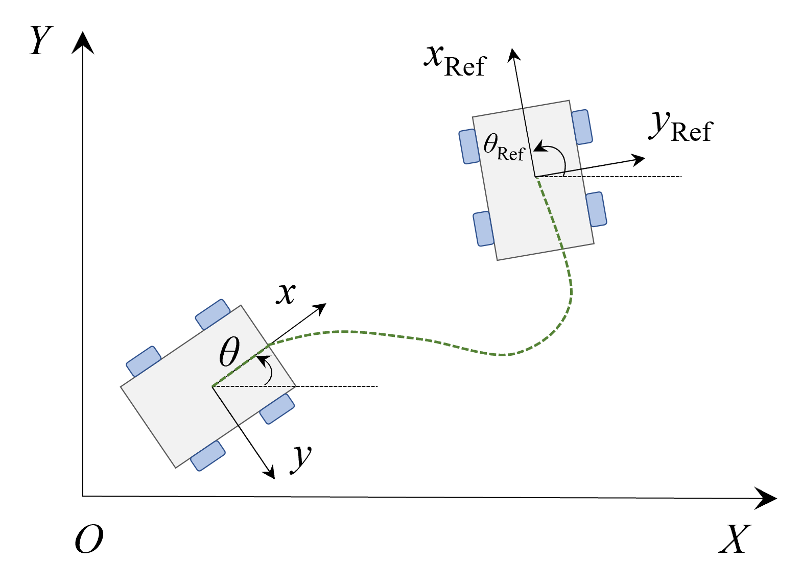
Figure 1: Nonholonomic mobile robot

The state and control signal vectors are defined as $\mathbf{x}=(x,y,\theta)^{T}$ and $\mathbf{u}=(v,\omega)^{T}$. In order to illustrate the control problems of the mobile robot, a reference robot with reference state vector $\mathbf{x}_{r}=(x_{r},y_{r},\theta_{r})^{T}$ and a reference control vector $\mathbf{u}_{r}=(v_{r},\omega_{r})^{T}$ is shown in Fig. 1. The reference robot has the same constraints as (1) and its kinematic model is written as:

$$\dot{\mathbf{x}}_{r}=\begin{bmatrix}\dot{x}_{r}\\ \dot{y}_{r}\\ \dot{\theta}_{r}\end{bmatrix}=\begin{bmatrix}v_{r}\cos(\theta_{r})\\ v_{r}\sin(\theta_{r})\\ \omega_{r}\end{bmatrix}=\begin{bmatrix}\cos(\theta_{r})&0\\ \sin(\theta_{r})&0\\ 0&1\end{bmatrix}\mathbf{u}_{r}$$ (2)

Two control problems are considered for the mobile robot. The point stabilization problem has a constant reference state vector $\mathbf{x}_{r}$, which is the target position, and a zero control vector $\mathbf{u}_{r}=(0,0)^{T}$. Meanwhile, the trajectory tracking problem contains time-varying state vector $\mathbf{x}_{r}$ and control vector $\mathbf{u}_{r}$, which depend on the chosen reference trajectory. In both cases, to control (1) to follow (2), an error state $\mathbf{x}_{e}$ can be defined as follows Y. J. Kanayama et al., (1990):

$${\mathbf{x}}_{e}=\begin{bmatrix}x_{e}\\ y_{e}\\ \theta_{e}\end{bmatrix}=\begin{bmatrix}\cos(\theta)&\sin(\theta)&0\\ -\sin(\theta)&\cos(\theta)&0\\ 0&0&1\end{bmatrix}\begin{bmatrix}x_{r}-x\\ y_{r}-y\\ \theta_{r}-\theta\end{bmatrix}$$ (3)

It can be easily seen that the two control objectives can be achieved by driving the state vector $\mathbf{x}_{e}$ to zero. The error dynamic model is obtained by differentiating (3) as:

$$\dot{\mathbf{x}}_{e}=\begin{bmatrix}\dot{x}_{e}\\ \dot{y}_{e}\\ \dot{\theta}_{e}\end{bmatrix}=\begin{bmatrix}\omega y_{e}-v+v_{r}\cos(\theta_{e})\\ -\omega x_{e}+v_{r}\sin(\theta_{e})\\ \omega_{r}-\omega\end{bmatrix}$$ (4)

Redefining the control signals

$$\mathbf{u}_{e}=\begin{bmatrix}u_{e1}\\ u_{e2}\end{bmatrix}=\begin{bmatrix}v_{r}\cos(\theta_{e})-v\\ \omega_{r}-\omega\end{bmatrix}$$ (5)

A linearized version of the error model (4) has the following form

$$\Delta\dot{\mathbf{x}}_{e}=\begin{bmatrix}x_{e}\\ y_{e}\\ \theta_{e}\end{bmatrix}=\begin{bmatrix}0&\omega_{r}&0\\ -\omega_{r}&0&v_{r}\\ 0&0&0\end{bmatrix}\Delta\mathbf{x}_{e}+\begin{bmatrix}1&0\\ 0&0\\ 0&1\end{bmatrix}\mathbf{u}_{e}$$ (6)

It can be easily checked that the controllability of model (6) for the stabilization problem is lost when $(\lim_{t\rightarrow\infty}(v_{r}(t)^{2}+\omega_{r}(t)^{2})=0)$. Independent controllers have been proposed for the two control problems. The switching between two independent controllers is needed when the tracking robot is required to stop. To avoid the switching, a single controller with simultaneous tracking and regulation capability is necessary.

3 NONLINEAR MODEL PREDICTIVE CONTROL DESIGN

A nonlinear nominal control system without considering any uncertainties, like (1), can be generally expressed as follows:

$$\dot{\mathbf{x}}(t)=f(\mathbf{x}(t),\mathbf{u}(t))$$ (7)

where $\mathbf{x}(t)\in R^{n}$ and $\mathbf{u}(t)\in R^{m}$ are the $n$ dimensional state and $m$ dimensional control vectors, respectively. To design NMPC for the mobile robot, the system dynamic (7) is discretized. The Runge-Kutta method (RK4) shows good approximate solutions of nonlinear ordinary differential equations for a larger sampling time ($T_{s}$). In this paper, the future states are approximated by RK4. The control task is to compute an admissible control input $\mathbf{u}(t)$ to drive the system (1) to move toward the equilibrium point by minimizing a given cost function as follows:

$$\begin{array}[]{l}J_{N}\left(\mathbf{x}_{e}\left(k\right),\mathbf{u}_{e}\left(k\right)\right)=g\left(\mathbf{x}_{e}\left(N\right)\right)\\ +\sum_{k=0}^{N-1}{\left(\mathbf{x}_{e}\left(k\right)^{T}Q\mathbf{x}_{e}\left(k\right)+\mathbf{u}_{e}\left(k\right)^{T}R\mathbf{u}_{e}\left(k\right)\right)}\end{array}$$ (8)

where $N$ is the prediction horizon. $Q=diag(q_{1},q_{2},q_{3})$ and $R=diag(r_{1},r_{2})$ are positive definite symmetric weight matrixes. $g$(.) is a positive definite terminal state penalty, which is added to guarantee the NMPC stability, M. R. Azizi et al., (2017). Therefore, the control problems of the mobile robot are formulated as the following optimal control problem (OCP):

$$\underset{\boldsymbol{u}}{\min}\,\,J_{N}\left(\mathbf{x}_{e}\left(k\right),\mathbf{u}_{e}\left(k\right)\right)$$ (9)

subject to

$$\mathbf{x}\left(k+1\right)=\mathbf{f}\left(\mathbf{x}\left(k\right),\mathbf{u}\left(k\right)\right),$$ (10a)

$$\mathbf{x}\left(\mathbf{x}_{0},0\right)=\mathbf{x}_{0},$$ (10b)

$$\mathbf{x}_{e}\left(N\right)\in\Omega,$$ (10c)

$$\mathbf{x}_{min}\leqslant\mathbf{x}\left(k\right)\leqslant\mathbf{x}_{max},\,\,\forall k\in\left[0,N\right],$$ (10d)

$$\mathbf{u}_{min}\leqslant\mathbf{u}\left(k\right)\leqslant\mathbf{u}_{max},\,\,\forall k\in\left[0,N-1\right],$$ (10e)

where $\Omega$ is a terminal-state region. The result of the above OCP is a sequence of $N$ input vectors as:

$$\mathbf{u}_{N}^{*}=\left[\mathbf{u}^{*}\left(k+1\right),\mathbf{u}^{*}\left(k+2\right),...,\mathbf{u}^{*}\left(k+N\right)\right]\in\mathbf{U}^{N}$$ (11)

which leads to the optimal value function $J_{N}^{*}$ and yields the following optimal states sequence:

$$\mathbf{x}_{N}^{*}=\left[\mathbf{x}^{*}\left(k+1\right),\mathbf{x}^{*}\left(k+2\right),...,\mathbf{x}^{*}\left(k+N\right)\right]\in\mathbf{X}^{N}$$ (12)

The control inputs are discretized using the zero-order hold (ZOH), meaning that the control signal is only updated every sampling time. Hence, the control feedback law at the time, $t$, is defined as the first element of the control sequence (11) as follows:

$$\begin{array}[]{l}\mathbf{u}\left(k+1\right)=\mathbf{u}^{*}\left(k+1\right)\\ \mathbf{u}_{k}\left(t\right)=\mathrm{ZOH}_{k}\left(t\right),t_{k}\leqslant t\leqslant t_{k+T_{s}}\\ \end{array}$$ (13)

which leads to the following closed-loop dynamics

$$\begin{array}[]{l}\mathbf{x}\left(\mathbf{x}_{0},k+1\right)=\mathbf{f}\left(\mathbf{x}\left(\mathbf{x}_{0},k\right),\mathbf{u}\left(k+1\right)\right)\\ \mathbf{x}\left(\mathbf{x}_{0},0\right)=\mathbf{x}_{0};\mathbf{u}_{k}\left(t\right)=\mathrm{ZOH}_{k}\left(t\right)\\ \end{array}$$ (14)

As shown in M. R. Azizi et al., (2017), system (7) is asymptotically stable if a terminal-state controller $\mathbf{u}(k+1)$ exists such that the following condition is satisfied:

$$g\left(\mathbf{f}\left(\mathbf{x}_{e},\mathbf{u}_{e}\right)\right)-g\left(\mathbf{x}_{e}\right)+\left(\mathbf{x}_{e}^{T}Q\mathbf{x}_{e}+\mathbf{u}_{e}^{T}R\mathbf{u}_{e}\right)\leqslant 0$$ (15)

In order to find the terminal-state region, a Lyapunov function for the terminal-state penalty is defined as follows:

$$g\left(\mathbf{x}_{e}\left(N\right)\right)=\mathbf{x}_{e}\left(N\right)^{T}P\mathbf{x}_{e}\left(N\right)$$ (16)

where $P=diag(p_{1},p_{2},p_{3})$ is a positive definite symmetric weight matrix.

It is assumed that for every pair $(\mathbf{x},\mathbf{x}_{r})$ there exists a control input $\mathbf{u}\in\mathbf{U}$ to move the states of the system (14) to a new state $\mathbf{x}(k+1)\in\mathbb{R}^{3}$ which is closer to $\mathbf{x}_{r}$

$$\varDelta=\left\|\mathbf{x}(k+1)-\mathbf{x}_{r}\right\|^{2}-\left\|\mathbf{x}(k)-\mathbf{x}_{r}\right\|^{2}<0$$ (17)

Regarding the positive diagonal matrices as, $R=diag(\beta,\beta)$ and $P=diag(\alpha,\alpha,\alpha)$, the inquality condition (15) is rewritten as:

$$\begin{array}[]{l}\alpha\left(\left\|\mathbf{x}\left(k+1\right)-\mathbf{x}_{r}\right\|^{2}\right)-\alpha\left(\left\|\mathbf{x}\left(k\right)-\mathbf{x}_{r}\right\|^{2}\right)\\ +\left(\left\|\mathbf{x}\left(k\right)-\mathbf{x}_{r}\right\|^{2}\right)+\beta\left(\left\|\mathbf{u}\left(k\right)-\mathbf{u}_{r}\right\|^{2}\right)\leqslant 0\end{array}$$ (18)

Considering the assumption in (17) and the definition of the control input constraint set

$$\begin{array}[]{c}\alpha\cdot\varDelta+\left(\left\|\mathbf{x}\left(k\right)-\mathbf{x}_{r}\right\|^{2}\right)+\beta\left(\left\|\mathbf{u}\left(k\right)-\mathbf{u}_{r}\right\|^{2}\right)\\ \leqslant\alpha\cdot\varDelta+\left(\left\|\mathbf{x}\left(k\right)-\mathbf{x}_{r}\right\|^{2}\right)+2\beta\mathbf{u}_{max}^{2}\leqslant 0\end{array}$$ (19)

Therefore, by choosing $\alpha\geqslant\frac{\left\|\mathbf{x}\left(k\right)-\mathbf{x}_{r}\right\|^{2}+2\beta\mathbf{u}_{max}^{2}}{\left|\varDelta\right|}$ the inequality (15) is satisfied and the terminal cost $g(.)$ is a control Lyapunov function. However, precomputation of $\mathbf{x}(k+1)$ and $\varDelta$ in each time step is not possible. Consequently, $\alpha$ should be chosen sufficiently large to satisfy the inequality (18) over the whole of the state space except a small neighborhood of the desired state.

4 OBSTACLE AVOIDANCE USING CONTROL BARRIER FUNCTION

The CBF is utilized in this section to derive a safety constraint for the nonlinear dynamic system (7), the objective is to find the optimal control signal such that the system position states always lie in a defined safe set $\mathscr{Z}\in R^{2}$. That is $\mathscr{Z}$ is forward invariant, i.e. if $\mathbf{x}\left(0\right)=\mathbf{x}_{0}\in\mathscr{Z}$ then $\mathbf{x}=\mathbf{x}\left(t\right)\in\mathscr{Z},\forall t$. The set $\mathscr{Z}$ is defined as:

$$\mathscr{Z}=\left\{\mathbf{x}\in D\subset\mathbb{R}^{2}|h\left(\mathbf{x}\right)\geqslant 0\right\},$$ (20)

$$\partial\mathscr{Z}=\left\{\mathbf{x}\in D\subset\mathbb{R}^{2}|h\left(\mathbf{x}\right)=0\right\},$$ (21)

$$\mathrm{Int}\left(\mathscr{Z}\right)=\left\{\mathbf{x}\in D\subset\mathbb{R}^{2}|h\left(\mathbf{x}\right)>0\right\},$$ (22)

Let $\mathscr{Z}$ be the superlevel set of a continuously differentiable function $h:\mathbb{R}^{2}\rightarrow\mathbb{R}$, then $h$ is a control barrier function (CBF) if there exists an extended class $\mathcal{K}_{\infty}$ function $\gamma$ such that for the control system (7)

$$\underset{\mathbf{u}\in\mathbf{U}}{\mathrm{sup}}\left[L_{f}h\left(\mathbf{x}\right)+L_{g}h\left(\mathbf{x}\right)\mathbf{u}\right]\geqslant-\gamma h\left(\mathbf{x}\right),\gamma\in\mathcal{K}_{\infty}$$ (23)

for all $\mathbf{x}\in D$. We can consider the set consisting of all control values at a point $\mathbf{x}\in D$ that render $\mathscr{Z}$ safe:

$$K_{cbf}\left(\mathbf{x}\right)=\left\{\mathbf{u}\in\mathbf{U}\,\,:L_{f}h\left(\mathbf{x}\right)+L_{g}h\left(\mathbf{x}\right)\mathbf{u}-\gamma h\left(\mathbf{x}\right)\geqslant 0\right\}$$ (24)

According to A. D. Ames et al., (2019), if $h$ is a control barrier function on $D$ and $\frac{\partial h}{\partial\mathbf{x}}\left(x\right)\neq 0$ for all $\mathbf{x}\in\partial\mathscr{Z}$, then any control signal $\mathbf{u}\in K_{cbf}\left(\mathbf{x}\right)$ for the system (7) render the set $\mathscr{Z}$ safe. Additionally, the set $\mathscr{Z}$ is asymptotically stable in $D$.

We consider rigid body obstacles and model them as the union of circles with centroids ($x_{ob,i}\left(t\right),y_{ob,i}\left(t\right)$) and fixed radius $r_{ob,i}$. Similarly, a circle defines a safe space of the robot by its center and a radius $r_{robot}$. We denote the $i$-th safety set as

$$\mathscr{Z}_{i}=\left\{\mathbf{x}\in\mathcal{X}\subset\mathbb{R}^{2}:h_{i}\left(\mathbf{x}\right)\geqslant 0\right\}$$ (25)

where

$$\begin{array}[]{l}h_{i}\left(\mathbf{x}\right)=\left(x\left(t\right)-x_{ob,i}\left(t\right)\right)^{2}+\left(y\left(t\right)-y_{ob,i}\left(t\right)\right)^{2}\\ -\left(r_{robot}+r_{ob,i}\right)^{2}\end{array}$$ (26)

In order to incorporate the CBF constraint inside the discrete-time NMPC in (10a). The condition in (23) is extended to the discrete-time domain which is shown as follows:

$$h_{i}\left(\mathbf{x}_{k+1}\right)-h_{i}\left(\mathbf{x}_{k}\right)\geqslant-\gamma h_{i}\left(\mathbf{x}_{k}\right),0<\gamma<1$$ (27)

Note that in (27) we defined $\gamma$ as a scalar instead of a $\mathcal{K}_{\infty}$ function as in (23) to simplify the notations for further discussions.

Assuming that the robot can detect the position and the size of the obstacles by its sensors. We consider the problem of regulating to the target state for the discrete-time system (10a) while ensuring safety in the context of set invariance. The proposed control logic NMPC-CBF solves the following constrained finite-time optimal control problem with horizon $N$ at each time step $T_{s}$

$$\underset{\boldsymbol{u}}{\min}\,\,J_{N}\left(\mathbf{x}_{e}\left(k\right),\mathbf{u}_{e}\left(k\right)\right)$$ (28)

subject to

$$\mathbf{x}(k+1)=\mathbf{f}(\mathbf{x}(k),\mathbf{u}(k)),$$ (29a)

$$\mathbf{x}(\mathbf{x}_{0},0)=\mathbf{x}_{0},$$ (29b)

$$\mathbf{x}_{e}(N)\in\Omega,$$ (29c)

$$\mathbf{x}_{min}\leqslant\mathbf{x}(k)\leqslant\mathbf{x}_{max},\,\,\forall k\in[0,N],$$ (29d)

$$\mathbf{u}_{min}\leqslant\mathbf{u}(k)\leqslant\mathbf{u}_{max},\,\,\forall k\in[0,N-1],$$ (29e)

$$\varDelta h_{i}(\mathbf{x}_{k+1},\mathbf{u}_{k+1})\geqslant-\gamma h_{i}(\mathbf{x}_{k}),\,\,\forall k\in[0,N-1],$$ (29f)

Several methods of avoiding obstacles were summarized in V. A. Bhavesh, (2015). Another suitable obstacle avoidance algorithm for NMPC is the Bug-Type (BT) algorithm. In BT algorithms, the robot moves on the shortest path from its initial position toward the goal position until it encounters an obstacle. The algorithm forces the robot to move tangentially around the surface of the obstacle and then return to its original path after completely dodging the obstacle. The formulation of BT is shown as follows:

$$\begin{array}[]{l}l_{i}\left(\mathbf{x}\right)=\sqrt{\left(x(t)-x_{ob,i}(t)\right)^{2}+\left(y(t)-y_{ob,i}(t)\right)^{2}}\\ -\left(r_{robot}+r_{ob,i}\right)\geqslant 0\\ \end{array}$$ (30)

This study formulates another NMPC with the BT constraints by replacing (29f) with (31) to compare the performance of two obstacle avoidance algorithms.

$$l_{i}\left(\mathbf{x}_{k+1}\right)\geqslant 0,\,\,\forall k\in\left[0,N-1\right]$$ (31)

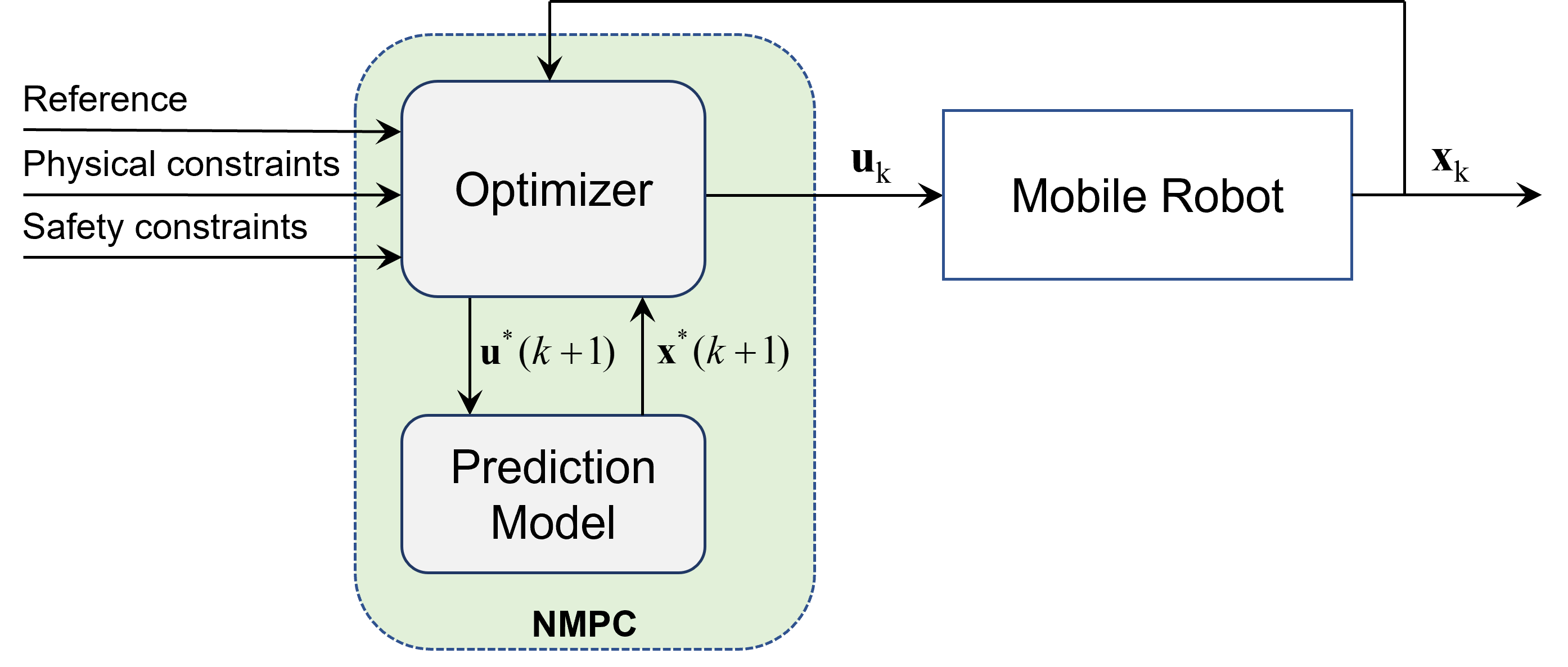
Figure 2: NMPC diagram

In this work, the NMPC algorithm is implemented by Casadi tool. The multiple-shooting approach was utilized to derive a nonlinear programming problem from the optimal control problem in (28) and (29). The NMPC block diagram overview is presented in Fig. 2. The feedback system states, the reference position, and the obstacle parameters are fed to the controller at each sampling instant for re-computation of the new optimal control strategy.

5 SIMULATIONS

Having presented the NMPC-CBF control design, we now numerically validate by two examples of point stabilization and trajectory tracking with static and dynamic obstacles.

5.1 CBF comparison with different values of $\gamma$

Consider the problem of regulating to a target state for the discrete-time system (29) while ensuring safety in the context of set invariance. The robot starts from an initial pose $\mathbf{x}_{0}=\left[x=0m,y=0m,\theta=0rad\right]^{T}$ and controlled to reach a target pose $\mathbf{x}_{r}=\left[2.5m,4m,-0.5rad\right]^{T}$ encountering five static obstacles at $(0.5m,1.5m)$, $(2.5m,2m)$, $(1m,4m)$, $(2m,3.5m)$, and $(3m,3.5m)$. The diameter of each obstacle is $1.4m$, $0.9m$, $0.7m$, $0.6m$, and $0.3m$ while the radius of the robot is $0.15m$. The sampling time is chosen to be $T_{s}=0.1s$ and a prediction horizon $N=10$ was selected leading to prediction horizon time $T=1s$. The robot’s actuator saturation limits are selected arbitrarily such that the linear velocity $v$ ranges are $\pm 0.6m/s$ and the angular velocity $\omega$ ranges are $\pm 0.78m/s$. The control parameters are chosen as: $q_{1}=5,q_{2}=10,q_{3}=0.7,r_{1}=5,r_{2}=0.1,P=100Q$.

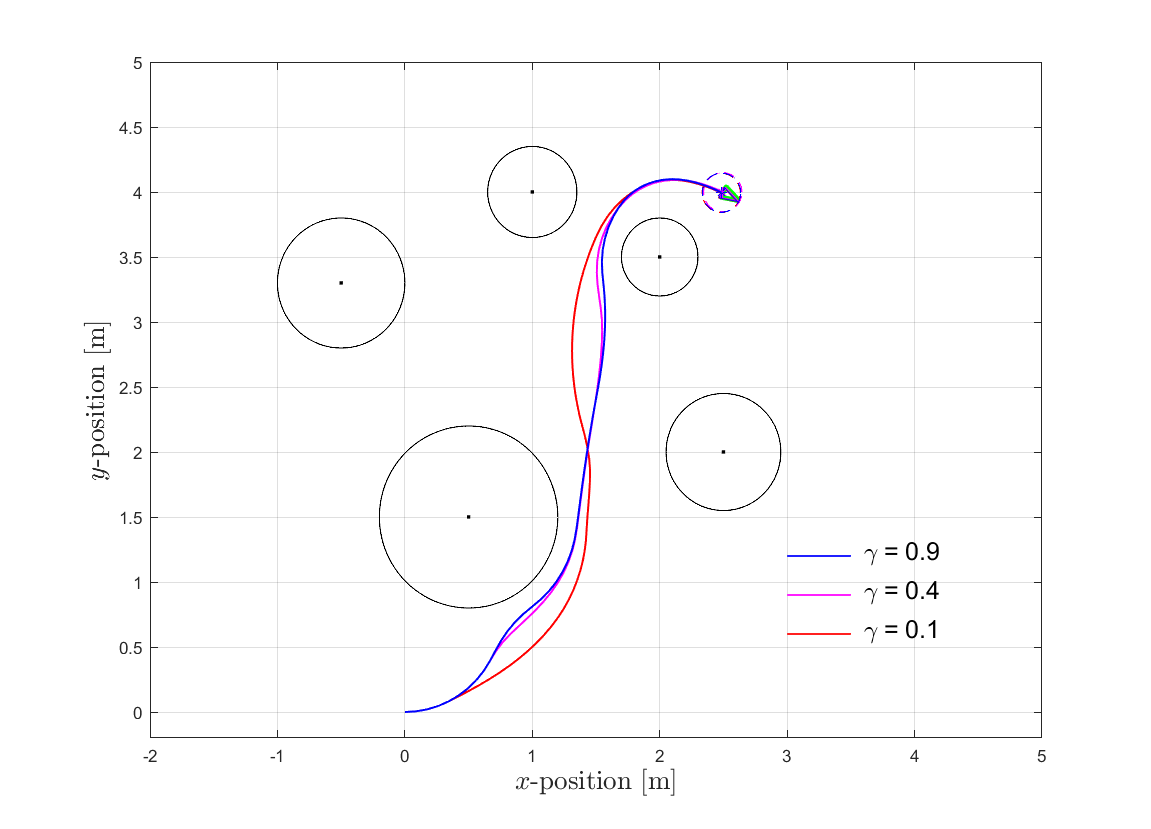
Figure 3: Robot avoids obstacles using $N=10$ and different $\gamma$ values

We illustrate the robot’s trajectory in different colors with three choices of $\gamma$ in Fig. 3. The obstacles are represented by a black circle. The robot with $\gamma=0.9$ does not start to avoid the obstacles until it is close to them. Meanwhile, a controller with a smaller $\gamma$ can drive the system to avoid obstacles earlier. By choosing an appropriate value of $\gamma$, the safety constraints can confine the robot’s movement to make the robot take actions even far away from obstacles. This advantage of CBF can help NMPC guarantees a safe trajectory with less horizon, which reduces the computational burden of NMPC. This will be emphasized in a comparison with NMPC-BT in the next simulation.

5.2 Comparison of NMPC-CBF and NMPC-BT

An NMPC-BT controller is developed based on (28) and (29). The NMPC-BT uses the same control parameters as NMPC-CBF except for the CBF constraints (29f), which is replaced by BT constraints (31). Point stabilization results are presented in Fig. 4 with the number of prediction horizons reduced to $N=5$. As can be seen in subplot (a) of Fig. 4, the CBF with $\gamma=0.3$ can stabilize the robot to the desired pose with a smooth obstacle-free trajectory. Meanwhile, the robot with the BT algorithm is stuck between two obstacles and cannot reach the goal position in the limited simulation time. Because the BT robot only has noticeable obstacle avoidance behavior when it is close to obstacles and the prediction horizon is too short in this case.

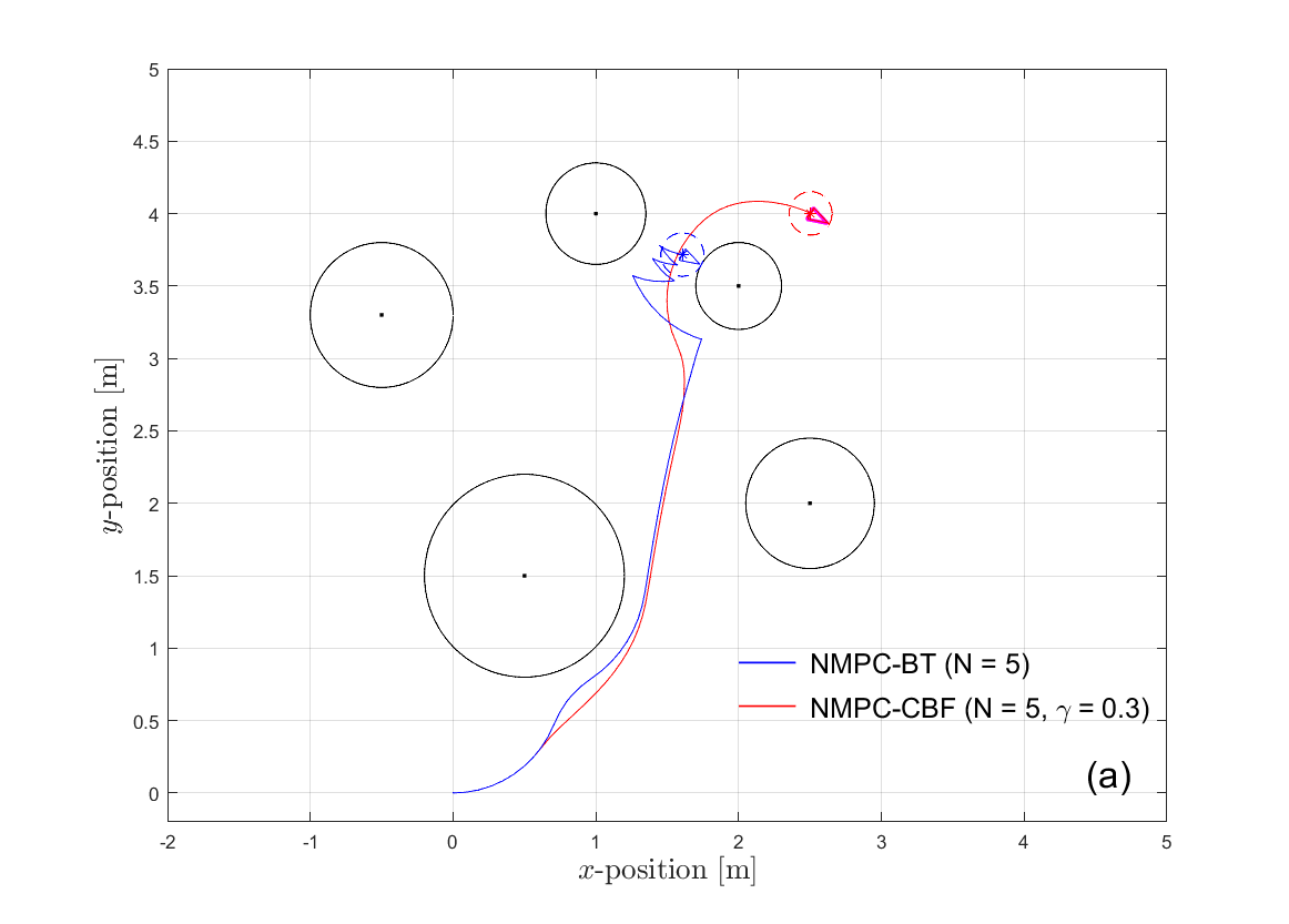
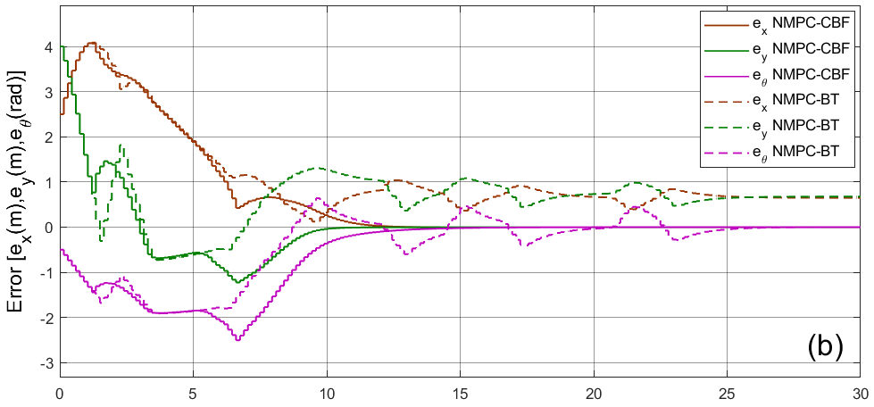
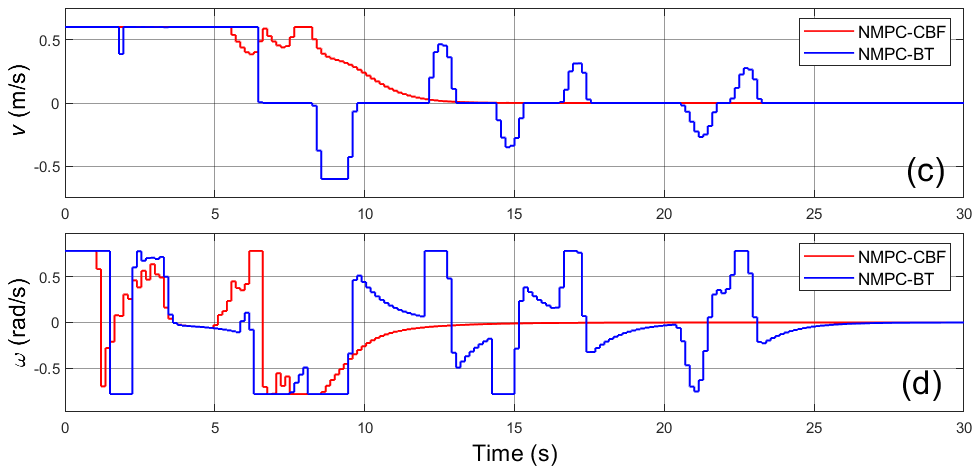
Figure 4: Robot avoids obstacles using $N=5$ and $\gamma=0.3$. (a) Trajectories; (b) Error state vector; (c) Linear speed; (d) Angular speed

5.3 Trajectory tracking in dynamic environment

In the second simulation, trajectory tracking tasks are conducted, where the reference trajectory follows a circular path defined as $[x_{r}(t)=0.7*cos(0.03t),\,\,y_{r}(t)=0.7*sin(0.03t)]^{T}$. The controller saturation limits in this case are $[-1,\,\,-0.8]^{T}\leqslant[v,\,\,\omega]^{T}\leqslant[1,\,\,0.8]^{T}$. Fig. 5 presents the circular path tracing of the robot for different cases. Due to the absence of obstacles, the tracking trajectory of NMPC-CBF with $N=5,\gamma=0.2$ quickly converges to the reference circle in Fig. 5(a). However, in a more complex scenario, we place three static obstacles across the reference path at $(2m,1m)$, $(0m,4.7m)$, and $(-2.3m,1.5m)$ with $r=0.4m$, $r=0.6m$, and $r=0.4m$, respectively. Besides, moving obstacles at different speeds are also considered in the simulation. The initial pose and the speed of moving obstacles are given as $(-8m,10m,-0.78rad;0.63m/s)$, $(0.5m,1.5m,-1rad;0.4m/s)$, $(-0.7m,-5m,1.5rad;0.31m/s)$, and $(5.5m,3m,-3.14rad;0.34m/s)$. As shown in Fig. 5 (b) and (c), two controllers can guarantee good tracking performance and safety with a long prediction horizon, $N=10$. Nonetheless, to examine the effects of CBF, we present the result of the same problem in Fig. 5 (b) and (c) which uses a shorter prediction horizon. It can be seen that CBF can still show a better tracking performance over BT despite using a prediction horizon of $N=5$. Fig. 6 illustrates the two controller’s performances of the simulation in Fig. 5(d). Fig. 6(a) shows the evolution of the error state vector $\mathbf{x}_{e}$ over the experiments running time for all cases. Several large overshoots in the error state of NMPC-BT are observed because the robot is stuck at the obstacles. The control signals stay within their limitations in Fig. 6 (b) and (c). The average computational times of the trajectory tracking simulation in Fig. 5(d) are shown in table 1. By using CBF, we can reduce the length of the parameter vector of the optimization problem from $(n_{\mathbf{x}}\times n_{\mathbf{u}}\times N)$ = 60 to 30 ($50\%$), which leads to a lower execution time per time step from 10.9$ms$ to 9.1$ms$ ($16.5\%$).

Table 1: Averaged computational time (in milliseconds)

	$N=5$	$N=10$
CBF without obstacle	7.5	8.5
CBF with obstacles	9.1	10.9
BT with obstacles	9.3	10.8

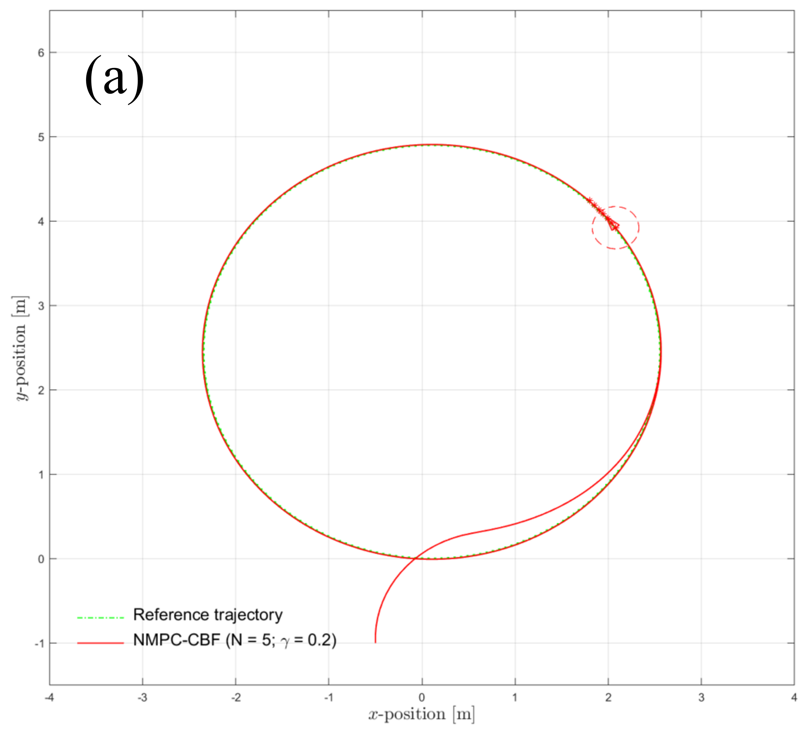
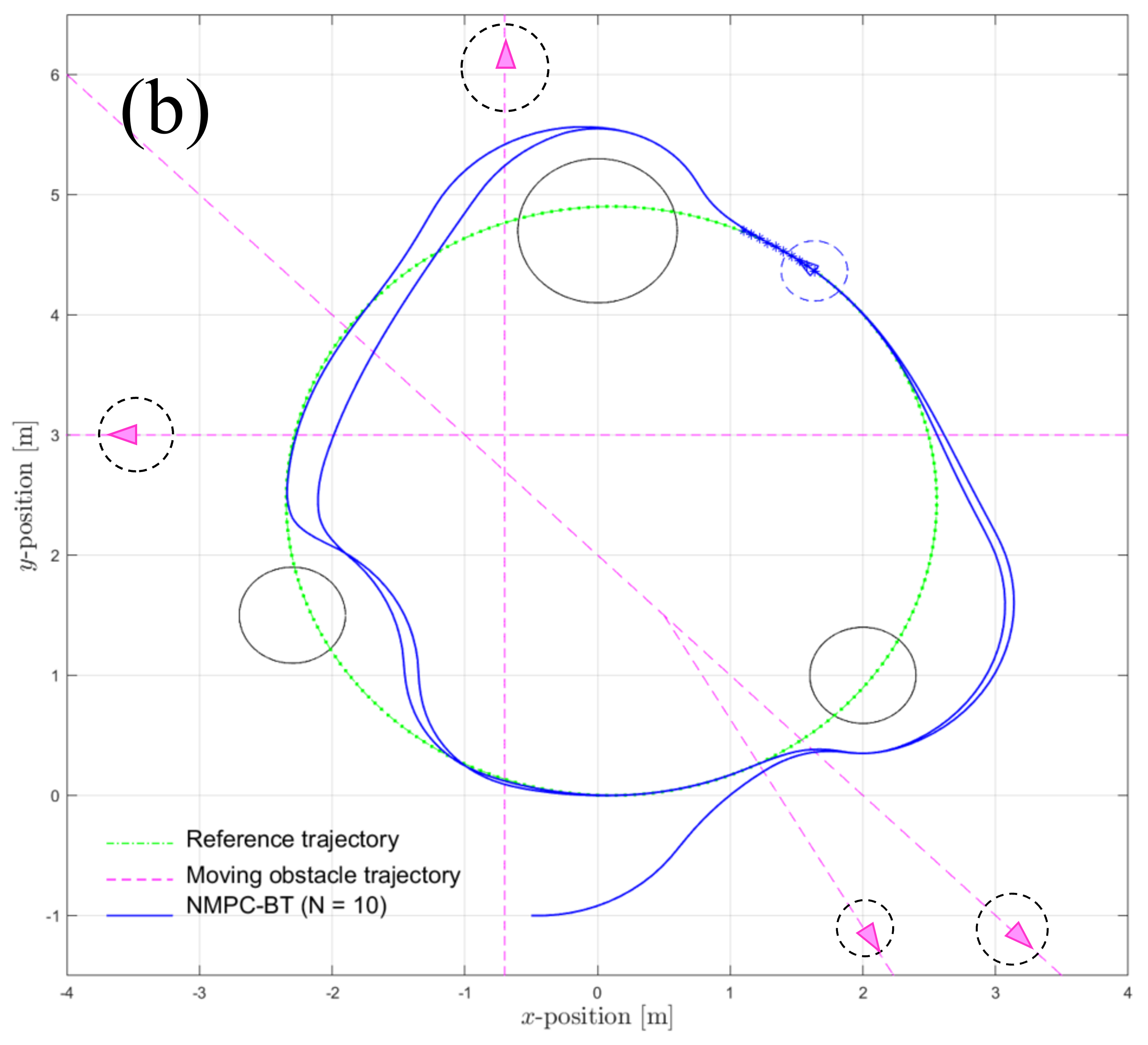
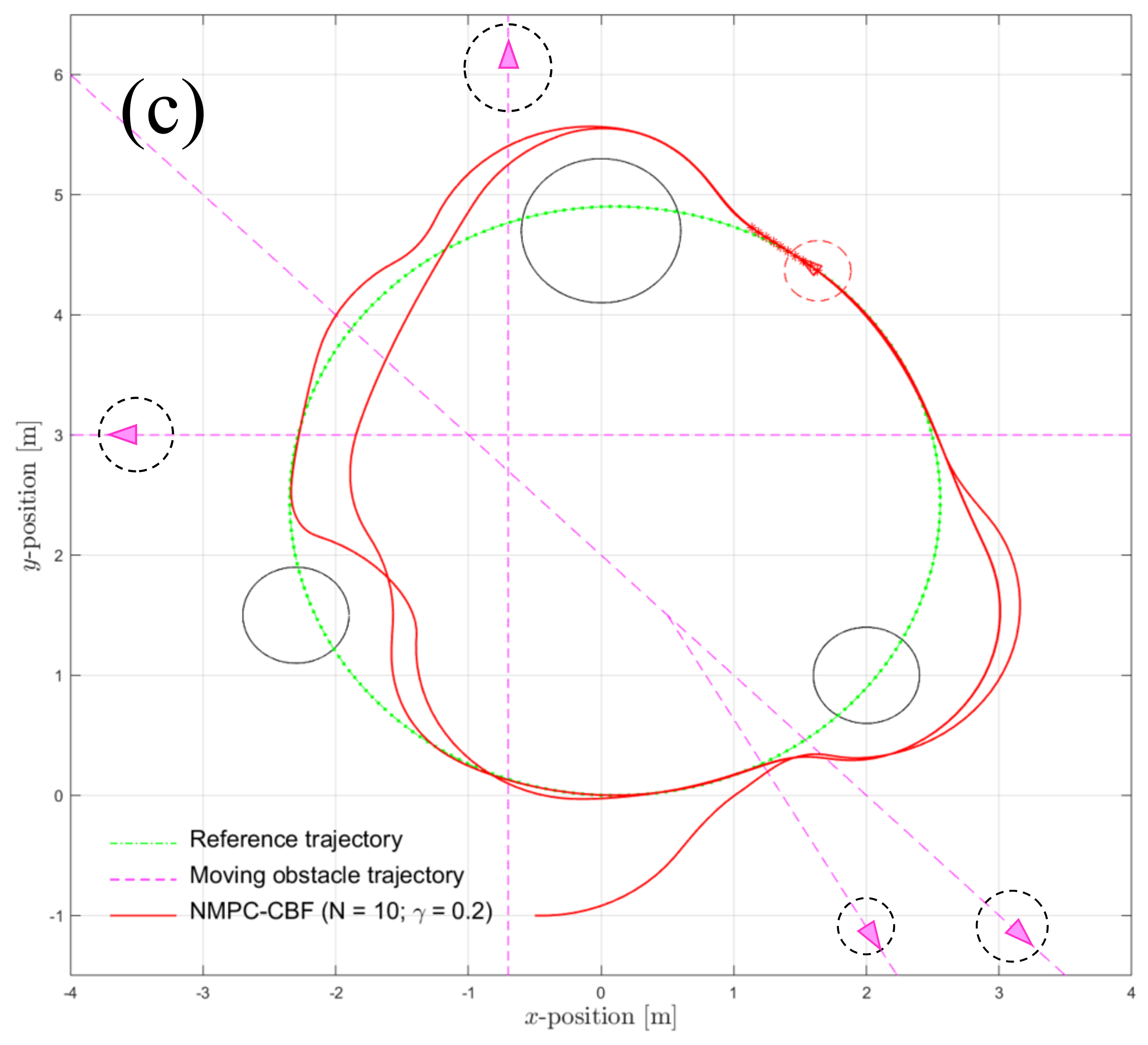
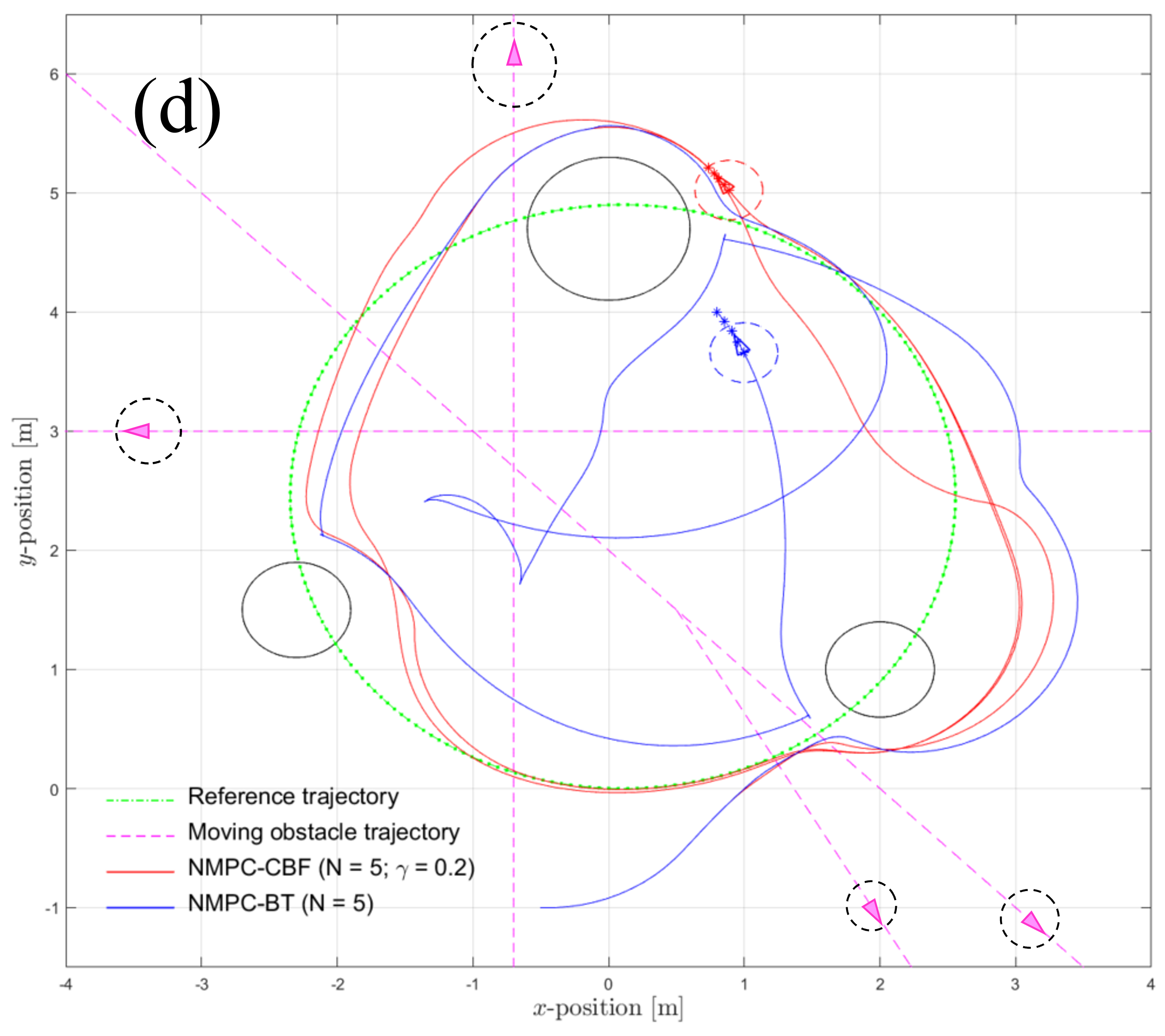
Figure 5: Trajectory tracking results. Detail of all simulations can be seen in this video:
https://youtu.be/My3hUBOSEyI

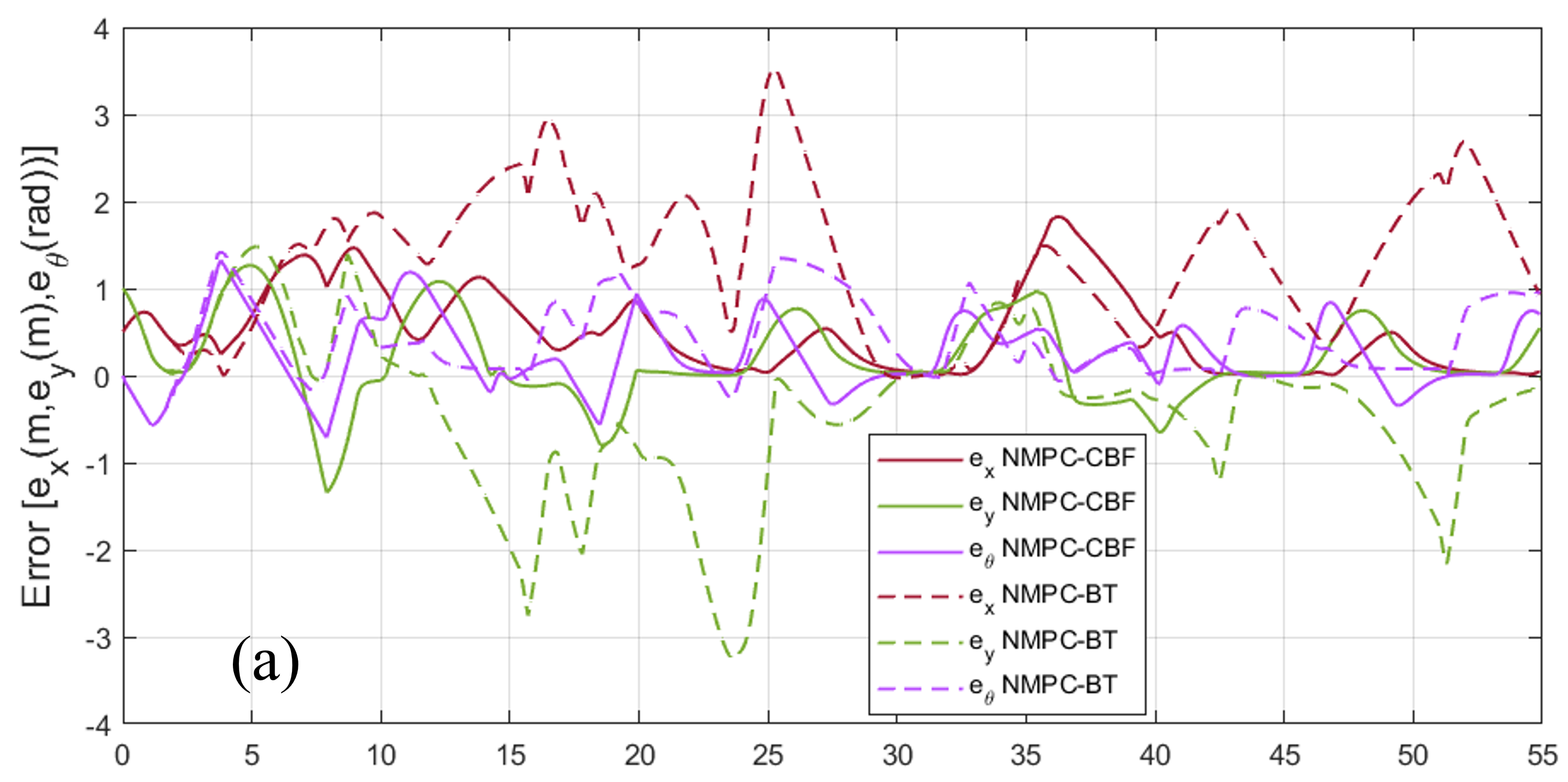
Figure 6: Trajectory tracking performance with obstacles using $N=5$ and $\gamma=0.3$. (a) Error state vector; (b) Linear speed; (c) Angular speed

6 Conclusion

In this paper, we have presented the formulation for a safety-critical model predictive control scheme that can incorporate either the Bug-Type algorithm or control barrier function to provide safety constraints. The two controller schemes are also simulated to achieve two common control objectives for mobile robots, i.e. point stabilization and trajectory tracking in different scenarios. The performances of NMPC-CBF and NMPC-BT are then analyzed, showing that dynamic obstacle avoidance can be achieved by both but that the CBF scheme can operate successfully with a smaller prediction horizon which can make it more computationally efficient for the purposes of practical implementation.

References

- S. G. Tzafestas, (2014) Spyros G. Tzafestas, Introduction to Mobile Robot Control, Elsevier, pp. 1-29, 2014.
- F. Xie et al., (2008) F. Xie and R. Fierro, First-state contractive model predictive control of nonholonomic mobile robots, Proceedings of the American Control Conference, pp. 3494-3499, 2008.
- G. Klanar et al., (2008) G. Klanar and I. . krjanc, Tracking-error model-based predictive control for mobile robots in real time, Robotics and Autonomous Systems, vol. 55, no. 6, pp. 460-469, 2007.
- T. P. Nascimento et al., (2018) T. P. Nascimento, C. E. T. Dórea, and L. M. G. Gonçalves, Nonholonomic mobile robots’ trajectory tracking model predictive control: A survey, Robotica, vol. 36, no. 5, pp. 676–696, Jan. 2018.
- R. W. Brockett et al., (1983) R. W. Brockett, R. S. Millman, and H. J. Sussmann, Differential Geometric Control Theory, Boston, MA, USA: Birkhhauser, 1983.
- B. d’Andrea-Novel et al., (1995) B. d’Andrea-Novel, G. Campion, and G. Bastin, Control of nonholonomic wheeled mobile robots by state feedback linearization, Int. J. Robot. Res, vol. 14, no. 6, pp. 543–559, 1995.
- U. Kumar et al., (2008) U. Kumar and N. Sukavanam, Backstepping based trajectory tracking control of a four wheeled mobile robot, International Journal of Advanced Robotic Systems, vol. 5, no. 4, pp. 403 - 410, 2008.
- Z. P. Jinag et al., (1997) Z. P. Jinag and H. Nijmeijer, Tracking control of mobile robots: A case study in backstepping, Automatica, vol. 33, pp. 1393–1399, 1997.
- D. Chwa, (2004) D. Chwa, Sliding-mode tracking control of nonholonomic wheeled mobile robots in polar coordinates, IEEE Transactions on Control Systems Technology, vol. 12, no. 4, pp. 637-644, 2004.
- C. de Wit et al., (1992) . de Wit and O. J. Sørdalen, Exponential stabilization of mobile robots with nonholonomic constraints, IEEE Trans. Autom. Control, vol. 37, no. 11, pp. 1791–1797, Nov. 1992.
- A. Tee et al., (1995) A. Teel, R. Murray, and C. Walsh, Nonholonomic control systems: From steering to stabilization with sinusoids, Int. J. Control, vol. 62, no. 4, pp. 849–870, 1995.
- W. E. Dixon et al., (2000) W. E. Dixon, D. M. Dawson, F. Zhang, and E. Zergeroglu, Global exponential tracking control of a mobile robot system via a PE condition, IEEE Transactions on Systems, Man, and Cybernetics-Part B: Cybernetics, vol. 30, no. 1, pp. 129–142, Feb. 2000.
- T. C. Lee et al., (2001) T. C. Lee, K. T. Sun, C. H. Lee, and C. C. Teng, Tracking control of unicycle-modeled mobile robots using s saturation feedback controller, IEEE Transactions on Control Systems Technology, vol. 9, no. 2, pp. 305–318, Mar. 2001.
- G. Oriolo et al., (2002) G. Oriolo, A. De Luca, and M. Vendittelli, WMR control via dynamic feedback linearization: Design, implementation, and experimental validation, IEEE Transactions on Control Systems Technology, vol.10, no. 6, pp. 835–852, 2002.
- M. W. Mehrez et al., (2015) Mohamed W. Mehrez, George K. I. Mann, and Raymond G. Gosine, Comparison of stabilizing nmpc designs for wheeled mobile robots: An experimental study, In 2015 Moratuwa Engineering Research Conference (MERCon), pages 130–135, 2015.
- A. D. Ames et al., (2014) A. D. Ames, K. Galloway, K. Sreenath, and J. W. Grizzle, Rapidly exponentially stabilizing control lyapunov functions and hybrid zero dynamics, IEEE Trans. on Automatic Control, vol. 59, pp. 876–891, Apr. 2014.
- M. Z. Romdlony et al., (2016) M. Z. Romdlony and B. Jayawardhana, Stabilization with guaranteed safety using control Lyapunov-Barrier Function, Automatica, vol. 66, pp. 39–47, Oct. 2016.
- M. Rauscher et al., (2016) M. Rauscher, M. Kimmel, and S. Hirche, Constrained robot control using control barrier functions, Proc. IEEE/RSJ Int. Conf. Intell. Robots Syst, vol. 66, pp. 279–285, Oct. 2016.
- W. S. Cortez et al., (2019) W. S. Cortez, D. Oetomo, C. Manzie, and P. Choong, Control barrier functions for mechanical systems: Theory and application to robotic grasping, IEEE Trans. Control Syst. Technol, vol. 29, no. 2, pp. 530–545, Mar. 2019.
- Q. Nguyen et al., (2019) Q. Nguyen and K. Sreenath, Exponential control barrier functions for enforcing high relative-degree safety-critical constraints, American Control Conference (ACC), pp. 322–328, July 2016.
- D. Gu et al., (2006) D. Gu and H. Hu, Receding horizon tracking control of wheeled mobile robots, Control Systems Technology, IEEE Transactions on, vol. 14, no. 4, pp. 743–749, 2006.
- Y. J. Kanayama et al., (1990) Y. J. Kanayama, Y. Kimura, F. Miyazaki, and T. Noguchi, A stable tracking control method for an autonomous mobile robot, Proc. IEEE Int. Conf. Robot. Autom., pp. 384-389, 1990.
- M. R. Azizi et al., (2017) Mahmood Reza Azizi, Jafar Keighobadi, Point stabilization of nonholonomic spherical mobile robot using nonlinear model predictive control, Robotics and Autonomous Systems, vol. 98, pp. 347-359, 2017.
- A. D. Ames et al., (2019) A. D. Ames, S. Coogan, M. Egerstedt, G. Notomista, K. Sreenath and P. Tabuada, Control Barrier Functions: Theory and Applications, 18th European Control Conference (ECC), pp. 3420-3431, 2019.
- V. A. Bhavesh, (2015) Vayeda Anshav Bhavesh, Comparison of various obstacle avoidance algorithms, International Journal of Engineering Research and Technology (IJERT), 2015.