Hierarchically Modular Dynamical Neural Network
Relaxing in a Warped Space:
Basic Model and its Characteristics

Abstract

We propose a hierarchically modular, dynamical neural network model whose architecture minimizes a specifically designed energy function and defines its temporal characteristics. The model has an internal and an external space that are connected with a layered “internetwork” that consists of a pair of forward and backward subnets composed of static neurons (with an instantaneous time-course). Dynamical neurons with large time constants in the internal space determine the overall time-course. The model offers a framework in which state variables in the network relax in a warped space, due to the cooperation between dynamic and static neurons. We assume that the system operates in either a learning or an association mode, depending on the presence or absence of feedback paths and input ports. In the learning mode, synaptic weights in the internetwork are modified by strong inputs corresponding to repetitive neuronal bursting, which represents sinusoidal or quasi-sinusoidal waves in the short-term average density of nerve impulses or in the membrane potential. A two-dimensional mapping relationship can be formed by employing signals with different frequencies based on the same mechanism as Lissajous curves. In the association mode, the speed of convergence to a goal point greatly varies with the mapping relationship of the previously trained internetwork, and owing to this property, the convergence trajectory in the two-dimensional model with the non-linear mapping internetwork cannot go straight but instead must curve. We further introduce a constrained association mode with a given target trajectory and elucidate that in the internal space, an output trajectory is generated, which is mapped from the external space according to the “inverse” of the mapping relationship of the forward subnet.

Keywords: hierarchical; modular; dynamical neural network; neuronal bursting; inverse mapping; Lissajous curves.

1 Introduction

One of the earliest models of neurons was proposed by McCulloch and Pitts [33]. In combination with Hebb’s insights into neuronal mechanisms of learning [18], their static neuron model was the basis of such well-known learning machines as the Perceptron, ADALINE, and the Learning Matrix [45][65][48]. The period from the late 1950s to the early 1960s is significant in the sense that neural network research started in earnest [4]. An important limitation that surfaced about a decade later is that the XOR problem cannot be learned in the original Perceptron architecture [36]. Consequently, a quiet period in neural network research followed, although multiple interesting ideas and models were proposed even during this era [2][3][39] [28][64][15]. In 1986, the generalized delta rule was presented with specific simulation examples as an advanced version of the original delta rule, allowing multi-layered networks with non-linear neurons to be trained [47][46], and this revitalized neural network research. During this period, expectations about a “neurocomputer” also arose [20]. Although neural network-based computation may have failed to reach the level of practical use that had been expected by some, the 1980s can be considered a crucial period because of the large number of novel frameworks proposed in this time [29][19].

In parallel with studies of artificial neural networks, attempts to understand the function of biological neural networks based on the identified circuitry of the brain have a long history. Following the pioneering studies of the visual system by Hubel and Wiesel [27], the Cognitron and Neocognitron were introduced as computational models with a highly hierachical structure [10][11][14]. Even though it currently remains unclear whether the gap between biological knowledge and artificial models is narrowing, interest in deeply hierarchical neural structures continues to grow, and research into how to train such layered networks has been receiving attention in recent years. The excellent performances obtained in image and voice recognition [21][22][31]  can be pointed out as the reason for this growing interest. Hierarchy and modularity in neural architecture appear to be significant organizing principles that may effectively and adequately reduce the informational dimension [42][17]. Based on mathematical analyses of human neuroimaging data, research into searching modular and/or hierarchical structures from the viewpoint of understanding their organizing principles has attracted increasing attention [34][40].

Research related to the dynamics of neurons and networks originated with the modeling of neural membranes and with the analysis of circuits based primarily on a comparatively small number of neurons. The first deep understanding of the biophysics of neuronal membranes came with a mathematical model of the squid giant axon proposed in 1952 [23]. The complexity of this model was reduced to the phenomena considered essential in a set of lower-dimensional models [8][38]. With regards to the circuit analysis, the dynamical characteristics of a neuron are generally accounted for, but in most cases, are simplified to their essentials. Circuits are typically constructed with inhibitory and excitatory connections, and occasionally gap junctions [41]; their dynamical behavior is examined in terms of the mean frequency fluctuation of nerve impulses, which can be further abstracted with respect to oscillation (limit cycles), chaos, etc. [37][1].  Such approaches allow us to simplify the network dynamics sufficiently to understand, for instance, the behavior of large networks whose dynamics are proposed to stay in or close to a critical state [35][44]. These issues are further discussed in terms of synaptic plasticity and neuronal adaptation that offer the fascinating power and capability of neural networks [59][58] [61][57][32]. Specifically, the importance and effectiveness of Central Pattern Generators (CPGs) based on relatively small networks with dynamical neurons is being recognized for controlling locomotive robots [50]. In studies on dynamical neurons, either a biologically identified network or a network supposedly constructed in a building block manner is often employed. After a new idea was proposed, where the superordinate concept called an energy function can be utilized for deriving a network architecture [24][25], a study of generic dynamical neural networks was conducted using large-scaled networks [6][60][57][51]. This framework’s proposal was indispensable as a factor to increase the expectations for the above-mentioned neurocomputer, particularly with regard to parallel computation.

One overarching theme of signaling routes in the brain and the nervous system is the bidirectionality in connectivity. Even if we focus on a local area, mutual communication exists between layers, modules, and/or sub-modules. One example of models with mutual connections between layers is described in a series of those called Adaptive Resonance Theory [16]. On a larger scale, reciprocal connections between layers are also essential for generating organism-wide functions, like selective attention [12]. Thus, understanding network architectures in which multiple layers are connected reciprocally and in a multiplexing manner is a matter of great interest.

Of particular interest are studies in which various approaches from different fields are associated with one another. For instance, learning mechanisms and activity dynamics have frequently been discussed separately: the first in the context of how synaptic plasticity and static mapping could be related, and the second in understanding how activity varies in a dynamical neural network with fixed synaptic connections. In this sense, a series of models with bidirectional connections named Bidirectional Associative Memories (BAM) was highly influential [30], and training algorithms called Back-Propagation Through Time and Real-Time Recurrent Learning, by which a dynamical mapping relationship can be acquired in a recurrent neural network, have great potential [66][67]. In addtion, it is important to model effects that can be produced by combining multiple types of neurons with different time constants [53][54][43]. To clarify the existence of higher mechanisms in the brain, multiple fundamental principles must be integrated for a more general framework. One challenge is understanding the behavior of a dynamical neural network in which the characteristics of various neurotransmitters are accurately reflected [7]. Even though constructing a model is difficult using only common knowledge, it might be reasonable to build a consistent hypothesis [13].

In this paper, we try to construct a model that combines multiple frameworks as cooperative dynamical responses by two types of neurons with different time constants, fluctuations of neuronal firing rates including bursting activity, as well as hierarchy and modularity in neural architecture, bidirectional (centripetal and centrifugal) paths, and mapping with generalization. We then propose a hierarchically modular neural network model that operates using cooperativity between dynamic and static neurons. This model is based on two previous studies. The first [52] uses an architecture in which dynamical neurons are sandwiched between two static layered neural networks with mutually inverse mapping relationships, and it includes local and global feedback loops. Its distinctive feature is that, in a computational task to be processed, each of the different constraints can be satisfied conveniently in a warped inner space or a linear outer space owing to a mapper with an inverse mapping relationship that is “explicitly” set. However, that model was derived according to a bottom-up design approach, and it lacked the theoretical grounding that we propose in the current study in terms of the temporal derivative of an energy function. The other study [56] is a predecessor of our model, but it was limited to a simple proposal that assumed only a linear mapper. Furthermore, its dynamical behavior including how to train the total network was not discussed.

In Section 2, we describe the model and its derivation process in detail. Following a clarification of the network architecture, we explain the two kinds of operating modes: learning and association. In Section 3, we investigate the learning mode, i.e., how a part of the whole network, in which synaptic plasticity is supposed, can be trained in collaboration with activity dynamics. Starting from simulation studies of a one-dimensional model with linear mapping, we refer to a model with non-linear mapping and then expand it into a two-dimensional model. In the following section, we examine, as an association mode, the dynamical behavior of the network trained in the previous section. In Section 5, on the basis of the simulation results in Sections 3 and 4, we discuss the relationship between the learning and association modes as well as experiments that precisely investigate network dynamics as a constrained association mode, in which a target trajectory (instead of a goal point) is applied to an input port of the model. This work is curiosity-driven fundamental research [9] and was not developed with a view on direct applicability for solving practical problems. We summarize our results and look toward future work in the last section.

2 Model

2.1 Basic Concept

The following is an example of a dynamical neural network equation:

$$-c_{i}\frac{dU_{i}}{dt}=\sum_{j}T_{ij}V_{j}-\sum_{k}S_{ik}Z_{k}-J_{i}+\frac{U_{i}}{r_{i}}~{}.$$ (1)

$U_{i}$ and $V_{i}$ are the inner state (membrane potential) of the $i$-th neuron and its output voltage (short-time average impulse density) respectively; both are time-varying functions that are related to each other with the following input-output function:

$$V_{i}=g(~{}U_{i}~{})~{}.$$ (2)

$T_{ij}$ means the fixed-valued conductance of a direct connection from the $j$-th dynamical neuron to the $i$-th one. $Z_{k}$ is the voltage (short-term average impulse density) of an input from the outside of the model that is added to a time-constant circuit composed of dynamical neurons after being converted from voltage to current by the conductance $S_{ik}$. $J_{i}$ is a bias current injected from the outside. $c_{i}$ and $r_{i}$ are the values of capacitance and resistance in the $i$-th dynamical neuron, which together determine its time constant. The changes of the sign of each term in Eq. (1) determine whether the dynamics is convergent or divergent; this issue has often been discussed in terms of the energy function stated below after the framework was first proposed by Hopfield.

Consider the following energy function:

$$E \stackrel{{\scriptstyle\triangle}}{{=}} \frac{1}{2}\sum_{i}V_{i}~{}(~{}\sum_{j}T_{ij}V_{j}~{})~{}-\sum_{i}V_{i}~{}(~{}\sum_{k}S_{ik}Z_{k}~{})$$ (3)

$$\hskip 14.22636pt-\sum_{i}V_{i}J_{i}~{}+\sum_{i}\frac{1}{r_{i}}\int_{0}^{V_{i}}g^{-1}(V)dV~{}.$$

Differentiating this energy function with respect to time, we get

$$\frac{dE}{dt}=\sum_{i}\frac{dV_{i}}{dt}\mbox{\LARGE[}\sum_{j}T_{ij}V_{j}-\sum_{k}S_{ik}Z_{k}-J_{i}+\frac{U_{i}}{r_{i}}\mbox{\LARGE]}~{}.$$ (4)

Since the terms in the brackets of the right-hand side of Eq. (4) are the same as the right-hand side of Eq. (1), we can substitute Eq. (1) for Eq. (4). If we employ, in the network described by Eq. (1), the following monotonically increasing function as $g(x)$ in Eq. (2)

$$g(x)~{}=~{}\alpha x~{}~{}~{}~{}~{}~{}~{}~{}~{}~{}(~{}\alpha>0~{}:~{}\mbox{Const.}~{})~{},$$ (5)

or

$$g(x)~{}=~{}\frac{1}{1+e^{-\alpha x}}~{}~{}~{}~{}~{}~{}~{}~{}~{}~{}(~{}\alpha>0~{}:~{}\mbox{Const.}~{})~{},$$ (6)

taking $g^{\prime}(~{}U_{i}~{})>0$ into consideration, application of the chain rule in Eq. (4) yields

$$\frac{dE}{dt} = -~{}\sum_{i}~{}c_{i}~{}\mbox{\Large(}\frac{dV_{i}}{dt}\mbox{\Large)}~{}\mbox{\Large(}\frac{dU_{i}}{dt}\mbox{\Large)}$$ (7)

$$= -~{}\sum_{i}~{}c_{i}~{}g^{\prime}(U_{i})~{}\mbox{\Large(}\frac{dU_{i}}{dt}\mbox{\Large)}^{2}~{}~{}\leq 0~{}.$$

We thus find that $dE/dt$ is non-positive, showing that the value of the energy function given by Eq. (3) always decreases toward a global or a local minimum. By defining a task to be processed, such as an associative memory or an optimization problem, in the form of an energy function like Eq. (3), various problem-solving methods based on the dynamical neural network given by Eqs. (1) and (6) have been developed previously [26][49]. It should be noted that dynamics described by Eq. (1) generally include both convergent ( $U_{i}\rightarrow a$ / $V_{i}\rightarrow b$ ) and divergent ( ( $U_{i}\rightarrow-\infty$ / $V_{i}\rightarrow 0$ ) or ( $U_{i}\rightarrow+\infty$ / $V_{i}\rightarrow 1$ ) ) behaviors, where $a$ and $b$ are finite constants.

We will use a superscript with the form of $<0>$ to the output of a dynamical neuron $V_{i}$ to specify that neurons exist in the $0$-th space (the internal space). In addition, we suppose that the variables $V^{<0>}_{i}$, $(i=0,1,2,...)$ are converted to the output ones $V^{<1>}_{i^{\prime}},~{}(~{}i^{\prime}=0,1,2,...~{})$ in the upper $1$-st space (the external space) based on the following function:

$$V^{<1>}_{i^{\prime}}=f^{<1>}_{i^{\prime}}(V^{<0>}_{0},V^{<0>}_{1},V^{<0>}_{2},...~{})~{}.$$ (8)

Using the converted variables $V^{<1>}_{i^{\prime}}$, we now re-define the total energy function given by Eq. (9) on the assumption that the direct fixed-valued connection $T^{<P>}_{ij}$, ( $P=0,1$ ) is symmetric:

$$E \stackrel{{\scriptstyle\triangle}}{{=}} \frac{1}{2}\sum_{i^{\prime}}V^{<1>}_{i^{\prime}}~{}(~{}\sum_{j}T^{<1>}_{i^{\prime}j}~{}V^{<1>}_{j}~{})~{}-~{}\sum_{i^{\prime}}V^{<1>}_{i^{\prime}}~{}(~{}\sum_{k}S^{<1>}_{i^{\prime}k}~{}Z^{<1>}_{k}~{})$$ (9)

$$+~{}\frac{1}{2}\sum_{i}V^{<0>}_{i}~{}(~{}\sum_{j}T^{<0>}_{ij}~{}V^{<0>}_{j}~{})~{}-~{}\sum_{i}V^{<0>}_{i}~{}(~{}\sum_{k}S^{<0>}_{ik}~{}Z^{<0>}_{k}~{})$$

$$+~{}\sum_{i}\frac{1}{r_{i}}\int_{0}^{V^{<0>}_{i}}g^{-1}(V)dV~{}.$$

Differentiating Eq. (9) with respect to time, we obtain

$$\frac{dE}{dt} = \sum_{i^{\prime}}\frac{dV^{<1>}_{i^{\prime}}}{dt}\mbox{\Large(}\sum_{j}T^{<1>}_{i^{\prime}j}V^{<1>}_{j}-\sum_{k}S^{<1>}_{i^{\prime}k}Z^{<1>}_{k}\mbox{\Large)}$$ (10)

$$+\sum_{i}\frac{dV^{<0>}_{i}}{dt}\mbox{\Large(}\sum_{j}T^{<0>}_{ij}V^{<0>}_{j}-\sum_{k}S^{<0>}_{ik}~{}Z^{<0>}_{k}+\frac{U_{i}}{r_{i}}\mbox{\Large)}~{}.$$

$dV^{<1>}_{i^{\prime}}/dt$ in Eq. (10) can be transformed as follows:

$$\frac{dV^{<1>}_{i^{\prime}}}{dt}~{}=~{}\sum_{i}\frac{\partial V^{<1>}_{i^{\prime}}}{\partial V^{<0>}_{i}}\frac{dV^{<0>}_{i}}{dt}~{}.$$ (11)

Substituting Eq. (11) for Eq. (10), we get

$$\frac{dE}{dt} = \sum_{i}\frac{dV^{<0>}_{i}}{dt}~{}\mbox{\LARGE[}~{}\sum_{i^{\prime}}\frac{\partial V^{<1>}_{i^{\prime}}}{\partial V^{<0>}_{i}}\mbox{\Large(}~{}\sum_{j}T^{<1>}_{i^{\prime}j}V^{<1>}_{j}~{}-~{}\sum_{k}S^{<1>}_{i^{\prime}k}Z^{<1>}_{k}~{}\mbox{\Large)}~{}$$ (12)

$$+\sum_{j}T^{<0>}_{ij}V^{<0>}_{j}-\sum_{k}S^{<0>}_{ik}~{}Z^{<0>}_{k}+\frac{U_{i}}{r_{i}}~{}\mbox{\LARGE]}~{}.$$

If we construct a dynamical neural network described by the following equation,

$$-~{}c_{i}\frac{dU_{i}}{dt} = \sum_{j}T^{<0>}_{ij}V^{<0>}_{j}-\sum_{k}S^{<0>}_{ik}~{}Z^{<0>}_{k}$$ (13)

$$+\sum_{i^{\prime}}~{}\frac{\partial V^{<1>}_{i^{\prime}}}{\partial V^{<0>}_{i}}~{}\mbox{\Large(}~{}\sum_{j}T^{<1>}_{i^{\prime}j}V^{<1>}_{j}~{}-\sum_{k}S^{<1>}_{i^{\prime}k}Z^{<1>}_{k}~{}\mbox{\Large)}+\frac{U_{i}}{r_{i}}~{},$$

it always holds that $dE/dt\leq 0$ in the same way as in Eq. (7), and therefore the value of the energy function defined by Eq. (9) monotonically decreases as time proceeds. Figure 1 shows the block diagram of the ladder-shaped network described by Eq. (13). The part surrounded by a gray dotted line corresponds to the network represented by Eq. (1). Here the conversion from $V^{<0>}_{i}$ to $V^{<1>}_{i^{\prime}}$ by Eq. (8) is called Mapper M, and the product-sum operation with $\partial V^{<1>}_{i^{\prime}}/\partial V^{<0>}_{i}$ is called Mapper N. The network has two kinds of feedback paths. One is in the internal space and is included in Eq. (1). The other is in the external space, and due to this feedback path by Mapper M, the connections $T^{<1>}_{i^{\prime}j}$, and Mapper N, the output signal in the internal space is returned again to the dynamical neurons in the internal space.

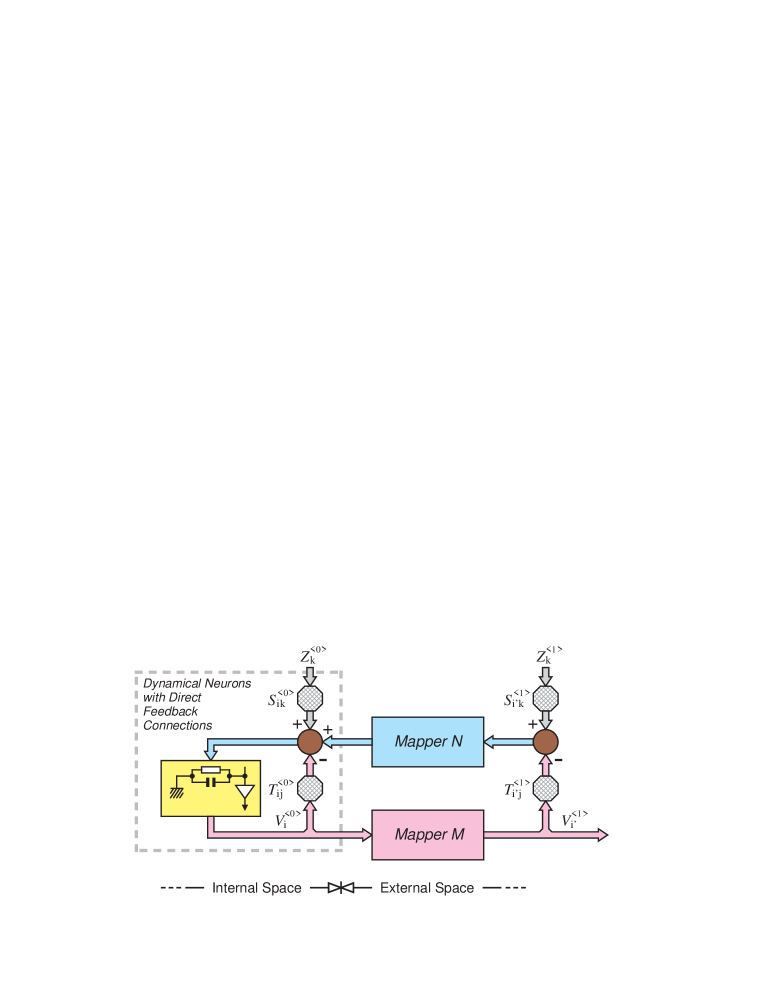
Figure 1: A block diagram of the network described by Eq. (13). Conversion from $V^{<0>}_{i}$ to $V^{<1>}_{i^{\prime}}$ is called Mapper M, and a product-sum operation with $\partial V^{<1>}_{i^{\prime}}/\partial V^{<0>}_{i}$ is called Mapper N. The network has two kinds of feedback paths. One is in the internal space and is included in Eq. (1). The other is via the external space; the output in the internal space is returned back to dynamical neurons in the internal space through Mapper M, the connections $T^{<1>}_{i^{\prime}j}$, and Mapper N. The network also has an input port in each space.

2.2 Static Neurons

In the previous subsection, we assumed that $V^{<0>}_{i}$ and $V^{<1>}_{i^{\prime}}$ were related to each other by Eq. (8). Now we use a layered neural network composed of neurons with a very small time constant that can be regarded as static. In the formulation, the layer number is assigned from $0$ to $L-1$, and the sum of the inputs applied to each neuron in the $l$-th layer and the neuronal output are $net^{<1><l>}_{i}$ and $O^{<1><l>}_{i}$. A modifiable connection from the $j$-th neuron in the $l$-th layer to the $i$-th neuron in the $(l+1)$-th layer is written as $W^{<1><l>}_{ij}$. We regard the output of a neuron in the layered network $O^{<1><L-1>}_{i}$ as the output signal in the external space $V^{<1>}_{i}$ and maintain consistency with Eq. (8). The first superscript with the brackets $<$ and $>$ in such variables as $O$, $net$, and $W$ is $<1>$, since it is the one that becomes necessary after establishing the external space. Note that we redundantly employ such indices as $i$, $j$, and $k$ without their maximum values to reduce the number of indices.

A neuron in the input layer of the layered network is assumed to have linear characteristics represented by Eq. (5), and we make the input layer a simple relaying function to send $V^{<0>}_{i}$ directly to the layered network. In general, we employ a non-linear neuron described by Eq. (6) in the hidden layers, and a linear or non-linear neuron in the output layer. For simplicity, we assume that each neuron shares linearity or non-linearity inside the corresponding layer, although each can have its own input-output characteristics. The relation between these variables is as follows:

$$V^{<1>}_{i} \stackrel{{\scriptstyle\triangle}}{{=}} O^{<1><L-1>}_{i}$$ (14)

$$O^{<1><l>}_{i} = g(~{}net^{<1><l>}_{i}~{})$$ (15)

$$\mbox{where~{}~{}~{}~{}~{}}net^{<1><l>}_{i}=\sum_{j}W^{<1><l-1>}_{ij}O^{<1><l-1>}_{j}~{}.$$

$$\hskip 71.13188pt(~{}l=L-1,L-2,...,2,1~{})$$

The following is the time derivative of Eq. (14):

$$\frac{dV^{<1>}_{i}}{dt} = g^{\prime}(~{}net^{<1><L-1>}_{i}~{})~{}\times~{}\mbox{\Large(}~{}\sum_{j}\frac{dW^{<1><L-2>}_{ij}}{dt}~{}O^{<1><L-2>}_{j}$$ (16)

$$\hskip 56.9055pt+\sum_{j}W^{<1><L-2>}_{ij}~{}\frac{dO^{<1><L-2>}_{j}}{dt}~{}\mbox{\Large)}~{}.$$

Let us define $H$ as the first term on the right-hand side of Eq. (10),

$$H \stackrel{{\scriptstyle\triangle}}{{=}} \sum_{i}\frac{dV^{<1>}_{i}}{dt}~{}\mbox{\Large(}~{}\sum_{j}T^{<1>}_{ij}V^{<1>}_{j}~{}-\sum_{k}S^{<1>}_{ik}Z^{<1>}_{k}~{}\mbox{\Large)}~{},$$ (17)

and substitute Eq. (16) for Eq. (17). Then, after some rearrangements, we obtain

$$H = \sum_{i}\sum_{j}\frac{dW^{<1><L-2>}_{ij}}{dt}~{}O^{<1><L-2>}_{j}~{}\delta^{<1><L-1>}_{i}$$ (18)

$$~{}+\sum_{j}\frac{dO^{<1><L-2>}_{j}}{dt}~{}\times~{}\mbox{\Large(}~{}\sum_{i}W^{<1><L-2>}_{ij}~{}\delta^{<1><L-1>}_{i}~{}\mbox{\Large)}~{}.$$

Introducing $\delta^{<1><L>}_{i}$ for convenience,

$$\delta^{<1><L>}_{i} \stackrel{{\scriptstyle\triangle}}{{=}} \sum_{j}T^{<1>}_{ij}V^{<1>}_{j}-\sum_{k}S^{<1>}_{ik}Z^{<1>}_{k}~{},$$ (19)

$\delta^{<1><L-1>}_{i}$ in Eq. (18) is written as follows:

$$\delta^{<1><L-1>}_{i} \stackrel{{\scriptstyle\triangle}}{{=}} g^{\prime}(~{}net^{<1><L-1>}_{i}~{})~{}\delta^{<1><L>}_{i}~{}.$$ (20)

The variable $\delta$ is also needed after the supposition of the external space, so the first superscript with $<$ and $>$ is assumed to be $<1>$. Further calculating $dO^{<1><L-2>}_{j}/dt$ in Eq. (18) based on Eq. (15) yields

$$H = \sum_{i}\sum_{j}\frac{dW^{<1><L-2>}_{ij}}{dt}~{}O^{<1><L-2>}_{j}~{}\delta^{<1><L-1>}_{i}$$ (21)

$$+~{}\sum_{j}\sum_{k}\frac{dW^{<1><L-3>}_{jk}}{dt}~{}O^{<1><L-3>}_{k}~{}\delta^{<1><L-2>}_{j}$$

$$+~{}\sum_{k}\frac{dO^{<1><L-3>}_{k}}{dt}~{}\times~{}\mbox{\Large(}~{}\sum_{j}W^{<1><L-3>}_{jk}~{}\delta^{<1><L-2>}_{j}~{}\mbox{\Large)}~{},$$

where

$$~{}\delta^{<1><L-2>}_{j} \stackrel{{\scriptstyle\triangle}}{{=}} g^{\prime}(~{}net^{<1><L-2>}_{j}~{})~{}\times~{}\mbox{\Large(}~{}\sum_{i}W^{<1><L-2>}_{ij}\delta^{<1><L-1>}_{i}~{}\mbox{\Large)}~{}.$$ (22)

We obtain the following equation after repeating these calculations from the output layer to the input layer:

$$H = \sum_{l=0}^{L-2}~{}\mbox{\LARGE[}~{}\sum_{i}\sum_{j}\frac{dW^{<1><l>}_{ij}}{dt}~{}\times~{}\mbox{\Large(}~{}O^{<1><l>}_{j}~{}\delta^{<1><l+1>}_{i}~{}\mbox{\Large)}~{}\mbox{\LARGE]}$$ (23)

$$~{}+\sum_{i}\frac{dO^{<1><0>}_{i}}{dt}~{}\mbox{\Large(}\sum_{j}W^{<1><0>}_{ji}~{}\delta^{<1><1>}_{j}\mbox{\Large)}~{}.$$

Here, $\delta$ is written with Eqs. (20) and (22) as follows:

$$\delta^{<1><l>}_{i} = g^{\prime}(~{}net^{<1><l>}_{i}~{})~{}\times~{}\mbox{\Large(}~{}\sum_{j}W^{<1><l>}_{ji}\delta^{<1><l+1>}_{j}~{}\mbox{\Large)}~{}.$$ (24)

$$\hskip 56.9055pt(~{}l=L-1,L-2,...,2,1~{})$$

As for the layered network, linear neurons are assumed in the input layer and simply relay the output of the dynamical neurons in the internal space to the upper layer; so we can put

$$O^{<1><0>}_{i}=V^{<0>}_{i}~{}.$$ (25)

Therefore, returning Eqs. (23) and (24) to Eq. (10) based on the above, we finally obtain

$$\frac{dE}{dt} = \sum_{i}\frac{dV^{<0>}_{i}}{dt}~{}\mbox{\Large(}~{}\sum_{j}T^{<0>}_{ij}V^{<0>}_{j}~{}-\sum_{k}S^{<0>}_{ik}Z^{<0>}_{k}~{}+\delta^{<1><0>}_{i}~{}+\frac{U_{i}}{r_{i}}~{}\mbox{\Large)}$$ (26)

$$+\sum_{l=0}^{L-2}~{}\mbox{\LARGE[}~{}\sum_{i}\sum_{j}\frac{dW^{<1><l>}_{ij}}{dt}~{}\times~{}\mbox{\Large(}~{}O^{<1><l>}_{j}~{}\delta^{<1><l+1>}_{i}~{}\mbox{\Large)}~{}\mbox{\LARGE]}~{},$$

where

$$\delta^{<1><0>}_{i}~{}\stackrel{{\scriptstyle\triangle}}{{=}}~{}\sum_{j}W^{<1><0>}_{ji}\delta^{<1><1>}_{j}~{}.$$ (27)

Here, constructing the network described by Eq. (28) and assuming that the connections in the layered neural network are modified according to Eq. (29),

$$-~{}c_{i}~{}\frac{dU_{i}}{dt} = \sum_{j}T^{<0>}_{ij}V^{<0>}_{j}-\sum_{k}S^{<0>}_{ik}Z^{<0>}_{k}+\delta^{<1><0>}_{i}+\frac{U_{i}}{r_{i}}~{},$$ (28)

$$-\eta^{<1><l>}_{ij}\frac{dW^{<1><l>}_{ij}}{dt} = O^{<1><l>}_{j}~{}\delta^{<1><l+1>}_{i}~{},$$

$$\hskip 28.45274pt(~{}l=L-2,L-3,...,1,0~{})$$

$dE/dt\leq 0$ always holds in the same way as in Eq. (7), and therefore the value of the energy function defined by Eq. (9) also monotonically decreases as time proceeds. $\eta^{<1><l>}_{ij}$ is a positive constant determining the learning speed. $\delta$ is given by Eqs. (19), (24), and (27), and $\delta^{<1><0>}_{i}$ in Eq. (27) can be calculated from $\delta^{<1><L>}_{i}$ according to Eqs. (19) and (24).

Expressing the computational process of $\delta$ explicitely as network architecture, the total network described by Eqs. (28) and (29) is illustrated as a block diagram in Fig. 2. Obviously, by comparison with Fig. 1, Mapper M and Mapper N in Fig. 1 are replaced by two layered networks that are complementary to each other. In the following sections, we call such a pair of layered networks Internetwork in the sense that it connects two spaces, and we name these two layered networks Forward Subnet and Backward Subnet respectively. In Fig. 2, we also call Internetwork’s left part the internal space and its right part the external space.

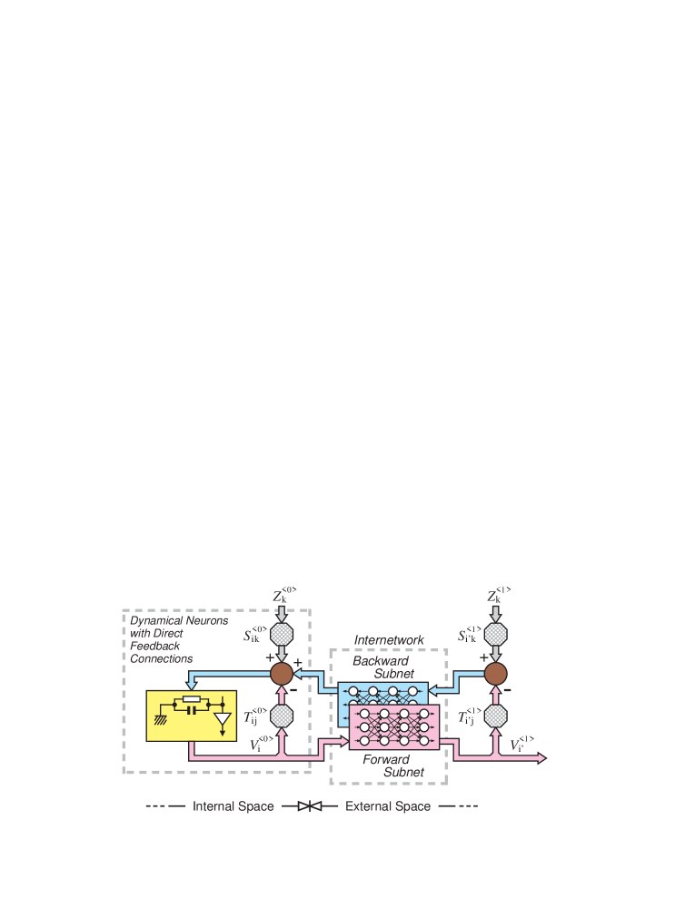
Figure 2: Architecture of the proposed network described by Eqs. (28) and (29), Eqs. (14) and (15), and Eqs. (19), (24), and (27). The network has a pair of a feedback path and an input port in each space. Mapper M and Mapper N shown in Fig. 1 are replaced by a pair of layered networks that are complementary to each other. The computational process of $\delta$ is expressed explicitly as a layered network.

2.3 Learning and Association Modes

As shown in Fig. 2, our model has one feedback path and one input port in both the internal and external spaces. Changing the values of $T_{ij}$ and $S_{ik}$ and their signs in the first and second terms on the right-hand side of the energy function Eq. (3), the shape of the potential field can be chosen arbitrarily. It is reasonable, in this sense, that $T_{ij}$ and $S_{ik}$ are treated as a pair. In the architecture shown by Figs. 1 or 2, $T^{<0>}_{ij}$ and $S^{<0>}_{ik}$ exist in the internal space and $T^{<1>}_{i^{\prime}j}$ and $S^{<1>}_{i^{\prime}k}$ in the external space. For instance, consider a situation where $T^{<0>}_{ij}$ and $S^{<0>}_{ik}$ in the internal space are removed. Then, since there is no inner feedback loop based on $T^{<0>}_{ij}$ and $S^{<0>}_{ik}$, the network dynamics are determined only by a detoured feedback loop with Forward Subnet (or Mapper M), $T^{<1>}_{i^{\prime}j}$ and $S^{<1>}_{i^{\prime}k}$, and Backward Subnet (or Mapper N). How does the network behave in such a limited feedback loop? It is quite interesting to investigate its time-course characteristics. Therefore, prior to studying the model’s behavior in the following sections, we group the model into three topological types as illustrated in Fig. 3, depending on the presence or absence of connections in the internal and external spaces. The upper one is the case with all the connections, and we call it the Learning Mode. The middle and lower types are called the Association Mode; the middle one (Type #0) is the case in which a pair of $T$ and $S$ only exists in the internal space, and the lower one (Type #1) is the case in which it only exists in the external space.

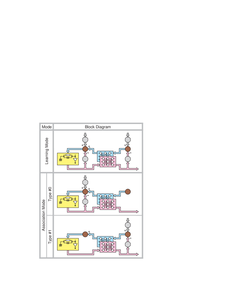
Figure 3: Basically, the model is topologically grouped into two types, totally three types, depending on the presence or absence of connections in the internal and external spaces. The upper row shows the case with all of feedback paths and input ports, and we call it “Learning Mode.” The middle and lower types are called “Association Mode”; the middle one shows the case in which a pair of $T$ and $S$ exists only in the internal space (Type #0), and the lower one does the case in which it only exists in the external space (Type #1).

In the Learning Mode architecture, both an input signal and a target (teaching) signal necessary for learning can be applied to Internetwork. In the Association Mode architectures, on the contrary, either an input signal or a target (teaching) signal appears to be given to Internetwork, so the synaptic connections should not properly be modified. Therefore, it is reasonable in avoiding this situation that we assume a condition in relation to the learining dynamics given by Eq. (29) in our proposed network positioned as a model, when we examine how the activity dynamics differ according to such architectures as Types #0 and #1 in Fig. 3. Thus, the following condition in Eq. (29) is presumed in conjunction with such a topological distinction; Eq. (29) is always ON in the Learning Mode, but it is OFF in the Association Mode, assuming the existence of a certain mechanism. The activity dynamics described by Eq. (28) is ON at all times in both modes.

3 Learning Mode

3.1 Learning Mode in One-Dimensional Model

(1) Linear Mapping

In the network architecture derived in the previous section, only synaptic connections in Internetwork were assumed to have plasticity. Eq. (28) is for the activity dynamics of the whole network, and Eq. (29) is for the learning dynamics on the plastic connections in Internetwork; these two kinds of dynamics run at all times in the network of the Learning Mode. Therefore, we do not need any other particular learning algorithm even when the training issues are discussed for the model, and we should only trace the time-course behavior of the total network when appropriate signals are applied to the input ports.

What kind of signals can we put to those input ports from the outside? For Internetwork to acquire a wide-ranging mapping relationship, we can easily imagine that signals with fixed values are inadequate as inputs in the internal and external spaces. Although we can consider various types of signals, we use a sinusoidal wave as an example of the input signal. Since $V^{<p>}_{i}$ and $Z^{<p>}_{i},~{}(p=0,1)$ are assumed to be of short-time average impulse density, the sinusoidal wave here practically means bursting or semi-bursting nerve impulses. In our first experiment, we applied identical sinusoidal waves to the two input ports in the internal and external spaces of the whole network in Fig. 2, in which the activity dynamics work according to Eq. (28) and the learning dynamics in Internetwork with modifiable synapses run based on Eq. (29). We assume that a dynamical neuron in the internal space has linear input-output characteristics given by Eq. (5) with $\alpha=1.0$. We conduct our simulation studies based on the standard Runge-Kutta method with a stepsize of $0.1~{}{\sf ms}$ which was determined in preliminary studies to yield the correct solution of the equations. We set the values of $c_{i}$ and $\eta_{ij}$ so that the time constants of the activity and learning dynamics are $1~{}{\sf ms}$ and $5~{}{\sf s}$. $r_{i}$ is set to $\infty$. Then, the frequency of both input signals applied in the internal and external spaces is set to $10.0~{}{\sf Hz}$. Each of Forward Subnet and Backward Subnet is assumed to be a three-layered network; we use, in the input and output layers, linear neurons whose characteristics are given by Eq. (5) with $\alpha=1.0$, and in the hidden layer, non-linear ones represented by Eq. (6) with $\alpha=10.0$. In a one-dimensional model, we employ eight hidden neurons in Internetwork.

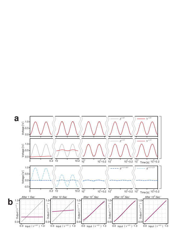
Figure 4: Simulation results for the Linear Case of the Learning Mode in the one-dimensional model. (a) Time-course of network parameters when a set of sinusoidal waves corresponding to the left drawings of Fig. 5 is applied to the input ports in the internal and external spaces. (b) Transition of the input-output relationship acquired in Internetwork. The graphs illustrate the results in which Forward Subnet detached from the model is evaluated at five temporal stages.

Figure 4(a) illustrates the time-course of the network parameters. Here, $T=1.0~{}{\sf S}$ and $S=1.0~{}{\sf S}$. In simulation experiments, we observe the dynamics for $10^{6}$ seconds from the initial state and show the results of five intermediate stages in Fig. 4(a). The upper, middle, and lower graphs respectively denote the input $Z^{<0>}$ and the output $V^{<0>}$ in the internal space, the input $Z^{<1>}$ and the output $V^{<1>}$ in the external space, and the input signal to Backward Subnet $\delta^{<1><3>}$ and the output signal from Backward Subnet $\delta^{<1><0>}$. In the early stage, the figure clearly shows that the output signal from Backward Subnet $\delta^{<1><0>}$ almost equals zero. Therefore, in the internal space without any influence from the other factors, the output of the dynamical neuron $V^{<0>}$ converges smoothly to the input value $Z^{<0>}$ based on its time constant, and $V^{<0>}$ and $Z^{<0>}$ almost overlap. In the external space, on the other hand, the output of Forward Subnet $V^{<1>}$ is very small early on, and differs greatly from the input $Z^{<1>}$. Thus, since the input to Backward Subnet has a large value, learning in Internework progresses adequately; the values of the synaptic connections in it are kept very small in the early stage of the time-course, so the output signal from Backward Subnet remains small. This is why the output in the internal space $V^{<0>}$ almost corresponds to the input from the outside $Z^{<0>}$ as stated above. Learning in Internetwork successfully advances with time; finally $V^{<0>}$ goes to $Z^{<0>}$, as well as $V^{<1>}$ goes to $Z^{<1>}$.

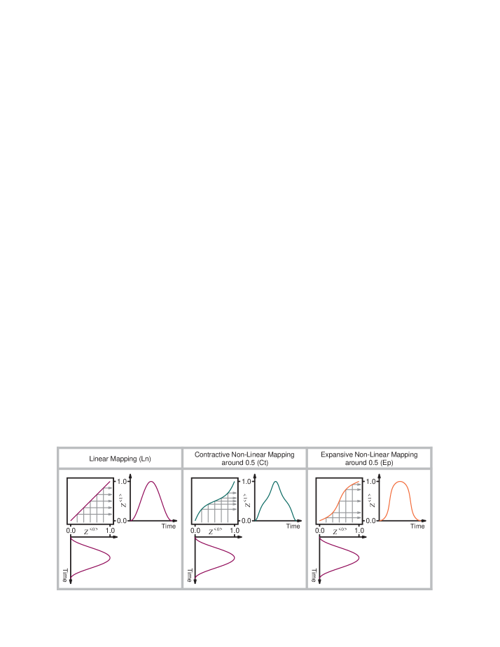
Figure 5: Three sets of sinusoidal and quasi-sinusoidal signals supposed for testing network dynamics in the one-dimensional model. An input signal with sinusoidal waveform for the internal space is converted to that for the external space employing three types of functions.

We can observe very interesting phenomena on the way to the final state, especially $10$ or $10^{2}$ seconds from the beginning. At those times, the maximum amplitude of the output in the internal space $V^{<0>}$ exceeds that of the input in the internal space $Z^{<0>}$. Because the error signal from Backward Subnet $\delta^{<1><0>}$ is added to the dynamical neurons in the internal space, $V^{<0>}$ increases to some extent. Since the architecture and the dynamics of our proposed network model are derived from the energy function, a steeper descent in the energy field is chosen in cooperation with the activity and learning dynamics. This collaborative effect produces a phenomenon in the graphs that contributes to the learning’s acceleration and efficiency. We also investigated how Internetwork can acquire a mapping relationship over time by isolating its part from the model. Figure 4(b) shows the input-output relationships of detached Forward Subnet at five temporal stages. Although a rich input-output relationship is not attained in the early stage, a mapping relationship in Internetwork gradually grows and becomes a complete linear one between $0.0$ and $1.0$.

(2) Non-Linear Mapping

In the previous simulation, we applied identical inputs in the internal and external spaces. It is quite interesting to study situations in which the waveforms of the input signals given to the internal and external spaces are different. As shown in Fig. 5, an input signal with a regular sinusoidal waveform for the internal space is converted to a sinusoidal or quasi-sinusoidal one for the external space using three types of functions. In the middle and right cases, we employ, for non-linear conversion, a function in which a sine wave is superimposed to a straight line $y=x$; the maximal rising or falling inclination of the superimposed sine wave is set here to $0.4$ or $-0.4$.

A regular sine wave used in the experiments for Figs. 4(a) and (b) corresponds to that on the left of Fig. 5, and the pre-converted and post-converted waves are identical since the conversion is due to a linear straight line through the origin; we call this the Linear (Mapping) Case. In contrast, the converting function in the middle case of Fig. 5 is expansive at the edges near $0.0$ and $1.0$ but contractive around $0.5$, so the finally produced periodic signal becomes an acute sinusoidal wave, called the Contractive (Mapping) Case. The converting function on the right of Fig. 5 is contractive at the edges near $0.0$ and $1.0$ but expansive around $0.5$, and the finally produced periodic signal leads to a sinusoidal wave rounded at the end, called the Expansive (Mapping) Case.

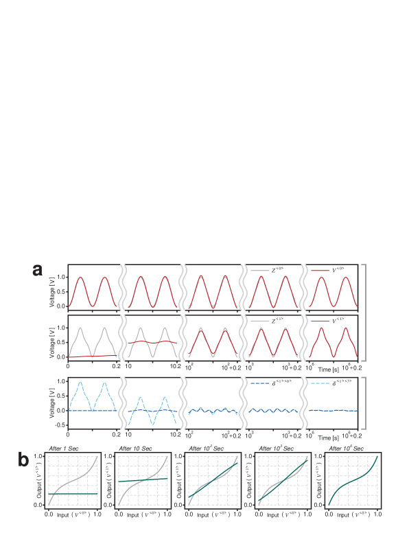
Figure 6: Simulation results for the Contractive Case of the Learning Mode in the one-dimensional model. (a) Time-course of network parameters when a set of sinusoidal and quasi-sinusoidal waves shown in the middle drawings of Fig. 5 is applied to the input ports in the internal and external spaces. (b) Transition of the input-output relationship acquired in Internetwork. The graphs illustrate the results in which Forward Subnet detached from the model is evaluated at five temporal stages.

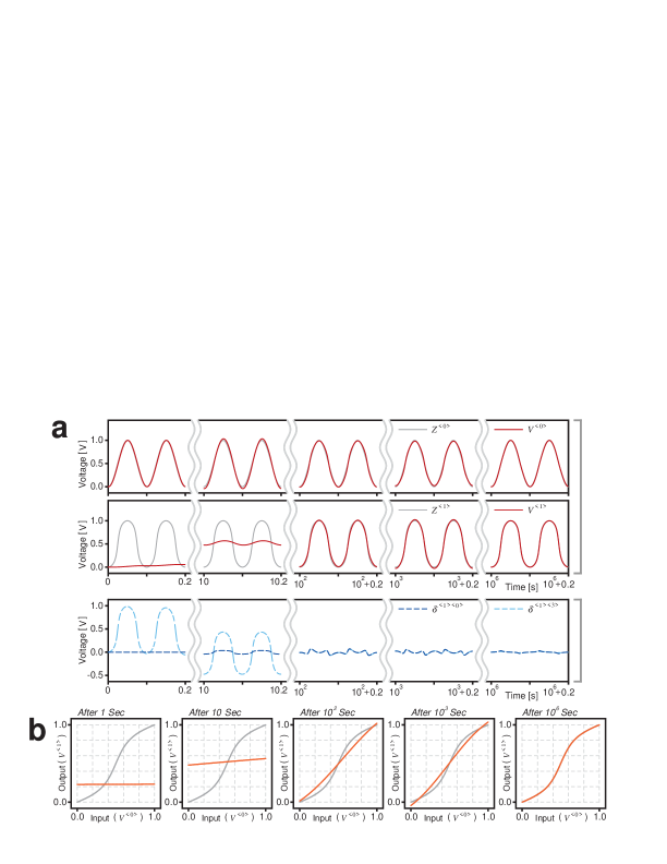
Figure 7: Simulation results for the Expansive Case of the Learning Mode in the one-dimensional model. (a) Time-course of network parameters when a set of sinusoidal and quasi-sinusoidal waves shown in the right drawings of Fig. 5 is applied to the input ports in the internal and external spaces. (b) Transition of the input-output relationship acquired in Internetwork. The graphs illustrate the results in which Forward Subnet detached from the model is evaluated at five temporal stages.

Figure 6 is a simulation result in which we prepared a set of periodic waves in the middle case of Fig. 5, and applied the non-converted sinusoidal wave to the input port in the internal space and the converted one to the input port in the external space, respectively. Here, the frequency of both waves is set to $10.0~{}{\sf Hz}$. Figure 6(a) illustrates the time-course of the states in the model, and Fig. 6(b) shows the transition in the growth of the mapping relationship of Internetwork; both graphs are depicted at five temporal stages as in the case of Figs. 4(a) and (b). Figure 7 shows the simulation result in which a set of periodic waves in the right case of Fig. 5 is applied to the input ports in the internal and external spaces. The frequency of both input signals is also $10.0~{}{\sf Hz}$. Figure 7(a) shows the time-course of the states in the network, and Fig. 7(b) depicts the transition in the growth of the mapping relationship of Internetwork. The varing tendencies of the signals in Figs. 6(a) and (b) or Figs. 7(a) and (b) are basically common to those of Figs. 4(a) and (b), and the outputs $V^{<0>}$ and $V^{<1>}$ correspond respectively to the inputs $Z^{<0>}$ and $Z^{<1>}$ over time. Although the convergence times are different, the input-output relationships to be expected are eventually acquired; the mapping in the middle case of Fig. 5 is obtained in Fig. 6(b), and that in the right case of Fig. 5 is shown in Fig. 7(b).

Scrutinizing the developmental process of these three cases, however, differences and interesting phenomena can be seen. In Figs. 4(a), 6(a), and 7(a), the output in the external space $V^{<1>}$ gradually becomes larger. It does not always exceed the input in the external space $Z^{<1>}$ in Figs. 4(a) and 6(a), although in Fig. 7(a), $V^{<1>}$ slightly exceeds $Z^{<1>}$ after $10^{3}$ seconds. It is also common to Figs. 4(a), 6(a), and 7(a) that, in the internal space after $10$ seconds, the amplitude of $V^{<0>}$ is already slightly larger than that of $Z^{<0>}$. In Fig. 4(a) and Fig. 6(a), the amplitude of the output in the internal space $V^{<0>}$ sometimes further increases and then decreases, but does not go below that of the input in the internal space $Z^{<0>}$. On the contrary, in Fig. 7(a), the amplitude of $V^{<0>}$ continues to gradually decrease after $10$ seconds, and it nearly equals that of $Z^{<0>}$ after $10^{2}$ seconds and is slightly smaller after $10^{3}$ seconds. Specifically, in Fig. 7(a) after $10^{3}$ seconds, the amplitude of the output $V^{<0>}$ is a little smaller than that of the input $Z^{<0>}$ in the internal space, and the amplitude of the output $V^{<1>}$ is slightly larger than that of the input $Z^{<1>}$ in the external space. This situation, that does not appear in Figs. 4(a) and 6(a) of the Linear and Contractive Cases, reflects the acquisition state of the mapping relationship in Internetwork. Seeing Fig. 7(b) after $10^{3}$ seconds, the output of Forward Subnet ranges from $-0.044$ to $1.035$ against the input to Forward Subnet covering the interval from $0.0$ to $1.0$. Such a phenomenon, in which the output exceeds the input once during learning, can generally occur in a static multi-layered neural network without altering the range of input to the network, depending on the training set of the input-output relationship. However, of particular interest is the result in which the proposed network can successfully acquire the mapping relationship on the right of Fig. 5 (Expansive Case) in Internetwork, varying the amplitude of an input signal to Internetwork as mentioned above. Such behavior also seems to be caused by a synergistic effect due to the cooperation of the activity and learning dynamics.

These observations show that, depending on the signal shape of the input from the outside, the mapping relationships acquired in Internetwork as well as the learning speed and how synergistic effects appear are different. This might be caused by qualitative and quantitative differences between signals propagating through Backward Subnet. We will further discuss this point in the following sections.

3.2 Learning Mode in Two-Dimensional Model

(1) Linear Mapping

In this subsection, we consider a two-dimensional model based on the results observed in a one-dimensional model. Since two input signals are necessary for each input port in the internal and external spaces in the two-dimensional model, we have to examine what kind of signals to give to the input ports. When we applied identical sinusoidal waves to the input ports in the internal and external spaces for the one-dimensional model, we obtained a linear mapping relationship that ranged from $0.0$ to $1.0$. If only one kind of sinusoidal wave is applied to four inputs (two inputs for two axes in the internal space and two inputs for two axes in the external space) for the two-dimensional model, instead of a mapping relationship with a two-dimensional extent, one degenerated merely into a single dimension may be acquired. In the following simulation, $T_{ii}=1.0~{}{\sf S}$ and $S_{ii}=1.0~{}{\sf S}$,  $(i=0,1)$, and we set the other $T$ and $S$ values to $0$. In a two-dimensional model, we employ sixteen hidden neurons in Internetwork. The other conditions are basically common to those in the one-dimensional model.

Figure 8 depicts how widely and densely two kinds of sinusoidal waves can cover a two-dimensional plane when one is used to express a point on the horizontal axis and the other on the vertical axis. In terms of acquiring a two-dimensional mapping relation, evenly covering the entire region of the plane is better, and this mechanism is similar to that of the well-known Lissajous curves. Even in simple sinusoidal waves, we can arbitrarily arrange a combination of the frequency and the phase. In Fig. 8, we show an example in which six cases as frequency relationships, $F_{1}=F_{0}$, $F_{1}=(21/20)*F_{0}$, $F_{1}=(20/19)*F_{0}$, $F_{1}=2*F_{0}$, $F_{1}=5*F_{0}$, and $F_{1}=20*F_{0}$ from the upper to the bottom, and four cases as phase relationships, $0^{\circ}$, $90^{\circ}$, $180^{\circ}$, and $270^{\circ}$ from the left to the right are chosen. When the two frequencies are slightly different, e.g., as in the cases of $F_{1}=(21/20)*F_{0}$ and $F_{1}=(20/19)*F_{0}$, the entire region of the plane can evenly be covered. Even though the frequency difference between these two cases is small, each has its own characteristics. The coverage area is not influenced by any phase shifts in the former case, and it becomes denser in the latter case with a phase shift of $90^{\circ}$ or $270^{\circ}$ in particular. When $F_{0}$ and $F_{1}$ have a frequency relation of integral multiples, in contrast, the coverage area becomes wider and denser with the increase of its multiple ratio, although it is subject to the influence of the phase difference especially in the case of a small ratio of integral multiples. We chose three cases, $F_{1}=(20/19)*F_{0}$, $F_{1}=20*F_{0}$, and $F_{1}=5*F_{0}$ without any phase shifts, and evaluated how their network states vary with the progress of the total dynamics.

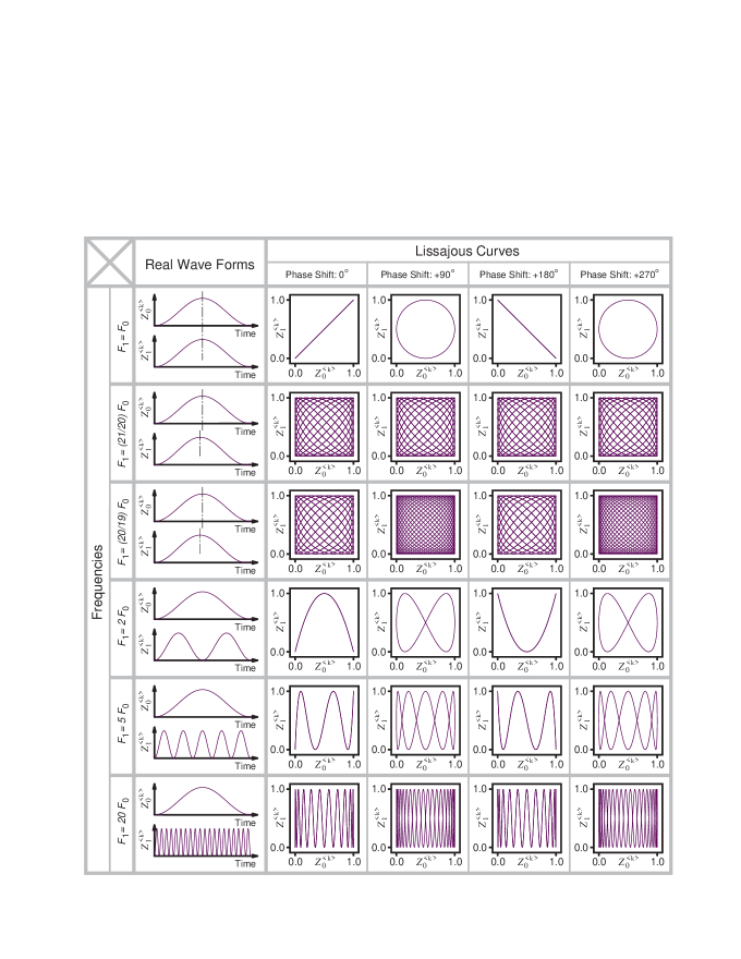
Figure 8: Relationship between two kinds of sinusoidal waves with different frequencies and phases in the Linear Case. The graphs show how widely and densely two signals for horizontal and vertical axes can cover a two-dimensional plane. Note the similarity to Lissajous curves.

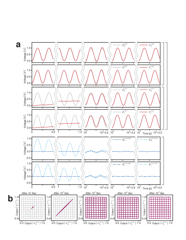
Figure 9: Simulation results for the Linear Case of the Learning Mode in the two-dimensional model. Frequency relationship between two sinusoidal waves for horizontal and vertical axes is $F_{1}=(20/19)*F_{0}$. (a) Time-course of network parameters. (b) Transition of the input-output relationship acquired in Internetwork (detached Forward Subnet).

Figure 9 shows an example with $F_{1}=(20/19)*F_{0}$, in which a non-distorted regular sinusoidal wave with $9.5~{}{\sf Hz}$ is applied to $Z^{<0>}_{0}$ and $Z^{<1>}_{0}$ for the horizontal axes, and that with $10.0~{}{\sf Hz}$ is given to $Z^{<0>}_{1}$ and $Z^{<1>}_{1}$ for the vertical axes. Figure 9(a) illustrates the time-course at the signal level, and Fig. 9(b) depicts the progress of the mapping relationship acquired in Internetwork on the total dynamics. In Fig. 9(a), the phases of $Z^{<0>}_{0}$ and $Z^{<1>}_{0}$ from $1.0~{}{\sf s}$ to $1.2~{}{\sf s}$ are roughly opposite of those from $0.0~{}{\sf s}$ to $0.2~{}{\sf s}$; this is because one period of the signal with $9.5~{}{\sf Hz}$ is $2/19$ seconds. In the two-dimensional model, both activity and learning dynamics progress cooperatively and smoothly through such a stage that the amplitudes of $V^{<0>}_{0}$ and $V^{<0>}_{1}$ exceed those of $Z^{<0>}_{0}$ and $Z^{<0>}_{1}$ in the same way as the one-dimensional model. In the end, the outputs in the external space $V^{<1>}_{0}$ and $V^{<1>}_{1}$ almost coincide with the inputs in the external space $Z^{<1>}_{0}$ and $Z^{<1>}_{1}$. From the viewpoint of the acquisition of the mapping relationship in Internetwork, the progress over time is very smooth as shown in Fig. 9(b). Internetwork finally acquires a two-dimensional linear mapping within a range strictly from $0.0$ to $1.0$. When we concentrate on the state after $10^{2}$ seconds in Fig. 9(a), the learning of Internetwork appears to be already well-advanced, judging from the situation in which the amplitudes of $V^{<1>}_{0}$ and $V^{<1>}_{1}$ become fairly large. However, this is not the case. By carefully looking at the signals $V^{<1>}_{0}$ and $V^{<1>}_{1}$, $V^{<1>}_{0}$ moves to the left of $Z^{<1>}_{0}$ and seems to be going to a higher frequency, and in contrast, $V^{<1>}_{1}$ goes to the right of $Z^{<1>}_{1}$ and appears to be moving to a lower frequency. This behavior creates an effect in which the frequencies of two input signals applied for the horizontal and vertical axes are getting closer to each other, although the intervals between zero-crossings remain constant and those frequencies do not actually change at all. Checking the state after $10^{2}$ seconds in Fig. 9(b), the mapping relationship obtained at this moment is not two-dimensional; it remains almost on a one-dimensional straight line. This phenomenon, in which such an interesting way of learning is chosen, also reflects the mutual interaction of the activity and learning dynamics derived from the energy function through its minimizing procedure.

(2) Non-Linear Mapping

Assuming quasi-sinusoidal waves in the middle panel of Fig. 5 (the Contractive Case), Fig. 10 shows, in a way similar to Fig. 8, how widely and densely those signals with various relations between frequencies and phases can cover a two-dimensional plane. The relations between frequencies and phases basically resemble those in Fig. 8. However, even if the relation between frequencies is the same as the case with non-distorted sinusoidal waves, some areas become denser and others are sparser depending on the degree of non-linearity for a converting function.

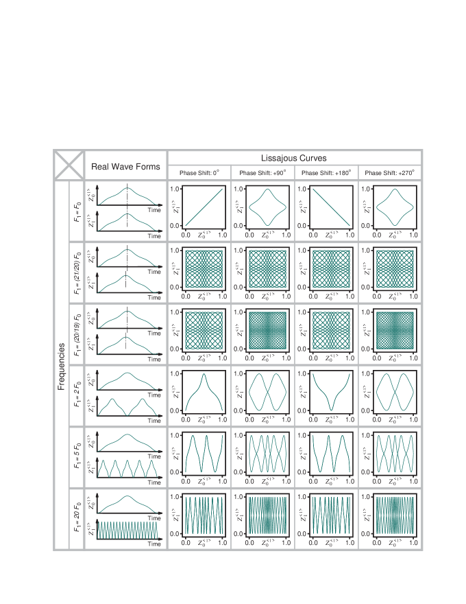
Figure 10: Relationship between two kinds of quasi-sinusoidal waves with different frequencies and phases in the Contractive Case. The graphs show how widely and densely two signals for horizontal and vertical axes can cover a two-dimensional plane. Also note the similarity to Lissajous curves.

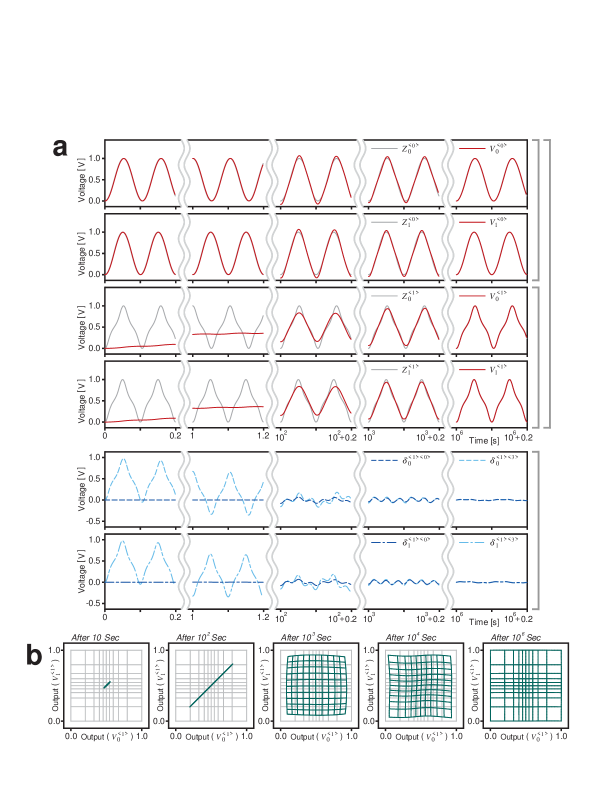
Figure 11: Simulation results for the Contractive Case of the Learning Mode in the two-dimensional model. Frequency relationship between two quasi-sinusoidal waves for horizontal and vertical axes is $F_{1}=(20/19)*F_{0}$. (a) Time-course of network parameters. (b) Transition of the input-output relationship acquired in Internetwork (detached Forward Subnet).

Figure 11 shows a simulation result with $F_{1}=(20/19)*F_{0}$ under no phase shift, in which the non-distorted regular sinusoidal waves with $9.5~{}{\sf Hz}$ for the horizontal axis and $10.0~{}{\sf Hz}$ for the vertical axis are respectively applied to $Z^{<0>}_{0}$ and $Z^{<0>}_{1}$, and the distorted sinusoidal waves of the Contractive Case with $9.5~{}{\sf Hz}$ for the horizontal axis and $10.0~{}{\sf Hz}$ for the vertical axis are respectively put to $Z^{<1>}_{0}$ and $Z^{<1>}_{1}$. Figure 11(a) shows the time-course of the dynamics at the signal level, and Fig. 11(b) shows the transition of the mapping relationship in Internetwork over time. As is clear in Figs. 11(a) and (b), a mapping relationship that is contractive around $0.5$ and expansive at the edges near $0.0$ and $1.0$ was successfully acquired through such a stage that the amplitudes of $V^{<0>}_{0}$ and $V^{<0>}_{1}$ exceed those of $Z^{<0>}_{0}$ and $Z^{<0>}_{1}$ after $10^{2}$ seconds. As for the mapping of the Contractive Case, the learning speed tends to be slower in the same way as in the one-dimensional model, and this is quite obvious from a comparison of the states after $10^{3}$ seconds from the beginning in Figs. 9(b) and 11(b).

When quasi-sinusoidal waves in the right panel of Fig. 5 (the Expansive Case) are employed, Fig. 12 depicts how widely and densely they can cover a two-dimensional plane. In a way similar to Fig. 10, some areas are denser but others are sparser for the relation between lines. Note, however, that the area where information necessary for learning is densely applied changes depending on the quantitative differences of the non-linearity; the relations between the denser and sparser areas are reversed in Figs. 10 and 12, on the basis of Fig. 8 without any distortion of waves.

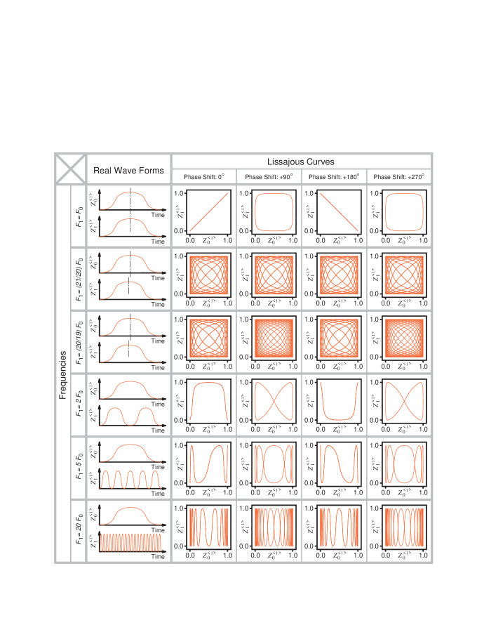
Figure 12: Relationship between two kinds of quasi-sinusoidal waves with different frequencies and phases in the Expansive Case. The graphs show how widely and densely two signals for horizontal and vertical axes can cover a two-dimensional plane. Also note the similarity to Lissajous curves.

Figure 13 shows a simulation result with $F_{1}=20*F_{0}$ under no phase shift, in which the relationship between frequencies $F_{0}$ and $F_{1}$ is quite unlike the above examples in the two-dimensional model. The non-distorted regular sinusoidal waves with $0.5~{}{\sf Hz}$ for the horizontal axis and $10.0~{}{\sf Hz}$ for the vertical axis are respectively applied to $Z^{<0>}_{0}$ and $Z^{<0>}_{1}$, and the distorted sinusoidal waves in the Expansive Case with $0.5~{}{\sf Hz}$ for the horizontal axis and $10.0~{}{\sf Hz}$ for the vertical axis are respectively put to $Z^{<1>}_{0}$ and $Z^{<1>}_{1}$. Figure 13(a) is the time-course of the dynamics at the signal level. Comparing Fig. 13(a) with Fig. 9(a) or Fig. 11(a), the frequency of $F_{1}$ in Fig. 13(a) seems extremely high at a glance, but $F_{1}$ is commonly set to $10.0{\sf Hz}$, and note that this impression is caused by the lower value setting of $F_{0}$. Figure 13(b) shows the transition of the mapping relationships acquired in Internetwork over time. As is clear from this result, also in the case of $F_{1}=20*F_{0}$, a complete mapping relationship that is expansive around $0.5$ and contractive at the edges near $0.0$ and $1.0$ can finally be acquired in Internetwork.

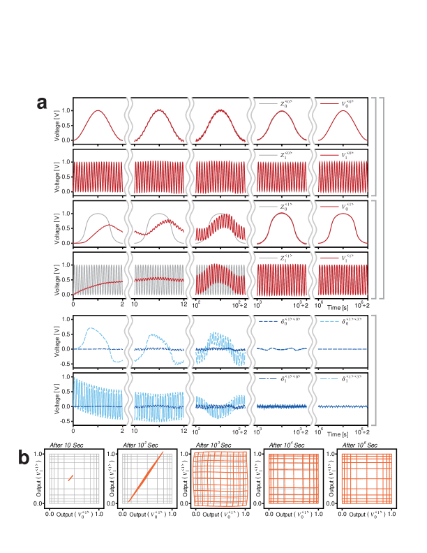
Figure 13: Simulation results for the Expansive Case of the Learning Mode in the two-dimensional model. Frequency relationship between two quasi-sinusoidal waves for horizontal and vertical axes is $F_{1}=20*F_{0}$. (a) Time-course of network parameters. (b) Transition of the input-output relationship acquired in Internetwork (detached Forward Subnet).

Thus, we conclude that a two-dimensional mapping relationship between the internal and external spaces can successfully be obtained depending on the degree of the non-linear warping for periodic signals applied to the input ports in the internal and external spaces, when $F_{0}$ and $F_{1}$ have such a relation that either they are slightly different (Fig. 8 and Figs. 9(a) and (b) or Fig. 10 and Figs. 11(a) and (b)) or very different (Fig. 12 and Figs. 13(a) and (b)).

When the frequency relationship between $F_{0}$ and $F_{1}$ takes a low integral multiple, such as $F_{1}=2*F_{0}$ or $F_{1}=5*F_{0}$ in Fig. 12, how do the network dynamics progress over time and what kind of results can be obtained? Figure 14 shows a simulation result with $F_{1}=5*F_{0}$ under no phase shift. Non-distorted regular sinusoidal waves with $2.0~{}{\sf Hz}$ for the horizontal axis and $10.0~{}{\sf Hz}$ for the vertical axis are respectively applied to $Z^{<0>}_{0}$ and $Z^{<0>}_{1}$, and the distorted sinusoidal waves in the Expansive Case with $2.0~{}{\sf Hz}$ for the horizontal axis and $10.0~{}{\sf Hz}$ for the vertical axis are respectively put to $Z^{<1>}_{0}$ and $Z^{<1>}_{1}$. Figure 14(a) indicates the time-course of the dynamics at the signal level, and Fig. 14(b) shows the transition of the mapping relationship in Internetwork over time. As is clear in Fig. 14(a), even when $F_{0}$ and $F_{1}$ are related with a small integral multiple, the outputs in the external space $V^{<1>}_{0}$ and $V^{<1>}_{1}$ eventually overlap with the inputs in the external space $Z^{<1>}_{0}$ and $Z^{<1>}_{1}$. As shown in Fig. 14(b), however, a complete two-dimensional mapping relation is not obtained, compared with the $F_{1}=20*F_{0}$ case illustrated in Fig. 13(b). Note the $F_{1}=5*F_{0}$ case with no phase shift in Fig. 12 again. For this frequency relation, the information effective for learning is sparse within the square two-dimensional plane, and its situation seems to cause the above phenomenon. It is not hard to imagine that the result worsens when $F_{1}=2*F_{0}$. Even for this $F_{1}=5*F_{0}$, the simulation results changes depending on the number and the gain of the hidden units in Internetwork. In any cases, when $F_{0}$ and $F_{1}$ are related with a small integral multiple, the activity and learning dynamics themselves progress smoothly to a final state, but the mapping relationship acquired in Internetwork does not become rich with all the generalization capability of a layered neural network.

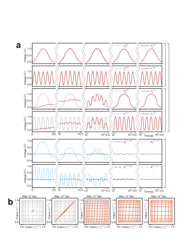
Figure 14: Simulation results for the Expansive Case of the Learning Mode in the two-dimensional model. Frequency relationship between two quasi-sinusoidal waves for horizontal and vertical axes is $F_{1}=5*F_{0}$. (a) Time-course of network parameters. (b) Transition of the input-output relationship acquired in Internetwork (detached Forward Subnet).

4 Association Mode

4.1 Association Mode in One-Dimensional Model

In our model, as stated in Subsection 2.3, we distinguish two modes, Learning and Association, that depend on whether pairs (or just one pair) of a feedback path and an input port exist(s) in the internal and/or external space(s). In this section, we describe the dynamical behavior of the Association Mode in which Eq. (29) is supposed to be OFF and all other conditions are shared with those in Section 3. Let us consider the one-dimensional model first.

Figure 15 shows the time-course of the network states from four initial points, when a pair of a feedback path and an input port exists only in the internal space (Type #0 in Fig. 3) and a fixed value of $0.5$ is applied as an input for the internal space. The obtained results are shown as a table with three rows. The upper row is the Contractive Case with a mapping relationship that is obtained by the simulation shown in Fig. 6, the middle one is the Linear Case based on the simulation shown in Fig. 4, and the lower one is the Expansive Case based on the simulation shown in Fig. 7. For the horizontal direction, each of the leftmost graphs shows the time-course of the output in the internal space, its right one is the mapping relationship already acquired in Internetwork, the next right one shows the time-course of the output in the external space, and the rightmost one depicts the time-course of the output from Backward Subnet. To focus on the initial responses, we only plot the variations for $4~{}{\sf ms}$ from the beginning. Also to help grasp the meaning of each graph, we draw a block diagram of the whole network with gray wide arrow lines in the upper part and append an index to each graph. As is clear from 15-Ct-DL, 15-Ln-DL, and 15-Ep-DL, in this Association Mode with a pair of a feedback path and an input port only in the internal space, no signal propagates through Backward Subnet in principle. So the output in the internal space $V^{<0>}$ is simply converted in a static manner to the output in the external space $V^{<1>}$ by Forward Subnet. Therefore, in the Contractive Case in the upper row, for instance, external 15-Ct-V<1> is entirely contractive against internal 15-Ct-V<0>, and in the Expansive Case in the lower row, external 15-Ep-V<1> is expansive overall to internal 15-Ep-V<0>. In the Linear Case in the middle row, on the contrary, the internal 15-Ln-V<0> and external 15-Ln-V<1> graphs are completely the same.

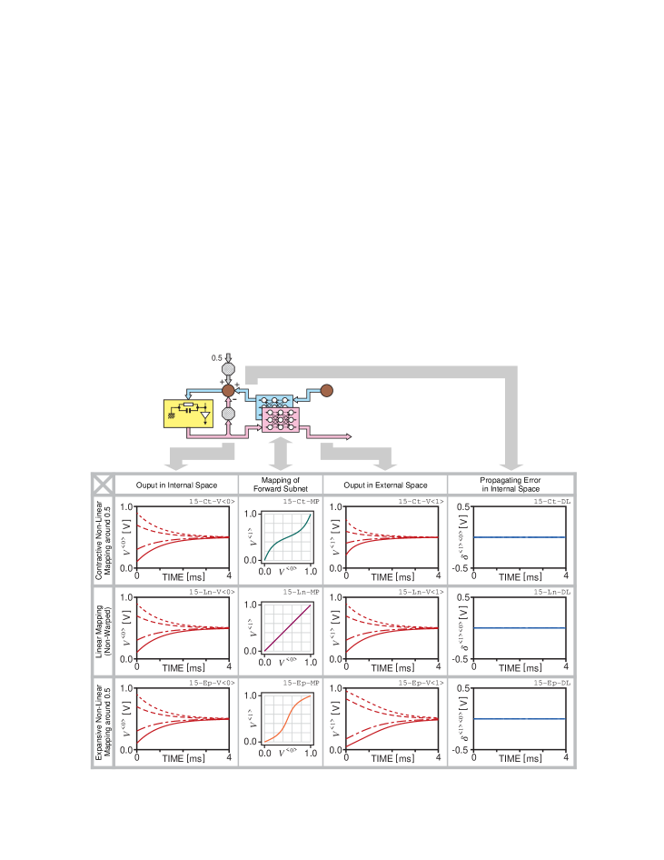
Figure 15: Simulation results for Type #0 of the Association Mode in the one-dimensional model. In this experiment, the place with a pair of a feedback path and an input port is limited to the internal space. The graphs include the Contractive, Linear, and Expansive Cases.

Next, we consider the network behavior when a pair of a feedback path and an input port exists only in the external space. Notice the signal propagating through Backward Subnet in this case. Figure 16 illustrates what kind of signal flows through Backward Subnet for three mapping cases of Internetwork. The lower right figure shows the linkage between a block diagram of the corresponding part and signal flows, and the lower left graph is the relation between the signals \scriptsize1⃝ and \scriptsize2⃝. The upper five graphs depict the relation between the output from Forward Subnet \scriptsize2⃝ and that from Backward Subnet \scriptsize4⃝, choosing five values as the input from the outside \scriptsize3⃝. Since the upper five graphs and the lower left figure are related with signal \scriptsize2⃝, we supplement their relation using multiple dashed arrow lines with different gray levels and widths. In the lower left and upper five graphs, green means the Contractive Case, orange corresponds to the Expansive Case, and purple indicates the Linear Case.

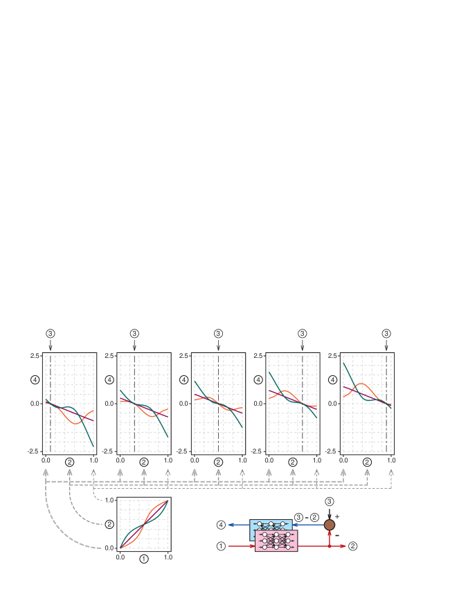
Figure 16: A conceptual diagram and graphs describing signal flows through Backward Subnet in Type #1 of the Association Mode. The lower right drawings show the relation between a block diagram of the corresponding part and signal flows. The lower left graph indicates the input-output relation in Forward Subnet. The upper five graphs show the relation between the output from Forward Subnet and that from Backward Subnet, choosing five values as the input from the outside. In the lower left graph and the upper five graphs, green, purple, and orange correspond to the Contractive, Linear, and Expansive Cases.

The output in the internal space \scriptsize1⃝ is converted to the output in the external space \scriptsize2⃝ by Forward Subnet. Computing the subtraction of \scriptsize2⃝ from \scriptsize3⃝, \scriptsize3⃝ - \scriptsize2⃝ is applied to Backward Subnet, where, as is clear from Eq. (13) in general, the product-sum operation of $\partial V^{<1>}_{i^{\prime}}/\partial V^{<0>}_{i}$ and ( \scriptsize3⃝ - \scriptsize2⃝ ) for $i^{\prime}$ is executed. Since the number of $i$ and $i^{\prime}$ elements is assumed to be one each in this explanation, what is multiplied by ( \scriptsize3⃝ - \scriptsize2⃝ ) is simply $\partial V^{<1>}/\partial V^{<0>}$, which means how warped the mapping relationship is in Forward Subnet on the basis of the Linear Case.

Let us consider the case with $\mbox{\scriptsize3⃝}=0.5$ that corresponds to the center graph in the upper ones of Fig. 16. In the Contractive Case with the green lines, a signal propagating through Backward Subnet \scriptsize4⃝ becomes very small when \scriptsize2⃝ is around $0.5$, since the value of ( \scriptsize3⃝ - \scriptsize2⃝ ) and inclination $\partial V^{<1>}/\partial V^{<0>}$ are both small. In addition, it is important that the curve of \scriptsize4⃝ becomes an inflection point when $\mbox{\scriptsize2⃝}=0.5$. This produces a very unfavorable effect on the convergence dynamics of the whole network. At the edges near $0.0$ and $1.0$ in \scriptsize2⃝, on the other hand, the value of \scriptsize4⃝ sent to the internal space by Backward Subnet is fairly large, since both ( \scriptsize3⃝ - \scriptsize2⃝ ) and $\partial V^{<1>}/\partial V^{<0>}$ become large at the same time. In the Expansive Case with the orange lines, $\partial V^{<1>}/\partial V^{<0>}$ is large around $0.5$, but it is conversely small at the edges near $0.0$ and $1.0$. The value of \scriptsize4⃝, which is sent to the internal space by Backward Subnet, is the product of $\partial V^{<1>}/\partial V^{<0>}$ and ( \scriptsize3⃝ - \scriptsize2⃝ ). As a result, \scriptsize4⃝ has two peaks between $0.0$ and $0.5$ and between $0.5$ and $1.0$. The value of \scriptsize4⃝ doesn’t remain small even when \scriptsize2⃝ is close to $0.5$, so Internetwork in the Expansive Case seems to have an advantageous effect on the convergence dynamics of the whole network. These characteristics are basically common to the case of $\mbox{\scriptsize3⃝}\neq 0.5$, and a signal transmitted to the internal space by Backward Subnet varies in many ways, depending on whether Forward Subnet has contractive or expansive mapping. In the Linear Case, $\partial V^{<1>}/\partial V^{<0>}$ is a constant with value $1$, so \scriptsize4⃝ is proportional to ( \scriptsize3⃝ - \scriptsize2⃝ ); in the upper five graphs of Fig. 16, the purple lines are all straight.

Figure 17 shows the time-course of the network states when the fixed value of $0.5$ is applied as an input for the external space in an Association Mode, in which a pair of a feedback path and an input port exists only in the external space (Type #1 in Fig. 3). In the same manner as in Fig. 15, the results are depicted as a table with three rows. The upper row indicates the Contractive Case with a mapping relationship that is obtained by the computation shown in Fig. 6, the middle one is the Linear Case obtained by the computation in Fig. 4, and the lower one shows the Expansive Case obtained by the computation in Fig. 7. For the horizontal direction, the arrangement of graphs is the same as that in Fig. 15. In this Association Mode, as stated above using Fig. 16, a signal flows through Backward Subnet. Therefore, this behavior is fairly different from that of Fig. 15 with a pair of a feedback path and an input port only in the internal space.

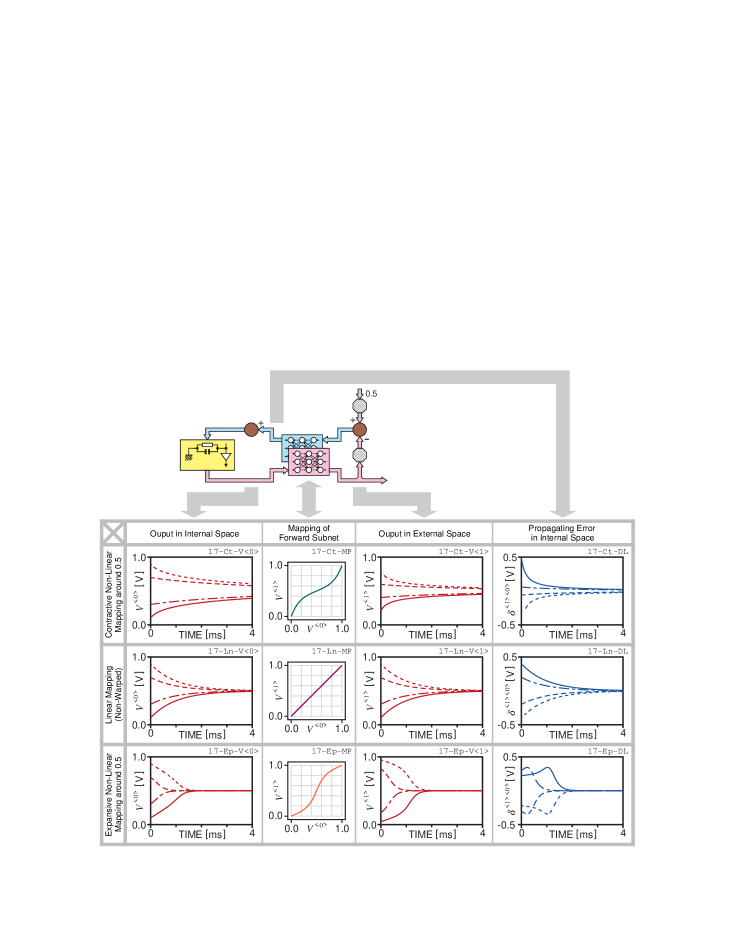
Figure 17: Simulation results for Type #1 of the Association Mode in the one-dimensional model. In this experiment, the place with a pair of a feedback path and an input port is limited to the external space. The graphs also include the Contractive, Linear, and Expansive Cases.

Notice the upper row of the Contractive Case. It is common to Fig. 15 that external 17-Ct-V<1> is contractive overall compared with internal 17-Ct-V<0>. When the output of the internal space in the early stage exists within the expansive mapping domain, the signal propagating through Backward Subnet is rather large, but it becomes drastically smaller after the network state moves to the contractive mapping domain, and its convergence slows down as it approaches $0.5$. Therefore, the effect that makes an error signal (an input from the outside - an output via a feedback connection) in the external space reduce in the internal space becomes smaller and smaller over time. As a result, the output in the external space $V^{<1>}$ converges very slowly toward $0.5$. We can also understand this phenomenon from the actual output of Backward Subnet $\delta^{<1><0>}$ as shown in 17-Ct-DL.

In the lower row of the Expansive Case, as in the lower row of Fig. 15, external 17-Ep-V<1> is more expansive than internal 17-Ep-V<0>. In this mapping case, produced is an effect that moves an error signal from the external space to the internal space and strongly reduces it there, since a signal flowing through Backward Subnet retains its large value even around $0.5$. As a result, both network states in the internal and external spaces converge quickly to the input value of $0.5$. As indicated by the orange lines in Fig. 16, a signal propagating to the internal space via Backward Subnet \scriptsize4⃝ is not monotonous but has two peaks between $0.0$ and $0.5$ and between $0.5$ and $1.0$. Interestingly, due to this, the decreasing behavior of the error signal $\delta^{<1><0>}$ changes on the way, as shown in 17-Ep-DL.

In the middle row of the Linear Case, an input to and an output from Forward Subnet are identical, and the dynamics in this Association Mode are also the same as the case of Fig. 15 without any feedback signals via Forward Subnet and Backward Subnet.

4.2 Association Mode in Two-Dimensional Model

In this subsection, we check the network behavior for the Association Mode in the two-dimensional model. Figure 18 shows the network’s time-course with a pair of a feedback path and an input port only in the internal space (Type #0 in Fig. 3), when fixed values $(0.5,0.5)$ are applied to the input port in the internal space. In the same way as in Figs. 15 and 17, the results are illustrated as a table with three rows. The upper row is for the network in the Contractive Case with Internetwork obtained by the simulation shown in Fig. 11, the middle one is for the network in the Linear Case with that obtained in Fig. 9, and the lower one is for the network in the Expansive Case with that obtained in Fig. 13. For the horizontal direction, each of the left graphs is the time-course of the output in the internal space, its right one shows the mapping relationship already acquired in Internetwork, and the rightmost one shows the time-course of the output in the external space. Here, we omit inputs and outputs to/from Backward Subnet that were shown in the one-dimensional model. In the graphs, small black circles indicate the initial points, 16 of which were selected for each case; all 16 initial points are arranged in such a manner that their positions in the internal spaces are common throughout the three cases. We chose five trajectories in each graph and drew ten small subsidiary arrows at most on each of those trajectories every $0.2~{}{\sf ms}$; a longer interval between the arrows means a faster change with time.

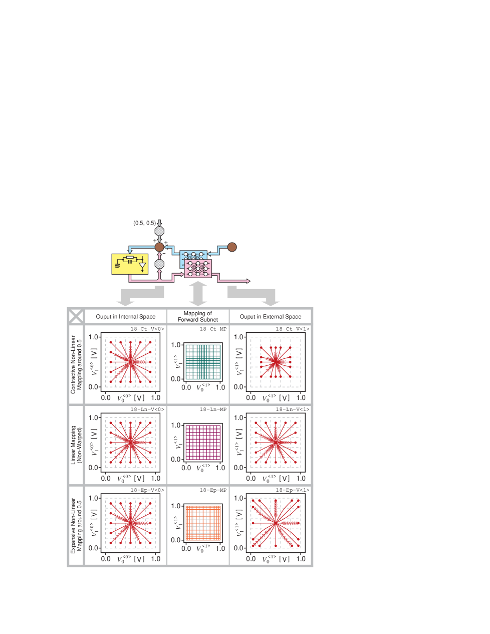
Figure 18: Simulation results for Type #0 of the Association Mode in the two-dimensional model. In this experiment, the place with a pair of a feedback path and an input port is limited to the internal space. The graphs include the Contractive, Linear, and Expansive Cases.

For this Association Mode with a pair of a feedback path and an input port only in the internal space, as in the one-dimensional model, signals through Backward Subnet do not exist. Therefore, the output in the internal space $V^{<0>}_{i}$ is mapped simply and statically to that in the external space $V^{<1>}_{i^{\prime}}$ by Forward Subnet. Due to this, in the Linear Case shown in the middle row, the initial positions, the (straight) trajectories, and the convergent ways (intervals between arrows) of the outputs are identical in the internal and external spaces.

How is the Contractive Case shown in the upper row? On the basis of the case shown in the middle row, we summarize its convergence characteristics as follows:

• The initial points in the external space are located nearer to the center $(0.5,0.5)$ than those in the internal space.

• When the initial points are on a diagonal line connecting $(0.0,0.0)$ and $(1.0,1.0)$, or on that between $(0.0,1.0)$ and $(1.0,0.0)$, $V^{<1>}_{0}$ and $V^{<1>}_{1}$ vary in the same manner, and so the network state converges straightforwardly to the center.

• When the initial points are on a straight line between $(0.0,0.5)$ and $(1.0,0.5)$, or on that connecting $(0.5,0.0)$ and $(0.5,1.0)$, the varing tendencies of $V^{<1>}_{0}$ and $V^{<1>}_{1}$ are different from each other, but the network state converges straightforwardly to the center, since one parameter already remains in a converging state and only the other parameter varies.

• As for the other initial positions except for the case of (0-b) and (0-c), $V^{<1>}_{0}$ and $V^{<1>}_{1}$ vary in different ways, and the network state converges in a curved path to the center. Then the curved line bends in the direction with a steep gradient, in such a manner that the network state gets closer to a neighbor straight line $V^{<1>}_{1}=V^{<1>}_{0}$ or $V^{<1>}_{1}=-V^{<1>}_{0}+1.0$.

• Overall, the output in the external space 18-Ct-V<1> is a reduced-size version of 18-Ct-V<0> according to the mapping relationship of Forward Subnet.

In the Expansive Case shown in the lower row, (0-b) and (0-c) are shared, but the behavior in (0-a), (0-d), and (0-e) is different from that in this case as follows:

• The initial positions in the external space are located farther from the center compared with the Contractive and Linear Cases.

• As for the other initial positions except for the cases in (0-b) and (0-c), $V^{<1>}_{0}$ and $V^{<1>}_{1}$ vary in different ways, and the network state converges in a curved path to the center. But their curving tendencies are opposite to those in the Contractive Case of the upper row; the network state approaches a straight line $V^{<1>}_{0}=0.5$ or $V^{<1>}_{1}=0.5$.

• Contrary to the Contractive Case, the output in the external space 18-Ep-V<1> is an extended-size version of 18-Ep-V<0> based on the mapping relationship of Forward Subnet. The intervals between arrows in 18-Ep-V<1> are almost equal before $2~{}{\sf ms}$, because the convergence speed in the edges near $0.0$ and $1.0$ is suppressed due to the contractive mapping relationship in those domains. This phenomenon can easily be imagined from the straightforward variation during $0~{}{\sf ms}-2~{}{\sf ms}$ in the one-dimensional model of 15-Ep-V<1>.

On the other hand, Fig. 19 illustrates the behavior of a network with a pair of a feedback path and an input port only in the external space (Type #1 in Fig. 3), when fixed values $(0.5,0.5)$ are applied to the input port in the external space. The results are summarized as three rows as in Fig. 18. The upper row means the Contractive Case with Internetwork obtained through the computation in Fig. 11, the middle one is the Linear Case with that in Fig. 9, and the lower one is the Expansive Case with that in Fig. 13. For the horizontal direction, the arrangement of graphs is the same as that in Fig. 18. The 16 initial positions in each case are set to be equivalent in the internal space. The information for the inputs and outputs to/from Backward Subnet is also omitted in the figure. Since the signals through Backward Subnet exist in this Association Mode, the state variation in the external space should affect that in the internal space. First, let us check the Linear Case in the middle row. The information for the feedback and the input in the external space is sent to the internal space as it is. So in the one-dimensional model, 15-Ln-V<0> and 15-Ln-V<1> in the middle row of Fig. 15 were the same, as were 17-Ln-V<0> and 17-Ln-V<1> in the middle row of Fig. 17. In the two-dimensional model, 19-Ln-V<0> and 19-Ln-V<1> are identical to each other and are equal to 18-Ln-V<0> and 18-Ln-V<1> of Fig. 18.

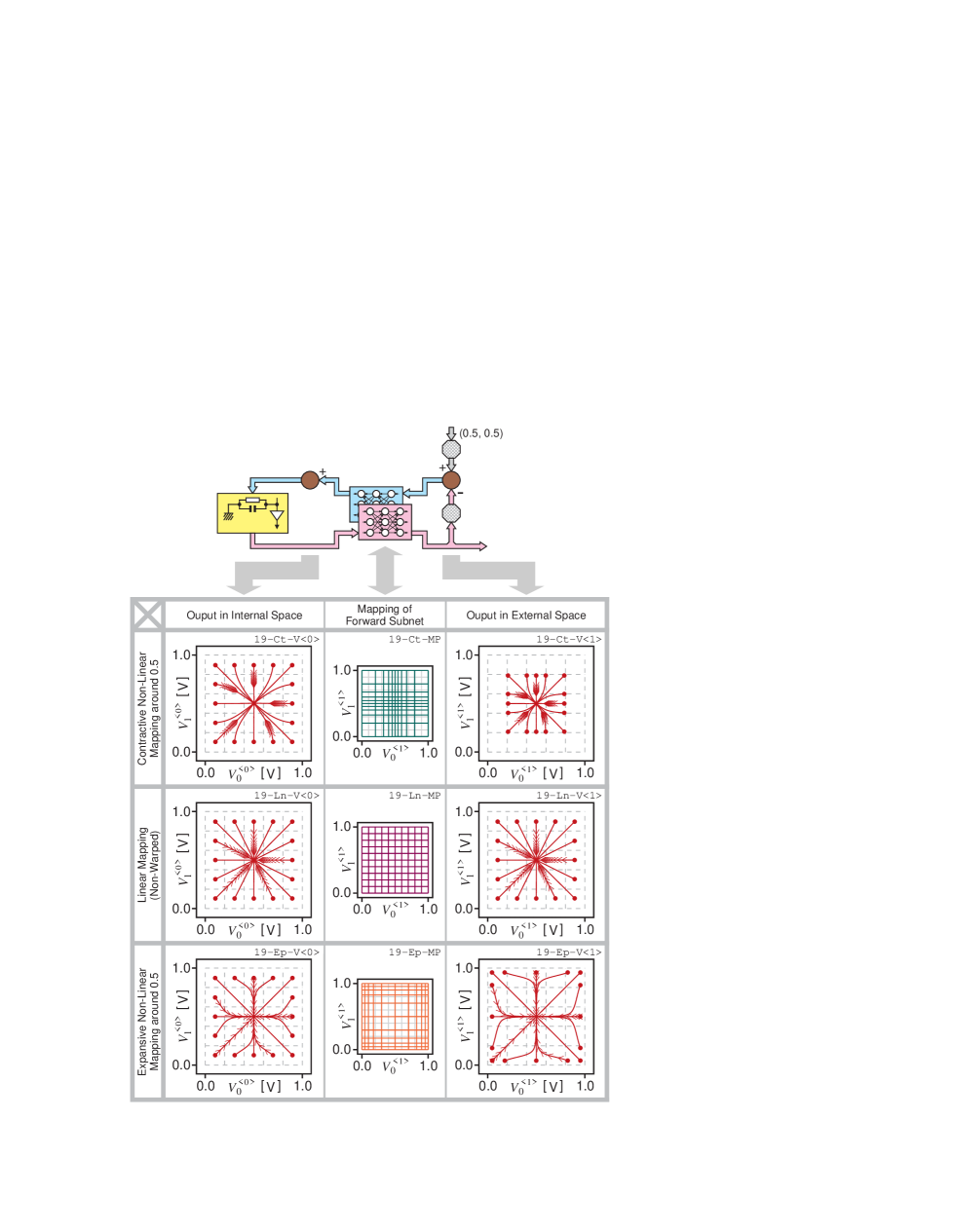
Figure 19: Simulation results for Type #1 of the Association Mode in the two-dimensional model. In this experiment, the place with a pair of a feedback path and an input port is limited to the external space. The graphs also include the Contractive, Linear, and Expansive Cases.

Next, on the basis of these results in the middle rows, we check the Contractive Case in the upper row. The convergence characteristics can be itemized as follows:

• The initial positions in the external space are located nearer to the center as with (0-a).

• When an initial position is located on a diagonal line connecting $(0.0,0.0)$ with $(1.0,1.0)$, or on that between $(0.0,1.0)$ and $(1.0,0.0)$, the network state converges linearly to the center since $V^{<1>}_{0}$ and $V^{<1>}_{1}$ vary with the same tendency.

• When an initial point is located on a straight line between $(0.0,0.5)$ and $(1.0,0.5)$, or on that between $(0.5,0.0)$ and $(0.5,1.0)$, the network state also converges linearly to the center since either $V^{<1>}_{0}$ or $V^{<1>}_{1}$ has already converged on a fixed value and the other only varies.

• Except for the initial points in (1-b) and (1-c), the network state goes to the center in a curved line, since $V^{<1>}_{0}$ and $V^{<1>}_{1}$ vary with mutually different tendencies based on the mapping relationship of Forward Subnet; the network state varies toward the center in such a manner that it approaches a diagonal line where $V^{<1>}_{1}=V^{<1>}_{0}$ or $V^{<1>}_{1}=-V^{<1>}_{0}+1.0$. Then the variation occurring in the external space is returned to the internal space by Backward Subnet, and further transmitted to the external space through Forward Subnet. Due to this looping, the convergence trajectory in the internal space curves, and that in the external space curves more; this result is obvious by comparing 19-Ct-V<0> and 19-Ct-V<1> with 18-Ct-V<0> and 18-Ct-V<1> of Fig. 18.

• It is common to Fig. 18 that the network state in the external space is contractive overall compared with that in the internal space. But as the output in the external space approaches the center, the corresponding error signal through Backward Subnet becomes smaller in this case. So an effect, which suppresses the error information of the external space inside the internal space, is not strongly produced; this phenomenon is basically common to the relation between 17-Ct-V<0> and 17-Ct-V<1> in the one-dimensional model. Therefore, the speed with which the outputs $V^{<1>}_{0}$ and $V^{<1>}_{1}$ approach the center is very slow, and the time necessary for reaching the center becomes very large. Thus, in 19-Ct-V<0> and 19-Ct-V<1>, the intervals between small subsidiary arrows on the trajectories become much narrower in such a stage that remains far from the center.

In the Expansive Case illustrated in the lower row, the network state’s variation seems very different from that in the Contractive Case. There also appears to be a big difference in the dynamical properties between Types #0 and #1. The convergence characteristics stated in (1-b) and (1-c) are the same as those in the Expansive Case, but the behavior in (1-a), (1-d) and (1-e) differs from that in this case:

• The initial points in the external space are located farther from the center as with (0-a’).

• Except for the initial positions in (1-b) and (1-c), the varying tendencies of $V^{<1>}_{0}$ and $V^{<1>}_{1}$ are different from each other, so the network state also approaches the center in a curved line in this case. But note that the curving direction is opposite to that in the Contractive Case in the upper row; the network state follows a curve that becomes a straight line where $V^{<1>}_{0}=0.5$ or $V^{<1>}_{1}=0.5$. Based on the looping by Backward Subnet and Forward Subnet, the trajectory in the internal space curves and that in the external space curves more; this result is clarified by comparing 19-Ep-V<0> and 19-Ep-V<1> with 18-Ep-V<0> and 18-Ep-V<1> of Fig. 18.

• For this mapping case, as stated using Fig. 16, a signal through Backward Subnet stays large even near the center, so an effect, which suppresses the error information for the external space inside the internal space, is strongly produced. Due to this, the network state goes to the center very quickly. The intervals between the small subsidiary arrows in 19-Ep-V<0> and 19-Ep-V<1>, which are wider overall than those in 18-Ep-V<0> and 18-Ep-V<1> of Fig. 18, also suggest fast convergence.

5 Discussion

5.1 Constrained Association Mode

In the previous section, we investigated the dynamical behavior of networks defined as the Association Mode in which a pair of a feedback path and an input port is restricted in either the internal or external space. In an Association Mode in which a pair of a feedback path and an input port exists only in the external space (Type #1 in Fig. 3), we confirmed interesting phenomena where the convergence trajectories emerged from straight lines in both spaces, depending on the differences between the inputs and the present outputs in the external space, $(Z^{<1>}_{0}-V^{<1>}_{0})$ and $(Z^{<1>}_{1}-V^{<1>}_{1})$, and the warping in the mapping relationship of Internetwork.

If we put a trajectory toward a goal point to the input port instead of only applying the goal point there, what is the network behavior of each architecture in the Association Mode? It is also interesting to examine how the network dynamics vary depending on the speed of the target trajectory that is applied to the input port. In the Type #1 architecture of the Association Mode, for instance, as the speed of a target trajectory applied to the input port increases, the difference between the input and the present output in the external space will increase, and the input and the output to/from Backward Subnet, $\delta^{<1><3>}_{i}$ and $\delta^{<1><0>}_{i}$, will become larger. Since this situation is basically similar to the Association Mode discussed in the previous section, we simply expect that the convergence trajectories curve largely depending on the warping in the mapping relationship of Internetwork. In contrast, as the speed of the target trajectory decreases, $\delta^{<1><3>}_{i}$ and $\delta^{<1><0>}_{i}$ will become smaller due to the function of dynamical neurons in the internal space. So the convergence trajectory’s curve in the external space may become smaller, even if warping in the mapping relationship of Internetwork is great. We name this particular Association Mode, in which a target trajectory instead of a fixed goal point is put to the input port, the “Constrained” Association Mode, and investigate its dynamical behavior. In the following simulation studies, we assume three speeds (time constants), as shown in Fig. 20, where the moving times required from an initial point to a goal point (the center) are denoted. Eq. (29) is set to OFF in the same way as in Section 4. All the conditions except for these ones are common to those in Sections 3 and 4.

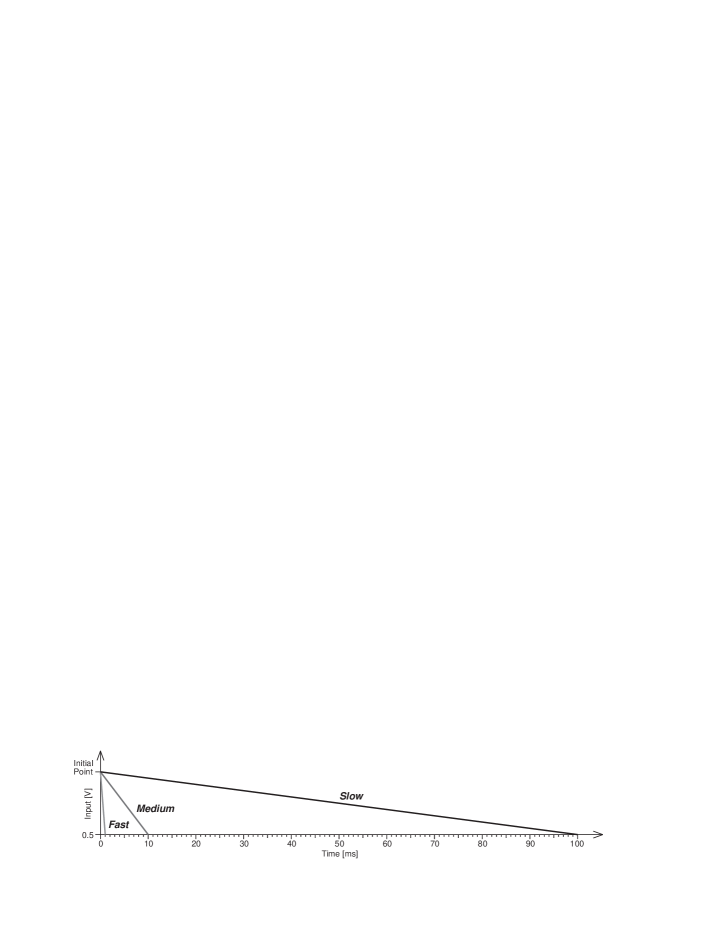
Figure 20: Three target trajectories with different speeds (time constants) employed in two types of the Constrained Association Modes.

5.2 Type #0 of Constrained Association Mode

Figure 21 shows the time-course of the network dynamics with a pair of a feedback path and an input port only in the internal space (Type #0 in Fig. 3) when a straight target trajectory is applied to the input port. The whole is divided into upper and lower blocks, which respectively show the Contractive and Expansive Cases. Each block has three rows, which are graphs depicted based on the simulation results with fast, medium, and slow speeds of the target trajectory from the top. The leftmost graphs show the target trajectories applied to the input port in the internal space. Their right graphs are the outputs in the internal space, and the next right ones depict the mapping relationship of Forward Subnet to increase intuitive understanding. The rightmost graphs are the outputs in the external space. In this figure, we selected five trajectories and depicted ten small subsidiary arrows at most on each of those trajectories at every particular period of time from the initial state to visually grasp their convergence speeds; the intervals among the small subsidiary arrows are $0.2{\sf ms}$, $2{\sf ms}$, and $20{\sf ms}$ from the top in each block. We omitted the Linear Case, since, as seen in the previous section, the outputs in the internal and external spaces are exactly the same and the trajectories are straight in this architecture of the Association Mode.

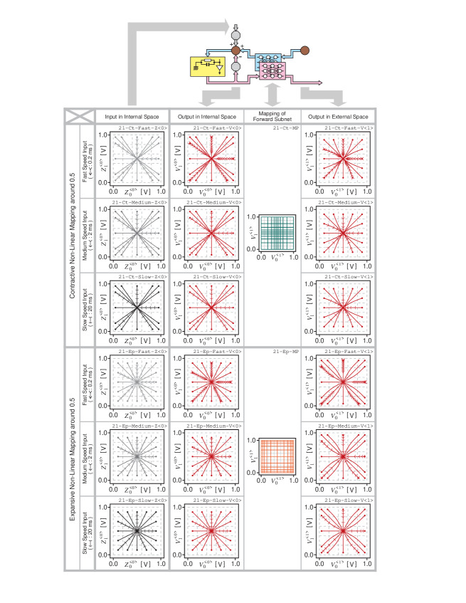
Figure 21: Simulation results for Type #0 of the Constrained Associative Mode in the two-dimensional model. In this experiment, a straight target trajectory instead of a goal point is applied to the input port existing only in the internal space. Network behavior for three different speeds of target trajectories is illustrated. The graphs only include the Contractive and Expansive Cases.

First, we consider the upper block for the Contractive Case. For a comparison with the experimental results stated later, the initial positions in the internal space are set to those farther from the center, in such a manner that the initial positions in the external space equal those in the internal space shown in Section 4. Since there is no signal through Backward Subnet in this case, the internal space’s output straightforwardly approaches the goal point, and an arbitrary point on the straight output trajectory in the internal space is mapped simply in a static way to that in the external space. 21-Ct-Fast-V<0> and 21-Ct-Fast-V<1> with fast speed inputs are basically the same as 18-Ct-V<0> and 18-Ct-V<1> in the previous section, although the similarity is somewhat obscure at a glance since the initial positions in both cases are different. Even if the speed of a target trajectory decreases, the fact remains that an arbitrary point on the straight output trajectory in the internal space is mapped statically to that in the external space. Comparisons of 21-Ct-Fast-V<1>, 21-Ct-Medium-V<1>, and 21-Ct-Slow-V<1> confirm that the output in the external space draws the same trajectory regardless of whether the target trajectory’s speed is fast or slow.

The Expansive Case is shown in the lower block. The initial positions in the internal space are set to the same ones as in Figs. 18 and 19 of Section 4. Also in this case, an arbitrary point on a straight output trajectory in the internal space is simply mapped in a static manner to that in the external space. 21-Ep-Fast-V<0> and 21-Ep-Fast-V<1> with fast speed inputs are the same as 18-Ep-V<0> and 18-Ep-V<1> in the Association Mode. As is clear from the comparison of 21-Ep-Fast-V<1>, 21-Ep-Medium-V<1>, and 21-Ep-Slow-V<1>, the output trajectories in the external space are almost the same regardless of whether the target trajectory’s speed is fast or slow. Note that the output curving in the upper block is opposite to that in the lower block; this fact is common to the results for Type #0 of the Association Mode.

5.3 Type #1 of Constrained Association Mode

Figure 22 shows the time-course of the network dynamics with a pair of a feedback path and an input port only in the external space (Type #1 in Fig. 3) when a straight target trajectory is applied to the input port. As in Fig. 21, three rows in the upper block mean the Contractive Case, and those in the lower block indicate the Expansive Case. The Linear Case was omitted for the same reason as in the previous subsection. The three rows in each block respectively denote the results with fast, medium, and slow speeds of the target trajectory from the top; these three speeds of the target trajectory are common to those in Fig. 21. The rightmost graphs are the target trajectories applied to the input port in the external space. The outputs in the internal and external spaces based on these inputs are shown in order from the left, placing the mapping relationship in Forward Subnet between them.

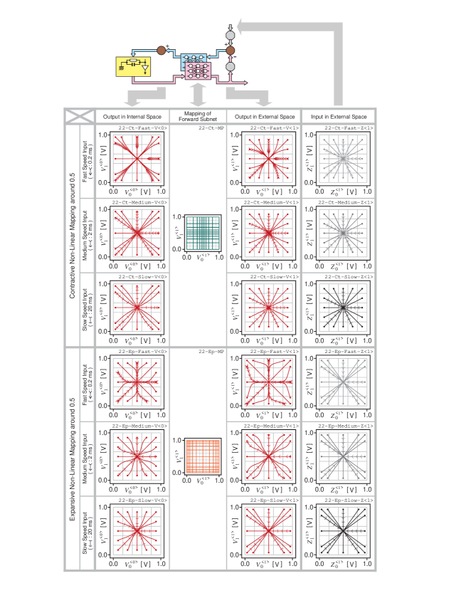
Figure 22: Simulation results for Type #1 of the Constrained Associative Mode in the two-dimensional model. In this experiment, a straight target trajectory instead of a goal point is applied to the input port existing only in the external space. Network behavior for three different speeds of target trajectories is depicted. The graphs also only include the Contractive and Expansive Cases.

First, we look at the Contractive Case in the upper block. The uppermost graphs 22-Ct-Fast-V<0> and 22-Ct-Fast-V<1> show basically the same responses as the uppermost graphs of Fig. 19 in the Association Mode 19-Ct-V<0> and 19-Ct-V<1>, although their initial positions are different. In both situations, large signals flow through Backward Subnet depending on the mapping relationship in Internetwork. Due to a detoured feedback loop via the external space, they affect both the internal and external spaces, where the output trajectories curve more greatly away from the straight. Those graphs with a fast target trajectory have characteristics common with the results in the Association Mode, but intriguingly, the graphs in the middle and lower rows show different tendencies from those in the upper row. By comparing 22-Ct-Medium-V<0> and 22-Ct-Medium-V<1> in the middle row with 22-Ct-Fast-V<0> and 22-Ct-Fast-V<1> in the upper row, the former curving for the trajectories in both the internal and external spaces is overall milder than the latter one. For the case with an even slower target trajectory shown in the lower row, the output in the external space 22-Ct-Slow-V<1> draws a straight line and nearly corresponds to the target trajectory 22-Ct-Slow-Z<1>. Instead, the output in the internal space $(V^{<0>}_{0},V^{<0>}_{1})$ draws a curved trajectory. Note that its curving direction is opposite to that with a fast target trajectory; it is obvious in comparison of 22-Ct-Slow-V<0> with 22-Ct-Fast-V<0>.

The relationship between Figs. 21 and 22 is also crucial. Compare the graphs in the lower row in the lower block of Fig. 21 with those in the lower row in the upper block of Fig. 22. Significantly, the output trajectories in the internal and external spaces are opposite to each other in these two cases with the slow target trajectories in Figs. 21 and 22 in such a manner that 21-Ep-Slow-V<0> and 22-Ct-Slow-V<1> are the same, as are 21-Ep-Slow-V<1> and 22-Ct-Slow-V<0>. Since the network dynamics are observed for a sufficiently long time and their results are plotted in Figs. 21 and 22, all of the output trajectories go to the goal point (the center). As predicted from the results in the one-dimensional model of the Assoiciation Mode, 17-Ct-V<0> and 17-Ct-V<1> of Fig. 17, the convergence speed near the center is very slow in the Contractive Case. For this reason, the intervals between small subsidiary arrows on a trajectory become dense in 22-Ct-Fast-V<0> or 22-Ct-Fast-V<1>, for instance. This phenomenon is caused regardless of the speed of a target trajectory applied to the input port, and so the convergence speed near the center is very slow even in 22-Ct-Slow-V<0> and 22-Ct-Slow-V<1>. Therefore, even though the convergence trajectories are identical, the periods required for converging to a goal point are not necessarily the same; this point is also a critical phenomenon that depends on the mapping relationship in Internetwork.

Next, we investigate the Expansive Case in the lower block. When a fast target trajectory is applied to the input port, as stated with respect to Fig. 19 in Type #1 of the Association Mode, large signals go through Backward Subnet depending on the mapping relationship in Internetwork. They affect both the internal and external spaces due to a detoured feedback loop via the external space, and the output trajectories curve greatly. By comparing 22-Ep-Fast-V<0> and 22-Ep-Fast-V<1> with 19-Ep-V<0> and 19-Ep-V<1> of Fig. 19 in the Association Mode, these pairs are almost the same. Those graphs with a fast target trajectory have characteristics common to the results in the Association Mode, but it is interesting that the graphs in the middle and lower rows indicate tendencies different from those in the upper row. In comparison of 22-Ep-Medium-V<0> and 22-Ep-Medium-V<1> in the middle row with 22-Ep-Fast-V<0> and 22-Ep-Fast-V<1> in the upper one, the former curving for the trajectories in both the internal and external spaces becomes milder than the latter one. Since this mapping relationship is expansive around the center but contractive at the edges near $0.0$ and $1.0$, we confirmed that the curving in a output trajectory is not monotonous but its tendency varies on the way to the center. For the case with an even slower target trajectory shown in the lower row, the output in the external space 22-Ep-Slow-V<1> draws a straight line and nearly corresponds to the target trajectory 22-Ep-Slow-Z<1> due to the function of the dynamical neurons in the internal space. Instead, the output in the internal space $V^{<0>}_{i}$ draws a curved trajectory, but its curving direction is opposite to that with a fast target trajectory; this observation is clear in the comparison of 22-Ep-Slow-V<0> with 22-Ep-Fast-V<0>.

Also in this case, we noticed an interesting relationship between Figs. 21 and 22. In a comparison of the graphs in the lower row in the upper block of Fig. 21 with those in the lower row in the lower block of Fig. 22, the output trajectories in the internal and external spaces are opposite to each other in the two cases with slow target trajectories of Figs. 21 and 22 in such a manner that 21-Ct-Slow-V<0> and 22-Ep-Slow-V<1> are the same, as are 21-Ct-Slow-V<1> and 22-Ep-Slow-V<0>.

5.4 On Inverse Mapping

For Type #0 of the Constrained Association Mode, the relationship between the output trajectories in the internal and external spaces is common regardless of whether a fast or a slow target trajectory is applied to the input port. A straight target trajectory in the internal space was transformed based on the mapping relationship already acquired in Internetwork, and its warped trajectory simply appeared in the external space as a statically mapped path. In contrast, for Type #1 of the Constrained Association Mode, a different appearance was presented. When a fast target trajectory was applied to the input port, the output trajectories in both the internal and external spaces are determined to emphasize their curving tendency due to a detoured feedback loop via the external space.

When, in Type #1 architecture, a very slow target trajectory from an initial point to a goal point is applied to the input port in the external space, conversely, the output in the external space completely follows its target trajectory; no signal flows through Backward Subnet. If the mapping relationship from the internal space to the external space by Forward Subnet is now assumed to be $M$, an output trajectory, which was converted from that in the external space by the “inverse” mapping relationship $M^{-1}$, appears in the internal space in such a manner that the output in the external space transmitted by Forward Subnet simply becomes a straight target trajectory that is applied to the input port in the external space. The following are specific examples: The mapping from the output in the internal space 21-Ct-Slow-V<0> to that in the external space 21-Ct-Slow-V<1> in the Contractive Case for Type #0 of the Constrained Association Mode is the same as the mapping from that in the external space 22-Ep-Slow-V<1> to that in the internal space 22-Ep-Slow-V<0> in the Expansive Case for Type #1 of the Constrained Association Mode. In addition, the mapping from the output in the internal space 21-Ep-Slow-V<0> to that in the external space 21-Ep-Slow-V<1> in the Expansive Case for Type #0 of the Constrained Association Mode is the same as the mapping from that in the external space 22-Ct-Slow-V<1> to that in the internal space 22-Ct-Slow-V<0> in the Contractive Case for Type #1 of the Constrained Association Mode.

Thus, when an extremely slow target trajectory is applied to the input port in the external space on Type #1 of the Constrained Association Mode, an output trajectory, which was converted from the output in the external space by the inverse mapping $M^{-1}$, appears in the internal space, although only the mapper from the internal space to the external space $M$ does exist but the one for the inverse mapping $M^{-1}$ does not exist inside the whole network.

6 Conclusions

In this paper, we propose a hierarchically modular neural network model composed of two types of neurons with different time constants (one is dynamic and the other is regarded as static), and precisely examined its dynamical behavior through simulation studies. We summarize our results in the following.

$\diamondsuit$ Model Proposal

• Supposing that the outputs of dynamical neurons are transformed to other output variables by a mapping function or a multi-layered neural network with static neurons, we designed an energy function consisting of those output variables. A concrete network of our proposed model can be derived based on the process that minimizes its energy function.

• Our network has a ladder-shaped architecture with internal and external spaces, each of which has a pair of a feedback path and an input port.

• Some groups of synaptic connections exist in the whole network. Among them, only those in layered networks with static neurons have plasticity. All other connections are fixed.

• Two kinds of dynamics, activity dynamics for dynamical neurons and learning dynamics for synaptic connections in a layered network, progress simultaneously, and both cooperatively determine the network’s total behavior.

• We considered our dynamical neural network a model and supposed two modes, Learning and Association (Types #0 or #1), which depend on whether a pair of a feedback path and an input port is in the internal or external space or in both. In either mode, the total dynamics are produced due to the cooperation between dynamic and static neurons.

$\diamondsuit$ Learning Mode

• When appropriate sinusoidal and/or quasi-sinusoidal waves are applied in the Learning Mode from the outside of the model to the input ports, the network can automatically acquire the corresponding mapping relationship in Internetwork connecting the internal space with the external space. The sinusoidal signal here corresponds to repetitive neuronal bursting, which represents a periodic wave in the short-term average density of nerve impulses or in the membrane potential.

• When the given periodic signals have different waveforms, a non-linear mapping relationship (instead of a linear one) is formed in Internetwork, depending on the shapes of the waves.

• The model can be expanded to a two-dimensional scheme. When sinusoidal waves with adequately different frequencies are applied to the input ports, a two-dimensional mapping relationship can be acquired in Internetwork based on its generalization capability.

• Such a situation is recommended where the frequencies of these two sinusoidal waves are either only slightly different or extremely different; this aspect is coincident with the framework of Lissajous curves.

• When periodic signals with different waveforms are applied to the internal and external spaces, non-linear mapping relationships can be acquired in Internetwork even in a two-dimensional model.

• In the Learning Mode, we can confirm some interesting phenomena in which two kinds of dynamics, that is, activity dynamics due to dynamical neurons and learning dynamics in a layered network with static neurons, seem to be cooperatively related.

$\diamondsuit$ Association Mode

• In the Association Mode, we found that the speed of convergence from an initial point to a goal point varies depending on how the mapping relationship between the internal and external spaces is warped. In the two-dimensional model, we confirmed that a convergence trajectory can become out of the straight due to the warping of the mapping relationship.

• In Type #1 of the Association Mode with a pair of a feedback path and an input port only in the external space, we clarified that a convergence trajectory curves more greatly compared with Type #0 of the Association Mode with a pair of a feedback path and an input port only in the internal space.

• If Internetwork were trained to be linear through its full range, the dynamics for the internal and external spaces in both Type #0 and Type #1 of the Association Mode would be identical to those of the original Hopfield model.

• Although we introduced the Association Mode in Section 4 and the Constrained Association Mode in Section 5, it is also reasonable to call the former the “Unconstrained” Association Mode.

$\diamondsuit$ Inverse Mapping

• In Type #0 of the Constrained Association Mode, no signal propagates through Backward Subnet in principle. Applying a very slow target trajectory (instead of a goal point) to the input port in Type #1 of the Constrained Association Mode, signals flowing through Backward Subnet become quite small due to the function of the dynamical neurons in the internal space. Hence, in both architectures of the Constrained Association Mode with an extremely slow target trajectory, curving for the output trajectories in the internal and external spaces is generated only by the static mapping relationship of Internetwork.

• In Type #1 of the Constrained Association Mode with a pair of a feedback path and an input port only in the external space, if $M$ is the mapping relationship of Forward Subnet, a phenomenon appears in such a manner that a mapper with $M^{-1}$ does exist, although it does not exist explicitly in the whole network. In other words, an output trajectory is generated in the internal space, that is transformed by a mapper with $M^{-1}$ from a target trajectory applied in the external space.

Although the Learning Mode and the two kinds of Association Modes (Unconstrained / Constrained) were artificially classified on the basis of their structural differences and the ON/OFF operation of the learning dynamics given by Eq. (29) was consistently selected here, it might be possible to construct a model in which such modes can be switched automatically according to the situation and the form of the input signals given from the outside. In the Learning Mode discussed in Section 3, a non-distorted sinusoidal wave was applied to the input port in the internal space, but the waveform is not limited to such a case. For the two-dimensional model, the two inputs for the horizontal and vertical axes have no correlation, but it is quite significant to examine various cases in which the two inputs are correlated. This paper refers only to one-dimensional and two-dimensional models. After increasing the dimension from one to two, it should be straightforward to expand it to three and higher. Also, we only treated convergent dynamics toward a fixed point throughout our paper, but we can discuss divergent dynamics by changing the signs of the terms in the energy function [55][62][63]. These expansions will be developed in future work.

Even though, as suggested previously, our primary motivation is not the solution of any practival problems, we expect that our framework, with a dynamical system relaxing in a warped space, has the potential to several practical applications. Examples are advanced associative memory tasks, optimization problems, or control issues in which each constraint must be minimized in the corresponding non-linear subspace. If the mapping relationship of Internetwork is chosen appropriately, it may be possible to expand the basins of attraction in a warped space. Our model then might improve the performance of associative recall and enhance the memory capacity when applying it to an associative memory task [5]. In those cases, as discussed in detail in Section 5, it is crucial to provide an adequate constraint in the form of input signals from the outside to the model in order to control the convergent or divergent trajectory in the internal space as intended. In this paper, we mainly discussed depth-wise or vertical (hierarchical) modularity, but not spread-wise or horizontal modularity as in internetworking. This point is significant not only from an architectural viewpoint but also in the sense of illustrating the performance of our proposed model. Our approach opens a large array of subjects. In future work, we plan to discuss a general model that is not limited to internal and external spaces but contains multiple subspaces.

Acknowledgements: This work was supported in part by Ryukoku University Fund for Overseas Research, Office of Naval Research Grant N00014-22-1-2699, and National Science Foundation grant 1835202.

References

- [1] Aihara, K., and Ichinose, N. Modeling and complexity in neural networks. Artificial Life and Robotics 3 (1999), 148–154.
- [2] Amari, S.-I. Theory of adaptive pattern classifiers. IEEE Transactions on Electronic Computers 16 (1967), 299–307.
- [3] Amari, S.-I. Neural theory of association and concept-formation. Biological Cybernetics 26 (1977), 175–185.
- [4] Block, H. D. The perceptron: A model for brain functioning. I. Reviews of Modern Physics 34 (1962), 123–135.
- [5] Cabrera, E., and Sossa, H. Generating exponentially stable states for a Hopfield Neural Network. Neurocomputing 275 (2018), 358–365.
- [6] Carpenter, G. A., Cohen, M. A., Grossberg, S.; Kohonen, T., Oja, E.; Palm, G. H. J. J., and Tank, D. W. Technical comments: computing with neural networks. Science 235 (1987), 1226–1229.
- [7] Doya, K. Metalearning and neuromodulation. Neural Networks 15 (2002), 495–506.
- [8] FitzHugh, R. Mathematical models of threshold phenomena in the nerve membrane. Bulletin of Mathematical Biophysics 17 (1955), 257–278.
- [9] Flexner, A., and Dijkgraaf, R. The usefulness of useless knowledge. Princeton University Press, 2017.
- [10] Fukushima, K. Congnitron: A self-organizing multilayered neural network. Biological Cybernetics 20 (1975), 121–136.
- [11] Fukushima, K. Neocognitron: A self-organizing neural network model for a mechanism of pattern recognition unaffected by shift in position. Biological Cybernetics 36 (1980), 193–202.
- [12] Fukushima, K. A neural network model for selective attention in visual pattern recognition. Biological Cybernetics 55 (1986), 5–15.
- [13] Fukushima, K. Artificial vision by multi-layered neural networks: Neocognitron and its advances. Neural Networks 37 (2013), 103–119.
- [14] Fukushima, K., Miyake, S., and Ito, T. Neocognitron: A neural network model for a mechanism of visual pattern recognition. IEEE Transactions on Systems, Man, and Cybernetics 13 (1983), 826–834.
- [15] Grossberg, S. Adaptive pattern classification and universal recoding: I. parallel development and coding of neural feature detectors. Biological Cybernetics 23 (1976), 121–134.
- [16] Grossberg, S. Adaptive resonance theory: How a brain learns to consciouly attend, learn, and recognize a changing world. Neural Networks 37 (2013), 1–47.
- [17] Hafner, D., Irpan, A., Davidson, J., and Heess, N. Learning hierarchical information flow with recurrent neural modules. In Advances in Neural Information Processing Systems (NIPS) (2017), vol. 30.
- [18] Hebb, D. O. The organization of behavior. New York: Wiley, 1949.
- [19] Hecht-Nielsen, R. Counterpropagation networks. In Proc. IEEE First International Conference on Neural Networks (1987), vol. 2, pp. 19–32.
- [20] Hect-Nielsen, R. Neurocomputing: Picking the human brain. IEEE Spectrum (March 1988), 36–41.
- [21] Hinton, G. E., Osindero, S., and Teh, Y. A fast learning algorithm for deep belief nets. Neural Computation 18 (2006), 1527–1554.
- [22] Hinton, J., and Salakhutdinov, R. R. Reducing the dimensionality of data with neural networks. Science 313 (2006), 504–507.
- [23] Hodgkin, A. L., and Huxley, A. F. A quantitative description of membrane current and its application to conduction and excitation in nerve. The Journal of Physiology 117 (1952), 500–544.
- [24] Hopfield, J. J. Neural networks and physical systems with emergent collective computational abilities. In Proc. the National Academy of Sciences, U.S.A. (1982), vol. 79, pp. 2554–2558.
- [25] Hopfield, J. J. Neurons with graded response have collective computational properties like those of two-state neurons. In Proc. the National Academy of Science, U.S.A. (1984), vol. 81, pp. 3088–3092.
- [26] Hopfield, J. J., and Tank, D. W. “neural” computation of decisions in optimization problems. Biological Cybernetics 52 (1985), 141–152.
- [27] Hubel, D. H., and Wiesel, T. N. Receptive fields of single neurones in the cat’s striate cortex. The Journal of Physiology 148 (1959), 574–591.
- [28] Kohonen, T. Correlation matrix memories. IEEE Transactions on Computers C-21 (1972), 353–359.
- [29] Kohonen, T. Self-organized formation of topologically correct feature maps. Biological Cybernetics 43 (1982), 59–69.
- [30] Kosko, B. Bidirectional associative memories. IEEE Transactions on Systems, Man, and Cybernetics 18 (1988), 49–60.
- [31] Markoff, J. How many computers to identify cat? 16,000. The New York Times, June 2012.
- [32] Matsuoka, K. Sustained oscillations generated by mutually inhibiting neurons with adaptation. Biological Cybernetics 52 (1985), 367–376.
- [33] McCulloch, W. S., and Pitts, W. A logical calculus of the ideas immanent in nervous activity. Bulletin of Mathematical Biophysics 5 (1943), 115–133.
- [34] Meunier, D., Lambiotte, R., and Bullmore, E. T. Modular and hierarchically modular organization of brain networks. Frontiers in Neuroscience 4, Art.200 (2010).
- [35] Millman, D., Mihalas, S., Kirkwood, A., and Niebur, E. Self-organized criticality occurs in non-conservative neuronal networks during ‘up’ states. Nature Physics 6 (2010), 801–805.
- [36] Minsky, M., and Papert, S. Perceptrons. The MIT Press, Cambridge, MA, U.S.A., 1969.
- [37] Morishita, I., and Yajima, A. Analysis and simulation of networks of mutually inhibiting neurons. Kybernetik 11 (1972), 154–165.
- [38] Nagumo, J., Arimoto, S., and Yoshizawa, S. An active pulse transmission line simulating nerve axon. In Proc. IRE (1962), vol. 50, pp. 2061–2070.
- [39] Nakano, K. Associatron - a model of associative memory. IEEE Transactions on Systems, Man, and Cybernetics 2 (1972), 380–388.
- [40] Nicolini, C., and Bifone, A. Modular structure of brain functional networks: breaking the resolution limit by surprise. Scientific Reports 6, Art.19250 (2016).
- [41] Niebur, E., and Erdos, P. Computer simulation of networks of electrotonic neurons. In Computer simulation in brain science, R. M. J. Cotterill, Ed. Cambridge University Press, Cambridge, UK, 1988, pp. 148–163.
- [42] Ozawa, S., Roy, A., and Roussinov, D. A multitask learning model for online pattern recognition. IEEE Transactions on Neural Networks 20 (2009), 430–445.
- [43] Ozawa, S., Tsutsumi, K., and Baba, N. An artificial modular neural network and its basic dynamical characteristics. Biological Cybernetics 78 (1998), 19–36.
- [44] Plenz, D., and Niebur, E. Criticality in neural systems. Wiley VCH, 2014.
- [45] Rosenblatt, F. The perceptron: A probabilistic model for information storage and organization in the brain. Psychological Review 65 (1958), 386–408.
- [46] Rumelhart, D. E., Hinton, G. E., and Williams, R. J. Learning internal representation by error propagation. In Parallel distributed processing: Explorations in the microstructures of cognition, D. E. Rumelhart and J. L. McClelland, Eds., vol. 1. The MIT Press, Cambridge, MA, U.S.A., 1986, pp. 318–362.
- [47] Rumelhart, D. E., Hinton, G. E., and Williams, R. J. Learning representations by back-propogating errors. Nature 323 (1986), 533–536.
- [48] Steinbuch, K., and Piske, U. A. W. Learning matrices and their applications. IEEE Transactions on Electronic Computers 12 (1963), 846–862.
- [49] Tank, D. W., and Hopfield, J. J. Simple ‘neural’ optimization networks: An A/D converter, signal decision circuit, and a linear programming circuit. IEEE Transactions on Circuit and Systems 33 (1986), 533–541.
- [50] Tsujita, K., Tsuchiya, K., and Onat, A. Decentralized autonomous control of a quadruped locomotion robot. Artificial Life and Robotics 5 (2003), 152–158.
- [51] Tsutsumi, K. Neural control of 3-dimentional truss structure. Neural Networks 1, Supl. 1 (1988), 364.
- [52] Tsutsumi, K. A multi-layered neural network composed of back-prop. and Hopfield nets and internal space representation. In Proc. International Joint Conference on Neural Networks (1989), pp. 365–371.
- [53] Tsutsumi, K. Cross-Coupled Hopfield Nets via generalized-delta-rule-based internetworks. In Proc. International Joint Conference on Neural Networks (1990), vol. 2, pp. 259–265.
- [54] Tsutsumi, K. Higher degree error backpropagation in cross-coupled Hopfield nets. In Proc. International Joint Conference on Neural Networks (1991), vol. 2, pp. 349–355.
- [55] Tsutsumi, K. On redundancy in neural architecture: dynamics of a simple module-based neural network and initial-state independence. Neural Networks 12 (1999), 1075–1085.
- [56] Tsutsumi, K. Relaxing in a warped space: An effect due to the cooperation of static and dynamical neurons. In Proc. International Joint Conference on Neural Networks (2003), pp. 897–901.
- [57] Tsutsumi, K., Katayama, K., and Matsumoto, H. Neural computation for controlling the configuration of 2-dimentional truss structure. In Proc. the IEEE Annual International Conference on Neural Networks (1988), pp. 575–586.
- [58] Tsutsumi, K., and Matsumoto, H. Ring neural network qua a generator of rhythmic oscillation with period control mechanism. Biological Cybernetics 51 (1984), 181–194.
- [59] Tsutsumi, K., and Matsumoto, H. A synaptic modification algorithm in consideration of the generation of rhythmic oscillation in a ring neural network. Biological Cybernetics 50 (1984), 419–430.
- [60] Tsutsumi, K., and Matsumoto, H. Neural computation and learning strategy for manipulator position control. In Proc. the IEEE First Annual International Conference on Neural Networks (1987), vol. 4, pp. 525–534.
- [61] Tsutsumi, K., and Matsumoto, H. A synaptic modification algorithm and rhythmic oscillation. In Computer simulation in brain science, R. M. J. Cotterill, Ed. Cambridge University Press, Cambridge, UK, 1988, pp. 268–292.
- [62] Tsutsumi, K., and Nakajima, K. Maximum/minimum detection by a module-based neural network with redundant architecture. In Proc. International Joint Conference on Neural Networks (1999), p. 792: Session: 3.4.
- [63] Tsutsumi, K., and Nakajima, K. Dynamics and local minima of a simple neural network for optimization. In Proc. International Joint Conference on Neural Networks (2001), pp. 353–358.
- [64] Werbos, P. J. Beyond regression: New tools for prediction and analysis in the behavioral sciences. PhD thesis, Harvard University, 1974.
- [65] Widrow, B., and Hoff, M. E. Adaptive switching circuits. In IRE WESCON Convention Record (1960), pp. 96–104.
- [66] Williams, R. J., and Zipser, D. Gradient-based learning algorithms for recurrent connectionist networks. Tech. Rep. Tech. Rep. NU-CCS-90-9, College of Computer Science, Northeastern University, Boston, MA, U.S.A., 1990.
- [67] Williams, R. J., and Zipser, D. Gradient-based learning algorithms for recurrent networks and their computational complexity. In Back-propagation: theory, architectures and applications, Y. Chauvin and D. E. Rumelhart, Eds. L. Erlbaum Associates Inc., Hillsdale, NJ, U.S.A., 1995, pp. 433–486.