Instance-specific and Model-adaptive Supervision for
Semi-supervised Semantic Segmentation

Abstract

Recently, semi-supervised semantic segmentation has achieved promising performance with a small fraction of labeled data. However, most existing studies treat all unlabeled data equally and barely consider the differences and training difficulties among unlabeled instances. Differentiating unlabeled instances can promote instance-specific supervision to adapt to the model’s evolution dynamically. In this paper, we emphasize the cruciality of instance differences and propose an instance-specific and model-adaptive supervision for semi-supervised semantic segmentation, named iMAS. Relying on the model’s performance, iMAS employs a class-weighted symmetric intersection-over-union to evaluate quantitative hardness of each unlabeled instance and supervises the training on unlabeled data in a model-adaptive manner. Specifically, iMAS learns from unlabeled instances progressively by weighing their corresponding consistency losses based on the evaluated hardness. Besides, iMAS dynamically adjusts the augmentation for each instance such that the distortion degree of augmented instances is adapted to the model’s generalization capability across the training course. Not integrating additional losses and training procedures, iMAS can obtain remarkable performance gains against current state-of-the-art approaches on segmentation benchmarks under different semi-supervised partition protocols.

1 Introduction

Though semantic segmentation studies [27, 6] have achieved significant progress, their enormous success relies on large datasets with high-quality pixel-level annotations. Semi-supervised semantic segmentation (SSS) [19, 29] has been proposed as a powerful solution to mitigate the requirement for labeled data. Recent research on SSS has two main branches, including the self-training (ST) [25] and consistency regularization (CR) [39] based approaches. [45] follows a self-training paradigm and performs a selective re-training scheme to train on labeled and unlabeled data alternatively. Differently, CR-based works [33, 26] tend to apply data or model perturbations and enforce the prediction consistency between two differently-perturbed views for unlabeled data. In both branches, recent research [12, 46, 18] demonstrates that strong data perturbations like CutMix can significantly benefit the SSS training. To further improve the SSS performance, current state-of-the-art approaches [1, 41] integrate the advanced contrastive learning techniques into the CR-based approaches to exploit the unlabeled data more efficiently. Works in [20, 23] also aim to rectify the pseudo-labels through training an additional correcting network.

Despite their promising performance, SSS studies along this line come at the cost of introducing extra network components or additional training procedures. In addition, majorities of them treat unlabeled data equally and completely ignore the differences and learning difficulties among unlabeled samples. For instance, randomly and indiscriminately perturbing unlabeled data can inevitably over-perturb some difficult-to-train instances. Such over-perturbations exceed the generalization capability of the model and hinder effective learning from unlabeled data. As discussed in [46], it may also hurt the data distribution. Moreover, in most SSS studies, final consistency losses on different unlabeled instances are minimized in an average manner. However, blindly averaging can implicitly emphasize some difficult-to-train instances and result in model overfitting to noisy supervision.

In this paper, we emphasize the cruciality of instance differences and aim to provide instance-specific supervision on unlabeled data in a model-adaptive way. There naturally exists two main questions. First, how can we differentiate unlabeled samples? We design an instantaneous instance “hardness,” to estimate 1) the current generalization ability of the model and 2) the current training difficulties of distinct unlabeled samples. Its evaluation is closely related to the training status of the model, e.g., a difficult-to-train sample can become easier with the evolution of the model. Second, how can we inject such discriminative information into the SSS procedure? Since the hardness is assessed based on the model’s performance, we can leverage such information to adjust the two critical operations in SSS, i.e., data perturbations and unsupervised loss evaluations, to adapt to the training state of the model dynamically.

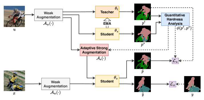
Figure 1: Diagram of our proposed iMAS. In a teacher-student framework, labeled data $(x,y)$ is used to train the student model, parameterized by $\theta_{s}$, by minimizing the supervised loss $\mathcal{L}_{x}$. Unlabeled data $u$, weakly augmented by $\mathcal{A}_{w}(\cdot)$, is first fed into both the student and teacher models to obtain predictions $p^{s}$ and $p^{t}$, respectively. Then we perform quantitative hardness evaluation on each unlabeled instance by strategy $\phi(p^{t},p^{s})$. Such hardness information can be subsequently utilized: 1) to apply an adaptive augmentation, denoted by $\mathcal{A}_{s}(\cdot)$, on unlabeled data to obtain the student model’s prediction $\hat{p}$; 2) to weigh the unsupervised loss $\mathcal{L}_{u}$ in a instance-specific manner. The teacher model’s weight, $\theta_{t}$, is updated by the exponential moving average (EMA) of $\theta_{s}$ across the training course.

Motivated by all these observations, we propose an instance-specific and model-adaptive supervision, named iMAS, for semi-supervised semantic segmentation. As shown in Figure 1, following a standard consistency regularization framework, iMAS jointly trains the student and teacher models in a mutually-beneficial manner. The teacher model is an ensemble of historical student models and generates stable pseudo-labels for unlabeled data. Inspired by empirical and mathematical analysis in [14, 40], difficult-to-train instances may undergo considerable disagreement between predictions of the EMA teacher and the current student. Thus in iMAS, we first evaluate the instance hardness of each unlabeled sample by calculating the class-weighted symmetric intersection-over-union (IoU) between the segmentation predictions of the teacher (the historical) and student (the most recent) models. Then based on the evaluation, we perform model-adaptive data perturbations on each unlabeled instance and minimize an instance-specific weighted consistency loss to train models in a curriculum-like manner. In this way, different unlabeled instances are perturbed and weighted in a dynamic fashion, which can better adapt to the model’s generalization capability throughout the training processes.

Benefiting from this instance-specific and model-adaptive design, iMAS obtains state-of-the-art (SOTA) performance on Pascal VOC 2012 and Cityscapes datasets under different partition protocols. For example, our method obtains a high mIOU of 75.3% with only 183 labeled data on VOC 2012, which is 17.8% higher than the supervised baseline and 4.3% higher than the previous SOTA. Our main contributions are summarized as follows,

• iMAS can boost the SSS performance by highlighting the instance differences, without introducing extra network components or training losses.

• We perform a quantitative hardness-evaluating analysis for unlabeled instances in segmentation tasks, based on the class-weighted teacher-student symmetric IoU.

• We propose an instance-specific and model-adaptive SSS framework that injects instance hardness into loss evaluation and data perturbation to dynamically adapt to the model’s evolution.

2 Related work

Recent studies on CR-based semi-supervised learning have achieved impressive improvements in classification tasks [32]. Based on clustering assumptions, these methods enforce prediction consistency on the unlabeled sample with different perturbations. Early works like Mean-Teacher [39] aimed to generate a more robust and accurate pseudo-label using ensemble techniques. VAT [30], UDA [43], and MixMatch [4] then improved the performance by using more advanced augmentations, like adversarial perturbations [13], randomAug [9, 31], and Mixup [49]. FixMath [37] inherited the idea of strong augmentations and further boosted the accuracy by a fixed threshold to select confident pseudo-labels. More recent research intended to introduce additional training and supervision, like using contrastive learning [51, 44], distribution alignment [3, 50], and Sinkhorn-Knopp clustering [38], to further enhance the performance.

Motivated by the progress in semi-supervised classification, some studies aim to achieve dense segmentation performance with only a fraction of labels. Generally, recent jobs can be categorized into two main groups. 1) rectifying the pseudo-labels by training extra correcting networks [20, 28, 23], re-balancing the classes [17], or using multiple predictions [26]; 2) exploring more supervisions by using extra losses [7], utilizing stronger augmentations [45, 46], or applying the advanced contrastive learning [41, 52, 1, 54]. These studies show promising results at the cost of integrating extra network components or additional training processes. To the best of our knowledge, all the existing studies indiscriminately perturb unlabeled samples and minimize an average consistency loss over all unlabeled samples. Differently, we differentiate different samples in terms of the learning difficulty, evaluated as instance hardness. We utilize the hardness to guide the training process and achieve new SOTA performance on several semi-supervised semantic segmentation benchmarks.

Instance hardness [36, 34, 35, 5] has been widely studied in hard example mining [47] and curriculum learning [53]. Their evaluation mainly depends on the instantaneous or historical training losses with respect to ground truths. Lacking accurate label information makes hardness measurements of unlabeled instances much more challenging. Some works [47, 21, 42] perform hardness analysis on unlabeled data to split all the samples into the hard and easy groups by sorting or ranking the hardness with a predefined threshold. Such methods only require qualitative analysis for selecting or filtering purposes. However, specific quantitative hardness analysis, especially on segmentation tasks, is still under-explored. In iMAS, we need the quantitative hardness to determine the mixup between strongly and weakly augmented crops, as well as the exact unsupervised loss weight for each unlabeled instance. Thus we propose a new class-weighted symmetric metric to evaluate the hardness of unlabeled instances in segmentation tasks.

3 Method

The goal of semi-supervised semantic segmentation is to generalize a segmentation model by effectively leveraging a labeled training set $D_{x}=\{(x_{i},y_{i})\}_{i=1}^{|D_{x}|}$ and a large unlabeled training set $D_{u}=\{u_{i}\}_{i=1}^{|D_{u}|}$, with typically $|D_{x}|\ll|D_{u}|$. In our method, following the consistency regularization (CR) based semi-supervised classification approaches [37, 43], we aim to train the segmentation encoder and decoder on both labeled and unlabeled data simultaneously. In each iteration, given a batch of labeled samples $\mathcal{B}_{x}=\{(x_{i},y_{i})\}_{i=1}^{|\mathcal{B}_{x}|}$ and unlabeled samples $\mathcal{B}_{u}=\{u_{i}\}_{i=1}^{|\mathcal{B}_{u}|}$, the overall training loss is formulated as,

$$\mathcal{L}=\mathcal{L}_{x}+\lambda_{u}\mathcal{L}_{u},$$ (1)

where $\lambda_{u}$ is a scalar hyper-parameter to adjust the relative importance between the supervised loss $\mathcal{L}_{x}$ on $\mathcal{B}_{x}$ and the unsupervised loss $\mathcal{L}_{u}$ on $\mathcal{B}_{u}$. Without introducing extra losses or network components, iMAS can perform effectively quantitative hardness analysis for each unlabeled instance and then supervise the training on unlabeled data in a model-adaptive fashion across the training course. In this section, we first introduce our proposed iMAS at a high level in Sec. 3.1 and then present the detailed designs in terms of the quantitative hardness analysis in Sec. 3.2 and the model-adaptive guidance in Sec. 3.3.

Algorithm 1 iMAS algorithm in a mini-batch.

Input: Labeled batch $\mathcal{B}_{x}=\{(x_{i},y_{i})\}_{i=1}^{|\mathcal{B}_{x}|}$, unlabeled batch $\mathcal{B}_{u}=\{u_{i}\}_{i=1}^{|\mathcal{B}_{u}|}$ ($|\mathcal{B}_{x}|=|\mathcal{B}_{u}|$), hardness evaluation strategy $\phi$, weak augmentation $\mathcal{A}_{w}(\cdot)$, adaptive strong augmentation $\mathcal{A}_{s}(\cdot)$
Parameter: confidence threshold $\tau$, unsupervised loss weight $\lambda_{u}$

1:  $\mathcal{L}_{x}=\frac{1}{|\mathcal{B}_{x}|}\sum_{i=1}^{|\mathcal{B}_{x}|}\frac{1}{H\times W}\sum_{j=1}^{H\times W}\mathrm{H}(\hat{y}_{i}(j),y_{i}(j))$  // calculate the supervised loss.

2:  for $u_{i}\in\mathcal{B}_{u}$ do

3:     $p^{s}_{i}=f_{\theta_{s}}(\mathcal{A}_{w}(u_{i}))$  // obtain segmentation predictions on weakly-augmented instances.

4:     $p^{t}_{i}=f_{\theta_{t}}(\mathcal{A}_{w}(u_{i}))$  // obtain pseudo-labels from the teacher model.

5:     $\gamma_{i}=\phi(p^{t}_{i},p^{s}_{i})$  // evaluate the hardness of each instance.

6:  end for

7:  $\mathcal{L}_{u}=\frac{1}{|\mathcal{B}_{u}|}\sum_{i=1}^{|\mathcal{B}_{u}|}\frac{\gamma_{i}}{2H\times W}\sum_{j=1}^{H\times W}[\mathbbm{1}(\max(p^{t}_{i}(j))\geq\tau)\mathrm{H}(f_{\theta_{s}}(\mathcal{A}_{s}^{I}(u_{i})),p^{t}_{i}(j))+$   $\mathbbm{1}(\max(p^{t^{\prime}}_{i}(j))\geq\tau)\mathrm{H}(f_{\theta_{s}}(\mathcal{A}_{s}^{C}(u_{i})),p^{t^{\prime}}_{i}(j))]$  // calculate model-adaptive consistency loss

8:  return  $\mathcal{L}=\mathcal{L}_{x}+\lambda_{u}\mathcal{L}_{u}$

3.1 Overview

Built on top of the CR-based semi-supervised framework, iMAS jointly trains a student model with learnable weights $\theta_{s}$ and a teacher model with learnable weights $\theta_{t}$ in a mutually-beneficial manner. The complete algorithm is shown in algorithm 1. On the one hand, the teacher model is updated by the exponential moving averaging of the student weights, i.e.,

$$\theta_{t}\leftarrow\alpha\theta_{t}+(1-\alpha)\theta_{s},$$ (2)

where $\alpha$ is a common momentum parameter, set as 0.996 by default. On the other hand, the student model relies on the pseudo-labels generated by the teacher model to be trained on the unlabeled data. Specifically, the student model is trained via minimizing the total loss $\mathcal{L}$ in Equation 1, which consists of two cross-entropy loss terms, $\mathcal{L}_{u}$ and $\mathcal{L}_{x}$, applied on labeled and unlabeled data, respectively. Let $\mathrm{H}(z_{1},z_{2})$ denote the cross-entropy loss between prediction distributions $z_{1}$ and $z_{2}$. The supervised loss $\mathcal{L}_{x}$ is calculated as,

$$\mathcal{L}_{x}=\frac{1}{|\mathcal{B}_{x}|}\sum_{i=1}^{|\mathcal{B}_{x}|}\frac{1}{H\times W}\sum_{j=1}^{H\times W}\mathrm{H}(\hat{y}_{i}(j),y_{i}(j)),$$ (3)

where $\hat{y}_{i}=f_{\theta_{s}}(\mathcal{A}_{w}(x_{i}))$, represents the segmentation result of the student model on the $i$-th weakly-augmented labeled instance. $j$ represents the $j$-th pixel on the image or the corresponding segmentation mask with a resolution of $H\times W$. The weak augmentation $\mathcal{A}_{w}$ includes standard resizing, cropping, and flipping operations. Importantly, the way to leverage the unlabeled data is the key to semi-supervised learning and also the crucial part differentiating our method from others. In most CR-based studies, the standard (${std}$) unsupervised loss $\mathcal{L}_{u}^{std}$ is simply,

$$\mathcal{L}_{u}^{std}\!=\!\frac{1}{|\mathcal{B}_{u}|}\!\sum_{i=1}^{|\mathcal{B}_{u}|}\!\frac{1}{H\times W}\sum_{j=1}^{H\times W}\!\mathbbm{1}(\max(p^{t}_{i}(j))\!\geq\!\tau)\!\mathrm{H}(\hat{p}_{i}(j),\!p^{t}_{i}(j)),$$ (4)

where $\hat{p}_{i}=f_{\theta_{s}}(\mathcal{A}_{s}^{std}(u_{i}))$ represents the segmentation output of the student model on the $i$-th unlabeled instance augmented by $\mathcal{A}_{s}^{std}$, while $p^{t}_{i}=f_{\theta_{t}}(\mathcal{A}_{w}(u_{i}))$ represents the segmentation outputs of the teacher model on the $i$-th weakly-augmented unlabeled instance. $\tau$ is a predefined confidence threshold to select high-confidence predictions. $\mathcal{A}_{s}^{std}$ represents standard instance-agnostic strong augmentations, including intensity-based data augmentations [9] and CutMix [48] as shown in Table 1. However, such operations are limited in ignoring the differences and learning difficulties among unlabeled samples.

Differently, in our iMAS, we treat each instance discriminatively and provide instance-specific supervision on the training of unlabeled data. As shown in Figure 1, we first evaluate the hardness of each weakly-augmented unlabeled instance via strategy $\phi$, and then employ the instance-specific and model-adaptive supervision on the strong augmentations $\mathcal{A}_{s}$ as well as the calculations of unsupervised loss $\mathcal{L}_{u}$, which are elaborated in following sections.

3.2 Quantitative hardness analysis

In iMAS, we perform quantitative hardness analysis to differentiate distinct unlabeled samples. In most hardness-related studies, the instantaneous or historical training losses [53, 36] to the ground truth are used to assess the instance hardness. However, in semi-supervised segmentation, evaluating the hardness of unlabeled data is challenging at 1) lacking accurate ground-truth labels and 2) dynamic changes closely related to the model performance. A “hard” sample can become easier with the evolution of the model, but such dynamics cannot be easily identified without accurate label information. Inspired by [14, 42], it is more difficult for the teacher and student models to achieve consensus on a hard instance. Hence we design a symmetric class-weighted IoU between the segmentation results of the student and teacher models to evaluate the instantaneous hardness. The class-weighted design is used to alleviate the class-imbalanced issue in segmentation tasks.

Such evaluation, denoted by $\phi$, can be regarded as a function of the model performance and dynamically estimate the training difficulties of unlabeled crops throughout the training process. Specifically, as shown in Figure 1, we first obtain the segmentation predictions $p^{s}_{i}$ and $p^{t}_{i}$ on the $i$-th weakly-augmented unlabeled instance, from the student and teacher models, respectively,

$$p^{s}_{i} \!=\!f_{\theta_{s}}\!(\mathcal{A}_{w}(u_{i})\!),\rho_{i}^{s}\!=\!\frac{1}{H\!\times\!W}\!\sum_{j\!=\!1}^{H\!\times\!W}\!\mathbbm{1}\!(\max(p^{s}_{i}(j)\!)\!\geq\!\tau\!)$$ (5)

$$p^{t}_{i} \!=\!f_{\theta_{t}}\!(\mathcal{A}_{w}(u_{i})\!),\rho_{i}^{t}\!=\!\frac{1}{H\!\times\!W}\!\sum_{j\!=\!1}^{H\!\times\!W}\!\mathbbm{1}\!(\max(p^{t}_{i}(j)\!)\!\geq\!\tau\!)$$ (6)

where $\rho_{i}^{s}$ and $\rho_{i}^{t}$ represent the high-confidence ratios on $p^{s}_{i}$ and $p^{t}_{i}$, respectively. Let $\mbox{wIOU}(z_{1},z_{2})$ denote the class-weighted IoU between segmentation predictions $z_{1}$ and $z_{2}$. Note that, this evaluation is not commutative, i.e., $\mbox{wIOU}(z_{1},z_{2})\neq\mbox{wIOU}(z_{2},z_{1})$. To make wIoU valid for hardness evaluation at each iteration, the symmetric hardness $\gamma_{i}$ for $i$-th unlabeled instance is calculated as,

$$\gamma_{i}\!=\!\phi(p^{t}_{i},\!p^{s}_{i})\!=\!1\!-\![\frac{\rho_{i}^{s}}{2}\mbox{wIOU}(p^{s}_{i},p^{t}_{i})+\frac{\rho_{i}^{t}}{2}\mbox{wIOU}(p^{t}_{i},p^{s}_{i})]$$ (7)

where $1/2$ ensures the hardness is in $[0,1]$. In this way, the harder instance that requires better generalization ability holds a larger value of $\gamma$ while the easier one will be identified by a smaller $\gamma$.

3.3 Model-adaptive supervision

With the quantitative hardness evaluation for each unlabeled instance, we carefully inject such information into the training process by instance-specific and model-adaptive strong perturbations and loss modifications. Specifically, we first leverage the instance hardness for adaptive augmentations both individually and mutually. By “individually”, we adjust the intensity-based augmentation applied on each instance according to its absolute hardness value; by “mutually”, we replace random pairs of unlabeled data in CutMix with specific hard-easy pairs assigned by sorting the corresponding hardness. Moreover, instead of indiscriminately averaging the losses, we weigh the losses of different unlabeled instances by multiplying their corresponding hardness. We present these details below.

3.3.1 Model-adaptive strong augmentations

The popular strong augmentations in recent semi-supervised segmentation studies mainly consist of two different types: intensity-based augmentation and CutMix, as shown in Table 1. In iMAS, we apply instance-specific adjustments to both types of augmentations.

Intensity-based augmentations. Standard intensity-based data augmentations randomly select two kinds of image operations from an augmentation pool and apply them to the weakly-augmented instances. However, as discussed by [46], strong augmentations may hurt the data distribution and degrade the segmentation performance, especially during the early training phase. Unlike distribution-specific designs [46], we simply adjust the augmentation degree for an unlabeled instance by mixing its strongly-augmented and weakly-augmented outputs. Formally, the ultimate augmented output of the $i$-th unlabeled instance, $\mathcal{A}_{s}^{I}(u_{i})$, can be obtained by,

$$\mathcal{A}_{s}^{I}(u_{i})\leftarrow\gamma_{i}\mathcal{A}_{s}^{I}(u_{i})+(1-\gamma_{i})\mathcal{A}_{w}(u_{i})$$ (8)

where the distortion caused by the intensity-based strong augmentation is proportionally weakened by the corresponding weakly-augmented output. In this way, harder instances with larger hardness are not perturbed significantly so that the model will not be challenged on potentially out-of-distribution cases. On the other hand, easier instances with lower values of $\gamma$, which have been well fitted by the model, can be further learned from their strongly-augmented variants. Such model-adaptive augmentations can better adjust to the model’s generalization ability.

CutMix-based augmentations. CutMix [48] is a widely adopted technique to boost semi-supervised semantic segmentation. It is applied between unlabeled instances with a predefined probability. It can randomly copy a region from one instance to another, and so do their corresponding segmentation results. The augmentation pairs are generated randomly. Differently, in iMAS, we improve the standard CutMix by a model-adaptive design, which is distinct in two ways: 1) the mean hardness determines the trigger probability of CutMix augmentation over the mini-batch instead of using a predefined hyper-parameter; 2) the copy-and-paste pairs are assigned specifically between the hard and easy samples. According to the instance hardness, we obtain two sequences by sorting unlabeled samples of a mini-batch in the ascending and descending orders, respectively. We then aggregate two sequences element-by-element to generate the hard-easy pairs. Formally, given a specific hard-easy pair, $(u_{m},u_{n})$, the model-adaptive CutMix can be expressed as,

$$\left.\begin{aligned} \mathcal{A}_{s}^{C}(u_{m})&\leftarrow M_{m}\odot u_{n}+(\mathbf{1}-M_{m})\odot u_{m}\\ p^{t^{\prime}}_{m}&\leftarrow M_{m}\odot p^{t}_{n}+(\mathbf{1}-M_{m})\odot p^{t},\\ \mathcal{A}_{s}^{C}(u_{n})&\leftarrow M_{n}\odot u_{m}+(\mathbf{1}-M_{n})\odot u_{n}\\ p^{t^{\prime}}_{n}&\leftarrow M_{n}\odot p^{t}_{m}+(\mathbf{1}-M_{n})\odot p^{t}_{n}\\ \end{aligned}\right\},$$ (9)

$$\mbox{by a triggering probability of }\overline{\gamma}=\frac{1}{|\mathcal{B}_{u}|}\sum_{n=1}^{|\mathcal{B}_{u}|}\gamma_{n},$$ (10)

where $M_{m}$ and $M_{n}$ denote the randomly generated region masks for $u_{m}$ and $u_{n}$, respectively. Besides, the pseudo-labels need to be revised accordingly after applying CutMix data augmentations, obtaining $p^{t^{\prime}}_{m}$ and $p^{t^{\prime}}_{n}$. This mutual augmentation is applied following a Bernoulli process, i.e., triggered only when a uniformly random probability is higher than the average hardness $\overline{\gamma}$.

Weak Augmentations
Random scale	Randomly resizes the image by $[0.5,2.0]$.
Random flip	Horizontally flip the image with a probability of 0.5.
Random crop	Randomly crops an region from the image ($513\times 513$, $769\times 769$).
Strong intensity-based Augmentations
Identity	Returns the original image.
Invert	Inverts the pixels of the image.
Autocontrast	Maximizes (normalize) the image contrast.
Equalize	Equalize the image histogram.
Gaussian blur	Blurs the image with a Gaussian kernel.
Contrast	Adjusts the contrast of the image by [0.05, 0.95].
Sharpness	Adjusts the sharpness of the image by [0.05, 0.95].
Color	Enhances the color balance of the image by [0.05, 0.95]
Brightness	Adjusts the brightness of the image by [0.05, 0.95]
Hue	Jitters the hue of the image by [0.0, 0.5]
Posterize	Reduces each pixel to [4,8] bits.
Solarize	Inverts all pixels of the image above a threshold value from [1,256).
CutMix augmentation
CutMix	Copy and paste random size regions among different unlabeled images.

Table 1: List of various image transformations in iMAS.

Method	ResNet-$50$			ResNet-$101$
	$1/16$ ($662$)	$1/8$ ($1323$)	$1/4$ ($2646$)	$1/16$ ($662$)	$1/8$ ($1323$)	$1/4$ ($2646$)
Supervised∗	$63.8$	$69.0$	$72.5$	$67.4$	$72.1$	$74.7$
MT [39]	$66.8$	$70.8$	$73.2$	$70.6$	$73.2$	$76.6$
CCT [33]	$65.2$	$70.9$	$73.4$	$68.0$	$73.0$	$76.2$
CutMix-Seg [12]	$68.9$	$70.7$	$72.5$	$72.6$	$72.7$	$74.3$
GCT [22]	$64.1$	$70.5$	$73.5$	$69.8$	$73.3$	$75.3$
CAC [24]	$70.1$	$72.4$	$74.0$	$72.4$	$74.6$	$76.3$
CPS [7]	$72.0$	$73.7$	$74.9$	$74.5$	$76.4$	$77.7$
PSMT† [26]	72.8	75.7	76.4	75.5	78.2	78.7
ELN [23]	$70.5$	$73.2$	$74.6$	$72.5$	$75.1$	$76.6$
ST++ [45]	$72.6$	$74.4$	$75.4$	$74.5$	$76.3$	$76.6$
iMAS (ours)	${74.8}$	${76.5}$	${77.0}$	${76.5}$	${77.9}$	${78.1}$
U2PL‡ [41]	$72.0$	$75.2$	$76.2$	$74.4$	$77.6$	$78.7$
iMAS (ours)‡	$\bf{75.9}$	$\bf{76.7}$	$\bf{77.1}$	$\bf{77.2}$	$\bf{78.4}$	$\bf{79.3}$

Table 2: Comparison with SOTA methods on PASCAL VOC 2012 val set under different partition protocols. Labeled images are sampled from the blender training set (augmented by SBD dataset), including $10,583$ samples in total. ‡ means the results are obtained by setting the output_stride as 8 in DeepLabV3$+$ (16 for others). ^∗ denotes our reproduced results. Best results are highlighted in bold.

3.3.2 Model-adaptive unsupervised loss

Considering the learning difficulty of each instance, we design a model-adaptive unsupervised loss to learn from unlabeled data differentially. Inspired by curriculum learning [2], we prioritize the training on easy samples over hard ones. Precisely, we weigh the unsupervised losses for each instance by multiplying their corresponding easiness, evaluated by $1-\gamma$. Combined with model-adaptive augmentations, we can calculate the unsupervised loss by,

$$\begin{split}&\mathcal{L}_{u}\!=\!\frac{1}{|\mathcal{B}_{u}|}\sum_{i=1}^{|\mathcal{B}_{u}|}\frac{1-\gamma_{i}}{2H\times W}\sum_{j=1}^{H\times W}[\mathbbm{1}(\max(p^{t}_{i}(j))\geq\tau)\mathrm{H}(f_{\theta_{s}}\\ &(\mathcal{A}_{s}^{I}(u_{i})),p^{t}_{i}(j))\!+\!\mathbbm{1}(\max(p^{t^{\prime}}_{i}(j))\!\geq\!\tau)\mathrm{H}(f_{\theta_{s}}(\mathcal{A}_{s}^{C}(u_{i})),p^{t^{\prime}}_{i}(j))].\end{split}$$ (11)

Since the hardness is evaluated upon each (weakly augmented) image instance, under its guidance, the two strong augmentations are performed separately rather than in a cascading manner. In this way, the model will not be trained on over-distorted variants, and our model-adaptive designs can be effectively utilized.

4 Experiments

In this section, we examine the efficacy of our method on standard semi-supervised semantic segmentation benchmarks and conduct extensive ablation studies to further verify the superiority and stability.

Dataset and backbone. Following recent SOTAs [7, 45] in semi-supervised segmentation, we adopt DeepLabv3$+$ [6] based on Resnet [16] as our segmentation backbone and investigate the test performance on Pascal VOC2012 [11] and Cityscapes [8], in terms of the mean intersection-over-union (mIOU). The classical VOC2012 consists of 21 classes with 1464 training and 1449 validation images. As a common practice, the blended training set is also involved, including additional 9118 training images from the Segmentation Boundary (SBD) dataset [15]. Cityscapes is a large dataset on urban street scenes with 19 segmentation classes. It consists of 2975 training and 500 validation images with fine annotations.

Implementation details. For both the student and the teacher models, we load the ResNet weights pre-trained on ImageNet [10] for the encoder and randomly initialize the decoder. An SGD optimizer with a momentum of 0.9 and a polynomial learning-rate decay with an initial value of 0.01 are adopted to train the student model. The total training epoch is 80 for VOC2012 and 240 for Cityscapes. Following [41], training images are randomly cropped into $513\times 513$ and $769\times 769$ for Pascal VOC2012 and Cityscapes, respectively. On Cityscapes, we also use the sliding evaluation to examine the performance on validation images with a resolution of $1024\times 2048$. We set $\mathcal{B}_{u}=\mathcal{B}_{x}=16$ and adopt the sync-BN for all runs.

Method	1/16	1/8	1/4	1/2	Full
	(92)	(183)	(366)	(732)	(1464)
Supervised ∗	45.5	57.5	66.6	70.4	72.9
CutMix-Seg [12]	52.2	63.5	69.5	73.7	76.5
PseudoSeg [55]	57.6	65.5	69.1	72.4	73.2
PC2Seg [52]	57.0	66.3	69.8	73.1	74.2
CPS [7]	64.1	67.4	71.7	75.9	-
PSMT [26]	65.8	69.6	76.6	78.4	80.0
ST++ [45]	65.2	71.0	74.6	77.3	79.1
iMAS (ours)	$68.8$	$74.4$	$78.5$	$79.5$	$81.2$
U2PL${\ddagger}$ [41]	68.0	69.2	73.7	76.2	79.5
iMAS‡(ours)	$\bf{70.0}$	$\bf{75.3}$	$\bf{79.1}$	$\bf{80.2}$	$\bf{82.0}$

Table 3: Comparison with SOTA methods on classic PASCAL VOC 2012 val set under different partition protocols. Labeled images are sampled from the official VOC train set, including $1,464$ samples in total. Results are reported using Resnet-101. All notations are the same as in Table 2.

Method	1/16	1/8	1/4	1/2
	(186)	(372)	(744)	(1488)
Supervised ∗	64.0	69.2	73.0	76.4
MT [39]	66.1	72.0	74.5	77.4
CCT [33]	66.4	72.5	75.7	76.8
GCT [22]	65.8	71.3	75.3	77.1
CPS [7]	74.4	76.6	77.8	78.8
CPS† [41]	69.8	74.3	74.6	76.8
PSMT [26]	-	75.8	76.9	77.6
ELN [23]	-	70.3	73.5	75.3
ST++ [45]	-	72.7	73.8	-
U2PL ∗ [41]	67.8	72.5	74.8	77.1
iMAS (ours)	$74.3$	$77.4$	$78.1$	$79.3$
U2PL‡∗ [41]	69.0	73.0	76.3	78.6
iMAS (ours)‡	$\bf{75.2}$	$\bf{78.0}$	$\bf{78.2}$	$\bf{80.2}$

Table 4: Comparison with SOTA methods on Cityscapes val set under different partition protocols. Labeled images are sampled from the Cityscapes train set, including $2,975$ samples in total. Results are reported using Resnet-50. ^∗ and † represent reproduced results in iMAS and U²PL, respectively. Results with ‡ are obtained by setting the output_stride as 8 in DeepLabV3$+$.

4.1 Comparison with State-of-the-Art Methods

In this section, we demonstrate the superior performance of our iMAS on both classic and blended VOC 2012 and Cityscapes under different semi-supervised partition protocols. It is noteworthy that, on blended VOC, U²PL [41] prioritizes selecting high-quality labels from classic VOCs. Instead, we randomly sample labels from the entire dataset and adopt the same partitions as specified in [7, 26]. Therefore, we reproduce corresponding results on U²PL and evaluate iMAS with different output_strides, 8 and 16, respectively, for fair comparisons.

PASCAL VOC 2012. In Tables 2 and 3, we compare our iMAS with recent SOTA methods on blended and classic VOC, respectively. We can clearly see from Table 2 that iMAS can consistently outperform others regardless of using ResNet-50 or ResNet-101 as the segmentation encoder. The performance gain becomes more noticeable and clear as fewer labels are available. e.g., in the 1/16 partition, iMAS can improve the supervised baseline by 11% and 9.1% when using ResNet-50 and ResNet-101 as the encoders, respectively, and improve the ST++ [45] by 2.2% and 2.0%, accordingly. Checking the results among different partitions, we can also observe that iMAS can even obtain better performance while using fewer labels compared to other SOTAs. For example, iMAS can obtain a high mIOU of 75.9% using only 662 labels, while U²PL requires 1323 labels to obtain a comparable performance of 75.2% mIOU on blended VOC. It suggests our method is more label efficient and potentially a good solution for label-scarce scenarios. In classic VOC with high-quality labels, our methods can outperform SOTA methods by a notable margin, as shown in Table 3. We attribute this improvement to the model-adaptive guidance that treats each unlabeled instance differently and effectively leverages them by instance-specific strategies in HegSeg. Generally, in both classic and blended cases, reserving a large feature map (i.e., set output_stride=8) can slightly improve the test performance.

iMAS on			mIOU (%)
Loss $\mathcal{L}_{u}$	Augs of $\mathcal{A}_{s}^{I}$	Augs of $\mathcal{A}_{s}^{C}$
			72.1 (supervised)
✓			75.5 (3.4$\uparrow$)
	✓		76.5 (4.4$\uparrow$)
		✓	76.9 (4.8$\uparrow$)
✓	✓	✓	77.9 (5.8$\uparrow$)

Table 5: Ablation studies on the effectiveness of the instance-specific model-adaptive supervision on the unsupervised loss, intensity-based and CutMix augmentations, respectively. Results are reported on PASCAL VOC 2012 under the 1/8 (1323) partition using Resnet-101 as the backbone. Improvements over the supervised baseline are marked in blue.

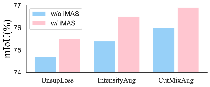
Figure 2: Effectiveness of iMAS on the unsupervised loss, intensity-based and CutMix augmentations, respectively.

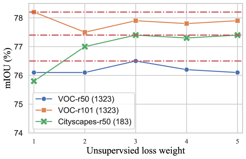
(a) $\lambda_{u}$

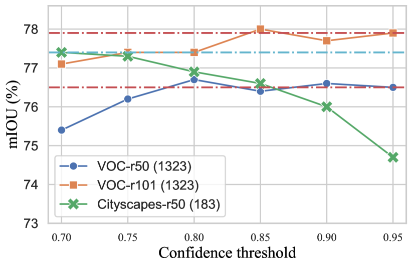
(b) $\tau$

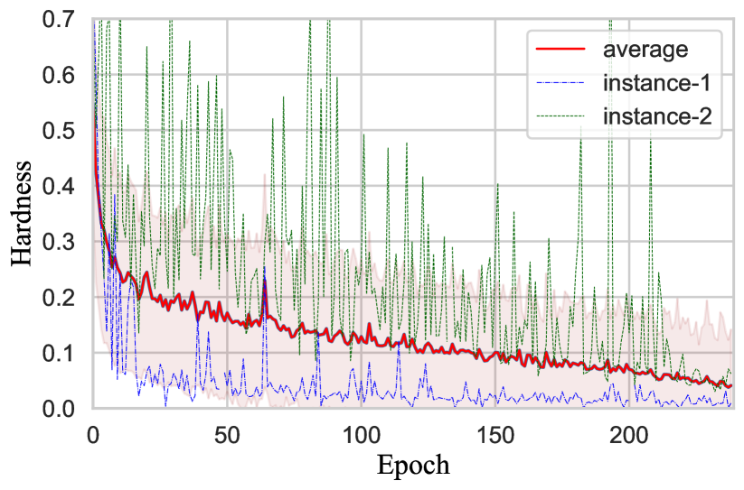
(c) hardness

Figure 3: We examine the effect of the loss weight and confidence threshold on VOC and Cityscapes under the 1/8 protocol in Figure (a) and (b), respectively. (c) shows how the mean instance hardness varies across the training course on Cityscapes under the 1/4 partition.

Cityscapes. In table 4, we evaluate our method on more challenging Cityscapes with ResNet-50 as the segmentation encoder. iMAS with output_stride$=8$ can achieve high mIOUs of 75.2%, 78.1%, 78.2%, 80.2%, in four different splits (1/16, 1/8, 1/4, 1/2), respectively. When output_stride$=16$, given only 186 labeled images, iMAS can obtain a notable performance gain of 10.3% against the supervised baseline and 6.5% against the previous best, U²PL. Not relying on any pseudo-rectifying networks [23] or extra self-supervised supervisions [41], iMAS achieves substantially better performance than the previous SOTAs, especially with fewer labels. Despite the simplicity of iMAS, the impressive performance further demonstrates the effectiveness and importance of our instance-specific and model-adaptive guidance. Surely, regardless of different semi-supervised approaches, we can see from Tables 4 that providing more labeled samples can easily improve the semi-supervised performance.

4.2 Ablations Studies

We conduct ablation studies in the 1/8 partitions of blended VOC and Cityscapes, and examine the impact of the model-adaptive guidance and approach-related hyper-parameters.

Effectiveness of model-adaptive guidance. The key of iMAS lies in the instance-specific and model-adaptive guidance. In Tab. 5, we conduct a series of experiments on VOC2012 dataset to demonstrate its effectiveness on three components, the unsupervised loss, intensity-based and CutMix augmentations, respectively. It can been seen from Fig. 2 that performing model-adaptive guidance can consistently improve the standard operations, yielding around 1% improvements on all standard counterparts. The powerfulness of strong augmentations can also be witnessed, as discussed in [45]. As a whole, iMAS can bring an improvement of 5.8% against the supervised baseline.

Impact of hyper-parameters. In Fig. 3, we investigate the influence of different $\lambda_{u}$ and $\tau$ on both datasets. It can be seen from Fig. 3(a) that iMAS is not very sensitive to the loss weight on VOC while a large $\lambda_{u}$ is beneficial for Cityscapes. By default, we set $\lambda_{u}=3$ for all runs. According to Fig. 3(b), we set $\tau=0.95$ for VOC and $\tau=0.7$ for Cityscapes as default settings. This is simply because Cityscapes is a more challenging dataset requiring better discriminating ability and using a high-threshold will prevent models effectively learning from unlabeled samples. We can see from Fig. 3(c) that both the mean and standard deviation of hardness evaluations on unlabeled data decrease as training processes and the model performance improves. Specifically, easy instances (e.g., Instance-1) can hold a low hardness from the very beginning, while the hardness of hard instances (e.g., Instance-2) fluctuates along the training process but eventually decreases.

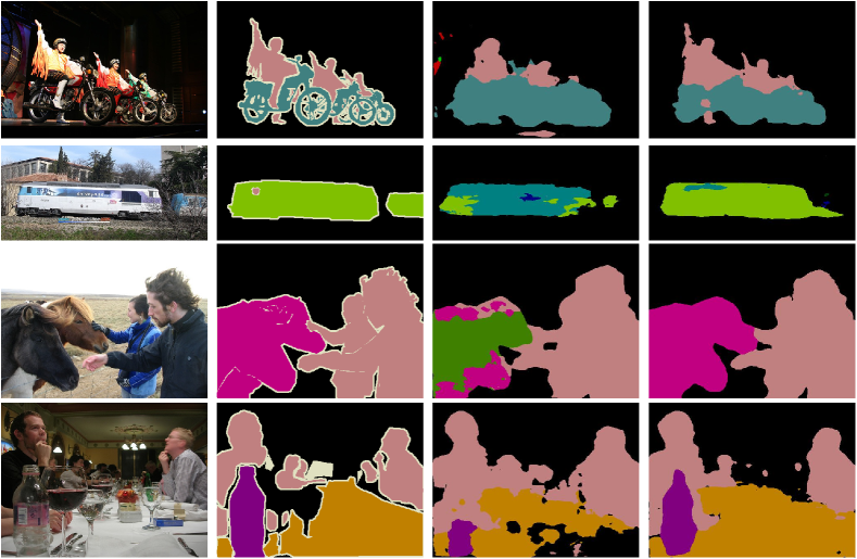
Figure 4: Qualitative results on Pascal VOC2012 using 183 fine labels. Columns from left to right denote the original images, the ground-truth, the supervised segmentation results, and the iMAS segmentation results, respectively.

Qualitative Results. We also present some segmentation results on Pascal VOC 2012 in Figure 4 under the 183 partition protocol, using the Resnet-101 as the encoder. We can see that many mis-classified pixels and ignored segmentation details like arms in the supervised-only results are corrected in iMAS.

5 Conclusion

In this paper, we highlight the instance uniqueness and propose iMAS, an instance-specific and model-adaptive supervision for semi-supervised semantic segmentation. Relying on our class-weighted symmetric hardness-evaluating strategies, iMAS treats each unlabeled instance discriminatively and employ model-adaptive augmentation and loss weighting strategies on each instance. Without introducing additional networks or losses, iMAS can remarkably improve the SSS performance. Our method is currently limited at requiring forward unlabeled samples twice to obtain hardness evaluations. We hope iMAS can inspire SSS studies to explore more model-related and simple approaches.

References

- [1] Inigo Alonso, Alberto Sabater, David Ferstl, Luis Montesano, and Ana C Murillo. Semi-supervised semantic segmentation with pixel-level contrastive learning from a class-wise memory bank. In ICCV, 2021.
- [2] Yoshua Bengio, Jérôme Louradour, Ronan Collobert, and Jason Weston. Curriculum learning. In ICML, 2009.
- [3] David Berthelot, Nicholas Carlini, Ekin D Cubuk, Alex Kurakin, Kihyuk Sohn, Han Zhang, and Colin Raffel. Remixmatch: Semi-supervised learning with distribution alignment and augmentation anchoring. In 8th International Conference on Learning Representations (ICLR), 2020.
- [4] David Berthelot, Nicholas Carlini, Ian Goodfellow, Nicolas Papernot, Avital Oliver, and Colin Raffel. Mixmatch: A holistic approach to semi-supervised learning. In NeurIPS, 2019.
- [5] Haw-Shiuan Chang, Erik Learned-Miller, and Andrew McCallum. Active bias: Training more accurate neural networks by emphasizing high variance samples. Advances in Neural Information Processing Systems, 30, 2017.
- [6] Liang-Chieh Chen, Yukun Zhu, George Papandreou, Florian Schroff, and Hartwig Adam. Encoder-decoder with atrous separable convolution for semantic image segmentation. In ECCV, 2018.
- [7] Xiaokang Chen, Yuhui Yuan, Gang Zeng, and Jingdong Wang. Semi-supervised semantic segmentation with cross pseudo supervision. In CVPR, 2021.
- [8] Marius Cordts, Mohamed Omran, Sebastian Ramos, Timo Rehfeld, Markus Enzweiler, Rodrigo Benenson, Uwe Franke, Stefan Roth, and Bernt Schiele. The cityscapes dataset for semantic urban scene understanding. In CVPR, 2016.
- [9] Ekin D Cubuk, Barret Zoph, Jonathon Shlens, and Quoc V Le. Randaugment: Practical automated data augmentation with a reduced search space. In Proceedings of the IEEE/CVF conference on computer vision and pattern recognition workshops, pages 702–703, 2020.
- [10] Jia Deng, Wei Dong, Richard Socher, Li-Jia Li, Kai Li, and Li Fei-Fei. Imagenet: A large-scale hierarchical image database. In CVPR, 2009.
- [11] Mark Everingham, SM Ali Eslami, Luc Van Gool, Christopher KI Williams, John Winn, and Andrew Zisserman. The pascal visual object classes challenge: A retrospective. IJCV, 2015.
- [12] Geoff French, Timo Aila, Samuli Laine, Michal Mackiewicz, and Graham Finlayson. Semi-supervised semantic segmentation needs strong, high-dimensional perturbations. In BMVC, 2020.
- [13] Ian J Goodfellow, Jonathon Shlens, and Christian Szegedy. Explaining and harnessing adversarial examples. In ICLR, 2015.
- [14] Jean-Bastien Grill, Florian Strub, Florent Altché, Corentin Tallec, Pierre Richemond, Elena Buchatskaya, Carl Doersch, Bernardo Avila Pires, Zhaohan Guo, Mohammad Gheshlaghi Azar, et al. Bootstrap your own latent-a new approach to self-supervised learning. Advances in neural information processing systems, 33:21271–21284, 2020.
- [15] Bharath Hariharan, Pablo Arbeláez, Lubomir Bourdev, Subhransu Maji, and Jitendra Malik. Semantic contours from inverse detectors. In 2011 international conference on computer vision, pages 991–998. IEEE, 2011.
- [16] Kaiming He, Xiangyu Zhang, Shaoqing Ren, and Jian Sun. Deep residual learning for image recognition. In CVPR, 2016.
- [17] Ruifei He, Jihan Yang, and Xiaojuan Qi. Re-distributing biased pseudo labels for semi-supervised semantic segmentation: A baseline investigation. In ICCV, 2021.
- [18] Hanzhe Hu, Fangyun Wei, Han Hu, Qiwei Ye, Jinshi Cui, and Liwei Wang. Semi-supervised semantic segmentation via adaptive equalization learning. In NeurIPS, 2021.
- [19] Wei-Chih Hung, Yi-Hsuan Tsai, Yan-Ting Liou, Yen-Yu Lin, and Ming-Hsuan Yang. Adversarial learning for semi-supervised semantic segmentation. In BMVC, 2018.
- [20] Mostafa S Ibrahim, Arash Vahdat, Mani Ranjbar, and William G Macready. Semi-supervised semantic image segmentation with self-correcting networks. In CVPR, 2020.
- [21] SouYoung Jin, Aruni RoyChowdhury, Huaizu Jiang, Ashish Singh, Aditya Prasad, Deep Chakraborty, and Erik Learned-Miller. Unsupervised hard example mining from videos for improved object detection. In Proceedings of the European Conference on Computer Vision (ECCV), pages 307–324, 2018.
- [22] Zhanghan Ke, Kaican Li Di Qiu, Qiong Yan, and Rynson WH Lau. Guided collaborative training for pixel-wise semi-supervised learning. In ECCV, 2020.
- [23] Donghyeon Kwon and Suha Kwak. Semi-supervised semantic segmentation with error localization network. In CVPR, 2022.
- [24] Xin Lai, Zhuotao Tian, Li Jiang, Shu Liu, Hengshuang Zhao, Liwei Wang, and Jiaya Jia. Semi-supervised semantic segmentation with directional context-aware consistency. In CVPR, 2021.
- [25] Dong-Hyun Lee et al. Pseudo-label: The simple and efficient semi-supervised learning method for deep neural networks. In ICML Workshop, 2013.
- [26] Yuyuan Liu, Yu Tian, Yuanhong Chen, Fengbei Liu, Vasileios Belagiannis, and Gustavo Carneiro. Perturbed and strict mean teachers for semi-supervised semantic segmentation. In CVPR, 2022.
- [27] Jonathan Long, Evan Shelhamer, and Trevor Darrell. Fully convolutional networks for semantic segmentation. In CVPR, 2015.
- [28] Robert Mendel, Luis Antonio de Souza, David Rauber, João Paulo Papa, and Christoph Palm. Semi-supervised segmentation based on error-correcting supervision. In ECCV, 2020.
- [29] Sudhanshu Mittal, Maxim Tatarchenko, and Thomas Brox. Semi-supervised semantic segmentation with high-and low-level consistency. TPAMI, 2019.
- [30] Takeru Miyato, Shin-ichi Maeda, Masanori Koyama, and Shin Ishii. Virtual adversarial training: a regularization method for supervised and semi-supervised learning. IEEE transactions on pattern analysis and machine intelligence, 41(8):1979–1993, 2018.
- [31] Samuel G Müller and Frank Hutter. Trivialaugment: Tuning-free yet state-of-the-art data augmentation. In Proceedings of the IEEE/CVF International Conference on Computer Vision, pages 774–782, 2021.
- [32] Yassine Ouali, Céline Hudelot, and Myriam Tami. An overview of deep semi-supervised learning. arXiv preprint arXiv:2006.05278, 2020.
- [33] Yassine Ouali, Céline Hudelot, and Myriam Tami. Semi-supervised semantic segmentation with cross-consistency training. In CVPR, 2020.
- [34] RB Prudêncio, José Hernández-Orallo, and Adolfo Martınez-Usó. Analysis of instance hardness in machine learning using item response theory. In Second International Workshop on Learning over Multiple Contexts in ECML, 2015.
- [35] Michael R Smith and Tony Martinez. A comparative evaluation of curriculum learning with filtering and boosting in supervised classification problems. Computational Intelligence, 32(2):167–195, 2016.
- [36] Michael R Smith, Tony Martinez, and Christophe Giraud-Carrier. An instance level analysis of data complexity. Machine learning, 95(2):225–256, 2014.
- [37] Kihyuk Sohn, David Berthelot, Chun-Liang Li, Zizhao Zhang, Nicholas Carlini, Ekin D Cubuk, Alex Kurakin, Han Zhang, and Colin Raffel. Fixmatch: Simplifying semi-supervised learning with consistency and confidence. In NeurIPS, 2020.
- [38] Kai Sheng Tai, Peter Bailis, and Gregory Valiant. Sinkhorn label allocation: Semi-supervised classification via annealed self-training. In ICML, 2021.
- [39] Antti Tarvainen and Harri Valpola. Mean teachers are better role models: Weight-averaged consistency targets improve semi-supervised deep learning results. In NeurIPS, 2017.
- [40] Yuandong Tian, Xinlei Chen, and Surya Ganguli. Understanding self-supervised learning dynamics without contrastive pairs. In International Conference on Machine Learning, pages 10268–10278. PMLR, 2021.
- [41] Yuchao Wang, Haochen Wang, Yujun Shen, Jingjing Fei, Wei Li, Guoqiang Jin, Liwei Wu, Rui Zhao, and Xinyi Le. Semi-supervised semantic segmentation using unreliable pseudo-labels. In CVPR, 2022.
- [42] Yikai Wang, Chengming Xu, Chen Liu, Li Zhang, and Yanwei Fu. Instance credibility inference for few-shot learning. In Proceedings of the IEEE/CVF conference on computer vision and pattern recognition, pages 12836–12845, 2020.
- [43] Qizhe Xie, Zihang Dai, Eduard Hovy, Minh-Thang Luong, and Quoc V Le. Unsupervised data augmentation for consistency training. In NeurIPS, 2020.
- [44] Fan Yang, Kai Wu, Shuyi Zhang, Guannan Jiang, Yong Liu, Feng Zheng, Wei Zhang, Chengjie Wang, and Long Zeng. Class-aware contrastive semi-supervised learning. In CVPR, 2022.
- [45] Lihe Yang, Wei Zhuo, Lei Qi, Yinghuan Shi, and Yang Gao. St++: Make self-training work better for semi-supervised semantic segmentation. In CVPR, 2022.
- [46] Jianlong Yuan, Yifan Liu, Chunhua Shen, Zhibin Wang, and Hao Li. A simple baseline for semi-supervised semantic segmentation with strong data augmentation. In ICCV, 2021.
- [47] Yuhui Yuan, Kuiyuan Yang, and Chao Zhang. Hard-aware deeply cascaded embedding. In ICCV, pages 814–823, 2017.
- [48] Sangdoo Yun, Dongyoon Han, Seong Joon Oh, Sanghyuk Chun, Junsuk Choe, and Youngjoon Yoo. Cutmix: Regularization strategy to train strong classifiers with localizable features. In ICCV, 2019.
- [49] Hongyi Zhang, Moustapha Cisse, Yann N Dauphin, and David Lopez-Paz. mixup: Beyond empirical risk minimization. arXiv preprint arXiv:1710.09412, 2017.
- [50] Zhen Zhao, Luping Zhou, Yue Duan, Lei Wang, Lei Qi, and Yinghuan Shi. Dc-ssl: Addressing mismatched class distribution in semi-supervised learning. In CVPR, 2022.
- [51] Zhen Zhao, Luping Zhou, Lei Wang, Yinghuan Shi, and Yang Gao. Lassl: Label-guided self-training for semi-supervised learning. In AAAI, 2022.
- [52] Yuanyi Zhong, Bodi Yuan, Hong Wu, Zhiqiang Yuan, Jian Peng, and Yu-Xiong Wang. Pixel contrastive-consistent semi-supervised semantic segmentation. In ICCV, 2021.
- [53] Tianyi Zhou, Shengjie Wang, and Jeffrey Bilmes. Curriculum learning by dynamic instance hardness. Advances in Neural Information Processing Systems, 33:8602–8613, 2020.
- [54] Yanning Zhou, Hang Xu, Wei Zhang, Bin Gao, and Pheng-Ann Heng. C3-semiseg: Contrastive semi-supervised segmentation via cross-set learning and dynamic class-balancing. In ICCV, 2021.
- [55] Yuliang Zou, Zizhao Zhang, Han Zhang, Chun-Liang Li, Xiao Bian, Jia-Bin Huang, and Tomas Pfister. Pseudoseg: Designing pseudo labels for semantic segmentation. In ICLR, 2021.