Exploring Physical Latent Spaces for High-Resolution Flow Restoration

Abstract

We explore training deep neural network models in conjunction with physics simulations via partial differential equations (PDEs), using the simulated degrees of freedom as latent space for a neural network. In contrast to previous work, this paper treats the degrees of freedom of the simulated space purely as tools to be used by the neural network. We demonstrate this concept for learning reduced representations, as it is extremely challenging to faithfully preserve correct solutions over long time-spans with traditional reduced representations, particularly for solutions with large amounts of small scale features. This work focuses on the use of such physical, reduced latent space for the restoration of fine simulations, by training models that can modify the content of the reduced physical states as much as needed to best satisfy the learning objective. This autonomy allows the neural networks to discover alternate dynamics that significantly improve the performance in the given tasks. We demonstrate this concept for various fluid flows ranging from different turbulence scenarios to rising smoke plumes. <ccs2012> <concept> <concept_id>10010147.10010371.10010352.10010379</concept_id> <concept_desc>Computing methodologies Physical simulation</concept_desc> <concept_significance>500</concept_significance> </concept> <concept> <concept_id>10010147.10010257.10010293.10010319</concept_id> <concept_desc>Computing methodologies Learning latent representations</concept_desc> <concept_significance>500</concept_significance> </concept> </ccs2012>

[500]Computing methodologies Physical simulation [500]Computing methodologies Learning latent representations

1 Introduction

Realistic simulation of natural phenomena is one of the ultimate goals of Computer Graphics research. Modeling and recreating such phenomena typically involves partial differential equations (PDEs) and thus numerical methods that aim for efficient computation of their solution. Despite the recent advances in numerical methods and computing power, many PDE problems of real-world scenarios, such as fluid simulation, require extremely costly calculations to resolve fine details, which are yet essential in the graphics context. Thus, using traditional numerical methods, which often require super-linear scaling in computation, remains challenging in practice. To minimize the costs of the computation, one can consider resolving the PDE in a reduced space, yet sacrificing the desired fine degrees of freedom both temporally and spatially. As an attractive compromise between computation and resolution, data-driven methods are becoming popular in many simulation problems [MJKW18, WKA*20, KSA*21].

In this paper, we present a data-driven simulation technique for PDE problems with a novel training method that explores using physical states as latent space for deep learning. In contrast to many previous studies [MJKW18, KAT*19, MDCL19, SFK*22], our latent space is not composed of the output or intermediate states of a neural network, but is rather made of the physical states of a PDE solver, such as velocity fields. We train a deep neural network (DNN) to exploit the content of a reduced PDE solver and shape it in a way that best satisfies the given learning objective, i.e., achieving solutions that are as accurate as possible at our target high resolution space. This shaping of the physical latent space gives the neural network a chance to discover modified dynamics and allows our model to better restore accurate high resolution solutions from them. Examples of the reduced and restored solutions are shown in Fig. Exploring Physical Latent Spaces for High-Resolution Flow Restoration.

Our training method consists of an encoder model transforming a coarse physical state using the degrees of freedom of a learnable latent space, a physics solver corresponding to a given PDE followed by an adjustment DNN, both operating in the reduced space, and a decoder turning the reduced state into the target high resolution space. To train our models with a physics solver, we adopt a differentiable simulator approach [HAL*20, HKT20, THM*21]. We let the encoder model learn the latent space representation without any other constraint than the restoration of the target solution. Therefore, an end-to-end training of this pipeline gives the encoder the complete autonomy to shape the reduced representation.

This paper demonstrates that the autonomy of our training method leads to a better performance than previous work, especially in terms of generalization. We apply our method to various complex, non-linear PDE problems, based on the Navier-Stokes equations, which are essential in the context of modeling fluid flows. For all the scenarios, our model produces more accurate high-resolution results in a longer temporal horizon than conventional and more tightly constrained models.

2 Related Work

Learning a PDE

The study of machine learning (ML) techniques for PDEs is getting more and more popular [CM87, KGH*03, BPK16]. A conventional direction when using ML for PDEs is to aim for the replacement of entire PDE solvers by neural network models that can efficiently approximate the solutions as accurately as possible [LKB18, KAT*19, WKM*20, BHKS21]. In this context, Fourier Neural Operator [LKA*21] and Neural Message Passing [BWW22] models have been introduced for learning PDEs, aiming at a better representation of full solvers with neural network models.

Instead of the pure ML-driven approach to solve target PDEs, an alternative approach exists in the form of hybrid methods that combine ML with traditional numerical methods. Among many different PDEs, fluid problems have received great attention due to their complex nature. For example, a learned model can replace the most expensive part of an iterative PDE solver for fluids [TSSP17, XYY18] or supplement inexpensive yet under-resolved simulations [UHT18, SMF20]. A regression forests model was also proposed for fast Lagrangian liquid simulations [LJS*15]. For smoke simulations in particular, efficient DNNs approaches synthesize high-resolution results from low-resolution versions [CT17, XFCT18, BLDL20] and convert low frame rate results into high frame rate versions [OL21].

Differentiable solvers

Recently, differentiable components for ML have been studied extensively, particularly when training neural network models in recurrent setups for spatio-temporal problems [AK17, dASA*18, TAST18, CRBD18, SF18, LLK19, WAG20, UBF*20, KSA*21, ZKB*21]. Consequently, a variety of differentiable programming frameworks have been developed for different domains [SC19, HAL*20, IEF*19, HKT20]. These differentiable frameworks allow neural networks to closely interact with PDE solvers, which provides the model with important feedback about the temporal evolution of the target problem from the recurrent evaluations. Targeting similar problems for temporal evolution, we employ a differentiable framework in our training procedure.

Latent space representations

Effectively utilizing latent spaces lies at the heart of many ML-based approaches for solving PDEs. A central role of the latent space is to embed important (often non-linear) information for the given training task into a set of reduced degrees of freedom. For example, with an autoencoder network architecture, the latent space can be used for discovering interpretable, low-dimensional dynamical models and their associated coordinates from high-dimensional data [CLKB19]. Moreover, thanks to their effectiveness in terms of embedding information and reducing the degrees of freedom, latent space solvers have been proposed for different problems such as advection-dominated systems [MLB21] and fluid flows [WKA*20, FMZF21]. While those studies typically focus on training equation-free evolution models, we focus on latent states that result from the interaction with a PDE solver. Neural network models have also been studied for the integration of a dynamical system with an ordinary differential equation (ODE) solver in the latent space [CRBD18]. This approach targets general neural network approximations with a simple physical model in the form of an ODE, whereas we focus on learning tasks for complex non-linear PDE systems.

Reduced solutions

The ability to learn underlying PDEs has allowed neural networks to improve reduced, approximate solutions. Residual correction models are trained to address numerical errors of PDE solvers [UBF*20]. Details at sub-grid scales are improved via learning discretizations of PDEs [BHHB19] and learning solvers [KSA*21, SFK*22] from high-resolution solutions. Moreover, multi-scale models with downsampled skip-connections have been used for super-resolution tasks of turbulent flows [FFT19]. These methods, however, typically employ a constrained solution manifold for the reduced representation. Indeed, the reduced solutions are produced using coarse-grained simulations with standard numerical methods, while our work shows the advantages of autonomously exploring the latent space representation through our joint training methodology.

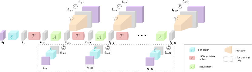
Figure 1: Architecture of our autonomous training approach for $N$ integrated solver steps. The initial state is encoded into the latent space, the solver and adjustment models are applied $N$ times, and the adjusted states are decoded into the fine space.

3 Exploring Physical Latent Spaces

For a given learning objective, our training method explores how neural network models can leverage the physical states of a PDE as latent space. Let $\mathbf{f}\in\mathbb{R}^{d_{f}}$ and $\mathbf{r}\in\mathbb{R}^{d_{r}}$ denote two discretized solutions of a PDE, a fine and a coarse version respectively, with $d_{r}\!\ll\!d_{f}$. We focus on the numerical integration of this target PDE problem and indicate the temporal evolution of each state as a subscript. A reference solution trajectory integrated from a given initial state $\mathbf{f}_{t}$ at time $t$ for $n$ steps is represented by the finite set of states $\{\mathbf{f}_{t},\mathbf{f}_{t+1},\cdots,\mathbf{f}_{t+n}\}$. Each reference state is integrated over time with a fixed time-step size using a numerical solver $\mathcal{P}_{f}$, i.e., $\mathbf{f}_{t+1}=\mathcal{P}_{f}(\mathbf{f}_{t})$. Similarly, we integrate a reduced state $\mathbf{r}_{t}$ over time using a corresponding numerical solver $\mathcal{P}_{r}$ at the reduced space, which we will call reduced solver henceforth, i.e., $\mathbf{r}_{t+1}=\mathcal{P}_{r}(\mathbf{r}_{t})$. In this paper, we focus on cases where the solver $\mathcal{P}$ is the same for both reduced and fine discretizations.

Our model takes the linear down-sampling of $\mathbf{f}_{t}$, i.e., $\mathbf{s}_{t}=\emph{lerp}(\mathbf{f}_{t})$, as input, and transforms it with the help of an encoder function $\mathcal{E}(\mathbf{s}|\theta_{E}):\mathbb{R}^{d_{r}}\rightarrow\mathbb{R}^{d_{r}}$, thus $\mathcal{E}(\mathbf{s}_{t}|\theta_{E})=\mathbf{\hat{s}}_{t}$. Then, we can obtain the next reduced state $\mathbf{r}_{t+1}=\mathcal{P}(\mathbf{\hat{s}}_{t})$. Moreover, in order to keep the reduced solution consistent with the encoded representation over time, the output of the reduced solver is transformed by an adjustment function, $\mathcal{A}(\mathbf{r}_{t+1}|\theta_{A})=\mathbf{\hat{r}}_{t+1}$. Thus, each reduced state $\mathbf{\hat{r}}_{t+i}$ is obtained by $i$ recurrent evaluations of the reduced solver and the adjustment function. Finally, a decoder function $\mathcal{D}(\mathbf{r}|\theta_{D}):\mathbb{R}^{d_{r}}\rightarrow\mathbb{R}^{d_{f}}$ restores a fine solution trajectory $\{\mathbf{\hat{f}}_{t},\mathbf{\hat{f}}_{t+1},\cdots,\mathbf{\hat{f}}_{t+n}\}$ from the reduced trajectory $\{\mathbf{\hat{r}}_{t},\mathbf{\hat{r}}_{t+1},\cdots,\mathbf{\hat{r}}_{t+n}\}$, thus $\mathbf{\hat{f}}_{t+i}=\mathcal{D}(\mathbf{\hat{r}}_{t+i}|\theta_{D})$. We model the encoder, adjustment, and decoder functions as DNNs in which trainable weights are denoted by $\theta_{E}$, $\theta_{A}$, and $\theta_{D}$, respectively.

The joint learning objective of the three DNNs is to minimize the error between the approximate solutions and their corresponding reference solutions, i.e., $||\mathbf{\hat{f}}_{t+i}-\mathbf{f}_{t+i}||_{2}$. To guide the adjustment model, we additionally minimize $\|\mathbf{\hat{r}}_{t+i}-\mathcal{E}(\mathbf{s}_{t+i}|\theta_{E})\|_{2}$. Thus, the final loss of our model is as follows:

$$\mathcal{L}=\sum_{i=1}^{N}\lambda_{hires}\times||\mathbf{\hat{f}}_{t+i}-\mathbf{f}_{t+i}||_{2}+\lambda_{latent}\times||\mathbf{\hat{r}}_{t+i}-\mathcal{E}(\mathbf{s}_{t+i}|\theta_{E})||_{2}$$ (1)

where $N$ denotes the number of integrated time-steps for training. Hence, at each training iteration, the gradients through all $N$ steps are computed for back-propagation and, consequently, all the models get jointly updated.

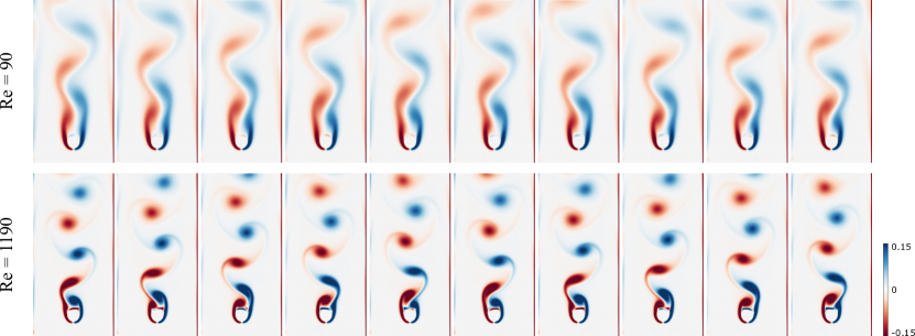
Figure 1: Two examples from the training data-set of the Karman vortex street scenario: Re = 90 and Re = 1190.

Fig. 1 shows the architecture of our approach. As the encoder does not receive any explicit constraint and has the complete freedom to autonomously explore the reduced space to arrive at a suitable representation, we denote this approach by ATO.

Comparisons and baselines

To illustrate the capabilities of our physical latent space, we compare ATO to two state-of-the-art models that operate in coarse space [SFK*22, UBF*20]. The former, denoted by Dil-ResNet in the following, represents a neural network model that aims at directly predicting solution states in the reduced space at each time-step. Hence, it does not make use of the reduced physics solver $\mathcal{P}$. On the other hand, the second variant [UBF*20], denoted by SOL, consists of a differentiable physics solver and a trainable corrector model that addresses numerical errors of the solution states. In both cases, unlike ATO, the models are trained to make reduced solutions by targeting the linear down-sampling of the reference.

We note that these state-of-the-art models output solutions that stay in the coarse space. As our ATO model aims at restoring high-resolution solutions using a decoder, a super-resolution model can transform these models’ reduced solutions into high-resolution ones. To this end, we feed the reduced states produced by the Dil-ResNet and SOL models to a super-resolution network specialized for spatio-temporal turbulence problems [FFT19], resulting in high-resolution states. Henceforth, these models will be denoted as Dil-ResNet + SR and SOL + SR.

4 Experiments

For each of the following scenarios, which are represented in 2D, the reference solution trajectories are generated for 200 steps from different initial conditions with a fixed time-step size. We focus on the velocity field for our restoration task and consider a four times coarser discretization for the reduced representation. More details about the experimental setups are given in the appendix.

4.1 Karman vortex street

We first consider a complex constrained PDE problem in the form of the Navier-Stokes equations. This problem is modeled as follows:

$$\partial{\mathbf{v}}/\partial{t}=-(\mathbf{v}\cdot\nabla)\mathbf{v}-\nabla{p}/\rho+\nu\nabla^{2}\mathbf{v}$$

$$\textrm{subject to}\quad\nabla\cdot\mathbf{v}=0$$

where $\mathbf{v}$ is the velocity, $p$ is the pressure, $\rho$ is the density and $\nu$ is the viscosity.

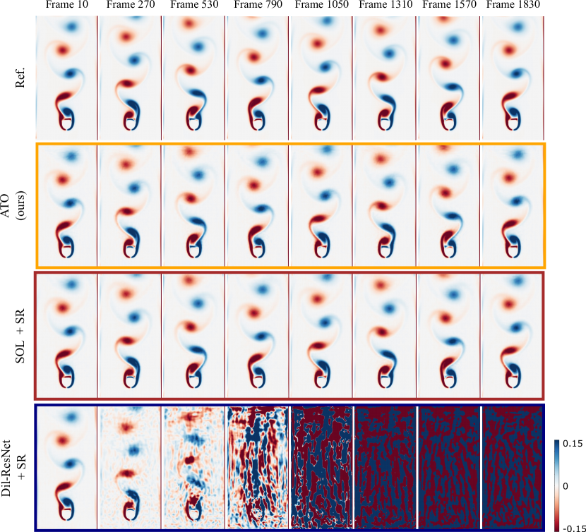
Figure 2: Restored frames of different models for the Karman vortex street scenario with Re = 850.

In this scenario, shown in Fig. 2 (left), a continuous inflow collides with a fixed circular obstacle. It creates an unsteady wake flow, which evolves differently depending on the Reynolds number. For the reference solutions, we use a numerical fluid solver that adopts the operator splitting scheme, Chorin projection for implicit pressure solve [Cho67], semi-Lagrangian advection [Sta99], and explicit integration for diffusion. We choose Reynolds numbers between $Re=90$ and $Re=1190$ for our training data-set, and Reynolds numbers from $Re=450$ to $Re=1400$ for testing. The encoder of our ATO setup takes the Reynolds number as an additional input in order to guide the exploration of the reduced space. The Dil-ResNet and SOL setups also receive the Reynolds number to let the models learn different physics evolutions. Finally, in order to be fair in our comparisons, the obstacle mask is applied to each state output by the Dil-ResNet solver. The domain of all target solutions is discretized with $128\times 256$ cells and has a staggered layout with closed boundaries, except for the bottom boundary for the constant inflow velocity and the top boundary that remains open. Although this setup targets a periodic evolution, the models are trained on more than one period in order to see a variety of initial states.

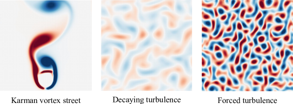
Figure 2: Example frames from the test data-set of each scenario.

4.2 Decaying and forced turbulence

This scenario is likewise based on the Navier-Stokes equations and is initialized with vortices randomly placed in the domain. We present two different sub-cases, one where the vortices are decaying over time without any external influence, and the other where an external force field $\mathbf{g}$ slows down the decaying motion of the vortex structures, enabling the creation of richer dynamics. The viscosity $\nu=0.1$ is used in both training data-sets, and the multiplicity of initial velocities and force fields enables a great variety of evolutions. Example frames of the decaying turbulence case are shown in Fig. 2 (middle). In the forced turbulence scenario, shown in Fig. 2 (right), as an additional degree of freedom for our learnable latent representation, we let the encoder of the ATO setup infer a latent force field $\mathbf{\hat{g}}$ that is integrated by the reduced solver. The linearly down-sampled field $\mathrm{lerp(\mathbf{g})}$ is used in the other setups. Each solution’s domain is discretized with $128^{2}$ cells and has a centered layout with periodic boundary conditions. A different randomized force sequence is generated for each simulation of the forced turbulence case, and the test sets are generated using different initial vortices and force fields than for training.

4.3 Smoke plume

This last scenario serves as a proof-of-concept of our method for more complex, practical graphics applications. Aiming for complex flow behavior driven by hot smoke plumes, we set up an initial smoke volume as a marker field with an arbitrary density distribution in a circular shape. The marker field is then passively advected by the velocity field and, at the same time, induces a buoyancy force via the Boussinesq approximation, that is influencing the velocity evolution. Therefore, the marker and velocity fields are tightly coupled. This scenario considers a more challenging problem of the Navier-Stokes equations than before, naturally making the fluid flow more interesting and providing a harder task for our model. The training and test data-sets are composed of smoke volumes initialized with random noise, with a fixed radius and position. The passive marker field is given as an input to our encoder and adjustment models, but its linearly down-sampled version is used in the reduced solver. Then, only the velocity field is up-sampled, and the high-resolution marker field is advected by the predicted velocity. The simulation domain is discretized with $128^{2}$ cells adopting a centered layout for the marker field, a staggered layout for the velocity field, and open boundary conditions.

4.4 Network architecture and training procedure

The encoder $\mathcal{E}(\cdot|\theta_{E})$ is implemented as a simple convolutional neural network (CNN) and the adjustment model is composed of convolutional layers that are interleaved with skip-connections. For the decoder, we adapt the multi-scale model for turbulent flows [FFT19], and the separate super-resolution network used in Dil-ResNet + SR and SOL + SR employs this same model. For all models, every convolutional layer except for the last one is followed by the Leaky ReLU activation function, except for Dil-ResNet which uses ReLU activations. We adopt circular padding for the periodic boundary condition problems and zero padding for the others. The architectures of the models are detailed in the appendix.

At each training iteration, for a given batch size, we randomly sample the initial states from the reference solution trajectories and integrate the approximate solution trajectories for $N$ steps. All our trainings use an Adam optimizer [KB14] and a decaying learning rate scheduling.

5 Results

We evaluate the trained models based on relative improvements over a baseline simulation. To make the baseline solutions, we apply the reduced solver without interactions with any neural network and up-sample the reduced states into the reference space with a linear interpolation. Errors are computed with respect to the reference solutions, hence an improvement of 100% would mean that the restored solutions are identical to the reference. We evaluate each model using the mean absolute error (MAE) and mean squared error (MSE) metrics, which we measure in both velocity and vorticity. We present the results of the models trained with the highest number of integrated steps for each scenario, as they show better performance in general.

5.1 Reduced representations

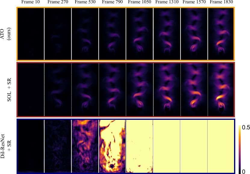
Figure 3: Absolute error in velocity for the different models, for the Karman vortex street scenario with Re = 850.

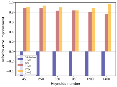
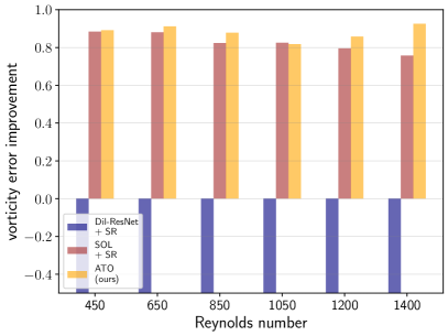
Figure 4: Velocity (left) and vorticity (right) error improvements for six different Reynolds numbers between 450 and 1400. The highest Reynolds number used for training is 1190. The ATO model generalizes better than the others.

The images of Fig. 3 show visual examples of the reduced representations for the Karman vortex street and forced turbulence scenarios, for different time-steps. The graphs of Fig. 4 show the quantified differences between the reduced states produced by the different trained models and the conventionally down-sampled reference states. We observe that our training procedure leads the latent representation to have vortex structures that are very similar to conventional down-sampling, while being considerably different quantitatively. Thus, we believe that the reduced representation of the ATO model stays physically meaningful for the numerical solver yet adds signals for accurately decoding high resolution states. We note that different training initializations of the same scenario produce latent representations that stay close to each other, which indicates that there exists a manifold of latent solutions that our ATO model converges to in order to get the best performance.

Figure 3: Reduced frames for the Karman vortex street case (left), and the forced turbulence case (right). The latent space of ATO (top) and the linearly down-sampled reference (bottom) are shown.

5.2 Karman vortex street

This example considers different vortex shedding behaviors depending on the Reynolds number of each simulation. We evaluate the models trained with 16 integrated steps on six test simulations with Reynolds numbers ranging from 450 to 1400, consisting of 2000 time-steps each. In this scenario, we test the extrapolation ability of the models both physically and temporally, with higher Reynolds number thus more turbulent simulations than for training, and ten times longer sequences.

Table 1 shows that ATO outperforms the other models, with a relative improvement of 91% (and 88%) in terms of velocity MAE (and vorticity), while SOL + SR improves the baseline by 84% (and 83%). On the other hand, the Dil-ResNet + SR model fails to retrieve the target simulation for more than 200 time-steps, and thus is incapable of generalization in this scenario. The temporal metrics shown in the appendix demonstrate the capability of ATO to correctly restore a solution for longer time ranges than the other models. More specifically, the distance between the reduced states and lerp(ref) show that the ATO model is the only one to have a consistent latent representation over time, which proves its better temporal extrapolation capabilities.

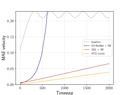
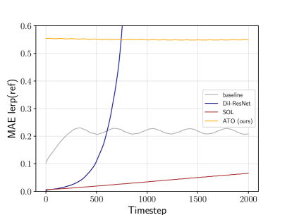
Figure 5: MAEs of recovered velocities (left) and distances of the reduced spaces to the down-sampled reference (right) over time for the Karman vortex street scenario.

Fig. 5 (left) shows examples of high-resolution frames produced by each model along with the spatial distribution of the absolute error in velocity, for Re = 1400. Although the visual quality of the different results seems equivalent at first sight, one can notice that the position of the vortices is more accurate in ATO’s outputs than SOL+SR’s. These results show that our ATO model, thanks to its latent space content, has learned to approximate the physical dynamics of the simulation more accurately.

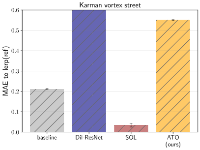
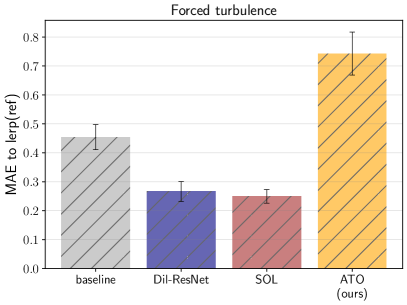
Figure 4: Distance between each model’s reduced space and the down-sampled reference. The error bars indicate the standard deviation over the test runs.

	Karman vortex street			Decaying turbulence			Forced turbulence
	($128\times 256$)			($128\times 128$)			($128\times 128$)
	MAE	MSE	runtime	MAE	MSE	runtime	MAE	MSE	runtime
Reference	N/A	N/A	28.2	N/A	N/A	14.1	N/A	N/A	17.9
Baseline	0.214	0.096	11.1	0.069	0.024	7.7	0.504	0.426	9.6
Dil-ResNet+SR	3580	1407	9.2	0.033	0.023	3.8	0.272	0.167	5.3
SOL+SR	0.035	0.005	20.0	0.013	0.005	12.8	0.256	0.137	14.2
ATO (ours)	0.020	0.002	20.4	0.012	0.005	11.5	0.133	0.040	12.4

Table 1: Summary of the MAE and MSE metrics, along with the runtime for one simulation of 100 frames (averaged over ten runs, in seconds).

5.3 Decaying turbulence

In this example, we consider initially chaotic turbulent flows that slowly decay over time. We evaluate the models trained with 16 integrated steps, on five random initializations, lasting 200 steps each.

Table. 1 shows that the ATO model yields greatly improved results with a relative improvement of 83% (and 80%) in terms of velocity MAE (and vorticity). However, in this more simple case, the SOL + SR model also improves the baseline significantly with 82% (and 78%) of relative improvement. Dil-ResNet + SR, however, only yields 53% (and 6%) of improvement. Examples frames for this scenario are shown in the appendix.

5.4 Forced turbulence

This complex fluid flow scenario considers the same experimental setup as in the previous case but with external forces, which leads to highly chaotic turbulent flows. We evaluate the models trained with 16 integrated steps, on five random initializations both in velocity and forcing, for 200 steps.

Table 1 shows that the ATO model significantly improves the baseline with a relative improvement of 74% (and 69%) in terms of velocity MAE (and vorticity). In comparison, SOL + SR improves by only 49% (and 43%) and Dil-ResNet + SR by 46% (and 38%). Therefore, in this complex case with external forcing and more turbulent flows, the ATO model particularly stands out. Fig. 5 (right) shows examples of high-resolution frames produced by each model along with the spatial distribution of the absolute error in velocity.

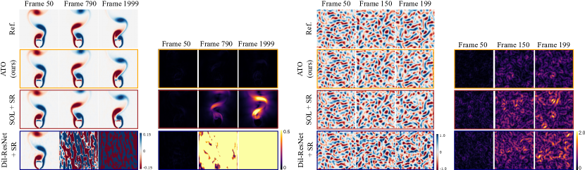
Figure 5: Example frames for all models along with the absolute error in velocity are shown for the Karman vortex street case with Re = 1400 (left) and for the forced turbulence case (right).

5.5 Smoke plume

In this last example, we consider complex flow behaviors created by hot smoke plumes that evolve from random circular densities. We evaluate our model trained with 32 integrated steps on five test simulations with different initial marker fields from which we perform a "warm-up" of 50 time-steps, in order to get interesting plume shapes.

Fig. 6 shows that, despite the increased difficulty of this challenging scenario, our ATO model succeeds at reconstructing a complex high-resolution plume of good quality. Indeed, our method presents an improvement of 35% on average over the baseline for 100 steps.

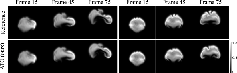
Figure 6: Example frames of the smoke plume scenario for two different initializations, for the ATO model.

5.6 Ablation study

In order to see the effects of each of its components, we evaluate our ATO model with differently ablated training setups for the forced turbulence scenario. Our ablation study includes the following models:

• No latent loss: we remove the second term of the loss in Eq. 1; consequently, our training does not constrain the adjusted states to match the encoder-induced latent space.

• No encoder: we omit the encoder such that the latent representation is constrained to be conventional linear down-sampling.

• No encoder & no latent loss: since the previous model’s reduced space is constrained to linear down-sampling, we test the same setup without the encoder and with no latent constraint.

• No solver: we replace the solver + adjustment part of our ATO model with the Dil-ResNet NN-solver in order to study the effect of a non-physical latent space.

• No adjustment: we evaluate a setup where the reduced simulation evolves without being adjusted.

• lerp(forces): we input a simple linear down-sampling of the force fields to the reduced solver, instead of their encoded representation.

	Velocity		Vorticity		Latent space
	MAE	MSE	MAE	MSE	MAE lerp(ref)
ATO (ours)	0.133	0.040	0.084	0.015	0.743
no latent loss	0.156	0.057	0.097	0.020	0.488
no encoder	0.259	0.146	0.156	0.48	0.253
no enc. & no lat. loss	0.284	0.174	0.167	0.055	0.322
no solver	0.737	1.073	0.578	0.651	0.713
no adjustment	0.409	0.339	0.212	0.085	0.568
lerp(forces)	0.944	1.725	0.429	0.325	0.682

Table 2: Results of the ablation study: we present the MAE and MSE in velocity and vorticity for each model, along with the distance between its reduced space and the down-sampled reference.

Table 2 shows that the encoder, physics solver, and adjustment components of our ATO model are essential for its good performance. Firstly, the no encoder and no encoder & no latent loss experiments confirm that, with lerp(ref) as initial reduced representation and without our encoder, the adjustment network was not able to find a latent representation that would lead to an optimal performance. Furthermore, the no latent loss ablation shows that the latent loss guiding the adjustment model via the encoder results in a better performance. Note that the performance of ATO significantly decreased when the encoder was absent, whereas the performance drop due to omitting the latent loss was relatively less significant. Secondly, the no solver and no adjustment experiments show that using a reduced physics solver in conjunction with an adjustment model is crucial for the good performance of our ATO model. Finally, the lerp(forces) experiment indicates that our encoder model failed to find a latent representation for the velocity that was compatible with an external factor conditioned to lerp.

All of the models tested in this ablation study gave comparable standard deviation values within the test set; thus, we did not include them in the table.

5.7 Runtime performance

For each scenario, we compare the runtime performance of the trained models with the reference’s, measuring timing for one simulation of 100 frames, averaged over ten different runs. For ATO, the computations start with the initial velocity inference by the encoder model and stop when all 100 frames are output by the decoder. All timings were computed using a single GeForce RTX 2080 Ti with 11GiB of VRAM.

Table 1 shows the summary of computational timings for the reference, baseline (reduced solver without any DNN model), and trained models. For all four cases, our ATO model yields improvement in runtime compared to the reference. For the Karman vortex street scenario, our ATO model speeds up the computations by 28%, against 29% for SOL+SR. Yet, as shown in Sec 5.2, ATO shows an improvement of the baseline MAE that is 7% better than SOL+SR. Similarly, for the forced turbulence case, the ATO model speeds up the computations by 18%, against 9% for SOL+SR, and improves the baseline MAE of 25% more than SOL+SR. For the smoke plume scenario, our ATO model speeds up the reference by 20% compared to 28% for the baseline, while improving the baseline MAE by 35%. We note that the Dil-ResNet + SR model often has the best runtime performance because it does not contain any numerical solver, but it has errors at least 50% higher than ATO and shows very poor temporal extrapolation capabilities.

Training our ATO model takes between one and three days depending on the physical scenario, on a Tesla V100 with 16GiB of VRAM.

6 Limitations and Future Work

These results show that our training method using the states of physics simulations as latent space of DNNs can facilitate the learning task for complex simulations. This provides a starting point for the exploration of physical latent spaces in many different problems. However, we note that our ATO model is not particularly standing out in a simple scenario like the decaying turbulence. Therefore, we can presume that the benefits of its unconventional reduced space are truly visible only when the PDE system is complex enough. In addition to the distance metric, more thorough analysis of latent space contents via, e.g., perceptual metrics, also remains our future work.

Moreover, our method has proven its capabilities in scenarios where force fields were inferred by our networks besides the velocity fields. In the forced turbulence case, the forces were external factors that were independent from the velocity data, thus our ATO model had no difficulty finding a latent representation that led to a superior performance. In Sec. 5.5, we showed that our model gave promising results in a scenario where the forces were internal, i.e. created by a marker field that was dependent of the latent velocity. That case opens interesting future work, such as finding the best reduced representations for the coupled marker and velocity fields.

Although we evaluated our model on various scenarios, its generalization for broader applications still remains a challenge. As our model allows for the efficient production of high-resolution simulations with a reduced solver, it is potentially attractive for editing physics simulations within the learned reduced space in real-time. Indeed, once a coarse initial frame is transformed into ATO’s latent space, it is easy to tweak the physical properties of the reduced solver (e.g., viscosity) or to add external factors, such that it can produce high-resolution simulations in a more interactive way. Accordingly, the adaptation of our ATO setup for three-dimensional problems is a promising topic for future work.

7 Conclusion

We have presented ATO, a model that leverages interactions between neural networks and a differentiable physics solver to autonomously explore reduced representations for high-resolution fluid restoration purposes. Our results show that deep neural networks can learn to develop new dynamics for specific learning objectives by using the simulated degrees of freedom as latent space. Our approach opens the path to the exploration of physical latent spaces for other PDEs, as well as different learning tasks than the restoration of details of fluid simulations.

8 Acknowledgments

This project has been funded by the Futur & Ruptures PhD program of the Fondation Mines-Telecom.

Appendix

1 Implementation details

We provide the implementation details with the code and data in the supplemental material, along with the neural network architectures. We refer to the guideline (i.e., README.md) to reproduce the results presented in this work. The code and trained models of our experiments will be published upon acceptance.

2 Experiments

In order to acquire a training data-set for each scenario, we generate a set of solution sequences of the given PDE problem. The PDEs from our experiments work with a continuous velocity field $\mathbf{v}$ in the two-dimensional space, i.e., $\mathbf{v}=[v_{x},v_{y}]^{T}$. Considering reference simulations on regularly discretized grids, we focus on exploring latent spaces (i.e., reduced representations) that are four times coarser than the reference.

2.1 Karman vortex street

This first example targets a complex PDE problem within a constrained setup, where the velocity field evolves over time while being constrained to be divergence free. We evaluate the incompressible Navier-Stokes equations for Newtonian fluids:

$$\frac{\partial{\mathbf{v}}}{\partial{t}}=-(\mathbf{v}\cdot\nabla)\mathbf{v}-\frac{\nabla{p}}{\rho}+\nu\nabla^{2}\mathbf{v}\quad\textrm{subject to}\quad\nabla\cdot\mathbf{v}=0$$ (1)

where $p$ is the pressure, $\rho$ is the density, and $\nu$ is the viscosity coefficient. The reference simulation domain is discretized with 128$\times$256 cells and a cell spacing of one using a staggered grid scheme. We use closed boundary conditions for the sides and open boundary conditions for the top of the domain; at the bottom, we set a constant inflow velocity. The continuous inflow collides with a fixed circular obstacle, which creates an unsteady wake flow that evolves differently depending on the Reynolds number. For the temporal discretization, the unit time step size is used. We generate 20 simulations of 200 steps each and randomly choose 5% of them for the validation set and the remaining 95% for the training set. We use Reynolds numbers in {90, 120, 140, 150, 160, 170, 180, 190, 200, 220, 290, 340, 390, 490, 540, 590, 690, 740, 790, 1190}, and we skip the first 2000 time-steps in order to let the flow stabilize. Both the least and most turbulent simulations of the training set are shown in Fig. 1.

In order to make our training more stable, we use pre-trained networks with eight integrated steps as warm starts for our final models. Each training uses 100 epochs with a batch size of ten. The learning rate starts from 4$\times$10^-4 and exponentially decays with a decaying rate of 0.9 every ten epochs. If divergence happens while training, we restart our training with a smaller learning rate. In this example, we compare all the models trained with 16 integrated steps. We also note that the encoder and adjustment models of ATO, the corrector of SOL, and the solver of Dil-ResNet take the Reynolds number as additional input.

The test set consists of six solution trajectories evaluated with Reynolds numbers in {450, 650, 850, 1050, 1200, 1400}. Example sequences of the test data and the inference results of different models are shown in Fig. 2, for $Re=850$, along with the spatial distribution of the velocity error in Fig. 3.

As can be seen on Fig. 4, which shows the velocity and vorticity error improvements of each model over the baseline, ATO presents the best generalization capabilities. Fig. 5 shows the temporal evolution of the velocity MAE and the distance between each model’s reduced space and lerp(ref).

2.2 Decaying turbulence

This example tackles the same incompressible Navier-Stokes equations, but with vortices intialized all over the physical space that slowly decay over time. In this scenario, the viscosity stays constant (equal to $0.1$) within the training and test data-sets. The reference simulation domain is discretized with 128² cells and a cell spacing of one. Both the discrete velocity and pressure values are stored at the center of each cell, and periodic boundary conditions are applied. For the temporal discretization, a time step size of 1.0 is used. The training data-set consists of 20 simulations of 200 steps each, which evolve from different initial velocity fields. We use randomly selected 5% for the validation set and the remaining 95% for the training set. An example sequence of the data is shown in Fig. 6. As in the Karman vortex street case, we first train our models with eight integrated steps as warm starts for the final models. We compare all the models trained with 16 integrated steps.

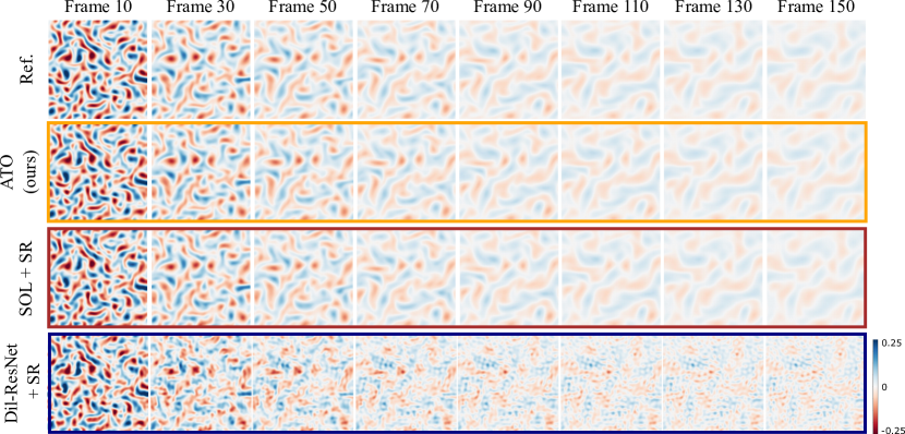
Figure 7: Example frames of a test case for different models for the decaying turbulence scenario.

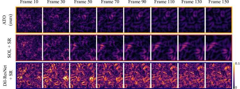
Figure 8: Absolute error in velocity for the different models, for the decaying turbulence scenario.

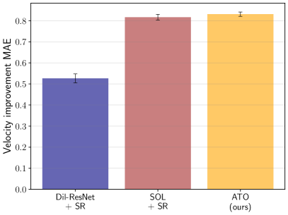
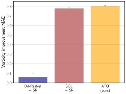
Figure 9: Velocity (left) and vorticity (right) error improvements for the decaying turbulence scenario. The ATO model improves the baseline the most for every test case.

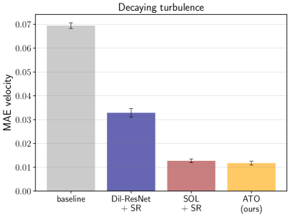
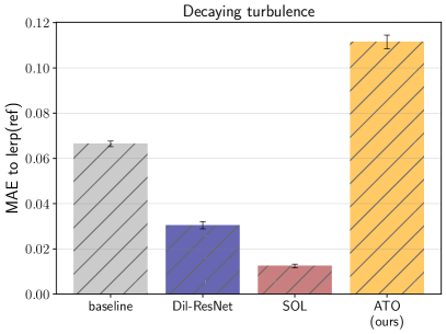
Figure 10: MAEs of recovered velocities (left) and distances of the reduced spaces to the down-sampled reference (right) for the decaying turbulence scenario.

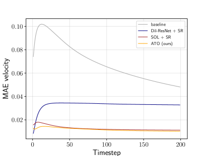
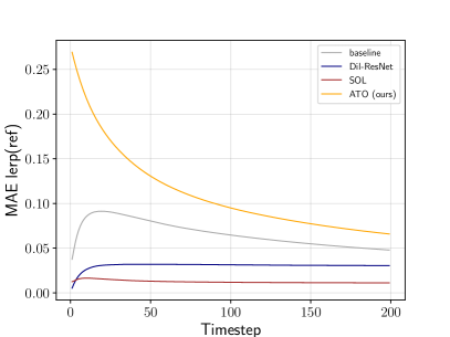
Figure 11: MAEs of recovered velocities (left) and distances of the reduced spaces to the down-sampled reference (right) over time for the decaying turbulence scenario.

The five test trajectories evolve from different initial velocity fields on a domain identical to the training one. Fig. 7 shows the inference results of the different models for one example, and Fig. 8 shows the spatial distribution of the error for the same example. Fig. 9 and Fig. 10 (left) show that our ATO model improves the baseline the most in both velocity and vorticity metrics, although SOL + SR shows a comparable performance. As shown in Fig. 11 and Fig. 10 (right), its latent space representation is more distant from the linearly down-sampled representation than the other models’, yet it shows a similar or better performance.

2.3 Forced turbulence

This case has the same experimental setup as the previous one, but with an external force sequence $\mathbf{g}(\mathbf{x},t)$ that is added to Eq. (1). This force sequence yields complex, chaotic evolutions of vortices over time. We use a different force sequence for each simulation trajectory, composed of 20 overlapping sine functions as follows:

$$g_{x}(\mathbf{x},t) =\sum_{i=1}^{20}a_{i}\sin(k_{i}\alpha_{i}\cdot\mathbf{x}+w_{i}t+\phi_{i})$$ (2)

$$g_{y}(\mathbf{x},t) =\sum_{i=1}^{20}a_{i}\sin(k_{i}\alpha_{i}\cdot\mathbf{x}+w_{i}t+\phi_{i})$$

where $a_{i}$ is the amplitude, $k_{i}$ is the wave number, $\alpha_{i}$ is the wave direction, $w_{i}$ is the frequency, and $\phi_{i}$ is the phase shift. These values are randomly sampled from uniform distributions as follows: $a_{i}\in[-0.1,0.1]$, $k_{i}\in\{6,8,10,12\}$, $w_{i}\in[-0.2,0.2]$, and $\phi_{i}\in[0,\pi]$. $\alpha_{i}$ is a random angle ($\in[0,2\pi]$). The composed sine functions are, then, evaluated over the domain mapped into $[0,2\pi]$ for each dimension.

For the temporal discretization, a time step size of 0.2 is used. The training data-set consists of 20 simulations of 200 steps each, which evolve from different initial velocity fields with different force sequences. We use randomly selected 5% for the validation set and the remaining 95% for the training set. An example sequence of the data is shown in Fig. 12. We use the models trained on the previous decaying turbulence case as warm starts for our final models, trained for 100 epochs. We compare all the models trained with 16 integrated steps. The encoder of ATO shares its weights for velocity and force in order to learn a unified operation for both reduced representations.

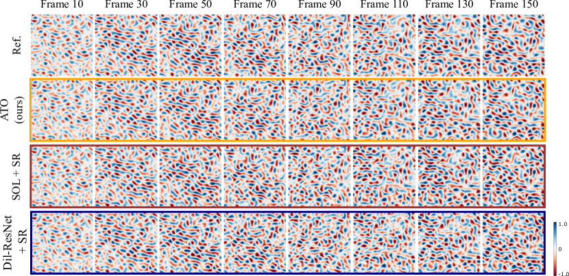
Figure 13: Example frames of a test case for different models for the forced turbulence scenario.

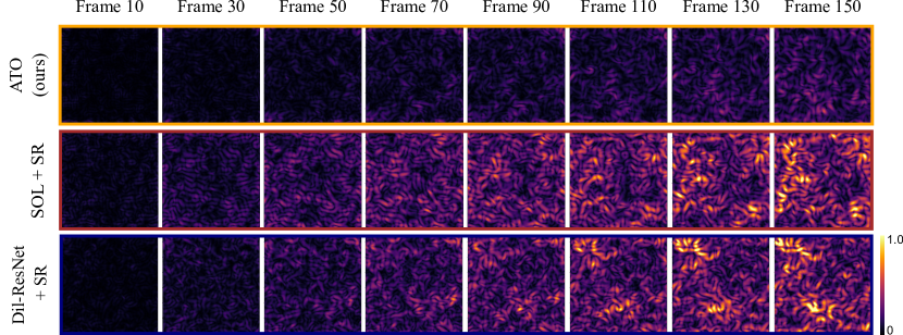
Figure 14: Absolute error in velocity for the different models, for the forced turbulence scenario.

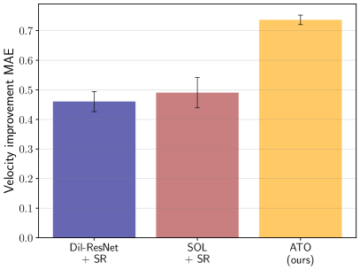
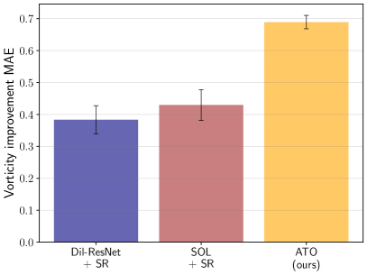
Figure 15: Velocity (left) and vorticity (right) error improvements for the forced turbulence scenario. The ATO model improves the baseline the most for every test case.

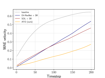
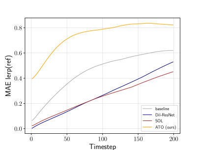
Figure 16: MAEs of recovered velocities (left) and distances of the reduced spaces to the down-sampled reference (right) over time for the forced turbulence scenario.

The five test trajectories evolve from both different initial velocity fields and different force field sequences. Fig. 13 shows the inference results of the different models for one example, and Fig. 14 shows the spatial distribution of the error for the same example. Fig. 15 shows that our ATO model improves the baseline the most in all five test cases in both velocity and vorticity metrics, while its latent space representation (Fig. 16) is more distant from the linearly down-sampled representation than the other models’.

2.4 Smoke plume

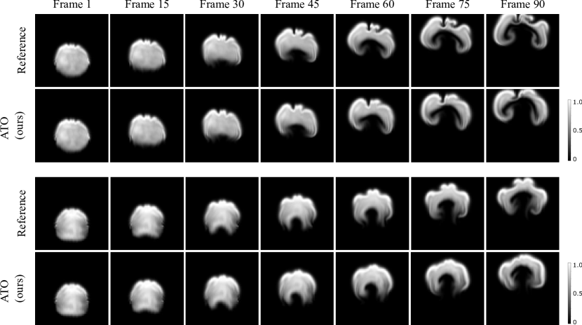
Figure 18: Example frames from our ATO model for two test cases of the smoke plume scenario.

This example represents a smoke volume of a circular shape, which is slowly rising up producing interesting swirling motions. A buoyancy force is produced by a passive marker field with a buoyancy factor of $0.25$ applied vertically. The training data-set consists of 20 simulations of 200 steps each with a time-step of $0.2$, which start from circular marker fields with a constant radius of $0.12$, but evolve differently due to the random initialization of the markers. We use randomly selected 5% for the validation set and the remaining 95% for the training set. An example sequence of the data is shown in Fig. 17. For this case, we use more integrated solver steps than the others. We first train our model with four, eight, and 16 integrated steps as warm starts for the final model. We apply our ATO model trained with 32 steps, for 100 epochs. Fig. 18 shows the inferences of our ATO model for different initializations.

3 Neural Network Architectures

In this section, we detail our network architectures for each model. We note that the practical implementations of all the models can be found in the supplemental code.

The encoder of the ATO setup consists of two convolutional layers with 32 and 16 features each with a kernel size of five. Each convolutional layer is followed by the Leaky ReLU activation function. A last layer with two features and the same kernel size but without the activation infers the final encoded output. This model has approximately 15k trainable weights.

The adjustment of the ATO setup and the corrector of SOL ([UBF*20]) employ an identical network model. This model consists of a first convolutional layer with 32 features and a kernel size of five, followed by five blocks of two convolutional layers with 32 features each and a kernel size of five. Each layer is followed by the Leaky ReLU activation function, and each block is connected to the next with a skip-connection. A last layer with two features follows with the same kernel size yet without the activation. This architecture has approximately 260k trainable weights.

The decoder used for the ATO setup and the super-resolution model from Dil-ResNet + SR and SOL + SR are adapted from the multi-scale architecture of [FFT19], such that the total number of trainable weights is close to 97k.

The Dil-ResNet model is adapted from the architecture of the state-of-the-art network model proposed for turbulent flow problems [SFK*22]. This model has a first convolutional layer with 32 features with a kernel size of three and no activation. It is followed by four identical blocks of seven convolutional layers with 32 features each with a kernel size of three and varying dilation rates from one to eight (respectively: 1, 2, 4, 8, 4, 2, 1). Each layer is followed by the ReLU activation function, and each block is linked to the next via a skip-connection. A last layer with two features follows with the same kernel size yet without the activation. This model has a similar number of trainable weights as the adjustment model’s (i.e., 260k). We note that a larger model did not improve the performance. Contrary to the other models, Dil-ResNet is trained for only one step at a time and uses a MSE loss.

For the Karman vortex street and smoke plume cases, we adopt zero-padding, and for the forced and decaying turbulence cases, which use periodic boundary conditions, we use periodic padding for all models.

4 Training hyper-parameters

In this section, we detail the choice of hyper-parameters for the different trained models.

Firstly, the code of the SOL model from [UBF*20] was released publicly, which enabled an easy reproduction of their experiments. Secondly, the learning setup of the Dil-ResNet model from [SFK*22] was precisely described in the article. We extensively tested the various hyper-parameters and chose the Dil-ResNet model over Con-Dil-ResNet (i.e., without the additional loss constraint) because it performed better in our physical scenarios. For training, we chose a Gaussian noise with $\sigma=0.01$ for all scenarios. Lastly, for our ATO setup, we chose the depth of the models by making a compromise between performance and runtime/resources. For the learning rate and batch size, since the physics solver made the models harder to train, we chose the values that best stabilized our training. Our loss being divided in two terms of different orders of magnitude (a high-resolution term and a low-resolution one), we set $\lambda_{hires}$ to $1$ for all scenarios and $\lambda_{latent}=1$ for the Karman vortex street case, $\lambda_{latent}=1$ = 10 for the decaying turbulence, $\lambda_{latent}=100$ for the forced turbulence and $\lambda_{latent}=10$ for the smoke plume.

Figure 6: Example frames from one simulation of the training data-set of the decaying turbulence scenario.

Figure 12: Example frames from one simulation of the training data-set of the forced turbulence scenario.

Figure 17: Example frames from one simulation of the training data-set of the smoke plume scenario.

References

- [AK17] Brandon Amos and J. Kolter “OptNet: Differentiable Optimization as a Layer in Neural Networks” In Proceedings of the 34th International Conference on Machine Learning - Volume 70, ICML’17 Sydney, NSW, Australia: JMLR.org, 2017, pp. 136–145
- [BHHB19] Yohai Bar-Sinai, Stephan Hoyer, Jason Hickey and Michael P Brenner “Learning data-driven discretizations for partial differential equations” In Proceedings of the National Academy of Sciences 116.31 National Acad Sciences, 2019, pp. 15344–15349
- [BHKS21] Kaushik Bhattacharya, Bamdad Hosseini, Nikola B. Kovachki and Andrew M. Stuart “Model Reduction and Neural Networks for Parametric PDEs” In The SMAI journal of computational mathematics 7, 2021, pp. 121–157 DOI: 10.5802/smai-jcm.74
- [BLDL20] Kai Bai, Wei Li, Mathieu Desbrun and Xiaopei Liu “Dynamic Upsampling of Smoke through Dictionary-Based Learning” In ACM Transactions on Graphics 40.1, 2020, pp. 4:1–4:19 DOI: 10.1145/3412360
- [BPK16] Steven L Brunton, Joshua L Proctor and J Nathan Kutz “Discovering governing equations from data by sparse identification of nonlinear dynamical systems” In Proceedings of the National Academy of Sciences 113.15 National Acad Sciences, 2016, pp. 3932–3937
- [BWW22] Johannes Brandstetter, Daniel E. Worrall and Max Welling “Message Passing Neural PDE Solvers” In International Conference on Learning Representations, 2022 URL: https://openreview.net/forum?id=vSix3HPYKSU
- [Cho67] Alexandre Joel Chorin “The numerical solution of the Navier-Stokes equations for an incompressible fluid” In Bulletin of the American Mathematical Society 73.6, 1967, pp. 928–931
- [CLKB19] Kathleen Champion, Bethany Lusch, J. Kutz and Steven L. Brunton “Data-Driven Discovery of Coordinates and Governing Equations” In Proceedings of the National Academy of Sciences 116.45 National Academy of Sciences, 2019, pp. 22445–22451 DOI: 10.1073/pnas.1906995116
- [CM87] James P Crutchfield and Bruce S McNamara “Equations of motion from a data series” In Complex systems 1.417-452, 1987, pp. 121
- [CRBD18] Tian Qi Chen, Yulia Rubanova, Jesse Bettencourt and David K Duvenaud “Neural ordinary differential equations” In Advances in neural information processing systems, 2018, pp. 6571–6583
- [CT17] Mengyu Chu and Nils Thuerey “Data-Driven Synthesis of Smoke Flows with CNN-Based Feature Descriptors” In ACM Trans. Graph. 36.4, 2017, pp. 69:1–69:14 DOI: 10.1145/3072959.3073643
- [dASA*18] Filipe Avila Belbute-Peres et al. “End-to-End Differentiable Physics for Learning and Control” In Advances in Neural Information Processing Systems 31 Curran Associates, Inc., 2018 URL: https://proceedings.neurips.cc/paper/2018/file/842424a1d0595b76ec4fa03c46e8d755-Paper.pdf
- [FFT19] Kai Fukami, Koji Fukagata and Kunihiko Taira “Super-resolution reconstruction of turbulent flows with machine learning” In Journal of Fluid Mechanics 870 Cambridge University Press, 2019, pp. 106–120
- [FMZF21] Kai Fukami, Takaaki Murata, Kai Zhang and Koji Fukagata “Sparse Identification of Nonlinear Dynamics with Low-Dimensionalized Flow Representations” In Journal of Fluid Mechanics 926 Cambridge University Press, 2021 DOI: 10.1017/jfm.2021.697
- [HAL*20] Yuanming Hu et al. “DiffTaichi: Differentiable Programming for Physical Simulation” In International Conference on Learning Representations (ICLR), 2020
- [HKT20] Philipp Holl, Vladlen Koltun and Nils Thuerey “Learning to Control PDEs with Differentiable Physics” In International Conference on Learning Representations (ICLR), 2020
- [IEF*19] Mike Innes et al. “A differentiable programming system to bridge machine learning and scientific computing” In arXiv 1907.07587, 2019
- [KAT*19] Byungsoo Kim et al. “Deep Fluids: A Generative Network for Parameterized Fluid Simulations” In Computer Graphics Forum The Eurographics AssociationJohn Wiley & Sons Ltd., 2019 DOI: 10.1111/cgf.13619
- [KB14] Diederik Kingma and Jimmy Ba “Adam: A Method for Stochastic Optimization” In arXiv:1412.6980 [cs], 2014 arXiv:1412.6980 [cs]
- [KGH*03] Ioannis G Kevrekidis et al. “Equation-free, coarse-grained multiscale computation: Enabling mocroscopic simulators to perform system-level analysis” In Communications in Mathematical Sciences 1.4 International Press of Boston, 2003, pp. 715–762
- [KSA*21] Dmitrii Kochkov et al. “Machine Learning–Accelerated Computational Fluid Dynamics” In Proceedings of the National Academy of Sciences 118.21 National Academy of Sciences, 2021 DOI: 10.1073/pnas.2101784118
- [LJS*15] Lubor Ladický et al. “Data-Driven Fluid Simulations Using Regression Forests” In ACM Trans. Graph. 34.6, 2015, pp. 199:1–199:9 DOI: 10.1145/2816795.2818129
- [LKA*21] Zongyi Li et al. “Fourier Neural Operator for Parametric Partial Differential Equations” In International Conference on Learning Representations, 2021 URL: https://openreview.net/forum?id=c8P9NQVtmnO
- [LKB18] Bethany Lusch, J. Kutz and Steven L. Brunton “Deep Learning for Universal Linear Embeddings of Nonlinear Dynamics” In Nature Communications 9.1 Nature Publishing Group, 2018, pp. 4950 DOI: 10.1038/s41467-018-07210-0
- [LLK19] Junbang Liang, Ming Lin and Vladlen Koltun “Differentiable Cloth Simulation for Inverse Problems” In Advances in Neural Information Processing Systems, 2019, pp. 771–780
- [MDCL19] Arvind Mohan, Don Daniel, Michael Chertkov and Daniel Livescu “Compressed Convolutional LSTM: An Efficient Deep Learning framework to Model High Fidelity 3D Turbulence” In arXiv:1903.00033, 2019
- [MJKW18] Jeremy Morton, Antony Jameson, Mykel J Kochenderfer and Freddie Witherden “Deep dynamical modeling and control of unsteady fluid flows” In Advances in Neural Information Processing Systems, 2018
- [MLB21] Romit Maulik, Bethany Lusch and Prasanna Balaprakash “Reduced-order modeling of advection-dominated systems with recurrent neural networks and convolutional autoencoders” In Physics of Fluids 33.3 American Institute of Physics, 2021, pp. 037106 DOI: 10.1063/5.0039986
- [OL21] Young Jin Oh and In-Kwon Lee “Two-step Temporal Interpolation Network Using Forward Advection for Efficient Smoke Simulation” In Computer Graphics Forum 40.2, 2021, pp. 355–365 DOI: 10.1111/cgf.142638
- [SC19] Samuel S Schoenholz and Ekin D Cubuk “JAX, MD: End-to-End Differentiable, Hardware Accelerated, Molecular Dynamics in Pure Python” In arXiv:1912.04232, 2019
- [SF18] Connor Schenck and Dieter Fox “SPNets: Differentiable Fluid Dynamics for Deep Neural Networks” In Conference on Robot Learning, 2018, pp. 317–335
- [SFK*22] Kim Stachenfeld et al. “Learned Simulators for Turbulence” In International Conference on Learning Representations, 2022 URL: https://openreview.net/forum?id=msRBojTz-Nh
- [SMF20] Justin Sirignano, Jonathan F. MacArt and Jonathan B. Freund “DPM: A Deep Learning PDE Augmentation Method with Application to Large-Eddy Simulation” In Journal of Computational Physics 423, 2020, pp. 109811 DOI: 10.1016/j.jcp.2020.109811
- [Sta99] Jos Stam “Stable Fluids” In SIGGRAPH ’99 ACM, 1999, pp. 121–128 DOI: 10.1145/311535.311548
- [TAST18] Marc Toussaint, Kelsey Allen, Kevin Smith and Joshua B Tenenbaum “Differentiable physics and stable modes for tool-use and manipulation planning” In Robotics: Science and Systems, 2018
- [THM*21] Nils Thuerey et al. “Physics-based Deep Learning” In arXiv:2109.05237 [physics], 2021 arXiv:2109.05237 [physics]
- [TSSP17] Jonathan Tompson, Kristofer Schlachter, Pablo Sprechmann and Ken Perlin “Accelerating Eulerian Fluid Simulation With Convolutional Networks” In Proceedings of Machine Learning Research, 2017, pp. 3424–3433
- [UBF*20] Kiwon Um et al. “Solver-in-the-loop: learning from differentiable physics to interact with iterative PDE-solvers” In Advances in Neural Information Processing Systems 33, 2020 arXiv:2007.00016
- [UHT18] Kiwon Um, Xiangyu Hu and Nils Thuerey “Liquid Splash Modeling with Neural Networks” In Computer Graphics Forum 37.8, 2018, pp. 171–182 DOI: 10.1111/cgf.13522
- [WAG20] Wujie Wang, Simon Axelrod and Rafael Gómez-Bombarelli “Differentiable Molecular Simulations for Control and Learning” In arXiv:2003.00868, 2020
- [WKA*20] S. Wiewel et al. “Latent Space Subdivision: Stable and Controllable Time Predictions for Fluid Flow” In Proceedings of the ACM SIGGRAPH/Eurographics Symposium on Computer Animation, SCA ’20 Goslar, DEU: Eurographics Association, 2020, pp. 1–11 DOI: 10.1111/cgf.14097
- [WKM*20] Rui Wang et al. “Towards Physics-Informed Deep Learning for Turbulent Flow Prediction” In Proceedings of the 26th ACM SIGKDD International Conference on Knowledge Discovery & Data Mining, KDD ’20 New York, NY, USA: Association for Computing Machinery, 2020, pp. 1457–1466 DOI: 10.1145/3394486.3403198
- [XFCT18] You Xie, Erik Franz, Mengyu Chu and Nils Thuerey “tempogan: A temporally coherent, volumetric gan for super-resolution fluid flow” In ACM Transactions on Graphics (TOG) 37.4 ACM, 2018, pp. 1–15
- [XYY18] Xiangyun Xiao, Cheng Yang and Xubo Yang “Adaptive Learning-Based Projection Method for Smoke Simulation” In Computer Animation and Virtual Worlds 29.3-4, 2018, pp. e1837 DOI: 10.1002/cav.1837
- [ZKB*21] Jiawei Zhuang et al. “Learned Discretizations for Passive Scalar Advection in a Two-Dimensional Turbulent Flow” In Physical Review Fluids 6.6 American Physical Society, 2021, pp. 064605 DOI: 10.1103/PhysRevFluids.6.064605