Anomalous magnetohydrodynamics with temperature-dependent electric conductivity and application to the global polarization

Abstract

We have derived the solutions of the relativistic anomalous magnetohydrodynamics with longitudinal Bjorken boost invariance and transverse electromagnetic fields in the presence of temperature or energy density dependent electric conductivity. We consider the equations of states in a high temperature limit or in a high chiral chemical potential limit. We obtain both perturbative analytic solutions up to the order of $\hbar$ and numerical solutions in our configurations of initial electromagnetic fields and Bjorken flow velocity. Our results show that the temperature or energy density dependent electric conductivity plays an important role to the decaying of the energy density and electromagnetic fields. We also implement our results to the splitting of global polarization for $\Lambda$ and $\overline{\Lambda}$ hyperons induced by the magnetic fields. Our results for the splitting of global polarization disagree with the experimental data in low energy collisions, which implies that the contribution from gradient of chemical potential may dominate in the low energy collisions.

I Introduction

Recently, strong electromagnetic (EM) fields (of order $10^{17}-10^{18}$Gauss (Skokov:2009qp, ; Bzdak:2011yy, ; Deng:2012pc, ; Roy:2015coa, )) generated in the relativistic heavy ion collisions provide a platform to study the novel quantum transport phenomena and non-linear quantum electrodynamics.

The strong magnetic fields can induce the chiral magnetic effect (CME) (Vilenkin:1980fu, ; Kharzeev:2007tn, ; kharzeev2008effects, ; Fukushima:2008xe, ) associated with the chiral anomaly, chiral separation effect (Aghababaie:2003iw, ) and chiral magnetic wave (Kharzeev:2010gd, ; Burnier:2011bf, ). While the electric fields can cause chiral electric separation effect (Huang:2013iia, ; Pu:2014cwa, ; Jiang:2014ura, ; Pu:2014fva, ) and other novel nonlinear EM responses in chiral systems (Pu:2014fva, ; Chen:2016xtg, ; Gorbar:2016qfh, ; Gorbar:2016sey, ; Gorbar:2016ygi, ; Gorbar:2017cwv, ). These chiral transport phenomena are naturally connected to the Schwinger mechanism (Fukushima:2010vw, ; Warringa:2012bq, ; Copinger:2018ftr, ; Copinger:2020nyx, ; Copinger:2022jgg, ). More discussions and references can be found in recent reviews (Kharzeev:2012ph, ; Kharzeev:2015znc, ; Liao:2014ava, ; Miransky:2015ava, ; Huang:2015oca, ; Fukushima:2018grm, ; Bzdak:2019pkr, ; Zhao:2019hta, ; Gao:2020vbh, ; Shovkovy:2021yyw, ). To understand and describe these chiral transport, the quantum kinetic theory or named Wigner function approaches, as an microscopic effective theory has been widely discussed (Gao:2012ix, ; Son:2012zy, ; Chen:2012ca, ; Stephanov:2012ki, ; Manuel:2013zaa, ; Chen:2013dca, ; Manuel:2014dza, ; Chen:2014cla, ; Chen:2015gta, ; Hidaka:2016yjf, ; Mueller:2017lzw, ; Hidaka:2017auj, ; Gao:2017gfq, ; Liu:2018xip, ; Hidaka:2018ekt, ; Huang:2018wdl, ; Hidaka:2018mel, ; Gao:2018wmr, ; Gao:2019znl, ; Wang:2019moi, ; Li:2019qkf, ; Weickgenannt:2019dks, ; Hattori:2019ahi, ; Lin:2019ytz, ; Lin:2019fqo, ; Gao:2019zhk, ; Weickgenannt:2020aaf, ; Weickgenannt:2020sit, ; Liu:2020flb, ; Huang:2020wrr, ; Yamamoto:2020zrs, ; Yang:2020hri, ; Wang:2021qnt, ; Sheng:2021kfc, ; Luo:2021uog, ; Weickgenannt:2021cuo, ; Hidaka:2022dmn, ; Fang:2022ttm, ) (also see Ref. (Hidaka:2022dmn, ; Gao:2020vbh, ; Gao:2020pfu, ) for the recent reviews on quantum kinetic theory).

It is still challenging to search the CME signal in the relativistic heavy ion collision at Relativistic Heavy Ion Collider (RHIC) (STAR:2009wot, ; STAR:2009tro, ; Wang:2012qs, ; STAR:2013ksd, ; STAR:2013zgu, ; STAR:2014uiw, ; Tribedy:2017hwn, ; STAR:2019xzd, ) and Large Hadron Collider (LHC) (ALICE:2012nhw, ; CMS:2016wfo, ; CMS:2017lrw, ). Although many possible correlators or observables have been proposed (STAR:2013ksd, ), the background contributions from, e.g., the transverse momentum conservation (Pratt:2010zn, ; Bzdak:2012ia, ; Ajitanand:2010rc, ; Magdy:2017yje, ; Tang:2019pbl, ), local charge conservation (Schlichting:2010qia, ) and non-flow correlations (Xu:2017zcn, ; Xu:2020sln, ), cannot be neglected. Nevertheless, the recent isobar collisions (Voloshin:2010ut, ) in STAR measurements (STAR:2021mii, ) do not observe the CME signature that satisfies the predefined criteria. It requires the future systematical studies on CME.

Another interesting phenomena related to the chiral transport and EM fields is the global and local polarization of $\Lambda$ and $\overline{\Lambda}$ hyperons (Liang:2004ph, ; Liang:2004xn, ; Gao:2007bc, ). The global polarization has been measured by the STAR experiments (STAR:2017ckg, ) and been widely studied in several models (Karpenko:2016jyx, ; Li:2017slc, ; Xie:2017upb, ; Sun:2017xhx, ; Shi:2017wpk, ; Wei:2018zfb, ; Wu:2019eyi, ; Wu:2020yiz, ; Fu:2020oxj, ; Ryu:2021lnx, ; Wu:2022mkr, ) (also see recent reviews (Wang:2017jpl, ; Becattini:2020ngo, ; Becattini:2020sww, ; Gao:2020vbh, )). Meanwhile, the local spin polarization, in Au+Au collisions at $\sqrt{s_{NN}}=$ 200 GeV has been measured (STAR:2019erd, ) and studied (Liu:2020dxg, ; Liu:2021uhn, ; Becattini:2021suc, ; Yi:2021ryh, ; Ryu:2021lnx, ; Yi:2021unq, ; Wu:2022mkr, ). Several studies have pointed out that the splitting of global polarization of $\Lambda$ and $\overline{\Lambda}$ hyperons may be induced by the EM fields (Muller:2018ibh, ; Guo:2019joy, ; Buzzegoli:2022qrr, ; Xu:2022hql, ) and gradient of baryon chemical potential (Ryu:2021lnx, ; Fu:2022myl, ; Wu:2022mkr, ). Therefore, the further studies on the EM fields and their evolution are also required in this field.

On the other hand, strong EM fields make the studying of the non-linear electrodynamics be possible. The light-by-light scattering (ATLAS:2017fur, ), matter generation directly from photons (STAR:2019wlg, ; Zha:2018tlq, ), the vacuum birefringence (Hattori:2012je, ; Hattori:2012ny, ; Hattori:2020htm, ; STAR:2019wlg, ; Hattori:2022uzp, ; Adler:1971wn, ) have been measured. People find that the EM fields can be considered as the real photons approximations. Therefore, the lepton pair photoproduction in peripheral and ultra-peripheral collisions have been comprehensively studied at both experimental (ATLAS:2018pfw, ; STAR:2018ldd, ; STAR:2019wlg, ; ALICE:2022hvk, ) and theoretical sides, e.g., by the generalized equivalent photon approximation or the calculations based on QED models in the background field approaches (Vidovic:1992ik, ; Hencken:1994my, ; Hencken:2004td, ; Zha:2018tlq, ; Zha:2018ywo, ; Brandenburg:2020ozx, ; Brandenburg:2021lnj, ; Li:2019sin, ), the framework based on the factorization theorem (Klein:2018fmp, ; Klein:2020jom, ; Li:2019yzy, ; Xiao:2020ddm, ) and the calculation based on QED with the assumption of wave-packet (Wang:2021kxm, ; Wang:2022gkd, ; Lin:2022flv, ).

As known, the relativistic hydrodynamics (Kolb:2000sd, ; Kolb:2003dz, ; Hama:2004rr, ; Huovinen:2006jp, ; Ollitrault:2007du, ; Teaney:2003kp, ; Lacey:2006bc, ; Gale:2013da, ) is an macroscopic effective theory for the relativistic many body systems. To learn the chiral transport phenomena, the relativistic anomalous magentohydrodynamics (MHD), which are the ordinary relativistic hydrodynamics coupled to the Maxwell’s equation in the presence of chiral anomaly and CME, has been widely discussed (Pu:2016ayh, ; Roy:2015kma, ; Pu:2016bxy, ; Pu:2016rdq, ; Siddique:2019gqh, ; Wang:2020qpx, ; shokri2018evolution, ; Shokri:2017xxn, ; Inghirami:2016iru, ; Biswas:2020rps, ). Meanwhile, the simulations from the anomalous-viscous fluid dynamics with a given background EM fields are presented in Refs. (Jiang:2016wve, ; Shi:2017cpu, ; Shi:2017ucn, ). Similarly, to describe the polarization effects, the spin hydrodynamics have been built (Montenegro:2017lvf, ; Montenegro:2017rbu, ; Florkowski:2017dyn, ; Florkowski:2017ruc, ; Florkowski:2018myy, ; Florkowski:2018fap, ; Becattini:2018duy, ; Yang:2018lew, ; Florkowski:2018ahw, ; Florkowski:2019qdp, ; Hattori:2019lfp, ; Florkowski:2019voj, ; Bhadury:2020puc, ; Shi:2020qrx, ; Fukushima:2020qta, ; Fukushima:2020ucl, ; Li:2020eon, ; Singh:2020rht, ; She:2021lhe, ; Gallegos:2021bzp, ; Hongo:2021ona, ; Florkowski:2021wvk, ; Wang:2021ngp, ; Wang:2021wqq, ; Bhadury:2022ulr, ; Biswas:2022bht, ; Cao:2022aku, ) (also see the recent reviews (Wang:2017jpl, ; Florkowski:2018fap, ; Becattini:2020ngo, ; Becattini:2020sww, ; Gao:2020vbh, ; Liu:2020ymh, )).

In previous studies (Siddique:2019gqh, ; Wang:2020qpx, ) by some of us, we have investigated the relativistic anomalous MHD with a longitudinal boost invariant Bjorken flow and transverse EM fields. For simplicity, we assume the electric conductivity is a constant. Nevertheless, the recent numerical simulations from relativistic Boltzmann equations show that the electric conductivity changes with proper time (Yan:2021zjc, ; Zhang:2019uor, ; Zhang:2022lje, ; Wang:2021oqq, ). To consider these effects, we need to consider a temperature dependent electric conductivity, also see the early studies from lattice QCD (Aarts:2007wj, ; Ding:2010ga, ; Tuchin:2013ie, ) and holographic models (Pu:2014cwa, ; Pu:2014fva, ). We will solve the anomalous MHD in a longitudinal boost invariant Bjorken flow with a temperature or energy density dependent electric conductivity. Meanwhile, we will implement our results to the splitting of global polarization for the $\Lambda$ and $\overline{\Lambda}$ hyperons.

The structure of this work is as follows. In Sec. II, we briefly review the relativistic anomalous MHD. Then, we consider two kinds of equations of state, which are the system in a high temperature or high chiral chemical potential limits and take the system in a Bjorken flow in Sec. III. We present the perturbative analytic solutions and numerical solutions with our configurations of initial EM fields in high temperature and high chiral chemical potential limits in Sec. IV and V, respectively. We implement our results to the splitting of global polarization of $\Lambda$ and $\overline{\Lambda}$ hyperons in Sec. VI and summarize the work in Sec. VII.

Throughout this work, we choose the metric $g_{\mu\nu}=\mathrm{diag}\{+,-,-,-\}$ and Levi-Civita tensor $\epsilon^{\mu\nu\rho\sigma}$ satisfying $\epsilon^{0123}=-\epsilon_{0123}=+1$. Note that $\epsilon^{\mu\nu\alpha\beta}\epsilon_{\mu\nu\rho\sigma}=-2!(g_{\rho}^{\alpha}g_{\sigma}^{\beta}-g_{\sigma}^{\alpha}g_{\rho}^{\beta})$. The fluid velocity $u^{\mu}=\gamma(1,\mathbf{v})$ with $\gamma$ being Lorentz factor satisfies $u^{\mu}u_{\mu}=1$ and $\Delta^{\mu\nu}=g^{\mu\nu}-u^{\mu}u^{\nu}$ is the orthogonal projector to the fluid four-velocity $u^{\mu}$.

II Anomalous magnetohydrodynamics

In this section, we give a brief review for the relativistic anomalous MHD. The MHD equations are the conservation equations coupled to the Maxwell’s equations (see, e.g., Refs. (gedalin1995generally, ; caldarelli2009dyonic, ; Huang:2009ue, ; Pu:2016ayh, ; Roy:2015kma, ; Pu:2016bxy, ; Pu:2016rdq, ; Siddique:2019gqh, ; Wang:2020qpx, )). The energy-momentum conservation equation is,

$$\partial_{\mu}T^{\mu\nu}=0,$$ (1)

where the energy-momentum tensor $T^{\mu\nu}$ can be decomposed as two parts,

$$T^{\mu\nu}=T_{F}^{\mu\nu}+T_{EM}^{\mu\nu}.$$ (2)

Here, $T_{F}^{\mu\nu}$ stands for the energy-momentum tensor of the medium and is usually written as in the Landau frame,

$$T_{F}^{\mu\nu}=\varepsilon u^{\mu}u^{\nu}\text{\textminus}(p+\Pi)\Delta^{\mu\nu}+\pi^{\mu\nu},$$ (3)

where $\varepsilon,p,\Pi,\pi^{\mu\nu}$ denote the energy density, pressure, bulk viscosity pressure and shear viscous tensor, respectively. The $T_{EM}^{\mu\nu}$ is the energy and momentum given by the EM fields, i.e.

$$T_{EM}^{\mu\nu}=-F^{\mu\lambda}F_{\;\lambda}^{\nu}+\frac{1}{4}g^{\mu\nu}F^{\rho\sigma}F_{\rho\sigma}.$$ (4)

In the relativistic hydrodynamics, we usually rewrite the EM tensor $F^{\mu\nu}$ as,

$$F^{\mu\nu}=E^{\mu}u^{\nu}-E^{\nu}u^{\mu}+\epsilon^{\mu\nu\alpha\beta}u_{\alpha}B_{\beta},$$ (5)

where we introduce the four vector form of electric and magnetic fields,

$$E^{\mu}=F^{\mu\nu}u_{\nu},\;B^{\mu}=\frac{1}{2}\epsilon^{\mu\nu\alpha\beta}u_{\nu}F_{\alpha\beta}.$$ (6)

Note that, by definition (6), we find that $u^{\mu}E_{\mu}=0$ and $u^{\mu}B_{\mu}=0$. For convenience, we also define

$$E = \sqrt{-E^{\mu}E_{\mu}},$$

$$B = \sqrt{-B^{\mu}B_{\mu}}.$$ (7)

Besides the energy and momentum conservation, we have the charge (or vector current) $j_{e}^{\mu}$ conservation equations and the anomalous equations for the axial current (or chiral current) $j_{5}^{\mu}$,

$$\partial_{\mu}j_{e}^{\mu} = 0,$$

$$\partial_{\mu}j_{5}^{\mu} = -e^{2}CE^{\mu}B_{\mu}.$$ (8)

Here, $C=\hbar/(2\pi^{2})$ is the chiral anomaly coefficient (Son:2009tf, ; Son:2012bg, ; Pu:2010as, ; Pu:2012wn, ; Siddique:2019gqh, ; Wang:2020qpx, ). The constitution equations for the currents are,

$$j_{e}^{\mu} = n_{e}u^{\mu}+\sigma E^{\mu}+\xi B^{\mu}+\xi_{\omega}\omega^{\mu}+\nu^{\mu},$$

$$j_{5}^{\mu} = n_{5}u^{\mu}+\sigma_{5}E^{\mu}+\xi_{5}B^{\mu}+\xi_{5\omega}\omega^{\mu}+\nu_{5}^{\mu}.$$ (9)

Here, $n_{e}$ and $n_{5}$ are the electric and chiral charge density, respectively. The $\nu^{\mu},\nu_{5}^{\mu}$ are the heat conducting flow for the charge and chiral currents, respectively. The transport coefficients for conducting flows induced by the electric fields $\sigma,\sigma_{5}$ are computed by Ref. (Huang:2013iia, ; Pu:2014cwa, ; Pu:2014fva, ). The transport coefficients for the CME and CESE $\xi$ and $\xi_{5}$ are (Fukushima:2008xe, ; Gao:2012ix, ; Chen:2012ca, ),

$$\xi=eC\mu_{5},\;\xi_{5}=eC\mu_{e},$$ (10)

where $\mu_{e}$ and $\mu_{5}$ are the chemical potentials for the charge and chiral charge, respectively. The terms $\xi_{\omega}\omega^{\mu}$ and $\xi_{5\omega}\omega^{\mu}$ denote the chiral vortical effect and the chiral current induced by the vortical fields (Fukushima:2008xe, ; Gao:2012ix, ; Chen:2012ca, ), with $\omega^{\mu}=\frac{1}{2}\epsilon^{\mu\nu\alpha\beta}u_{\nu}\partial_{\alpha}u_{\beta},$ being the vortical field.

Two types of Maxwell’s equations are

$$\partial_{\mu}F^{\mu\nu} = j_{e}^{\nu},$$

$$\partial_{\mu}(\epsilon^{\mu\nu\alpha\beta}F_{\alpha\beta}) = 0.$$ (11)

Or, we can rewrite Eqs. (11) in the terms of $E^{\mu}$ and $B^{\mu}$,

$$\partial_{\mu}(E^{\mu}u^{\nu}-E^{\nu}u^{\mu}+\epsilon^{\mu\nu\alpha\beta}u_{\alpha}B_{\beta}) = j_{e}^{\nu},$$

$$\partial_{\mu}(B^{\mu}u^{\nu}-B^{\nu}u^{\mu}+\epsilon^{\mu\nu\alpha\beta}u_{\beta}E_{\alpha}) = 0.$$ (12)

The thermodynamic relations and Gibbs relations read,

$$\varepsilon+p = Ts+\mu n,$$

$$d\varepsilon = Tds+\mu dn.$$ (13)

Note that, in general, the EM fields can modify the above relations through the magnetization and electric polarization (Pu:2016ayh, ). Here, we neglect these higher order corrections. Besides Eqs. (13), we also need the equations of state (EoS) to close the whole system.

In Ref. (Siddique:2019gqh, ), the electric conductivity $\sigma$ is assumed as a constant. However, in general, the electric conductivity depends on both temperature and chemical potential and is changed with the evolution of the system. Therefore, in the current study, we consider a temperature and/or energy density dependent conductivity $\sigma$.

III equations in a Bjorken flow

In this section, we introduce two equations of state (EoS) and consider the initial system is in a Bjorken flow.

We follow Refs. (Pu:2016ayh, ; Roy:2015kma, ; Pu:2016bxy, ; Pu:2016rdq, ; Siddique:2019gqh, ; Wang:2020qpx, ) to search the solutions in a force-free MHD. We need to simplify the main equations for MHD. First, we neglect the standard dissipative terms in $T^{\mu\nu}$, i.e. we set $\Pi=\pi^{\mu\nu}=0$. Second, although the vortical fields $\omega^{\mu}$ is of importance to the spin polarization in the relativistic heavy ion collisions (see the recent reviews (Gao:2020vbh, ; Hidaka:2022dmn, ) and the references therein), it is not directly connected to the evolution of EM fields. Therefore, we also neglect the terms proportional to $\omega^{\mu}$ in the currents (9) for simplicity. Third, from the Maxwell’s equations, we know the charged fluid cells will be accelerated by the EM fields. To search for the force-free type solutions in Ref. (Pu:2016ayh, ; Roy:2015kma, ; Pu:2016bxy, ; Pu:2016rdq, ; Siddique:2019gqh, ; Wang:2020qpx, ), we assume that the fluid is charge neutral, i.e. we set $\mu_{e}=n_{e}=0$. Since the chiral electric conductivity $\sigma_{5}$ is proportional to $\mu_{e}\mu_{5}$ (Huang:2013iia, ; Pu:2014cwa, ; Pu:2014fva, ) in the small chemical potentials limits, we find that $\sigma_{5}=0$ under the assumption of vanishing $\mu_{e}$.

We consider two typical EoS to close the system.

In the high temperature limit, the EoS labeled as “EOS-HT” is assumed as

$$\varepsilon = c_{s}^{-2}p,$$

$$n_{5} = a\mu_{5}T^{2},$$ (14)

where speed of sound $c_{s}$ and $a$ are dimensionless constants. For an ideal fluid, $c_{s}^{2}=a=1/3$ for instance (Pu:2011vr, ). In the high temperature limit, the electric conductivity is assumed to be proportional to temperature $T$ due to the dimension analysis, i.e.

$$\sigma=\sigma_{0}\left[\frac{T(\tau)}{T(\tau_{0})}\right]+\mathcal{O}\left(\frac{\mu_{5}}{T}\right),$$ (15)

with $\sigma_{0}$ being a constant, $\tau$ is the proper time and $\tau_{0}$ being the initial proper time.

In the high chiral chemical potential limit, we label the EoS as “EOS-HC”, which is given by,

$$\varepsilon = c_{s}^{-2}p,$$

$$n_{5} = a\mu_{5}^{3}.$$ (16)

In the ideal fluid limit, $a=1/(3\pi^{2})$ (Pu:2011vr, ; Gao:2012ix, ). The electric conductivity is assumed to be, $\sigma\propto(\mu_{e}^{2}+\mu_{5}^{2})/T$ , i.e.

$$\sigma=\sigma_{0}\left[\frac{n_{5}(\tau)}{n_{5}(\tau_{0})}\right]^{2/3}\left[\frac{\varepsilon(\tau_{0})}{\varepsilon(\tau)}\right]^{c_{s}^{2}/(1+c_{s}^{2})}+\mathcal{O}(T/\mu,T/\mu_{5}).$$ (17)

Note that, for simplicity, we replace the temperature dependence by the energy density dependent in Eq. (17). More systematical discussions on the electric conductivity can be found in lattice QCD (Aarts:2007wj, ; Ding:2010ga, ), perturbative QCD at finite temperature and chemical potentials and holographic models (Chen:2013tra, ) and other models (Tuchin:2013ie, ).

We summarize the main differential equations. The equations (1, 8, 11) with the constitution equations (3, 9), the EoS (14) or (16) with thermodynamic relations (13) and electric conductivity (15) or (17) are the main equations for the anomalous MHD. The acceleration equations for the fluid velocity, i.e. $\Delta_{\mu\alpha}\partial_{\nu}T^{\mu\nu}=0$, gives,

$$(u\cdot\partial)u_{\alpha} = \frac{1}{\varepsilon+p+E^{2}+B^{2}}\left[\Delta_{\alpha}^{\ \nu}\partial_{\nu}(p+\frac{1}{2}E^{2}+\frac{1}{2}B^{2})\right.$$ (18)

$$+\Delta_{\mu\alpha}(E\cdot\partial)E^{\mu}+E_{\alpha}(\partial\cdot E)+\Delta_{\mu\alpha}(B\cdot\partial)B^{\mu}$$

$$+B_{\alpha}(\partial\cdot B)+\epsilon^{\nu\lambda\rho\sigma}E_{\lambda}B_{\rho}u_{\sigma}(\partial_{\nu}u_{\alpha})$$

$$\left.+(\partial\cdot u)\epsilon_{\alpha\lambda\rho\sigma}E^{\lambda}B^{\rho}u^{\sigma}+\Delta_{\mu\nu}(u\cdot\partial)\epsilon^{\mu\lambda\rho\sigma}E_{\lambda}B_{\rho}u_{\sigma}\right].$$

The total energy conservation equation $u_{\mu}\partial_{\nu}T^{\mu\nu}=0$ reads,

$$(u\cdot\partial)\left(\varepsilon+\frac{1}{2}E^{2}+\frac{1}{2}B^{2}\right)+(\varepsilon+p+E^{2}+B^{2})(\partial\cdot u)$$ (19)

$$= u_{\mu}(E\cdot\partial)E^{\mu}+u_{\mu}(B\cdot\partial)B^{\mu}+\epsilon^{\nu\lambda\rho\sigma}\partial_{\nu}(E_{\lambda}B_{\rho}u_{\sigma})+u_{\mu}(\partial\cdot u)\epsilon^{\mu\lambda\rho\sigma}E_{\lambda}B_{\rho}u_{\sigma}.$$

The conservation equations (8) becomes,

$$\partial_{\mu}(\sigma E^{\mu}+\xi B^{\mu}) = 0,$$

$$\partial_{\mu}(n_{5}u^{\mu}) = 0.$$ (20)

The explicit expression for the Maxwell’s equations (12) under our assumptions is,

$$\partial_{\mu}(E^{\mu}u^{\nu}-E^{\nu}u^{\mu}+\epsilon^{\mu\nu\alpha\beta}u_{\alpha}B_{\beta}) = \sigma E^{\nu}+\xi B^{\nu},$$

$$\partial_{\mu}(B^{\mu}u^{\nu}-B^{\nu}u^{\mu}+\epsilon^{\mu\nu\alpha\beta}u_{\beta}E_{\alpha}) = 0.$$ (21)

We follow the basic idea in Refs. (Pu:2016ayh, ; Roy:2015kma, ; Pu:2016bxy, ; Pu:2016rdq, ; Siddique:2019gqh, ; Wang:2020qpx, ) to search for the analytic solutions in our cases. We assume that the fluid is a Bjorken flow initially. We introduce the Milne coordinates

$$z=\tau\sinh\eta,\quad t=\tau\cosh\eta,$$ (22)

where

$$\tau = \sqrt{t^{2}-z^{2}},$$

$$\eta = \frac{1}{2}\ln\left(\frac{t+z}{t-z}\right),$$ (23)

are the proper time and the space-time rapidity, respectively. The fluid velocity of a longitudinal boost invariant Bjorken flow is given by (Bjorken:1982qr, ),

$$u^{\mu}=(\cosh\eta,0,0,\sinh\eta)=\gamma(1,0,0,z/t).$$ (24)

For simplicity, we also assume the initial $E^{\mu}$ and $B^{\mu}$ depends on $\tau$ only and are parallel or anti-parallel to the each other. Without loss of generality, we set the initial EM field be put in the $y$ direction only,

$$E^{\mu}=(0,0,\chi E(\tau),0),\;B^{\mu}=(0,0,B(\tau),0),$$ (25)

where $\chi=\pm 1$ represent parallel or anti-parallel. Following the standard conclusion in a Bjorken flow, we also assume that all the thermodynamic quantities depend on proper time $\tau$ only at the initial time $\tau_{0}$.

We first assume that during the evolution the EM fields are still satisfying the profile (25) and the thermodynamic variables still depend on the proper time only and then check whether this assumption can always be satisfied. The acceleration equation (18) reduces to $(u\cdot\partial)u_{\alpha}=0$, i.e. the fluid will not be accelerated by the EM fields. The Maxwell’s equations (21) reduce to,

$$(u\cdot\partial)E+E(\partial\cdot u)+\sigma E+\chi\xi B = 0,$$

$$(u\cdot\partial)B+B(\partial\cdot u) = 0.$$ (26)

The equations for energy conservation and chiral anomaly becomes, under these assumptions and with the help of Eq. (26),

$$(u\cdot\partial)\varepsilon+(\varepsilon+p)(\partial\cdot u)-\sigma E^{2}-\chi\xi EB = 0,$$

$$(u\cdot\partial)n_{5}+n_{5}(\partial\cdot u)-e^{2}C\chi EB = 0.$$ (27)

The charge conservation equation $\partial_{\mu}j^{\mu}=\partial_{\mu}(\sigma E^{\mu}+\xi B^{\mu})=0$ will automatically be satisfied under the assumptions. Combining Eqs. (26) and (27), we can conclude that with the initial configurations (25), the initial fluid velocity (24) holds and all the thermodynamic variables will always depend on the proper time only during the evolution.

Before end of this section, we would like to emphasis the $E^{\mu}$ and $B^{\mu}$ in Eq. (25) are defined in a comoving frame. The electromagnetic fields $\mathbf{E}_{\textrm{lab}}$ and $\mathbf{B}_{\textrm{lab}}$ in the laboratory frame can be obtained through $F^{\mu\nu}$ directly,

$$\mathbf{E}_{\textrm{lab}} = (\gamma v^{z}B(\tau),\chi\gamma E(\tau),0),$$

$$\mathbf{B}_{\textrm{lab}} = (-\gamma v^{z}\chi E(\tau),\gamma B(\tau),0).$$ (28)

In next section, we will solve Eqs. (26, 27). Interestingly, there are no terms proportional to $\partial_{\mu}\sigma$ in Eqs. (26, 27), i.e. Eqs. (26, 27) are the same as those in the case of constant $\sigma$. We emphasis that now the $\sigma$ depends on proper time, e.g. in Eq. (15) for EoS-HT (14) and Eq. (17) for EoS-HC (16). Therefore, the system evolution becomes more complicated then those in Ref. (Siddique:2019gqh, ; Wang:2020qpx, ).

IV Solutions in high temperature limit

In this section, we solve the simplified differential equations (26, 27) with the EoS-HT (14) and temperature dependent conductivity (15).

Following Ref. (Csorgo:2003rt, ; Shokri:2017xxn, ; Siddique:2019gqh, ; Wang:2020qpx, ), we implement the following method. For a given differential equation

$$\left(\frac{d}{d\tau}+\frac{m}{\tau}\right)f(\tau)=f(\tau)\frac{d}{d\tau}\lambda(\tau),$$ (29)

with $m$ being a constant and $\lambda(\tau)$ being a given source term, the solution for $f(\tau)$ can be written in a compact form,

$$f(\tau)=f(\tau_{0})\exp[\lambda(\tau)-\lambda(\tau)]\left(\frac{\tau_{0}}{\tau}\right)^{m},$$ (30)

where $\tau_{0}$ is an initial proper time and $f(\tau_{0})$ is the initial value of $f(\tau)$ at $\tau_{0}$.

From Eq. (26) it is straightforward to get

$$B(\tau)=B_{0}\frac{\tau_{0}}{\tau},$$ (31)

where $B_{0}$ is initial magnetic fields.

We rewrite Eqs (26, 27) in a compact form,

$$\frac{d}{d\tau}\varepsilon+(1+c_{s}^{2})\frac{\varepsilon}{\tau} = \varepsilon\frac{d}{d\tau}\mathcal{L},$$

$$\frac{d}{d\tau}E+\frac{E}{\tau} = E\frac{d}{d\tau}\mathcal{E},$$

$$\frac{d}{d\tau}n_{5}+\frac{n_{5}}{\tau} = n_{5}\frac{d}{d\tau}\mathcal{N},$$ (32)

where the source terms are given by,

$$\frac{d}{d\tau}\mathcal{L} = \frac{1}{\varepsilon}\sigma E^{2}+\frac{1}{\varepsilon}eC\chi\mu_{5}EB,$$

$$\frac{d}{d\tau}\mathcal{E} = -\sigma-eC\chi\mu_{5}\frac{B}{E},$$

$$\frac{d}{d\tau}\mathcal{N} = \frac{e^{2}C\chi EB}{n_{5}}.$$ (33)

Following Eq. (30), the solutions of Eqs. (32) read,

$$E(\tau) = E_{0}\left(\frac{\tau_{0}}{\tau}\right)\exp\left[\mathcal{E}(\tau)-\mathcal{E}(\tau_{0})\right]\equiv E_{0}\left(\frac{\tau_{0}}{\tau}\right)x(\tau),$$

$$n_{5}(\tau) = n_{5,0}\left(\frac{\tau_{0}}{\tau}\right)\exp\left[\mathcal{N}(\tau)-\mathcal{N}(\tau_{0})\right]\equiv n_{5,0}\left(\frac{\tau_{0}}{\tau}\right)y(\tau),$$

$$\varepsilon(\tau) = \varepsilon_{0}\left(\frac{\tau_{0}}{\tau}\right)^{1+c_{s}^{2}}\exp\left[\mathcal{L}(\tau)-\mathcal{L}(\tau_{0})\right]\equiv\varepsilon_{0}\left(\frac{\tau_{0}}{\tau}\right)^{1+c_{s}^{2}}z(\tau),$$ (34)

where $E_{0},n_{5,0},\varepsilon_{0}$ are initial electric field, chiral density and energy density at $\tau=\tau_{0}$ and we have introduced three variables $x(\tau)$, $y(\tau)$ and $z(\tau)$,

$$x(\tau) = \exp\left[\mathcal{E}(\tau)-\mathcal{E}(\tau_{0})\right],$$

$$y(\tau) = \exp\left[\mathcal{N}(\tau)-\mathcal{N}(\tau_{0})\right],$$

$$z(\tau) = \exp\left[\mathcal{L}(\tau)-\mathcal{L}(\tau_{0})\right].$$ (35)

In the high temperature limit, the energy density can be written in the power series of $\mu_{5}/T\ll 1$,

$$\varepsilon\left(\tau\right)=\varepsilon_{0}\left(\frac{T}{T_{0}}\right)^{1+c_{s}^{-2}}+\mathcal{O}\left(\frac{\mu_{5}^{2}}{T^{2}}\right).$$ (36)

From Eq. (34) for energy density $\varepsilon$, we get

$$T=T_{0}\left(\frac{\tau_{0}}{\tau}\right)^{c_{s}^{2}}z(\tau)^{c_{s}^{2}/(1+c_{s}^{2})}.$$ (37)

and, from Eq. (15),

$$\sigma=\sigma_{0}\left(\frac{\tau_{0}}{\tau}\right)^{c_{s}^{2}}z(\tau)^{c_{s}^{2}/(1+c_{s}^{2})}.$$ (38)

Inserting the expression for $x,y,z$ into Eqs. (33), yields,

$$\frac{d}{d\tau}x = -\sigma_{0}\left(\frac{\tau_{0}}{\tau}\right)^{c_{s}^{2}}xz{}^{c_{s}^{2}/(1+c_{s}^{2})}-\frac{a_{1}}{\tau_{0}}\left(\frac{\tau_{0}}{\tau}\right)^{1-2c_{s}^{2}}yz^{-2c_{s}^{2}/(1+c_{s}^{2})},$$

$$\frac{d}{d\tau}y = a_{2}\frac{x}{\tau},$$

$$\frac{d}{d\tau}z = \frac{E_{0}^{2}}{\varepsilon_{0}}\sigma_{0}\left(\frac{\tau_{0}}{\tau}\right)x^{2}z^{c_{s}^{2}/(1+c_{s}^{2})}+\frac{a_{1}}{\tau_{0}}\left(\frac{E_{0}^{2}}{\varepsilon_{0}}\right)\left(\frac{\tau_{0}}{\tau}\right)^{2-3c_{s}^{2}}xyz^{-2c_{s}^{2}/(1+c_{s}^{2})},$$ (39)

where by definition, $x(\tau_{0})=y(\tau_{0})=z(\tau_{0})=1$, and $a_{1,2}$ are all dimensionless constants determined by the initial conditions

$$a_{1} = eC\chi\frac{B_{0}n_{5,0}}{aT_{0}^{2}E_{0}}\tau_{0},$$

$$a_{2} = e^{2}C\chi\frac{E_{0}B_{0}}{n_{5,0}}\tau_{0}.$$ (40)

We notice that $a_{1,2}\propto C\sim\hbar$ and it denotes that the terms proportional to $a_{1},a_{2}$ in Eqs. (39) are quantum corrections to the ordinary MHD.

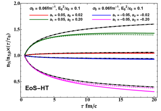
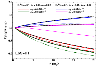
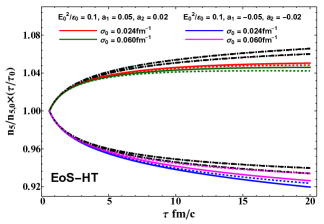
Figure 1: The proper time scaled electric field $E/E_{0}\times\left(\tau/\tau_{0}\right)$ and chiral charge density $n_{5}/n_{5,0}\times\left(\tau/\tau_{0}\right)$ computed with EoS-HC (14) as functions of proper time $\tau$ with different parameters $a_{1},a_{2},\sigma_{0}$. We have fixed $E_{0}^{2}/\varepsilon_{0}=0.1$. The colored solid, black dashed-dotted and colored dotted lines denote the results for solving the results from Eqs. (32, 33) numerically, analytic solutions (34, 41) and numerical results with a constant $\sigma$ derived in Ref. (Siddique:2019gqh, ; Wang:2020qpx, ), respectively.

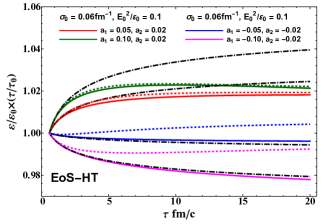
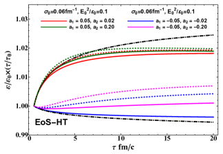
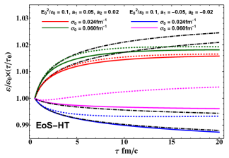
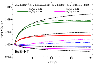
Figure 2: The proper time scaled energy density $\varepsilon/\varepsilon_{0}\times\left(\tau/\tau_{0}\right)^{1+c_{s}^{2}}$ computed with EoS-HT (14) as functions of proper time $\tau$ with different parameters $a_{1},a_{2},\sigma_{0}$ and $E_{0}^{2}/\varepsilon_{0}$. The colored solid, black dashed-dotted and colored dotted lines denote the results for solving the results from Eqs. (32, 33) numerically, analytic solutions (34, 41) and numerical results with a constant $\sigma$ derived in Ref. (Siddique:2019gqh, ; Wang:2020qpx, ), respectively.

From the numerical simulations in Ref. (Roy:2015coa, ), we find that the initial energy density of fluid $\varepsilon_{0}$ is much larger than the initial energy density of EM fields $\varepsilon_{0}\gg E_{0}^{2},B_{0}^{2},E_{0}B_{0}$. For simplicity, we consider $\mathcal{O}\left(\frac{E_{0}^{2}}{\varepsilon_{0}}\right)\sim\mathcal{O}(a_{1,2})\sim\mathcal{O}(\hbar)$. To the leading order of $\hbar$, we get the solutions for Eqs. (39),

$$x(\tau) = e^{m_{1}(\tilde{\tau}-1)}-a_{1}e^{m_{1}\tilde{\tau}}(1-c_{s}^{2})^{-1}[\mathcal{E}(n_{1},m_{1})-\tilde{\tau}^{-2c_{s}^{2}/(c_{s}^{2}-1)}\mathcal{E}(n_{1},m_{1}\tilde{\tau})],$$

$$y(\tau) = 1+a_{2}e^{-m_{1}}(1-c_{s}^{2})^{-1}[\mathcal{E}(1,-m_{1})-\mathcal{E}(1,-m_{1}\tilde{\tau})],$$

$$z(\tau) = 1-\frac{E_{0}^{2}}{\varepsilon_{0}}m_{1}e^{-2m_{1}}[\mathcal{E}(1,-2m_{1})-\mathcal{E}(1,-2m_{1}\tilde{\tau})]$$ (41)

$$+a_{1}\frac{E_{0}^{2}}{\varepsilon_{0}}e^{-m_{1}}(1-c_{s}^{2})^{-1}[\mathcal{E}(2n_{2},-m_{1})-\tilde{\tau}^{(1-3c_{s}^{2})/(c_{s}^{2}-1)}\mathcal{E}(2n_{2},-m_{1}\tilde{\tau})],$$

where

$$\mathcal{E}(n,m)\equiv\int_{1}^{\infty}dt\,t^{-n}e^{-mt},$$ (42)

is the generated exponential integral, and

$$n_{1} = \frac{1-3c_{s}^{2}}{1-c_{s}^{2}},$$

$$n_{2} = \frac{1-2c_{s}^{2}}{1-c_{s}^{2}},$$

$$m_{1} = -\frac{\sigma_{0}\tau_{0}}{1-c_{s}^{2}},$$

$$\tilde{\tau} = \left(\frac{\tau_{0}}{\tau}\right)^{c_{s}^{2}-1}.$$ (43)

Inserting the solutions for $x,y,z$ back into Eqs. (34), we can get the solutions for $E(\tau),n_{5}(\tau)$ and $\varepsilon(\tau)$.

In the order of $\hbar^{0}$, we find,

$$E(\tau) = E_{0}\left(\frac{\tau_{0}}{\tau}\right)x(\tau)\propto\frac{1}{\tau}e^{-\sigma(\tau)\tau},$$

$$n_{5}(\tau) = n_{5,0}\left(\frac{\tau_{0}}{\tau}\right)y(\tau)\propto\frac{\tau_{0}}{\tau},$$

$$\varepsilon(\tau) = \varepsilon_{0}\left(\frac{\tau_{0}}{\tau}\right)^{1+c_{s}^{2}}z(\tau)\propto\left(\frac{\tau_{0}}{\tau}\right)^{1+c_{s}^{2}},$$ (44)

which are consistent with the results in a ordinary MHD with finite electric conductivity in a Bjorken flow as discussed by Ref. (Siddique:2019gqh, ; Wang:2020qpx, ). We also find that,

$$\sigma(\tau)=\sigma_{0}\left[\frac{T(\tau)}{T(\tau_{0})}\right]\propto\left(\frac{\tau_{0}}{\tau}\right)^{c_{s}^{2}},$$ (45)

which decays with proper time. The numerical studies of $\sigma(\tau)$ in the evolution of QGP can also be found in Ref. (Zhang:2022lje, ; Wang:2021oqq, ).

Next, we present the above perturbative analytic solutions (34, 41) and the results for solving Eqs. (32) directly in a numerical way. We choose the $\tau_{0}=0.6\textrm{ fm/c}$ and the speed of sound $c_{s}^{2}=1/3$. The electric conductivity $\sigma$ are given by $\sigma\sim 5.8T/T_{c}\,\textrm{MeV}$ from lattice QCD (Aarts:2007wj, ; Ding:2010ga, ; Tuchin:2013ie, ) and $\sigma\sim 20-30\,\textrm{MeV}$ for $T\simeq 200\,\textrm{MeV}$ from the holographic QCD (Pu:2014cwa, ; Pu:2014fva, ). In this work, we choose the region of the initial electric conductivity $\sigma_{0}$ as $\sigma_{0}\sim 5-30\,\textrm{MeV}\simeq 0.025-0.15\ \mathrm{fm}^{-1}$.

From the solutions (41), the proper time scaled electric field $E/E_{0}\times\left(\tau/\tau_{0}\right)$ and chiral density $n_{5}/n_{5,0}\times\left(\tau/\tau_{0}\right)$ will not be sensitive to the $E_{0}^{2}/\varepsilon_{0}$. We have also confirmed it numerically. For simplicity, we fix $E_{0}^{2}/\varepsilon_{0}=0.1$ for the discussion on $E/E_{0}\times\left(\tau/\tau_{0}\right)$ and $n_{5}/n_{5,0}\times\left(\tau/\tau_{0}\right)$.

In left handed side of Fig. 1, we plot the proper time scaled electric field $E/E_{0}\times\left(\tau/\tau_{0}\right)$ as functions of the proper time $\tau$ with different sets of parameters $a_{1,2},\sigma_{0}$. The analytic solutions (34, 41) agree with the numerical results well. Note that our analytic solutions (41) for $E$ do not have the $a_{2}$ dependence and, therefore, it only matches the numerical results in small $|a_{2}|$ case.

Similar to Ref. (Siddique:2019gqh, ; Wang:2020qpx, ), we find that $E(\tau)$ decays faster when $a_{1}$ increases and $E/E_{0}$ can be negative at late time on condition that the initial $E$ and $B$ field are of the same orientation due to the competition between the anomalous conservation equation and Maxwell’s equations.

We can also compare the our results (solid or dashed-dotted liens) with temperature dependent $\sigma(\tau)$ to those with a constant $\sigma$ derived in Ref. (Siddique:2019gqh, ; Wang:2020qpx, ) (dotted lines). From Eq. (44) in the order of $\hbar^{0}$, $E(\tau)\sim\frac{1}{\tau}e^{-\sigma_{0}\tau_{0}^{c_{s}^{2}}\tau^{1-c_{s}^{2}}}\sim\frac{1}{\tau}e^{-\sigma_{0}\tau_{0}^{1/3}\tau^{2/3}}\leq\frac{1}{\tau}e^{-\sigma_{0}\tau_{0}}$ when $\tau\geq\tau_{0}$. It means that the $\sigma(\tau)$ will quicken up the decaying of $E(\tau)$. We can understand it in the following way. At late time limit, $\lim_{\tau\rightarrow\infty}\sigma(\tau)\rightarrow 0$, the fluid becomes dilute close to the vacuum and the EM fields decays much rapidity in the vacuum than in a medium. It is consistent with the results in Fig. 1. On the other hand, we also notice that when $a_{1,2}$ are negative, the $E/E_{0}\times\left(\tau/\tau_{0}\right)$ may increase when proper time grows. It corresponds to the cases that EM fields gain the energy from the medium.

In right handed side of Fig. 1, we present the proper time scaled chiral density $n_{5}/n_{5,0}\times\left(\tau/\tau_{0}\right)$ as functions of the proper time $\tau$ with different sets of parameters $a_{1},a_{2}$ and $\sigma_{0}$. Since our analytic solutions (41) for $n_{5}$ do not have the $a_{1}$ dependence, the analytic solutions for $n_{5}$ agree with the numerical results in small $|a_{1}|$ limit. We find that the proper time scaled chiral density is not sensitive to the $a_{1}$ and $\sigma_{0}$ at early proper time. It agrees with the analytic solutions (41). At late proper time, proper time scaled chiral density decreases with $a_{1}$ decreasing. We also observe that the proper time scaled chiral density increases when $a_{2}$ grows. The temperature dependent $\sigma(\tau)$ seems not to affect the evolution of $n_{5}$, which can also be found in the solutions (41).

In Figs. 2, we plot the proper time scaled energy density $\varepsilon/\varepsilon_{0}\times\left(\tau/\tau_{0}\right)^{1+c_{s}^{2}}$ as functions of the proper time $\tau$ with different sets of parameters $a_{1},a_{2},\sigma_{0}$ and $E_{0}^{2}/\varepsilon_{0}$.

As shown in Eqs. (41), our analytic solutions for $\varepsilon$ do not have $a_{2}$ dependence and it only corresponds to the small $|a_{2}|$ limit. On the other hand, we observe that our analytic solutions (41) for $\varepsilon$ matches the numerical results only at early proper time. It implies that the system is beyond the approximation for $\varepsilon$ in Eq. (36) at late proper time.

We observe that the proper time scaled energy density increases when $a_{1},a_{2},\sigma_{0},E_{0}^{2}/\varepsilon_{0}$ increases. When $a_{1},a_{2},\sigma_{0},E_{0}^{2}/\varepsilon_{0}$ is large enough, the proper time scaled energy density can increase with proper time. It corresponds that the medium gains the energy from the EM fields, which is also found in the ideal MHD with a background magnetic field (Roy:2015kma, ; Pu:2016ayh, ). In the comparison with the case of constant $\sigma_{0}$, we find that the temperature dependent $\sigma(\tau)$ enhances the decaying of energy density.

In this section, we have solved the MHD with the temperature dependent $\sigma(\tau$) in Eq. (15) and EoS-HT (14). We present both the analytic solutions (41) up to the $\mathcal{O}(\hbar)$ and the numerical results.

V Solutions in high chiral chemical potential limit

In this section, we solve the simplified differential equations (26, 27) with the EoS-HC (16) and temperature and energy density dependent conductivity (17).

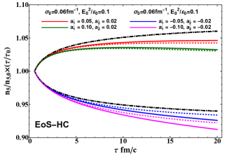
Figure 3: The proper time scaled electric field $E/E_{0}\times\left(\tau/\tau_{0}\right)$ and chiral density $n_{5}/n_{5,0}\times\left(\tau/\tau_{0}\right)$ computed with EoS-HC (16) as functions of proper time $\tau$ with different parameters $a_{1},a_{2},\sigma_{0}$. For simplicity, we fix $E_{0}^{2}/\varepsilon_{0}=0.1$. The colored solid, black dashed-dotted and colored dotted lines denote the results for solving the results from Eqs. (32, 33) numerically, analytic solutions (34, 49) and numerical results with a constant $\sigma$ derived in Ref. (Siddique:2019gqh, ; Wang:2020qpx, ), respectively.

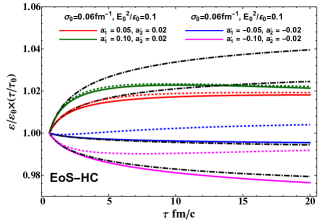
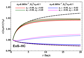
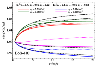
Figure 4: The proper time scaled energy density $\varepsilon/\varepsilon_{0}\times\left(\tau/\tau_{0}\right)^{1+c_{s}^{2}}$ computed with EoS-HC (16) as functions of proper time $\tau$ with different parameters $a_{1},a_{2},\sigma_{0}$ and $E_{0}^{2}/\varepsilon_{0}$. The colored solid, black dashed-dotted and colored dotted lines denote the results for solving the results from Eqs. (32, 33) numerically, analytic solutions (34, 49) and numerical results with a constant $\sigma$ derived in Ref. (Siddique:2019gqh, ; Wang:2020qpx, ), respectively.

Following the same method in the previous section, we can get the Eqs. (32, 33, 34, 35). The conductivity (17) becomes,

$$\sigma=\sigma_{0}\left(\frac{\tau_{0}}{\tau}\right)^{\frac{2}{3}-c_{s}^{2}}y^{2/3}\cdot z^{-c_{s}^{2}/(1+c_{s}^{2})}.$$ (46)

Using variables $x,y,z$, Eqs. (33) becomes,

$$\frac{d}{d\tau}x = -\sigma_{0}\left(\frac{\tau_{0}}{\tau}\right)^{\frac{2}{3}-c_{s}^{2}}xy^{2/3}\cdot z^{-c_{s}^{2}/(1+c_{s}^{2})}-\frac{a_{1}^{\prime}}{\tau_{0}}\left(\frac{\tau_{0}}{\tau}\right)^{1/3}y^{1/3},$$

$$\frac{d}{d\tau}y = a_{2}^{\prime}\frac{x}{\tau},$$

$$\frac{d}{d\tau}z = \frac{E_{0}^{2}}{\varepsilon_{0}}\sigma_{0}\left(\frac{\tau_{0}}{\tau}\right)^{\frac{5}{3}-2c_{s}^{2}}x^{2}y^{2/3}z^{-c_{s}^{2}/(1+c_{s}^{2})}+\frac{a_{1}^{\prime}}{\tau_{0}}\left(\frac{E_{0}^{2}}{\varepsilon_{0}}\right)\left(\frac{\tau_{0}}{\tau}\right)^{\frac{4}{3}-c_{s}^{2}}xy^{1/3},$$ (47)

where $x(\tau_{0})=y(\tau_{0})=z(\tau_{0})=1$, and dimensionless constants $a_{1}^{\prime}$, $a_{2}^{\prime}$ read

$$a_{1}^{\prime} = eC\chi\left(\frac{n_{5,0}}{a}\right)^{1/3}\frac{B_{0}}{E_{0}}\tau_{0},$$

$$a_{2}^{\prime} = e^{2}C\chi\frac{E_{0}B_{0}}{n_{5,0}}\tau_{0}.$$ (48)

We follow the same power counting in Sec.IV, i.e. $\mathcal{O}\left(\frac{E_{0}^{2}}{\varepsilon_{0}}\right)\sim\mathcal{O}(a_{1,2}^{\prime})\sim\mathcal{O}(\hbar)$ and derive the analytic solutions up to the order of $\hbar$,

$$x(\tau) = e^{m_{1}^{\prime}(\tilde{\tau}^{\prime}-1)}+\frac{3}{2}a_{1}e^{m_{1}^{\prime}\tilde{\tau}^{\prime}}(n_{1}^{\prime}-1)[\mathcal{E}(n_{1}^{\prime},m_{1}^{\prime})-\tilde{\tau}^{\prime 2/(1+3c_{s}^{2})}\mathcal{E}(n_{1}^{\prime},m_{1}^{\prime}\tilde{\tau}^{\prime})],$$

$$y(\tau) = 1-\frac{3}{2}a_{2}e^{-m_{1}^{\prime}}(n_{1}^{\prime}-1)[\mathcal{E}(1,-m_{1}^{\prime})-\mathcal{E}(1,-m_{1}^{\prime}\tilde{\tau}^{\prime})],$$

$$z(\tau) = 1-m_{1}^{\prime}\frac{E_{0}^{2}}{\varepsilon_{0}}e^{-2m_{1}^{\prime}}[\mathcal{E}(-2n_{1}^{\prime}+1,-2m_{1}^{\prime})-\tilde{\tau}^{\prime 2n_{1}^{\prime}}\mathcal{E}(-2n_{1}^{\prime}+1,-2m_{1}^{\prime}\tilde{\tau}^{\prime})]$$ (49)

$$-\frac{3}{2}a_{1}\left(\frac{E_{0}^{2}}{\varepsilon_{0}}\right)e^{-m_{1}^{\prime}}(n_{1}^{\prime}-1)[\mathcal{E}(-n_{1}^{\prime}+1,-m_{1}^{\prime})-\tilde{\tau}^{\prime n_{1}^{\prime}}\mathcal{E}(-n_{1}^{\prime}+1,-m_{1}^{\prime}\tilde{\tau}^{\prime})].$$

where we introduce

$$n_{1}^{\prime} = \frac{-1+3c_{s}^{2}}{1+3c_{s}^{2}},$$

$$m_{1}^{\prime} = -\frac{\sigma_{0}\tau_{0}}{\frac{1}{3}+c_{s}^{2}},$$

$$\tilde{\tau}^{\prime} = \left(\frac{\tau_{0}}{\tau}\right)^{-\frac{1}{3}-c_{s}^{2}}.$$ (50)

For the numerical calculations, we choose the $\tau_{0}=0.6\textrm{ fm/c}$ and the speed of sound $c_{s}^{2}=1/3$. Meanwhile, we fix $E_{0}^{2}/\varepsilon_{0}=0.1$ for the discussion on $E/E_{0}\times\left(\tau/\tau_{0}\right)$ and $n_{5}/n_{5,0}\times\left(\tau/\tau_{0}\right)$ again.

In Figs. 3, we plot the proper time scaled electric field $E/E_{0}\times\left(\tau/\tau_{0}\right)$, chiral density $n_{5}/n_{5,0}\times\left(\tau/\tau_{0}\right)$ as functions of the proper time $\tau$ with different parameters $a_{1}^{\prime},a_{2}^{\prime}$ and $\sigma_{0}$. Interesting, in the comparison with Fig. 1, the proper time scaled electric field in small $|a_{2}^{\prime}|$ cases and chiral density, computed with EoS-HC, seem to be close the those computed with EoS-HT when we choose $a_{1}=a_{1}^{\prime}$ and $a_{2}=a_{2}^{\prime}$. It means that the evolution of electric fields in the small $|a_{2}^{\prime}|$ cases and chiral density are not sensitive to the EoS.

Different with constant electric conductivity case in Ref. (Siddique:2019gqh, ; Wang:2020qpx, ) (colored dotted lines in Fig. 3), the temperature and energy density dependent $\sigma(\tau)$ with EoS-HC will slow down the decaying of electric fields when $a_{2}^{\prime}<0$. Such behavior is also also insensitive to the $|a_{2}^{\prime}|$ when $a_{2}^{\prime}<0$.

In Fig. 4, we present the proper time scaled energy density $\varepsilon/\varepsilon_{0}\times\left(\tau/\tau_{0}\right)^{1+c_{s}^{2}}$ as functions of the proper time $\tau$ with different parameters $a_{1}^{\prime},a_{2}^{\prime},\sigma_{0}$ and $E_{0}^{2}/\varepsilon_{0}$. We observe the similarity in small $|a_{2}^{\prime}|$ cases between the figures in Fig. 4 and in Fig. 2. When $a_{2}^{\prime}<0$, the evolution of energy density is insensitive to the $|a_{2}^{\prime}|$. The temperature and energy density dependent electric conductivity $\sigma(\tau)$ will accelerate the decaying of energy density when $a_{2}^{\prime}<0$. Combining with the results in Fig. 3, it implies that the temperature and energy density dependent electric conductivity $\sigma(\tau)$ helps the electric fields gain the energy from the medium.

In this section, we have solved the MHD with the temperature and energy density dependent $\sigma(\tau$) in Eq. (17) and EoS-HC. We present both the analytic solutions (49) up to the $\mathcal{O}(\hbar)$ and the numerical results.

VI Splitting of global polarization for $\Lambda$ and $\overline{\Lambda}$ hyperons induced by magnetic fields

In this section, we implement the results for relativistic MHD to the global polarization of $\Lambda$ and $\overline{\Lambda}$ hyperons in the relativistic heavy ion collisions.

The polarization pesudo-vector is given by the modified Cooper-Frye formula (Becattini:2013fla, ; Fang:2016uds, ),

$$\mathcal{S}^{\mu}({\bf p})=\frac{\int d\Sigma\cdot p\mathcal{J}_{5}^{\mu}(p,X)}{2m_{\Lambda}\int d\Sigma\cdot\mathcal{N}(p,X)},$$ (51)

where $m_{\Lambda}$ is the mass of $\Lambda$ hyperon, $\Sigma$ is the freeze out hypersurface, $\mathcal{J}_{5}^{\mu}(p,X)$ and $\mathcal{N}^{\mu}(p,x)$ are axial and vector components of Wigner functions in phase space. By inserting the general solutions in Wigner functions (Gao:2012ix, ; Chen:2012ca, ; Hidaka:2016yjf, ; Hidaka:2017auj, ; Hidaka:2018ekt, ; Hidaka:2022dmn, ; Fang:2022ttm, ), the polarization vector $\mathcal{S}^{\mu}$ in Eq. (51) can be divide as several different parts (Hidaka:2017auj, ; Yi:2021ryh, ; Yi:2021unq, ),

$$\mathcal{S}^{\mu}(\mathbf{p}) = \mathcal{S}_{\textrm{thermal}}^{\mu}(\mathbf{p})+\mathcal{S}_{\textrm{shear}}^{\mu}(\mathbf{p})+\mathcal{S}_{\textrm{accT}}^{\mu}(\mathbf{p})+\mathcal{S}_{\textrm{chemical}}^{\mu}(\mathbf{p})+\mathcal{S}_{\textrm{EB}}^{\mu}(\mathbf{p}),$$ (52)

where

$$\mathcal{S}_{\textrm{thermal}}^{\mu}(\mathbf{p}) = \int d\Sigma^{\sigma}F_{\sigma}\epsilon^{\mu\nu\alpha\beta}p_{\nu}\partial_{\alpha}\frac{u_{\beta}}{T},$$

$$\mathcal{S}_{\textrm{shear}}^{\mu}(\mathbf{p}) = \int d\Sigma^{\sigma}F_{\sigma}\frac{\epsilon^{\mu\nu\alpha\beta}p_{\nu}u_{\beta}}{(u\cdot p)T}$$

$$\times p^{\rho}[\partial_{\rho}u_{\alpha}+\partial_{\alpha}u_{\rho}-u_{\rho}(u\cdot\partial)u_{\alpha}],$$

$$\mathcal{S}_{\textrm{accT}}^{\mu}(\mathbf{p}) = -\int d\Sigma^{\sigma}F_{\sigma}\frac{\epsilon^{\mu\nu\alpha\beta}p_{\nu}u_{\alpha}}{T}\left[(u\cdot\partial)u_{\beta}-\frac{\partial_{\beta}T}{T}\right],$$

$$\mathcal{S}_{\textrm{chemical}}^{\mu}(\mathbf{p}) = 2\int d\Sigma^{\sigma}F_{\sigma}\frac{1}{(u\cdot p)}\epsilon^{\mu\nu\alpha\beta}p_{\alpha}u_{\beta}\partial_{\nu}\frac{\mu_{B}}{T},$$

$$\mathcal{S}_{\textrm{EB}}^{\mu}(\mathbf{p}) = 2\int d\Sigma^{\sigma}F_{\sigma}\left[\frac{\epsilon^{\mu\nu\alpha\beta}p_{\alpha}u_{\beta}E_{\nu}}{(u\cdot p)T}+\frac{B^{\mu}}{T}\right],$$ (53)

with

$$F^{\mu} = \frac{\hbar}{8m_{\Lambda}\Phi(\mathbf{p})}p^{\mu}f_{eq}(1-f_{eq}),$$

$$\Phi(\mathbf{p}) = \int d\Sigma^{\mu}p_{\mu}f_{eq}.$$ (54)

where $\Phi(\mathbf{p})=\int d\Sigma^{\mu}p_{\mu}f_{eq}(x,p)$ is the particle number density at freeze out hypersurface, $\mu_{B}$ is the baryon chemical potential and $f_{eq}$ is assumed as the standard Fermi-Dirac distribution function. The $\mathcal{S}_{\textrm{thermal}}^{\mu}(\mathbf{p}),\mathcal{S}_{\textrm{shear}}^{\mu}(\mathbf{p}),\mathcal{S}_{\textrm{accT}}^{\mu}(\mathbf{p})$ for $\Lambda$ hyperons are the same as those for $\overline{\Lambda}$ hyperons. While, due to the difference in charge and baryon number, $\mathcal{S}_{\textrm{chemical}}^{\mu}(\mathbf{p})$ and $\mathcal{S}_{\textrm{EB}}^{\mu}(\mathbf{p})$ flip their sign when we change $\Lambda$ to $\overline{\Lambda}$ hyperons. Therefore, the gradient of $\mu_{B}/T$ and EM fields can lead to the splitting of global polarization for $\Lambda$ and $\overline{\Lambda}$ hyperons.

In order to compare with experiments, we need to transform the polarization pseudo vector in the rest frame of $\Lambda$ and $\overline{\Lambda}$, named $\vec{P}^{*}(\mathbf{p})$

$$\vec{P}^{*}(\mathbf{p})=\vec{P}(\mathbf{p})-\frac{\vec{P}(\mathbf{p})\cdot\vec{p}}{p^{0}(p^{0}+m)}\vec{p},$$ (55)

where

$$P^{\mu}(\mathbf{p})\equiv\frac{1}{s}\mathcal{S}^{\mu}(\mathbf{p}),$$ (56)

with $s=1/2$ being the spin of the particle. Finally, the local polarization is given by the averaging over momentum and rapidity as follows,

$$\langle\vec{P}(\phi_{p})\rangle=\frac{\int_{y_{\text{min}}}^{y_{\text{max}}}dy\int_{p_{T\text{min}}}^{p_{T\text{max}}}p_{T}dp_{T}[\Phi(\mathbf{p})\vec{P}^{*}(\mathbf{p})]}{\int_{y_{\text{min}}}^{y_{\text{max}}}dy\int_{p_{T\text{min}}}^{p_{T\text{max}}}p_{T}dp_{T}\Phi(\mathbf{p})},$$ (57)

where $\phi_{p}$ is the azimuthal angle.

In this work, we concentrate on the splitting induced by the magnetic fields. From Eq. (53), we introduce

$$\Delta\mathcal{P}=\mathcal{P}_{\Lambda}-\mathcal{P}_{\overline{\Lambda}},$$ (58)

where $\mathcal{P}_{\Lambda}$ and $\mathcal{P}_{\overline{\Lambda}}$ are the integration of local polarization (57) alone the out-of-plane direction over the $\phi_{p}$. Taking $1-f_{eq}\simeq 1$ in Eqs. (53), the $\Delta\mathcal{P}$ induced by the magnetic fields is given by, $\Delta\mathcal{P}_{\textrm{EB}}\propto B^{y}/(m_{\Lambda}T)$. Recalling the definition spin magnetic moment, following Ref. (Muller:2018ibh, ), $\Delta\mathcal{P}$ induced by magnetic fields is estimated as

$$\Delta\mathcal{P}_{\textrm{EB}}\approx 2\frac{\mu_{\Lambda}}{T}\overline{B},$$ (59)

where $\mu_{\Lambda}=-0.613\mu_{N}$ is the spin magnetic moment for $\Lambda$ hyperons. In the Ref. (Muller:2018ibh, ), $\overline{B}$ is averaged the magnetic field. Also see other related theoretical studies on the splitting of polarization induced by EM fields (Guo:2019joy, ; Buzzegoli:2022qrr, ; Xu:2022hql, ).

Next, we will evaluate the $\Delta\mathcal{P}_{\textrm{EB}}$ in the framework of relativistic magnetohydrodynamics. Recalling the expression in Eq. (57), since the polarization pseudo vector is computed near the freeze out surface, it is natural for us to choose the $B^{y}(\tau_{f})$ with $\tau_{f}$ being the proper time for the chemical freeze out instead of the averaged $\overline{B}$. For a given collision energy, we choose the maximum value of space-averaged initial magnetic fields in different impact parameters, which is computed by Ref. (Siddique:2021smf, ). The initial proper time is chosen as $\tau_{0}\simeq 0.6$fm/c. The evolution of magnetic fields is given by Eq. (31), which is also found in ideal MHD Ref. (Pu:2016ayh, ; Roy:2015kma, ; Pu:2016bxy, ; Pu:2016rdq, ). For simplicity, we choose the $\tau_{f}=10$fm/c for all collision energies. The temperature for the chemical freeze out is followed by the experimental studies in Ref. (STAR:2021iop, ). We summarize these parameters in different collision energies in Tab. 1.

Table 1: Collision energies, temperature given by Ref. (STAR:2021iop, ) , the initial space-averaged magnetic fields from Ref. (Siddique:2021smf, ), the magnetic fields estimated by Eq. (31) with $\tau_{f}=10$fm/c.

$\sqrt{s_{NN}}$ (GeV)	$7.7$	$11.5$	$27$	$39$	$62.4$	$200$
$T$ (MeV)	$144.3$	$149.4$	$155.0$	$156.4$	$160.3$	$164.3$
space-averaged $eB(\tau_{0})/m_{\pi}^{2}$	$9.1\times 10^{-2}$	$1.7\times 10^{-1}$	$4.5\times 10^{-1}$	$4.5\times 10^{-1}$	$3.2\times 10^{-1}$	$5.6\times 10^{-2}$
$eB(\tau_{f})/m_{\pi}^{2}$	$5.5\times 10^{-3}$	$1.0\times 10^{-2}$	$2.7\times 10^{-2}$	$2.7\times 10^{-2}$	$1.9\times 10^{-2}$	$3.3\times 10^{-3}$

Figure 5: The difference of the global polarization between $\Lambda$ and $\overline{\Lambda}$ hyperons in different collision energies. The triangle points are derived from STAR measurements (STAR:2017ckg, ; STAR:2018gyt, ). The filled circle points denotes the estimation from Eqs. (59) where the initial magnetic fields at $\tau_{0}=0.6$fm/c are given by Ref. (Siddique:2021smf, ) and the evolution of magnetic fields are given by Eq. (31) with final time $\tau_{f}=10$fm/c.

In Fig. 5, we plot the the splitting of the global polarization for $\Lambda$ and $\overline{\Lambda}$ hyperons, and compare our estimation from Eq. (59) with the data from STAR measurements (STAR:2017ckg, ; STAR:2018gyt, ) at $\sqrt{s_{NN}}=7.7,11.5,27,39,62.4,200\ \text{GeV}$ collisions. We find that the $\Delta\mathcal{P}_{\textrm{EB}}$ computed from our framework agrees with the data expect the results at $\sqrt{s_{NN}}=7.7$ GeV. Roughly speaking, in the high energy collisions, the quark pairs are generated from the vacuum and therefore, the net baryon number and baryon chemical potential are approximately vanishing. The splitting induced by EM fields may dominate in the global polarization of $\Lambda$ and $\overline{\Lambda}$ hyperons in the high energy region. On the other hand, the collisions in low energy region, the net baryon density is not negligible and will play a crucial role to the global and local polarization, e.g. see Ref. (Ryu:2021lnx, ) and the discussions on the simulations for spin Hall effects in heavy ion collisions (Fu:2022myl, ; Wu:2022mkr, ). Our results indicates that the magnetic fields may be not strong enough to cause such huge splitting of global polarization in low energy region. It implies that the contributions from $\nabla\mu_{B}/T$ may dominate the splitting of global polarization in low energy collisions (Ryu:2021lnx, ; Wu:2022mkr, ).

VII Summary

We have derived the solutions of the relativistic anomalous magnetohydronamic with longitudinal Bjorken boost invariance and transverse electromagnetic fields in the presence of temperature or energy density dependent electric conductivity.

After a short review on the anomalous MHD in Sec. II, we simplify the energy-momentum and charge currents conversation equations coupled to the Maxwell’s equations. To close the system, we introduce two kinds of EoS, i.e. EoS-HT (14) and EoS-HC (16) correspond to the high temperature and high chiral chemical potential limits, respectively. The electric conductivity is also parameterized as Eqs. (15) and (17) for the EoS-HT and EoS-HC, respectively. We assume that the initial conditions for the system is a Bjorken velocity (24) with initial EM fields in Eq. (25). After some calculations, we confirm that the Bjorken boost invariance holds during the evolution. The main differential equations reduce to Eqs. (26, 27).

Next, in Sec. 15, we derive the perturbative analytic solutions (34, 41) up to the order of $\hbar$ for the simplified differential equations (26, 27) with the EoS-HT (14) and temperature dependent conductivity (15). We present the numerical solutions for electric fields, chiral density and energy density in Figs.1, 2. We find that the temperature dependent $\sigma(\tau)$ will quicken up the decaying of electric fields. While, the decaying of chiral density seems not to be sensitive to the $\sigma(\tau)$.

Similarly, we derive the perturbative analytic solutions (34, 49) up to the order of $\hbar$ with the EoS-HT (16) and temperature dependent conductivity (17). The numerical results for the proper time scaled electric fields, chiral density and energy density are shown in Figs. 3, 4. We find that the decaying of electric fields and energy density in the small $|a_{2}^{\prime}|$ limit and chiral density seem not be affected by the EoS when we choose $a_{1}=a_{1}^{\prime}$ and $a_{2}=a_{2}^{\prime}$. On the other hand, when $a_{2}^{\prime}<0$, temperature and energy density dependent electric conductivity $\sigma(\tau)$ will slow down or accelerate the decaying of electric fields or energy density, respectively.

At last, we implement the results for relativistic MHD to the global polarization of $\Lambda$ and $\overline{\Lambda}$ hyperons in the relativistic heavy ion collisions in Sec. VI. The splitting of global polarization for $\Lambda$ and $\overline{\Lambda}$ hyperons is estimated by Eq. (59). In Fig. 5, we plot the the splitting of the global polarization for $\Lambda$ and $\overline{\Lambda}$ hyperons, and compare our estimation from Eq. (59) with the data from STAR measurements at $\sqrt{s_{NN}}=7.7,11.5,27,39,62.4,200\ \text{GeV}$ collisions. The $\Delta\mathcal{P}_{\textrm{EB}}$ computed from our framework agrees with the data in both high and intermediate collisions energies and fails at $\sqrt{s_{NN}}=7.7$ GeV. It implies that the contributions from other sources, e.g. $\nabla\mu_{B}/T$, may dominate the splitting of global polarization in low energy collisions.

- (1) V. Skokov, A. Y. Illarionov, and V. Toneev, Int. J. Mod. Phys. A 24, 5925 (2009), 0907.1396.
- (2) A. Bzdak and V. Skokov, Phys. Lett. B 710, 171 (2012), 1111.1949.
- (3) W.-T. Deng and X.-G. Huang, Phys. Rev. C 85, 044907 (2012), 1201.5108.
- (4) V. Roy and S. Pu, Phys. Rev. C92, 064902 (2015), 1508.03761.
- (5) A. Vilenkin, Phys. Rev. D22, 3080 (1980).
- (6) D. Kharzeev and A. Zhitnitsky, Nucl. Phys. A 797, 67 (2007), 0706.1026.
- (7) D. E. Kharzeev, L. D. McLerran, and H. J. Warringa, Nuclear Physics A 803, 227 (2008).
- (8) K. Fukushima, D. E. Kharzeev, and H. J. Warringa, Phys. Rev. D 78, 074033 (2008), 0808.3382.
- (9) Y. Aghababaie and C. P. Burgess, Phys. Rev. D 70, 085003 (2004), hep-th/0304066.
- (10) D. E. Kharzeev and H.-U. Yee, Phys. Rev. D 83, 085007 (2011), 1012.6026.
- (11) Y. Burnier, D. E. Kharzeev, J. Liao, and H.-U. Yee, Phys. Rev. Lett. 107, 052303 (2011), 1103.1307.
- (12) X.-G. Huang and J. Liao, Phys. Rev. Lett. 110, 232302 (2013), 1303.7192.
- (13) S. Pu, S.-Y. Wu, and D.-L. Yang, Phys. Rev. D89, 085024 (2014), 1401.6972.
- (14) Y. Jiang, X.-G. Huang, and J. Liao, Phys. Rev. D 91, 045001 (2015), 1409.6395.
- (15) S. Pu, S.-Y. Wu, and D.-L. Yang, Phys. Rev. D91, 025011 (2015), 1407.3168.
- (16) J.-W. Chen, T. Ishii, S. Pu, and N. Yamamoto, Phys. Rev. D 93, 125023 (2016), 1603.03620.
- (17) E. V. Gorbar et al., Phys. Rev. D 93, 105028 (2016), 1603.03442.
- (18) E. V. Gorbar, V. A. Miransky, I. A. Shovkovy, and P. O. Sukhachov, Phys. Rev. B 95, 115202 (2017), 1611.05470.
- (19) E. V. Gorbar, V. A. Miransky, I. A. Shovkovy, and P. O. Sukhachov, Phys. Rev. Lett. 118, 127601 (2017), 1610.07625.
- (20) E. V. Gorbar, V. A. Miransky, I. A. Shovkovy, and P. O. Sukhachov, Phys. Rev. B 95, 205141 (2017), 1702.02950.
- (21) K. Fukushima, D. E. Kharzeev, and H. J. Warringa, Phys. Rev. Lett. 104, 212001 (2010), 1002.2495.
- (22) H. J. Warringa, Phys. Rev. D 86, 085029 (2012), 1205.5679.
- (23) P. Copinger, K. Fukushima, and S. Pu, Phys. Rev. Lett. 121, 261602 (2018), 1807.04416.
- (24) P. Copinger and S. Pu, Int. J. Mod. Phys. A 35, 2030015 (2020), 2008.03635.
- (25) P. Copinger and S. Pu, Phys. Rev. D 105, 116014 (2022), 2203.00847.
- (26) D. E. Kharzeev, K. Landsteiner, A. Schmitt, and H.-U. Yee, Lect. Notes Phys. 871, 1 (2013), 1211.6245.
- (27) D. E. Kharzeev, J. Liao, S. A. Voloshin, and G. Wang, Prog. Part. Nucl. Phys. 88, 1 (2016), 1511.04050.
- (28) J. Liao, Pramana 84, 901 (2015), 1401.2500.
- (29) V. A. Miransky and I. A. Shovkovy, Phys. Rept. 576, 1 (2015), 1503.00732.
- (30) X.-G. Huang, Rept. Prog. Phys. 79, 076302 (2016), 1509.04073.
- (31) K. Fukushima, Prog. Part. Nucl. Phys. 107, 167 (2019), 1812.08886.
- (32) A. Bzdak et al., (2019), 1906.00936.
- (33) J. Zhao and F. Wang, Prog. Part. Nucl. Phys. 107, 200 (2019), 1906.11413.
- (34) J.-H. Gao, G.-L. Ma, S. Pu, and Q. Wang, Nucl. Sci. Tech. 31, 90 (2020), 2005.10432.
- (35) I. A. Shovkovy, (2021), 2111.11416.
- (36) J.-H. Gao, Z.-T. Liang, S. Pu, Q. Wang, and X.-N. Wang, Phys. Rev. Lett. 109, 232301 (2012), 1203.0725.
- (37) D. T. Son and N. Yamamoto, Phys. Rev. D 87, 085016 (2013), 1210.8158.
- (38) J.-W. Chen, S. Pu, Q. Wang, and X.-N. Wang, Phys. Rev. Lett. 110, 262301 (2013), 1210.8312.
- (39) M. A. Stephanov and Y. Yin, Phys. Rev. Lett. 109, 162001 (2012), 1207.0747.
- (40) C. Manuel and J. M. Torres-Rincon, Phys. Rev. D 89, 096002 (2014), 1312.1158.
- (41) J.-W. Chen, J.-H. Gao, J. Liu, S. Pu, and Q. Wang, Phys. Rev. D 88, 074003 (2013), 1305.1835.
- (42) C. Manuel and J. M. Torres-Rincon, Phys. Rev. D 90, 076007 (2014), 1404.6409.
- (43) J.-Y. Chen, D. T. Son, M. A. Stephanov, H.-U. Yee, and Y. Yin, Phys. Rev. Lett. 113, 182302 (2014), 1404.5963.
- (44) J.-Y. Chen, D. T. Son, and M. A. Stephanov, Phys. Rev. Lett. 115, 021601 (2015), 1502.06966.
- (45) Y. Hidaka, S. Pu, and D.-L. Yang, Phys. Rev. D 95, 091901 (2017), 1612.04630.
- (46) N. Mueller and R. Venugopalan, Phys. Rev. D 97, 051901 (2018), 1701.03331.
- (47) Y. Hidaka, S. Pu, and D.-L. Yang, Phys. Rev. D 97, 016004 (2018), 1710.00278.
- (48) J.-h. Gao, S. Pu, and Q. Wang, Phys. Rev. D 96, 016002 (2017), 1704.00244.
- (49) Y.-C. Liu, L.-L. Gao, K. Mameda, and X.-G. Huang, Phys. Rev. D 99, 085014 (2019), 1812.10127.
- (50) Y. Hidaka and D.-L. Yang, Phys. Rev. D 98, 016012 (2018), 1801.08253.
- (51) A. Huang, S. Shi, Y. Jiang, J. Liao, and P. Zhuang, Phys. Rev. D 98, 036010 (2018), 1801.03640.
- (52) Y. Hidaka, S. Pu, and D.-L. Yang, Nucl. Phys. A 982, 547 (2019), 1807.05018.
- (53) J.-H. Gao, Z.-T. Liang, Q. Wang, and X.-N. Wang, Phys. Rev. D 98, 036019 (2018), 1802.06216.
- (54) J.-H. Gao and Z.-T. Liang, Phys. Rev. D 100, 056021 (2019), 1902.06510.
- (55) Z. Wang, X. Guo, S. Shi, and P. Zhuang, Phys. Rev. D 100, 014015 (2019), 1903.03461.
- (56) S. Li and H.-U. Yee, Phys. Rev. D 100, 056022 (2019), 1905.10463.
- (57) N. Weickgenannt, X.-L. Sheng, E. Speranza, Q. Wang, and D. H. Rischke, Phys. Rev. D 100, 056018 (2019), 1902.06513.
- (58) K. Hattori, Y. Hidaka, and D.-L. Yang, Phys. Rev. D 100, 096011 (2019), 1903.01653.
- (59) S. Lin and A. Shukla, JHEP 06, 060 (2019), 1901.01528.
- (60) S. Lin and L. Yang, Phys. Rev. D 101, 034006 (2020), 1909.11514.
- (61) J.-H. Gao, Z.-T. Liang, and Q. Wang, Phys. Rev. D 101, 096015 (2020), 1910.11060.
- (62) N. Weickgenannt, E. Speranza, X.-l. Sheng, Q. Wang, and D. H. Rischke, Phys. Rev. Lett. 127, 052301 (2021), 2005.01506.
- (63) N. Weickgenannt, X.-L. Sheng, E. Speranza, Q. Wang, and D. H. Rischke, Nucl. Phys. A 1005, 121963 (2021), 2001.11862.
- (64) Y.-C. Liu, K. Mameda, and X.-G. Huang, Chin. Phys. C 44, 094101 (2020), 2002.03753, [Erratum: Chin.Phys.C 45, 089001 (2021)].
- (65) A. Huang et al., Phys. Rev. D 103, 056025 (2021), 2007.02858.
- (66) N. Yamamoto and D.-L. Yang, Astrophys. J. 895, 56 (2020), 2002.11348.
- (67) D.-L. Yang, K. Hattori, and Y. Hidaka, JHEP 07, 070 (2020), 2002.02612.
- (68) Z. Wang and P. Zhuang, (2021), 2105.00915.
- (69) X.-L. Sheng, N. Weickgenannt, E. Speranza, D. H. Rischke, and Q. Wang, Phys. Rev. D 104, 016029 (2021), 2103.10636.
- (70) X.-L. Luo and J.-H. Gao, JHEP 11, 115 (2021), 2107.11709.
- (71) N. Weickgenannt, E. Speranza, X.-l. Sheng, Q. Wang, and D. H. Rischke, Phys. Rev. D 104, 016022 (2021), 2103.04896.
- (72) Y. Hidaka, S. Pu, Q. Wang, and D.-L. Yang, (2022), 2201.07644.
- (73) S. Fang, S. Pu, and D.-L. Yang, (2022), 2204.11519.
- (74) J.-H. Gao, Z.-T. Liang, and Q. Wang, Int. J. Mod. Phys. A 36, 2130001 (2021), 2011.02629.
- (75) STAR, B. I. Abelev et al., Phys. Rev. Lett. 103, 251601 (2009), 0909.1739.
- (76) STAR, B. I. Abelev et al., Phys. Rev. C 81, 054908 (2010), 0909.1717.
- (77) STAR, G. Wang, Nucl. Phys. A 904-905, 248c (2013), 1210.5498.
- (78) STAR, L. Adamczyk et al., Phys. Rev. C 88, 064911 (2013), 1302.3802.
- (79) STAR, L. Adamczyk et al., Phys. Rev. C 89, 044908 (2014), 1303.0901.
- (80) STAR, L. Adamczyk et al., Phys. Rev. Lett. 113, 052302 (2014), 1404.1433.
- (81) STAR, P. Tribedy, Nucl. Phys. A 967, 740 (2017), 1704.03845.
- (82) STAR, J. Adam et al., Phys. Lett. B 798, 134975 (2019), 1906.03373.
- (83) ALICE, B. Abelev et al., Phys. Rev. Lett. 110, 012301 (2013), 1207.0900.
- (84) CMS, V. Khachatryan et al., Phys. Rev. Lett. 118, 122301 (2017), 1610.00263.
- (85) CMS, A. M. Sirunyan et al., Phys. Rev. C 97, 044912 (2018), 1708.01602.
- (86) S. Pratt, S. Schlichting, and S. Gavin, Phys. Rev. C 84, 024909 (2011), 1011.6053.
- (87) A. Bzdak, V. Koch, and J. Liao, Lect. Notes Phys. 871, 503 (2013), 1207.7327.
- (88) N. N. Ajitanand, R. A. Lacey, A. Taranenko, and J. M. Alexander, Phys. Rev. C 83, 011901 (2011), 1009.5624.
- (89) N. Magdy, S. Shi, J. Liao, N. Ajitanand, and R. A. Lacey, Phys. Rev. C 97, 061901 (2018), 1710.01717.
- (90) A. H. Tang, Chin. Phys. C 44, 054101 (2020), 1903.04622.
- (91) S. Schlichting and S. Pratt, Phys. Rev. C 83, 014913 (2011), 1009.4283.
- (92) H.-J. Xu et al., Phys. Rev. Lett. 121, 022301 (2018), 1710.03086.
- (93) H.-j. Xu, J. Zhao, Y. Feng, and F. Wang, Nucl. Phys. A 1005, 121770 (2021), 2002.05220.
- (94) S. A. Voloshin, Phys. Rev. Lett. 105, 172301 (2010), 1006.1020.
- (95) STAR, M. Abdallah et al., (2021), 2109.00131.
- (96) Z.-T. Liang and X.-N. Wang, Phys. Rev. Lett. 94, 102301 (2005), nucl-th/0410079, [Erratum: Phys.Rev.Lett. 96, 039901 (2006)].
- (97) Z.-T. Liang and X.-N. Wang, Phys. Lett. B 629, 20 (2005), nucl-th/0411101.
- (98) J.-H. Gao et al., Phys. Rev. C 77, 044902 (2008), 0710.2943.
- (99) STAR, L. Adamczyk et al., Nature 548, 62 (2017), 1701.06657.
- (100) I. Karpenko and F. Becattini, Eur. Phys. J. C 77, 213 (2017), 1610.04717.
- (101) H. Li, L.-G. Pang, Q. Wang, and X.-L. Xia, Phys. Rev. C 96, 054908 (2017), 1704.01507.
- (102) Y. Xie, D. Wang, and L. P. Csernai, Phys. Rev. C 95, 031901 (2017), 1703.03770.
- (103) Y. Sun and C. M. Ko, Phys. Rev. C96, 024906 (2017), 1706.09467.
- (104) S. Shi, K. Li, and J. Liao, Phys. Lett. B 788, 409 (2019), 1712.00878.
- (105) D.-X. Wei, W.-T. Deng, and X.-G. Huang, Phys. Rev. C 99, 014905 (2019), 1810.00151.
- (106) H.-Z. Wu, L.-G. Pang, X.-G. Huang, and Q. Wang, Phys. Rev. Research. 1, 033058 (2019), 1906.09385.
- (107) H.-Z. Wu, L.-G. Pang, X.-G. Huang, and Q. Wang, Nucl. Phys. A 1005, 121831 (2021), 2002.03360.
- (108) B. Fu, K. Xu, X.-G. Huang, and H. Song, Phys. Rev. C 103, 024903 (2021), 2011.03740.
- (109) S. Ryu, V. Jupic, and C. Shen, (2021), 2106.08125.
- (110) X.-Y. Wu, C. Yi, G.-Y. Qin, and S. Pu, Phys. Rev. C 105, 064909 (2022), 2204.02218.
- (111) Q. Wang, Nucl. Phys. A 967, 225 (2017), 1704.04022.
- (112) F. Becattini and M. A. Lisa, Ann. Rev. Nucl. Part. Sci. 70, 395 (2020), 2003.03640.
- (113) F. Becattini, Lect. Notes Phys. 987, 15 (2021), 2004.04050.
- (114) STAR, J. Adam et al., Phys. Rev. Lett. 123, 132301 (2019), 1905.11917.
- (115) S. Y. F. Liu and Y. Yin, Phys. Rev. D 104, 054043 (2021), 2006.12421.
- (116) S. Y. F. Liu and Y. Yin, JHEP 07, 188 (2021), 2103.09200.
- (117) F. Becattini, M. Buzzegoli, and A. Palermo, Phys. Lett. B 820, 136519 (2021), 2103.10917.
- (118) C. Yi, S. Pu, and D.-L. Yang, Phys. Rev. C 104, 064901 (2021), 2106.00238.
- (119) C. Yi, S. Pu, J.-H. Gao, and D.-L. Yang, (2021), 2112.15531.
- (120) B. Müller and A. Schäfer, Phys. Rev. D 98, 071902 (2018), 1806.10907.
- (121) Y. Guo, S. Shi, S. Feng, and J. Liao, Phys. Lett. B 798, 134929 (2019), 1905.12613.
- (122) M. Buzzegoli, (2022), 2211.04549.
- (123) K. Xu, F. Lin, A. Huang, and M. Huang, Phys. Rev. D 106, L071502 (2022), 2205.02420.
- (124) B. Fu, L. Pang, H. Song, and Y. Yin, (2022), 2201.12970.
- (125) ATLAS, M. Aaboud et al., Nature Phys. 13, 852 (2017), 1702.01625.
- (126) STAR, J. Adam et al., Phys. Rev. Lett. 127, 052302 (2021), 1910.12400.
- (127) W. Zha, J. D. Brandenburg, Z. Tang, and Z. Xu, Phys. Lett. B 800, 135089 (2020), 1812.02820.
- (128) K. Hattori and K. Itakura, Annals Phys. 330, 23 (2013), 1209.2663.
- (129) K. Hattori and K. Itakura, Annals Phys. 334, 58 (2013), 1212.1897.
- (130) K. Hattori, H. Taya, and S. Yoshida, JHEP 01, 093 (2021), 2010.13492.
- (131) K. Hattori and K. Itakura, Annals Phys. 446, 169114 (2022), 2205.04312.
- (132) S. L. Adler, Annals Phys. 67, 599 (1971).
- (133) ATLAS, M. Aaboud et al., Phys. Rev. Lett. 121, 212301 (2018), 1806.08708.
- (134) STAR, J. Adam et al., Phys. Rev. Lett. 121, 132301 (2018), 1806.02295.
- (135) ALICE, (2022), 2204.11732.
- (136) M. Vidovic, M. Greiner, C. Best, and G. Soff, Phys. Rev. C 47, 2308 (1993).
- (137) K. Hencken, D. Trautmann, and G. Baur, Phys. Rev. A 51, 1874 (1995), nucl-th/9410014.
- (138) K. Hencken, G. Baur, and D. Trautmann, Phys. Rev. C 69, 054902 (2004), nucl-th/0402061.
- (139) W. Zha, L. Ruan, Z. Tang, Z. Xu, and S. Yang, Phys. Lett. B 781, 182 (2018), 1804.01813.
- (140) J. D. Brandenburg et al., (2020), 2006.07365.
- (141) J. D. Brandenburg, W. Zha, and Z. Xu, Eur. Phys. J. A 57, 299 (2021), 2103.16623.
- (142) C. Li, J. Zhou, and Y.-J. Zhou, Phys. Rev. D 101, 034015 (2020), 1911.00237.
- (143) S. Klein, A. H. Mueller, B.-W. Xiao, and F. Yuan, Phys. Rev. Lett. 122, 132301 (2019), 1811.05519.
- (144) S. Klein, A. H. Mueller, B.-W. Xiao, and F. Yuan, Phys. Rev. D 102, 094013 (2020), 2003.02947.
- (145) C. Li, J. Zhou, and Y.-J. Zhou, Phys. Lett. B 795, 576 (2019), 1903.10084.
- (146) B.-W. Xiao, F. Yuan, and J. Zhou, Phys. Rev. Lett. 125, 232301 (2020), 2003.06352.
- (147) R.-j. Wang, S. Pu, and Q. Wang, Phys. Rev. D 104, 056011 (2021), 2106.05462.
- (148) R.-j. Wang, S. Lin, S. Pu, Y.-f. Zhang, and Q. Wang, Phys. Rev. D 106, 034025 (2022), 2204.02761.
- (149) S. Lin et al., (2022), 2210.05106.
- (150) P. F. Kolb, J. Sollfrank, and U. W. Heinz, Phys. Rev. C 62, 054909 (2000), hep-ph/0006129.
- (151) P. F. Kolb and U. W. Heinz, p. 634 (2003), nucl-th/0305084.
- (152) Y. Hama, T. Kodama, and O. Socolowski, Jr., Braz. J. Phys. 35, 24 (2005), hep-ph/0407264.
- (153) P. Huovinen and P. V. Ruuskanen, Ann. Rev. Nucl. Part. Sci. 56, 163 (2006), nucl-th/0605008.
- (154) J.-Y. Ollitrault, Eur. J. Phys. 29, 275 (2008), 0708.2433.
- (155) D. Teaney, Phys. Rev. C 68, 034913 (2003), nucl-th/0301099.
- (156) R. A. Lacey et al., Phys. Rev. Lett. 98, 092301 (2007), nucl-ex/0609025.
- (157) C. Gale, S. Jeon, and B. Schenke, Int. J. Mod. Phys. A 28, 1340011 (2013), 1301.5893.
- (158) S. Pu, V. Roy, L. Rezzolla, and D. H. Rischke, Phys. Rev. D93, 074022 (2016), 1602.04953.
- (159) V. Roy, S. Pu, L. Rezzolla, and D. Rischke, Phys. Lett. B750, 45 (2015), 1506.06620.
- (160) S. Pu and D.-L. Yang, Phys. Rev. D93, 054042 (2016), 1602.04954.
- (161) S. Pu and D.-L. Yang, EPJ Web Conf. 137, 13021 (2017), 1611.04840.
- (162) I. Siddique, R.-j. Wang, S. Pu, and Q. Wang, Phys. Rev. D99, 114029 (2019), 1904.01807.
- (163) R.-j. Wang, P. Copinger, and S. Pu, Anomalous magnetohydrodynamics with constant anisotropic electric conductivities, in 28th International Conference on Ultrarelativistic Nucleus-Nucleus Collisions, 2020, 2004.06408.
- (164) M. Shokri and N. Sadooghi, Journal of High Energy Physics 2018, 1 (2018).
- (165) M. Shokri and N. Sadooghi, Phys. Rev. D 96, 116008 (2017), 1705.00536.
- (166) G. Inghirami et al., Eur. Phys. J. C76, 659 (2016), 1609.03042.
- (167) R. Biswas, A. Dash, N. Haque, S. Pu, and V. Roy, JHEP 10, 171 (2020), 2007.05431.
- (168) Y. Jiang, S. Shi, Y. Yin, and J. Liao, Chin. Phys. C42, 011001 (2018), 1611.04586.
- (169) S. Shi, Y. Jiang, E. Lilleskov, and J. Liao, Annals Phys. 394, 50 (2018), 1711.02496.
- (170) S. Shi, Y. Jiang, E. Lilleskov, and J. Liao, PoS CPOD2017, 021 (2018), 1712.01386.
- (171) D. Montenegro, L. Tinti, and G. Torrieri, Phys. Rev. D 96, 076016 (2017), 1703.03079.
- (172) D. Montenegro, L. Tinti, and G. Torrieri, Phys. Rev. D 96, 056012 (2017), 1701.08263, [Addendum: Phys.Rev.D 96, 079901 (2017)].
- (173) W. Florkowski, B. Friman, A. Jaiswal, R. Ryblewski, and E. Speranza, Phys. Rev. D 97, 116017 (2018), 1712.07676.
- (174) W. Florkowski, B. Friman, A. Jaiswal, and E. Speranza, Phys. Rev. C 97, 041901 (2018), 1705.00587.
- (175) W. Florkowski, E. Speranza, and F. Becattini, Acta Phys. Polon. B 49, 1409 (2018), 1803.11098.
- (176) W. Florkowski, A. Kumar, and R. Ryblewski, Prog. Part. Nucl. Phys. 108, 103709 (2019), 1811.04409.
- (177) F. Becattini, W. Florkowski, and E. Speranza, Phys. Lett. B 789, 419 (2019), 1807.10994.
- (178) D.-L. Yang, Phys. Rev. D 98, 076019 (2018), 1807.02395.
- (179) W. Florkowski, A. Kumar, and R. Ryblewski, Phys. Rev. C 98, 044906 (2018), 1806.02616.
- (180) W. Florkowski, A. Kumar, R. Ryblewski, and R. Singh, Phys. Rev. C 99, 044910 (2019), 1901.09655.
- (181) K. Hattori, M. Hongo, X.-G. Huang, M. Matsuo, and H. Taya, Phys. Lett. B 795, 100 (2019), 1901.06615.
- (182) W. Florkowski, A. Kumar, R. Ryblewski, and A. Mazeliauskas, Phys. Rev. C 100, 054907 (2019), 1904.00002.
- (183) S. Bhadury, W. Florkowski, A. Jaiswal, A. Kumar, and R. Ryblewski, Phys. Lett. B 814, 136096 (2021), 2002.03937.
- (184) S. Shi, C. Gale, and S. Jeon, Nucl. Phys. A 1005, 121949 (2021), 2002.01911.
- (185) K. Fukushima and S. Pu, (2020), 2001.00359.
- (186) K. Fukushima and S. Pu, Phys. Lett. B 817, 136346 (2021), 2010.01608.
- (187) S. Li, M. A. Stephanov, and H.-U. Yee, (2020), 2011.12318.
- (188) R. Singh, G. Sophys, and R. Ryblewski, Phys. Rev. D 103, 074024 (2021), 2011.14907.
- (189) D. She, A. Huang, D. Hou, and J. Liao, (2021), 2105.04060.
- (190) A. D. Gallegos, U. Gürsoy, and A. Yarom, SciPost Phys. 11, 041 (2021), 2101.04759.
- (191) M. Hongo, X.-G. Huang, M. Kaminski, M. Stephanov, and H.-U. Yee, JHEP 11, 150 (2021), 2107.14231.
- (192) W. Florkowski, R. Ryblewski, R. Singh, and G. Sophys, (2021), 2112.01856.
- (193) D.-L. Wang, S. Fang, and S. Pu, (2021), 2107.11726.
- (194) D.-L. Wang, X.-Q. Xie, S. Fang, and S. Pu, (2021), 2112.15535.
- (195) S. Bhadury, W. Florkowski, A. Jaiswal, A. Kumar, and R. Ryblewski, Phys. Rev. Lett. 129, 192301 (2022), 2204.01357.
- (196) R. Biswas, A. Daher, A. Das, W. Florkowski, and R. Ryblewski, (2022), 2211.02934.
- (197) Z. Cao, K. Hattori, M. Hongo, X.-G. Huang, and H. Taya, PTEP 2022, 071D01 (2022), 2205.08051.
- (198) Y.-C. Liu and X.-G. Huang, Nucl. Sci. Tech. 31, 56 (2020), 2003.12482.
- (199) L. Yan and X.-G. Huang, (2021), 2104.00831.
- (200) J.-J. Zhang, H.-Z. Wu, S. Pu, G.-Y. Qin, and Q. Wang, Phys. Rev. D 102, 074011 (2020), 1912.04457.
- (201) J.-J. Zhang et al., Phys. Rev. Res. 4, 033138 (2022), 2201.06171.
- (202) Z. Wang, J. Zhao, C. Greiner, Z. Xu, and P. Zhuang, Phys. Rev. C 105, L041901 (2022), 2110.14302.
- (203) G. Aarts, C. Allton, J. Foley, S. Hands, and S. Kim, Phys. Rev. Lett. 99, 022002 (2007), hep-lat/0703008.
- (204) H. T. Ding et al., Phys. Rev. D 83, 034504 (2011), 1012.4963.
- (205) K. Tuchin, Adv. High Energy Phys. 2013, 490495 (2013), 1301.0099.
- (206) M. Gedalin and I. Oiberman, Physical Review E 51, 4901 (1995).
- (207) M. M. Caldarelli, O. J. Dias, and D. Klemm, Journal of High Energy Physics 2009, 025 (2009).
- (208) X.-G. Huang, M. Huang, D. H. Rischke, and A. Sedrakian, Phys. Rev. D 81, 045015 (2010), 0910.3633.
- (209) D. T. Son and P. Surowka, Phys. Rev. Lett. 103, 191601 (2009), 0906.5044.
- (210) D. T. Son and B. Z. Spivak, Phys. Rev. B 88, 104412 (2013), 1206.1627.
- (211) S. Pu, J.-h. Gao, and Q. Wang, Phys. Rev. D 83, 094017 (2011), 1008.2418.
- (212) S. Pu and J.-h. Gao, Central Eur. J. Phys. 10, 1258 (2012).
- (213) S. Pu, Relativistic fluid dynamics in heavy ion collisions, PhD thesis, Hefei, CUST, 2011, 1108.5828.
- (214) J.-W. Chen, Y.-F. Liu, S. Pu, Y.-K. Song, and Q. Wang, Phys. Rev. D 88, 085039 (2013), 1308.2945.
- (215) J. D. Bjorken, Phys. Rev. D 27, 140 (1983).
- (216) T. Csörgő, F. Grassi, Y. Hama, and T. Kodama, Phys. Lett. B 565, 107 (2003), nucl-th/0305059.
- (217) F. Becattini, V. Chandra, L. Del Zanna, and E. Grossi, Annals Phys. 338, 32 (2013), 1303.3431.
- (218) R.-h. Fang, J.-y. Pang, Q. Wang, and X.-n. Wang, Phys. Rev. D 95, 014032 (2017), 1611.04670.
- (219) I. Siddique, X.-L. Sheng, and Q. Wang, Phys. Rev. C 104, 034907 (2021), 2106.00478.
- (220) STAR, M. Abdallah et al., Phys. Rev. C 104, 024902 (2021), 2101.12413.
- (221) STAR, J. Adam et al., Phys. Rev. C 98, 014910 (2018), 1805.04400.