Numerical analysis of a folded superconducting coaxial shield for cryogenic current comparators

Abstract

This paper presents a new shield configuration for cryogenic current comparators (CCCs), namely the folded coaxial geometry. An analytical model describing its shielding performance is first developed, and then validated by means of finite element simulations. Thanks to this model, the fundamental properties of the new shield are highlighted. Additionally, this paper compares the volumetric performance of the folded coaxial shield to the one of a ring shield, the latter being installed in many CCCs for measuring particle beam currents in accelerator facilities.

1 Introduction

Nowadays, cryogenic current comparators (CCCs) are the most sensitive instruments to measure very low electric currents with high accuracy. A typical CCC consists of a superconducting shield separating the current to be measured and a zero magnetic flux detector [1, 2], the latter usually being implemented by a superconducting quantum interference device (SQUID) [3]. The magnetometer is then coupled with the system through a detection coil and possibly a pickup core, as shown in Figure 1 for different geometrical and topological configurations.

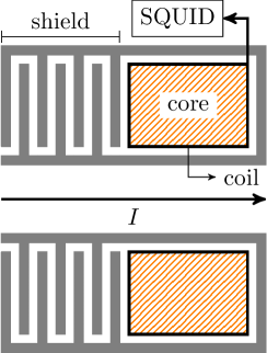
(a) Ring topology.

(b) Folded coaxial topology (opening at the outer radius).

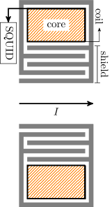
(c) Folded coaxial topology (opening at the inner radius).

Figure 1: Three possible cryogenic current comparators (axial cuts, two dimensional schematics).

The aim of the CCC shield is to reject any external magnetic flux, while remaining transparent to the induction field originated from the electric current to be measured. This property is obtained by choosing an appropriate shield geometry. Furthermore, the specific construction leads to current measurements which are insensitive to the transverse displacement of the line current with respect to the symmetry axis of the CCC. These features are the keystones of the CCC’s exceptional precision, but are only achievable with superconducting materials. Many shield topologies and geometries have been proposed and studied in the literature [4, 5, 6, 7, 8]. In this work, we investigate the performance of a folded coaxial shield (depicted in Figures 1(b) and  1(c)), which is, to the best of our knowledge, studied here for the first time. This shield configuration is compared to the ring structure (depicted in Figure 1(a)) found in several CCCs dedicated to the diagnostics of particle beams in accelerator facilities [9, 10, 11, 12]. In this comparison, the shields geometries are constrained by the radius of the beam tube and the cross-sectional area of the CCC pickup core.

This paper is organized as follows. In section 2, the shielding performance of the coaxial shield is reviewed. Then, in section 3, the new folded coaxial shield is introduced and its performance is analyzed. To this end, an analytical model is first developed, and then validated by means of finite element simulations. The paper continues by reviewing the shielding properties of the ring configuration in section 4. A performance comparison between the ring and folded coaxial topologies is then presented in section 5. Finally, conclusions are drawn in section 6.

2 Coaxial shield

Let us start by reviewing the classical results for the coaxial shield presented in Figures 2 and 3. It can be shown that this shield configuration attenuates every component of the magnetic induction field, with the exception of the azimuthal one [6]. Moreover, the theory reveals that the component undergoing the weakest (but still existing) damping from the shield has the following property: it is spatially constant (in Cartesian coordinates) and perpendicular to the CCC axis, as shown in Figure 4. Thus, it is sufficient to analyze the damping experienced by this component in order to assess the performance of the shield. Let us formally define the global damping profile $d_{\mathcal{C}}(s)$ and the local damping profile $\delta_{\mathcal{C}}(s)$ of the least damped field along a curve $\mathcal{C}$ parameterized by $s\in[s_{\text{min}},s_{\text{max}}]\subset\mathbb{R}$:

$$d_{\mathcal{C}}(s)= \displaystyle\frac{B_{\text{in}}}{B(s)},$$ (1a)

$$\delta_{\mathcal{C}}(s)= \displaystyle\frac{B(s_{\text{min}})}{B(s)},$$ (1b)

where $B$ is the magnitude of the magnetic induction and $B_{\text{in}}$ the magnitude of the magnetic induction at the CCC opening.

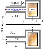
Figure 2: Coaxial configuration of a CCC shield (axial cut, two dimensional schematic); the symbol $\bullet$ indicates the origin of a curve (i.e. the location of its parametric coordinate $s_{\text{min}}$).

Figure 3: Coaxial configuration of a CCC shield (axial cut, three dimensional CAD view, CCC axis depicted as a blue line).

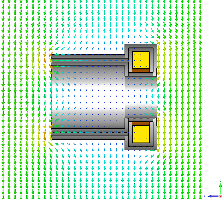
Figure 4: Example of a source magnetic induction field undergoing the weakest damping from the shield (axial cut, arbitrary scale).

The only difference between these two definitions is the normalization procedure: i) in the global case, the damping is normalized with respect to the field intensity at the CCC opening; ii) in the local case, the damping is normalized with respect to the field intensity at the origin of $\mathcal{C}$, which depends on the definition of the curve. Let us note that in the example given in Figure 2, the quantities $d_{\mathcal{C}_{\text{coax}}}(s)$ and $\delta_{\mathcal{C}_{\text{coax}}}(s)$ are identical, since the origin $s_{\text{min}}$ of $\mathcal{C}_{\text{coax}}$ is located at the CCC opening. On the other hand, if we take the example of the curve $\mathcal{C}^{2}_{\text{folded}}$ depicted in Figure 6, the values given by $d_{\mathcal{C}^{2}_{\text{folded}}}(s)$ and $\delta_{\mathcal{C}^{2}_{\text{folded}}}(s)$ will be different, since $s_{\text{min}}$ is not located at the CCC opening. Of course, in order to assess the performance of a shield, the global damping profile is of interest. However, the local variant eases the analysis of complex structures.

With this definition in hand, the global damping profile of the coaxial shield is [6]:

$$d_{\mathcal{C}_{\text{coax}}}(s)=\exp\left(\frac{s}{R_{\text{out}}}\right)\quad\forall s\in[0,L],$$ (2)

where $R_{\text{out}}$ is the outer radius of the coaxial shield, and where the curve $\mathcal{C}_{\text{coax}}$ is a straight segment starting at the CCC opening and traveling along the whole shield of length $L$, as depicted in Figure 2. The coaxial structure thus offers an exponential damping profile. For a particular section $\widetilde{\mathcal{C}}_{\text{coax}}$ of $\mathcal{C}_{\text{coax}}$, the local damping is given by:

$$\delta_{\widetilde{\mathcal{C}}_{\text{coax}}}(s)=\exp\left(\frac{s-s_{\text{min}}}{R_{\text{out}}}\right)\,\,\,\forall s\in[s_{\text{min}},s_{\text{max}}],$$ (3)

where $0\leq s_{\text{min}}\leq s_{\text{max}}\leq L$. Finally, let us mention that the above results have been derived under the following assumptions [6]:

1. the superconducting material is assumed to be ideal and perfectly described by the London equations;

2. the thickness (denoted by $t$ in Figure 2) of the superconducting shield is larger than its London penetration depth, so that perfect diamagnetism can be assumed;

3. the thickness of the superconducting shield, as well as the size of the shield air gap (denoted by $g$ in Figure 2), are small compared to the inner and outer radii of the CCC.

3 Folded coaxial shield

From (2), it is evident that the overall attenuation achieved by the shield depends on its length. Unfortunately, this can lead to a structure with an excessive size in the axial direction. A natural solution to circumvent this limitation is to fold the coaxial structure in the radial direction, as indicated in Figure 5. This leads to a folded coaxial shield forming a meander-like structure, as depicted in Figure 6.

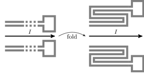
Figure 5: Folding a coaxial shield into a meander structure (axial cut).

3.1 Two possible variants for the folded coaxial CCC

After folding of the coaxial shield structure, two possibilities remain for completing the CCC: the detection coil is either located at the inner, or at the outer radius of the shield, as shown in Figure 6. Evidently, the opening of the folded coaxial shield is located at the opposite radius. In the following, the inner variant refers to the CCC with the meander opening at the inner radius, and the outer variant refers to the other case. As discussed later in this paper, both variants show different behavior.

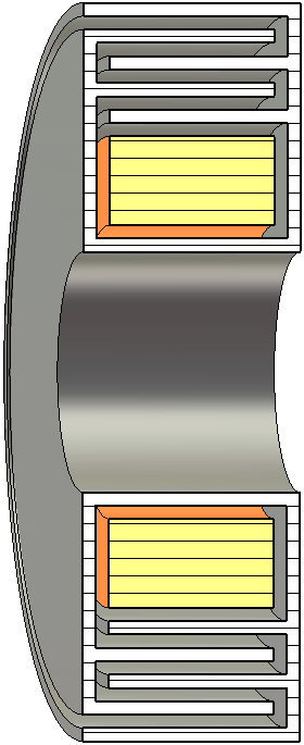
(a) Three dimensional CAD view of the outer variant (opening at the outer radius).

(b) Two dimensional schematic of the outer variant (opening at the outer radius).

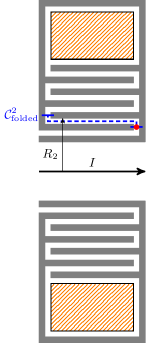
(c) Two dimensional schematic of the inner variant (opening at the inner radius).

Figure 6: The two possible variants for the folded coaxial CCC (axial cuts); the symbol $\bullet$ indicates the origin of a curve (i.e. the location of its parametric coordinate $s_{\text{min}}$).

3.2 Analytical damping profile

Analyzing the shape of a folded coaxial shield, we can directly notice that the structure is a set of coaxial cylinders concentrically stacked around each others. Therefore, for one shell of the stack, the local damping defined in (3) holds, if an appropriate redefinition of the curve $\mathcal{C}$ and its corresponding outer radius $R_{\text{out}}$ is given.

Let us start by considering a folded coaxial shield consisting of a stack of $N$ shells, each shell being identified by an index $i\in\{1,\dots,N\}$. For the $i$^th shell, the curve $\mathcal{C}_{\text{folded}}^{i}$ is composed of the $i$^th straight section and half of the $(i-1)$^th and $(i+1)$^th linking parts, as depicted in Figure 6. We then introduce a parameter $s\in[\ell_{i-1},\ell_{i}]$ to parametrize $\mathcal{C}_{\text{folded}}^{i}$, where $\ell_{i}$ is the total unfolded length between the CCC opening and the end of $\mathcal{C}_{\text{folded}}^{i}$. By convention, we further impose that $\ell_{0}=0$. With these definitions, and by exploiting (3), the local damping introduced by the $i$^th shell writes:

$$\delta_{\mathcal{C}_{\text{folded}}^{i}}=\exp{\left(\frac{s-\ell_{i-1}}{R_{i}}\right)}\quad\forall s\in[\ell_{i-1},\ell_{i}],$$ (4)

where $R_{i}$ is the outer radius of the $i$^th shell. It is worth mentioning that this equation does not consider the variation of $R_{i}$ along the linking parts constituting $\mathcal{C}_{\text{folded}}^{i}$. However, thanks to the 0 hypothesis (see section 2), this simplification is legitimate.

The global damping $d_{\mathcal{C}_{\text{folded}}^{i}}$ introduced by the $i$^th shell is computed as follows. By combining (1b) and (1a), we have:

$$d_{\mathcal{C}}(s)=\frac{B_{\text{in}}}{B(s_{\text{min}})}\delta_{\mathcal{C}}(s)\quad\forall s\in[s_{\text{min}},s_{\text{max}}].$$ (5)

Thus, by inserting (4) in (5), we can write:

$$d_{\mathcal{C}_{\text{folded}}^{i}}(s)=\alpha_{i}\delta_{\mathcal{C}_{\text{folded}}^{i}}(s)\quad\forall s\in[\ell_{i-1},\ell_{i}],$$ (6)

where, by exploiting (1a) (the definition of $d_{\mathcal{C}}$), the coefficient $\alpha_{i}$ is given by

$$\alpha_{i}=\frac{B_{\text{in}}}{B(s_{\text{min}})}=d_{\mathcal{C}_{\text{folded}}^{i}}(\ell_{i-1}).$$ (7)

Physically speaking, this coefficient $\alpha_{i}$ accounts for the damping introduced by the $(i-1)$ previous shells.

Let us now show that the following holds:

$$\alpha_{1}=1\quad\text{and}\quad\alpha_{i+1}=\alpha_{i}\exp{\left(\frac{\ell_{i}-\ell_{i-1}}{R_{i}}\right)}.$$ (8)

Since for the first shell we have $B(s_{\text{min}})=B_{\text{in}}$ by definition of $\mathcal{C}_{\text{folded}}^{1}$, we can directly exploit (7) to show that $\alpha_{1}=1$. Furthermore, by combining the definitions (6), (7) and the local damping (4), we can write:

$$d_{\mathcal{C}_{\text{folded}}^{i}}(s)=d_{\mathcal{C}_{\text{folded}}^{i}}(\ell_{i-1})\exp{\left(\frac{s-\ell_{i-1}}{R_{i}}\right)}$$

$$\forall s\in[\ell_{i-1},\ell_{i}].$$ (9)

Moreover, because of the continuity of the magnetic induction, we have that:

$$d_{\mathcal{C}_{\text{folded}}^{i+1}}(\ell_{i})=d_{\mathcal{C}_{\text{folded}}^{i}}(\ell_{i}).$$ (10)

Thus, by evaluating (9) at $s=\ell_{i}$ and by using (10), the following holds:

$$d_{\mathcal{C}_{\text{folded}}^{i}}(\ell_{i}) =d_{\mathcal{C}_{\text{folded}}^{i+1}}(\ell_{i}),$$

$$=d_{\mathcal{C}_{\text{folded}}^{i}}(\ell_{i-1})\exp{\left(\frac{\ell_{i}-\ell_{i-1}}{R_{i}}\right)}.$$ (11)

Then, by exploiting once more the definition (7), we can conclude the proof:

$$\alpha_{i+1}=\alpha_{i}\exp{\left(\frac{\ell_{i}-\ell_{i-1}}{R_{i}}\right)}.$$ (12)

From these last results, it worth noticing that, the total damping exhibited by the shield

$$d_{\mathcal{C}_{\text{folded}}^{N}}(\ell_{N}) =\alpha_{N}\delta_{\mathcal{C}_{\text{folded}}^{N}}(\ell_{N}),$$

$$=\alpha_{N-1}\exp\left(\frac{\ell_{N-1}-\ell_{N-2}}{R_{N-1}}\right)$$

$$\exp\left(\frac{\ell_{N}-\ell_{N-1}}{R_{N}}\right),$$

$$=\dots,$$

$$=\alpha_{N-(N-1)}$$

$$\phantom{=}~{}\exp\left(\frac{\ell_{N-(N-1)}-\ell_{N-(N-1)-1}}{R_{N-(N-1)}}\right)\dots$$

$$\exp\left(\frac{\ell_{N}-\ell_{N-1}}{R_{N}}\right),$$

$$=\prod_{i=1}^{N}\exp\left(\frac{\ell_{i}-\ell_{i-1}}{R_{i}}\right),$$ (13)

appears naturally as the product of the damping introduced by each layer.

3.3 Numerical validation

To validate the analytical damping model (6) and (8), we arranged a numerical finite element (FE) simulation, utilizing the magnetostatic solver provided in CST EM STUDIO^©[13]. The superconducting parts of the CCC are considered as perfect electrical conductors, the relative magnetic permeability of the pickup core is set to $\mu_{r}^{\text{core}}=1000$ and the dimensions of the CCC are given in Table 1. The simulation model embeds the CCC in a spatially constant magnetic field perpendicular to the CCC axis, as the one depicted in Figure 4. The computed magnetic induction field is then sampled along a path following the meanders of the structure. By normalizing the magnitude of the magnetic induction, the damping introduced by the folded coaxial structure was assessed. The numerical results were validated by comparing simulations with different mesh curvatures and FE discretization orders. In the following, the computed dampings are expressed in decibel (dB), following the convention:

$$d^{\text{dB}}_{\mathcal{C}}(s)=20\log_{10}{\Big{(}d_{\mathcal{C}}(s)\Big{)}}.$$ (14)

Gap	Thickness	Inner radius
$0.5$mm	$3$mm	$120$mm
Axial length	Core height	Shells
$120$mm	$50$mm	$24$

Table 1: Main geometrical parameters for the FE simulations.

The finite element results, as well as the predictions given by the analytical model (6) and (8), are summarized in Figure 7 for the inner and outer variants. First, it can directly be noticed that the numerical solutions and the analytical model match well, which comforts us in the validity of our previous developments and assumptions. Maximum relative deviations of $10\%$ and $5\%$ are observed for the outer and inner variants respectively. Secondly, the variant with the meander opening at the inner radius exhibits a larger final damping than the other variant. This phenomenon is easily explained by the fact that the two variants are not symmetric. Indeed, because of the detection coil, the radii of the coaxial shells forming the shield do not span the same range: $R_{i}^{\text{inner}}\in[120,201]$mm for the inner variant and $R_{i}^{\text{outer}}\in[254,173]$mm for the outer one. Furthermore, and as explained in the previous subsection, the local damping introduced by the $i$^th coaxial shell is given by (4) and is proportional to $\exp(1/R_{i})$. Therefore, since the values taken by the sequence $R^{\text{inner}}_{i}$ are smaller or equal to the values taken by the sequence $R^{\text{outer}}_{i}$, the inner variant must exhibit a larger final damping. Finally, we can observe that the damping profile of the inner variant shows a decreasing derivative, while the outer alternative shows an increasing one. This behavior is again easily explained. For the inner variant, as we enter deeper in the meander structure, the damping decreases since the radius increases. For the outer variant, the damping increases since the radius decreases.

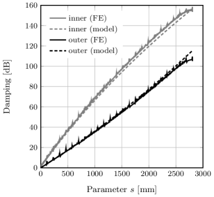
Figure 7: Comparison between FE simulations and equations (6) and (8).

To conclude our numerical validation, we analyzed the influence of the air gap size and of the superconducting material thickness on the damping in more detail. Let us recall that one of our major assumption is that these sizes are small compared to the CCC inner and outer radii. Both parameters are swept over the range $[0.5,2.5]$mm, while keeping the other parameters constant. Before analyzing the results, it is important to stress the following fact: even if the air gap or the thickness do not appear explicitly as a parameter in our model (6) and (8), they impact the considered sequence of radii $R_{i}$. Thus, as the superconductor thickness or the air gap changes, the solution given by (6) and (8) will also change.

The computed results of the damping behavior with respect to the air gap size and the material thickness are shown in Figures 8, 9, 10 and 11. Notice, an increase of the air gap size corresponds to a decrease of the shielding performance, both for the inner and outer variants. Concerning the thickness of the superconducting material, the same behavior as for the air gap size can be observed. Finally, it worth noticing that for each simulation presented in Figures 8, 9, 10 and 11, the maximum relative deviation between the analytical model and the FE simulation did not exceed $10\%$.

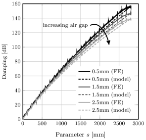
Figure 8: Influence of the air gap (inner variant).

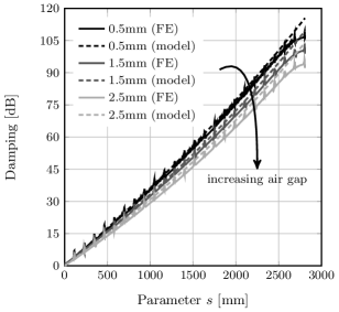
Figure 9: Influence of the air gap (outer variant).

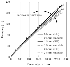
Figure 10: Influence of the thickness of the superconducting material (inner variant).

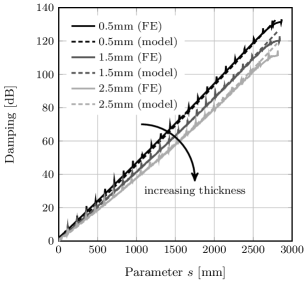
Figure 11: Influence of the thickness of the superconducting material (outer variant).

4 Review of the ring shield

Ring shield CCCs are commonly applied in diagnostic devices of particle beams in accelerator facilities [9, 10, 11, 12]. This shielding configuration exhibits an interleaved comb-like meander structure along the axial direction, as depicted in Figures 12 and 13. This geometry is constructed by successively stacking superconducting rings with different inner and outer radii [14] (hence the name of ring shield). The ring stack gives rise to two families of cavities, as suggested by Figure 12: cavities with increasing and decreasing radius.

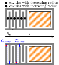
Figure 12: Ring shield configuration (axial cut, two dimensional schematic); the symbol $\bullet$ indicates the origin of a curve (i.e. the location of its parametric coordinate $s_{\text{min}}$).

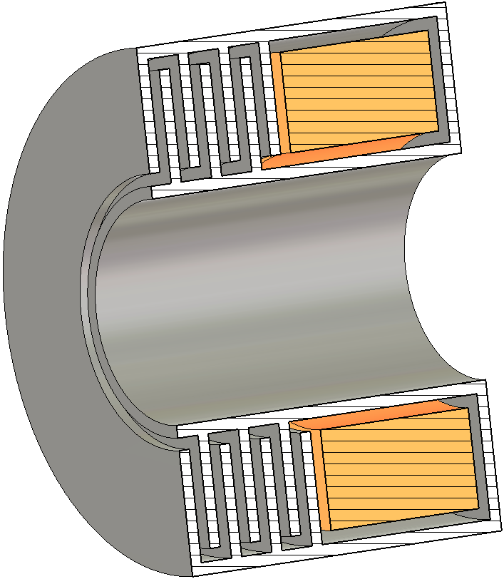
Figure 13: Ring shield configuration (axial cut, three dimensional CAD view).

The local attenuation of cavities with alternating, increasing or decreasing, radius writes, for all $s~{}\in~{}[\ell_{i-1},~{}\ell_{i}]$, as follows [7]:

$$\delta_{\mathcal{C}^{i}_{\text{cavity}}}(s) =\displaystyle\left(\frac{s-\ell_{i-1}}{R_{\text{in}}}+1\right)^{2} \forall i~{}\text{odd}$$ (15a)

$$\delta_{\mathcal{C}^{i}_{\text{cavity}}}(s) =1 \forall i~{}\text{even},$$ (15b)

where the curves upon which these local dampings are defined are depicted in Figure 12, and $\ell_{i}$ is defined in the same way as in the folded coaxial case and $R_{\text{in}}$ is the inner radius of the CCC. Further details can be found in [7]. From Equation (15), it can be directly noticed that only the cavities with an increasing radius are contributing to the local damping, the only goal of a decreasing radius cavity being to connect two increasing cavities. While this behavior can be formally derived from the London-Ampère equations [7], a geometrically driven approach can be found in [14]. Finally, the global damping profile is derived following the same strategy as in the previous section, leading to:

$$d_{\mathcal{C}^{i}_{\text{cavity}}}(s) =\alpha_{i}\left(\frac{s-\ell_{i-1}}{R_{\text{in}}}+1\right)^{2} \forall i~{}\text{odd},$$ (16a)

$$d_{\mathcal{C}^{i}_{\text{cavity}}}(s) =\alpha_{i} \forall i~{}\text{even},$$ (16b)

for all $s\in[\ell_{i-1},\ell_{i}]$, with $\alpha_{1}=1$ and

$$\alpha_{i+1}=\alpha_{i}\times\left\{\begin{array}[]{l@{~}r}\displaystyle\left(\frac{\ell_{i}-\ell_{i-1}}{R_{\text{in}}}+1\right)^{2}\hfil~{}&\,\,\,\forall i~{}\text{odd},\\ 1\hfil~{}&\,\,\,\forall i~{}\text{even}.\end{array}\right.$$ (17)

This last relation is proved by exploiting (7), and by definition of $\mathcal{C}^{1}_{\text{cavity}}$, the equality $\alpha_{1}=1$ comes directly, since $B_{\text{in}}$ equals $B(s_{\text{min}})$ on this curve. Furthermore, by combining the definitions (16) and (7), we can write:

$$d_{\mathcal{C}_{\text{cavity}}^{i}}(s) =d_{\mathcal{C}_{\text{cavity}}^{i}}(\ell_{i-1})\times\left\{\begin{array}[]{l@{~}r}\displaystyle\left(\frac{s-\ell_{i-1}}{R_{\text{in}}}+1\right)^{2},\hfil~{}\\ 1.\hfil~{}\end{array}\right.$$ (20)

We can then evaluate (20) at $s=\ell_{i}$, and by exploiting the continuity condition (10) we get:

$$d_{\mathcal{C}_{\text{cavity}}^{i}}(\ell_{i}) =d_{\mathcal{C}_{\text{cavity}}^{i+1}}(\ell_{i}),$$

$$=d_{\mathcal{C}_{\text{cavity}}^{i}}(\ell_{i-1})\times\left\{\begin{array}[]{l@{~}r}\displaystyle\left(\frac{\ell_{i}-\ell_{i-1}}{R_{\text{in}}}+1\right)^{2},\hfil~{}\\ 1.\hfil~{}\end{array}\right.$$ (23)

Then, by combining (7) and (4), we can conclude the proof:

$$\alpha_{i+1}=\alpha_{i}\times\left\{\begin{array}[]{l@{~}r}\displaystyle\left(\frac{\ell_{i}-\ell_{i-1}}{R_{\text{in}}}+1\right)^{2}\hfil~{}&\,\,\,\forall i~{}\text{odd},\\ 1\hfil~{}&\,\,\,\forall i~{}\text{even}.\end{array}\right.$$ (24)

From these last results, it worth noticing that the total damping exhibited by a shield composed of $2N$ rings writes:

$$\begin{array}[]{ll}&d_{\mathcal{C}_{\text{cavity}}^{2N}}(\ell_{2N})\\ =&\alpha_{2N}\times\delta_{\mathcal{C}_{\text{cavity}}^{2N}}(\ell_{2N}),\\ =&\alpha_{2N}\times 1,\\ =&\alpha_{2N-1}\times\left(\frac{\ell_{2N-1}-\ell_{2N-2}}{R_{\text{in}}}+1\right)^{2},\\ =&\alpha_{2N-2}\times 1\times\left(\frac{\ell_{2N-1}-\ell_{2N-2}}{R_{\text{in}}}+1\right)^{2},\\ =&\alpha_{2N-3}\times\left(\frac{\ell_{2N-3}-\ell_{2N-4}}{R_{\text{in}}}+1\right)^{2}\\ &\phantom{\alpha_{2N-3}}\times\left(\frac{\ell_{2N-1}-\ell_{2N-2}}{R_{\text{in}}}+1\right)^{2},\\ =&\dots,\\ =&\alpha_{2N-(2N-1)}\times\left(\frac{\ell_{2N-(2N-1)}-\ell_{2N-(2N-1)-1}}{R_{\text{in}}}+1\right)^{2}\\ &\phantom{\alpha_{2N-(2N-1)}}\times\dots\\ &\phantom{\alpha_{2N-(2N-1)}}\times\left(\frac{\ell_{2N-3}-\ell_{2N-4}}{R_{\text{in}}}+1\right)^{2},\end{array}$$

which leads to

$$d_{\mathcal{C}_{\text{cavity}}^{2N}}(\ell_{2N})=\prod_{i=1}^{N}\left(\frac{\ell_{2i-1}-\ell_{2i-2}}{R_{\text{in}}}+1\right)^{2},$$ (25)

and is, as expected, nothing but the product of the damping introduced by each pair of increasing-decreasing rings.

5 Volumetric performance comparison

By comparing the damping profiles of a ring (15) and a folded coaxial shield (4), the main differences between the two topologies appear clearly, and are summarized in Table 2. The first motivation to choose one topology over the other is related to space constraints. Depending on the available space, one may be interested in building a CCC expanding in the radial or the axial direction. On the other hand, if space is not a constraint, one is interested in building the lightest shield for a given total damping, i.e. a shield exhibiting the smallest volume. In this case, the exponential damping profile of the folded coaxial shield seems the most attractive. However, the situation is unfortunately not that simple.

Parameter	Folded coaxial	Ring
Damping profile	Exponential	Quadratic (increasing ring)
of a layer		No damping (decreasing ring)
Efficiency of each	Decreases (inner variant)	Constant
additional layer	Increases (outer variant)
Stacking direction	Radial	Axial

Table 2: Comparison between folded coaxial and ring shields.

5.1 Single layer case

Let us consider a single increasing radius cavity and a coaxial shell. The local dampings are given by (15) and (4) respectively. Furthermore, we have that $i=1$, $\ell_{i-1}=0$ and $R_{i}=R_{\text{in}}+g\approx R_{\text{in}}$, since we assumed the air gap $g$ to be negligible with respect to $R_{\text{in}}$. In this case, we have:

$$\Delta(s) =\delta_{\mathcal{C}_{\text{cavity}}^{1}}(s)-\delta_{\mathcal{C}_{\text{folded}}^{1}}(s),$$

$$=\left(\frac{s}{R_{\text{in}}}+1\right)^{2}-\exp\left(\frac{s}{R_{\text{in}}}\right).$$ (26)

The real-valued roots of the function $\Delta(s)$ are found using the symbolic solver of Wolfram Mathematica [15], and are given by:

$$\begin{array}[]{r@{~}l}\displaystyle\frac{s}{R_{\text{in}}}\in\Bigg{\{}~{}&\overbrace{-1-2W_{0}\left(\frac{1}{2\sqrt{e}}\right)}^{\approx-1.5},\\ ~{}&0,\\ ~{}&\underbrace{-1-2W_{-1}\left(-\frac{1}{2\sqrt{e}}\right)}_{\approx+2.5}\Bigg{\}},\end{array}$$

where $W_{0}$ and $W_{-1}$ are the two real branches of the Lambert $W$ function [16]. Furthermore, by analyzing the graph of $\Delta(s)$, depicted in Figure 14, it is clear that this function is:

• positive for $s\in]-\infty,-1.5R_{\text{in}}[$ and
  $s\in]0,2.5R_{\text{in}}[$;

• negative for $s\in]-1.5R_{\text{in}},0[$ and
  $s~{}\in~{}]2.5R_{\text{in}},+\infty[$.

These results leads us then to the following conclusion: let an increasing radius ring and a coaxial shell of the same size $\tilde{\ell}$ be given, then the following holds

$$\delta_{\mathcal{C}_{\text{folded}}^{1}}(\tilde{\ell})\geq\delta_{\mathcal{C}_{\text{cavity}}^{1}}(\tilde{\ell})\quad\text{if}\quad\tilde{\ell}\geq 2.5R_{\text{in}}.$$ (27)

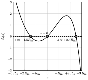
Figure 14: Graph of $\Delta(s)$.

Therefore, despite its exponential damping, the folded coaxial CCC will not necessarily exhibit a better damping than its ring alternative, at least for the first ring or coaxial shell.

5.2 General case

For a more realistic analysis of volume and shielding performances, the following numerical experiment is carried out: for the three CCC shields presented above (ring, inner folded coaxial and outer folded coaxial) we compute the damping corresponding to different axial lengths $L$, outer radius sizes $R_{\text{out}}$ and numbers of meanders. Among all these configurations, the inner radius $R_{\text{in}}$ and the core cross section $S_{\text{core}}$ are held constant, as reported in Table 3. Then, for each result, the shield volume is approximated by using the equations given in Table 4.

Constrained parameter	Constraint value
Inner radius ($R_{\text{in}}$)	$120$mm
Core cross section ($S_{\text{core}}$)	$60$cm2

Table 3: Constraints for the performance comparison.

		Folded coaxial shield CCC
Volume	Ring shield CCC	Inner variant	Outer variant
Total ($V_{T}$)	$\pi\,R_{\text{out}}^{2}\,L$	$\pi\,R_{\text{out}}^{2}\,L$	$\pi\,R_{\text{out}}^{2}\,L$
Interior($V_{I}$)	$\pi\,R_{\text{in}}^{2}\,L$	$\pi\,R_{\text{in}}^{2}\,L$	$\pi\,R_{\text{in}}^{2}\,L$
Core ($V_{C}$)	$\pi\,(R_{\text{out}}^{2}-R_{\text{in}}^{2})\,L_{C}$	$V_{T}-\pi\,(R_{\text{out}}-H_{C})^{2}\,L$	$\pi\,(R_{\text{in}}+H_{C})^{2}\,L-V_{I}$
Shield ($V_{S}$)	$\pi\,(R_{\text{out}}^{2}-R_{\text{in}}^{2})\,L_{S}$	$V_{T}-V_{I}-V_{C}$	$V_{T}-V_{I}-V_{C}$
Length
Core ($L_{C}$)	$S_{\text{core}}/H_{C}$	$L$	$L$
Shield ($L_{S}$)	$L-L_{C}$	$L$	$L$
Height
Core ($H_{C}$)	$R_{\text{out}}-R_{\text{in}}$	$S_{\text{core}}/L$	$S_{\text{core}}/L$

Table 4: Volumes definitions.

The computed results are depicted in Figure 15. The plots are organized as follows. Each computed configuration is depicted as a colored dot in the axial length – outer radius plane. The color of this dot corresponds to the damping exhibited by the considered shield. Among all these possibilities, some are sharing the same number of meanders, and are thus connected by dashed lines, further called iso-meander lines. Moreover, since the shield volume is only a function of the axial length and the outer radius (for a fixed core cross section and inner radius), it makes sens to additionally represent the iso-shield-volume lines on the plots.

With all these information in hand, the optimization process becomes rather easy. Since we can directly access the axial length and the outer radius, we can easily reject or accept a configuration with respect to space constraints. In our experiment, we restricted ourselves to the arbitrary range: $L\in[90,210]$mm and $R_{\text{out}}\in[165,250]$mm. Once this admissible range defined, we can select the configurations sharing the same damping. Thanks to the iso-meander lines, we can directly retrieve the corresponding number of meanders. It is worth stressing that in the ring topology, the axial length depends on the number of meanders and the outer radius is a free parameter, while the situation is reverted for the folded coaxial cases. In our numerical setup, we chose to consider dampings in the range $75$dB $\pm 5$dB. Then, we can search on which iso-shield-volume lines the selected candidates are lying. Finally, the configuration leading to the minimal shield volume can be selected, as shown in Table 5.

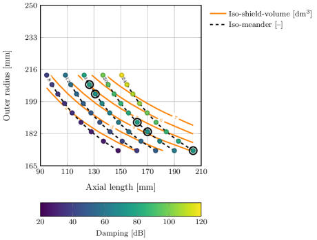
(a) Ring shield.

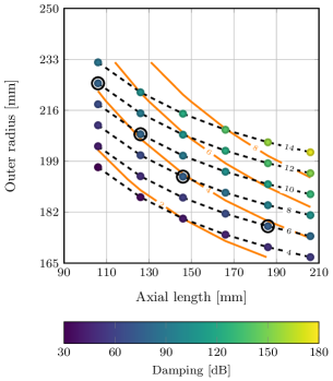
(b) Folded coaxial shield (inner variant).

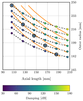
(c) Folded coaxial shield (outer variant).

Figure 15: Shield volumetric performance for different configurations, where the encircled configurations exhibit a damping in the range $75$dB $\pm 5$dB and the fixed parameters are set to $R_{\text{in}}=120$mm and $S_{\text{core}}=60$cm².

	Volume
Type	Shield	Core	Damping	Outer radius	Axial length	Shell/Ring
Ring	$4.1$dm3	$5.9$dm3	$76$dB	$173$mm	$204$mm	$24$
Inner	$3.7$dm3	$6.3$dm3	$74$dB	$177$mm	$186$mm	0$6$
Outer	$6.1$dm3	$5.3$dm3	$75$dB	$184$mm	$186$mm	0$8$

Table 5: Shields with minimal volumes, where inner and outer designate the inner and outer variants of the folded coaxial shield (fixed parameters $R_{\text{in}}=120$mm and $S_{\text{core}}=60$cm²).

By analyzing the damping and volume characteristics reflected in Figure 15, the following conclusion can be drawn. In the case of the ring configuration, the shield volume is minimized by favoring small outer radii and a large number of meanders. On the other hand, in the case of the folded coaxial topology, the shield volume is minimized when a small amount of long meanders is used. This behavior is easily explained, since the shield volume depends quadratically on the shield outer radius and linearly on the shield length. Therefore, a reduction of the outer radius is more effective in the ring configuration, even if this reduction calls for an increase in the number of meander, and thus an increase in the shield length. The same reasoning can be applied for the folded coaxial case: a decrease of the outer radii calls for a reduction in the number of meanders, which must be compensated by increasing the length of one meander.

Furthermore, by exploiting the data presented in Table 5, it becomes clear that among the different shield topologies, the inner variant of the folded coaxial approach leads to the lightest (i.e. with the smallest volume) shield. However, the weight of the total CCC is also determined by its magnetic core. If we now analyze its occupied volume, the outer counterpart becomes more interesting. It is then worth mentioning that if the densities of the materials used are known, the presented optimization can be improved: instead of using iso-shield-volume (or iso-core-volume) lines, it is more interesting to directly use iso-mass lines, computed by weighting the core and shield volumes by their respective densities.

6 Conclusion

In this paper, we analyzed the performance of a folded superconducting coaxial shield for a cryogenic current comparator. The damping profile presented by this new shield topology was first estimated with an analytical model, which was then validated by means of finite element simulations. In all the carried out simulations, the relative difference between the two approaches did not exceed $10\%$.

By analyzing the newly proposed analytical model, we realized that the damping efficiency of each additional coaxial layer was not constant, as in the ring topology. Indeed, depending on whether the CCC opening is located at the inner or outer radius, the damping efficiency of an additional shielding layer decreases or increases, respectively. Furthermore, because of the space taken by the detection coil, the radii of the coaxial shells cannot span the same range. Therefore, the overall performance of the inner and outer variants cannot be identical.

Finally, this work compared the ring topology with the two variants of the folded coaxial shield. At this point, different shield configurations were tested, in which the inner radius and the core cross section have been held constant (in particular, these parameters were fixed to $120$mm and $60$cm²). Among all the considered configuration, only those leading to a total damping in the range $75$dB $\pm 5$dB were selected. This numerical experiment led us to the following conclusions: i) in the case of a ring topology, the shield volume is minimized by favoring small outer radii and a large number of meanders; ii) in the case of a folded coaxial topology, the shield volume is minimized by favoring a small amount of long meanders.

References

- [1] I. K. Harvey, A precise low temperature dc ratio transformer, Review of Scientific Instruments 43 (11) (1972) 1626–1629. doi:10.1063/1.1685508.
- [2] J. M. Williams, Cryogenic current comparators and their application to electrical metrology, IET Science, Measurement and Technology 5 (6) (2011) 211–224. doi:10.1049/iet-smt.2010.0170.
- [3] J. Clarke, A. I. Braginski (Eds.), The SQUID Handbook: Fundamentals and Technology of SQUIDs and SQUID Systems, Wiley-VCH, Weinheim, 2004. doi:10.1002/3527603646.
- [4] D. B. Sullivan, R. F. Dziuba, Low temperature direct current comparators, Review of Scientific Instruments 45 (4) (1974) 517–519. doi:10.1063/1.1686674.
- [5] K. Grohmann, H. D. Hahlbohm, H. Lübbig, H. Ramin, Ironless cryogenic current comparators for AC and DC applications, IEEE Transactions on Instrumentation and Measurement 23 (4) (1974) 261–263. doi:10.1109/TIM.1974.4314287.
- [6] K. Grohmann, H. D. Hahlbohm, D. Hechtfischer, H. Lübbig, Field attenuation as the underlying principle of cryo current comparators, Cryogenics 16 (7) (1976) 423–429. doi:10.1016/0011-2275(76)90056-4.
- [7] K. Grohmann, H. D. Hahlbohm, D. Hechtfischer, H. Lübbig, Field attenuation as the underlying principle of cryo-current comparators 2. Ring cavity elements, Cryogenics 16 (10) (1976) 601–605. doi:10.1016/0011-2275(76)90192-2.
- [8] H. Seppa, The ratio error of the overlapped-tube cryogenic current comparator, IEEE Transactions on Instrumentation and Measurement 39 (5) (1990) 689–697. doi:10.1109/19.58609.
- [9] A. Peters, W. Vodel, H. Koch, R. Neubert, H. Reeg, C. H. Schroeder, A cryogenic current comparator for the absolute measurement of nA beams, AIP Conference Proceedings 451 (1) (1998) 163–180. doi:10.1063/1.56997.
- [10] T. Tanabe, K. Chida, K. Shinada, A cryogenic current-measuring device with nano-ampere resolution at the storage ring TARN II, Nuclear Instruments and Methods in Physics Research Section A: Accelerators, Spectrometers, Detectors and Associated Equipment 427 (3) (1999) 455–464. doi:10.1016/S0168-9002(99)00058-3.
- [11] R. Geithner, W. Vodel, R. Neubert, P. Seidel, F. Kurian, H. Reeg, M. Schwickert, An improved cryogenic current comparator for FAIR, in: 3rd International Particle Accelerator Conference IPAC’12, 2012, pp. 822–824.
- [12] M. Fernandes, R. Geithner, J. Golm, R. Neubert, M. Schwickert, T. Stöhlker, J. Tan, C. P. Welsch, Non-perturbative measurement of low-intensity charged particle beams, Superconductor Science and Technology 30 (1) (2017) 015001. doi:10.1088/0953-2048/30/1/015001.
- [13] Computer Simulation Technology AG, CST EM STUDIO©, www.cst.com (2015).
- [14] H. De Gersem, N. Marsic, W. F. O. Müller, F. Kurian, T. Sieber, M. Schwickert, Finite-element simulation of the performance of a superconducting meander structure shielding for a cryogenic current comparator, Nuclear Instruments and Methods in Physics Research Section A: Accelerators, Spectrometers, Detectors and Associated Equipment 840 (2016) 77–86. doi:10.1016/j.nima.2016.10.003.
- [15] Wolfram Research, Inc., Mathematica, Version 11.0, Champaign, IL (2016).
- [16] R. M. Corless, G. H. Gonnet, D. E. G. Hare, D. J. Jeffrey, D. E. Knuth, On the Lambert W function, Advances in Computational Mathematics 5 (1) (1996) 329–359. doi:10.1007/BF02124750.