Computational Optics Meet Domain Adaptation: Transferring Semantic Segmentation Beyond Aberrations

Abstract

Semantic scene understanding with Minimalist Optical Systems (MOS) in mobile and wearable applications remains a challenge due to the corrupted imaging quality induced by optical aberrations. However, previous works only focus on improving the subjective imaging quality through computational optics, i.e. Computational Imaging (CI) technique, ignoring the feasibility in semantic segmentation. In this paper, we pioneer to investigate Semantic Segmentation under Optical Aberrations (SSOA) of MOS. To benchmark SSOA, we construct Virtual Prototype Lens (VPL) groups through optical simulation, generating Cityscapes-ab and KITTI-360-ab datasets under different behaviors and levels of aberrations. We look into SSOA via an unsupervised domain adaptation perspective to address the scarcity of labeled aberration data in real-world scenarios. Further, we propose Computational Imaging Assisted Domain Adaptation (CIADA) to leverage prior knowledge of CI for robust performance in SSOA. Based on our benchmark, we conduct experiments on the robustness of state-of-the-art segmenters against aberrations. In addition, extensive evaluations of possible solutions to SSOA reveal that CIADA achieves superior performance under all aberration distributions, paving the way for the applications of MOS in semantic scene understanding.

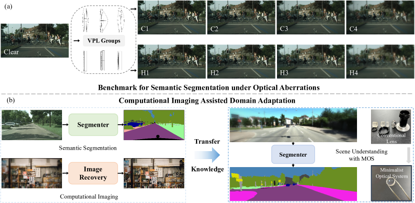
Figure 1: (a) A comprehensive benchmark for Semantic Segmentation under Optical Aberrations (SSOA). We construct Virtual Prototype Lens (VPL) groups with different behaviors and levels of aberrations to map clear image into simulated imaging results. (b) Proposed Computational Imaging Assisted Domain Adaptation (CIADA) for SSOA with the prior knowledge of computational imaging. We pioneer scene understanding with Minimalist Optical System (MOS). i.e. transferring semantic segmentation beyond aberrations. Compared to conventional lens, MOS has a simple structure, which is beneficial for a wide variety of applications in mobile and wearable devices.

1 Introduction

Semantic scene understanding attracts considerable research interests for its potential applications in autonomous driving [56, 75], augmented reality [50], and robot navigation [18]. As the demand for thin, portable imaging systems grows stronger in mobile and wearable applications, semantic perception with Minimalist Optical Systems (MOS) [24, 42], which can image over a large Field of View (FoV) with only a few optical elements (shown at the lower right corner of Fig. 1), has come to the research forefront.

However, Semantic Segmentation under Optical Aberrations (SSOA) has been barely investigated. One major challenge lies in the scarcity of labeled training data, corrupted by aberrations, for yielding robust segmentation models [9, 41]. Yet, it is cost-intensive to acquire large-scale pixel-wise labeled data, in particular for aberration images which are harder to annotate. While imaging simulation can generate target images from existing datasets, the synthetic-to-real gap remains a potential problem. Meanwhile, the recent progress in Unsupervised Domain Adaptation (UDA) has brought promising solutions [22, 47, 88], which offers a novel perspective to supplement the coverage of training data in unseen scenarios. In this paper, we look at SSOA through the lens of UDA by distilling knowledge from label-rich clean data to label-scarce aberration data.

To this intent, we formalize the task of UDA for SSOA in a comprehensive benchmark through wave-based imaging simulation [49]. We summarize aberration behaviors of MOS: Common Simple Lens (CSL, i.e. spatial-variant degradation) and Hybrid Refractive Diffractive Lens (HRDL, i.e. spatial-uniform degradation), and construct Virtual Prototype Lens (VPL) groups to produce simulated imaging results of different MOS. VPL groups contain randomly generated aberration distributions of four levels for CSL and HRDL, respectively (see Fig. 1(a)). Specifically, we create Cityscapes-ab and KITTI-360-ab to benchmark semantic segmentation under various optical aberrations.

Computational optics for imaging systems, i.e. Computational Imaging (CI), appear as a preferred solution to the optimization of MOS. The degraded images induced by optical aberrations are recovered through learning-based image restoration models [11, 55] for comparable imaging results to conventional lens. However, contemporary CI techniques are isolated from the potential applications of MOS in semantic perception. Previous methods only produce recovered images optimized for human observation, ignoring the corrupted data distribution for segmenters [52], which leads to even worse performance [65]. The extra computation overhead of recovery also hinders their implementations in real applications.

To this end, we propose a Computational Imaging Assisted Domain Adaptation (CIADA) framework for domain adaptive SSOA. As shown in Fig. 1 (b), the knowledge of semantic segmentation on clear image and CI is transferred to the target domain for SSOA, without any additional computational overhead during inference. We put forward a Bidirectional Teacher solution to store the image degradation knowledge from CI through image degradation and recovery. Further, an auxiliary decoder for image recovery with correlation-based distillation is designed to distill the CI knowledge to the target segmenter.

Based on the benchmark, we conduct comprehensive evaluations on the influence of aberrations on state-of-the-art segmenters, revealing that aberrations bring considerable damages to the segmentation performance. Additionally, extensive experiments on possible solutions to SSOA show that CIADA outperforms the state-of-the-art UDA method [22] by $3.29/4.02$ in mIoU on Cityscapes [9]${\to}$KITTI-360-ab and $2.28/3.48$ in mIoU on KITTI-360 [41]${\to}$Cityscapes-ab. CIADA is a successful attempt to combine advanced CI techniques with unsupervised domain adaptive SSOA, paving the way for MOS-driven scene understanding.

In summary, it is the first work to address semantic segmentation under severe optical aberrations of MOS to the best of our knowledge. We deliver four main contributions:

• We explore the applications of minimalist optical systems in semantic scene understanding, i.e., semantic segmentation beyond optical aberrations, from an unsupervised domain adaptation perspective.

• We benchmark the task through Virtual Prototype Lens (VPL) groups, which can translate existing datasets into corrupted images under various levels of aberrations. We provide Cityscapses-ab and KITTI-360-ab to foster semantic perception under aberrations.

• We propose Computational Imaging Assisted Domain Adaptation, coined CIADA, an UDA framework distilling the knowledge of computational imaging to segmentation under aberrations.

• We conduct comprehensive evaluations on state-of-the-art segmenters and possible solutions to SSOA, where UDA is verified effective for SSOA and CIADA provides a superior solution.

2 Related Work

Computational imaging for minimalist optical systems. To make a sweet spot between the trade-off of the high-quality imaging and lightweight lens, Computational Imaging (CI) [2] is often applied to the compensation for the optical aberrations of MOS. Early work centers around simple lens composed of a few spherical- or aspherical lenses, where deconvolution [59, 71] is often used for image recovery. Owing to powerful learning-based models [5, 77], plentiful CI pipelines [7, 28, 38] apply image recovery networks. Meanwhile, advanced optical design techniques, e.g. Diffractive Optical Elements (DOE) [42, 54], Fresnel lens [55], and meta-lens [24], equip MOS with capacities of imaging over a large Field of View (FoV) with a single optical element. However, the potential applications of MOS in semantic scene understanding are rarely explored. To this end, we investigate to perform semantic segmentation directly on aberration images, i.e. semantic segmentation under aberrations.

Semantic segmentation under image corruptions. To enhance semantic understanding in real-world conditions, different degradation scenarios are considered [19, 31]. Nighttime segmentation aims to produce robust parsing under low illuminations [10, 12, 57, 70], whereas various adverse weather situations are covered in [3, 16, 58, 80]. The WildDash benchmark [78, 79] is raised to improve hazard awareness. In [30], a benchmark is created with a wide spectrum of degradation conditions spanning blur, noise, and digital corruptions, while the segmentation robustness against these corruption variants is largely enhanced via recent transformer models [74, 87]. Yet, the mentioned aberration-based PSF blur is different from that of MOS, which hardly influences the performance of contemporary models. In this work, we delve deeper into aberration-induced degradation and offer a comprehensive benchmark. Unlike previous works, we view semantic segmentation under aberrations via an unsupervised domain adaptation perspective to yield robust segmentation against unseen degraded images.

Unsupervised domain adaptation for segmentation. Domain adaptation has been frequently investigated to improve segmentation model generalization to new, unseen scenarios. Two main paradigms of domain adaptation include self-training methods [1, 27, 33, 36, 40, 82, 88] and adversarial methods [4, 21, 47, 64]. The self-training solution gradually optimizes the model via generated pseudo labels. The adversarial strategy builds on the idea of GANs [17] to enable image translation or enforce agreement via layout matching [25, 35, 64] or feature alignment [47, 69]. Recent adaptation techniques include uncertainty reduction [60, 68, 86], fourier transforms [76], cycle association [32], entropy minimization [51, 66], prototypical regularization [43, 48, 81], contrastive learning [29, 34, 37, 73], cross-domain mixed sampling [23, 63], and transformers [22]. Differing from these works, we propose a Computational Imaging Assisted Domain Adaptation (CIADA) framework for robust segmentation under optical aberrations, exploring the potential of domain adaptive SSOA with an auxiliary CI pipeline.

3 Benchmark for Semantic Segmentation under Optical Aberrations

In this section, we set up the benchmark for SSOA by constructing Virtual Prototype Lens (VPL). VPL is a landmark engine for aberration data generation, which enables comprehensive evaluations of potential solutions to SSOA.

3.1 Analysis of Aberrations Behavior

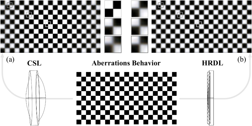
Figure 2: We summarize two aberrations behaviors for MOS: (a) Common Simple Lens (CSL), revealing spatial-variant degradation. (b) Hybrid Refractive Diffractive Lens (HRDL), revealing spatial-uniform degradation.

Although aberrations distributions of various optical systems are distinctly different, an summary of the commonalities and characteristics is necessary for a comprehensive and convincing benchmark for SSOA. For most MOS, the aberration distribution reveals two behaviors: spatial-variant degradation [7, 13, 38, 59] and spatial-uniform degradation [53, 54, 55, 42], which are relevant to the imaging principle of the optical components. To be specific, the Common Simple Lens (CSL) induces spatial-variant degradation, whereas the Hybrid Refractive Diffractive Lens (HRDL) induces spatial-uniform degradation.

Common simple lens. CSL often consists of optical elements with continuous surfaces [13, 7], i.e. spherical and aspherical surfaces. Due to refraction effects, the optical path varies with different thicknesses of the center and the edge FoVs, which ultimately leads to imaging results with spatial-variant degradation over different FoVs. As illustrated in Fig. 2(a), the image patch in the center of the FoV, which is associated with the paraxial region, is clear, while it degrades gradually with the increasing viewing angle.

Hybrid refractive diffractive lens. With the booming processing technology of micro- and nano precision optical components, Fresnel and DOE are applied in the design of MOS [14, 55]. The imaging principle of this type of MOS includes refraction and diffraction, called HRDL. HRDL enables a more uniform thickness-distribution of the optical elements, avoiding conspicuous differences in their optical path. In this sense, the aberrations of HRDL induce spatial-uniform degradation, i.e. the image patches at the center and edge viewing angles degrade similarly, shown in Fig. 2(b).

For image recovery in CI pipelines, the solutions to spatial-variant and spatial-uniform degradation are often different [7, 55]. Consequently, our established benchmark for SSOA is also divided accordingly based on the aberrations behaviors of CSL and HRDL.

3.2 Wave-based Imaging Simulation

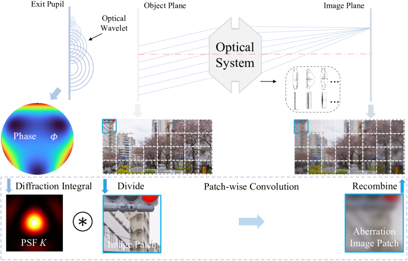
Figure 3: The simulation pipeline for constructing virtual prototype lens. The optical system is considered as a black box with phase function $\Phi$. We can simulate the imaging result of any MOS through the pipeline.

In learning-based CI pipelines, simulation [7] or live-shooting [55] is applied to generate data pairs for network training. When it comes to SSOA, imaging simulation appears as a more flexible solution to the acquisition of large-scale labeled data under various aberration distributions.

Considering the difficulty of ray-tracing between distinct components of different MOS, we view the imaging process in an abstract way. Applicable to most MOS, the modulation of the system on the incident wave phase is reflected in the phase function on its exit pupil plane. In other words, the specific structure of MOS can be abstracted into a black box, while the imaging process can be simulated only by modeling the phase function on exit pupil, i.e. wave-based imaging simulation.

To be specific, we apply Zernike polynomials [49] to describe the phase function of optical wavefronts $\Phi(x^{\prime},y^{\prime},\theta,\lambda)$ on exit pupil mathematically:

$$\Phi(x^{\prime},y^{\prime},\theta,\lambda)=\sum_{n,m}{C^{m}_{n}}(\theta,\lambda){Z^{m}_{n}}(x^{\prime},y^{\prime}),$$ (1)

where $C(\theta,\lambda)$ denotes Zernike coefficients under FoV $\theta$ and wavelength $\lambda$ and $Z$ refers to polynomials of the coordinate $(x^{\prime},y^{\prime})$ on exit pupil. The combination of different $m$ and $n$ represents different orders. For the specific expressions of each item, please refer to [49].

$\Phi(x^{\prime},y^{\prime},\theta,\lambda)$ represents the modulation of any MOS on incident light wave of $\theta$ and $\lambda$. It can be converted to Point Spread Function (PSF) $K(x,y,\theta,\lambda)$ on image plane through scalar diffraction integral [26] (detailed in the supplementary). In this way, we can simulate the imaging result of any MOS through patch-wise convolution [7] between the clear image and PSFs of different FoVs and wavelengths. The simulation pipeline is shown in Fig. 3.

3.3 Virtual Prototype Lens

We construct Virtual Prototype Lens (VPL) groups based on the proposed simulation pipeline to transform clear images to corrupted ones under various aberration distributions. To further investigate semantic segmentation under different severity of aberrations, we set up four aberration levels for CSL and HRDL respectively. The level is defined according to the shape (distribution of Zernike coefficients) and the kernel size (distribution of radius of spot diagram) of PSFs. Concretely, C1 to C4 are incremental levels for CSL, whereas an additional level C5 provides a hybrid set of C1 to C4 for comprehensive evaluation. Similarly, H1 to H5 are set for HRDL.

In detail, the curves of Zernike coefficients of different MOS samples, as a function of FoVs, are statistically analyzed, based on which we set the range and curve trend of Zernike coefficients for each level. In the same way, the random range of each aberration level for radius of spot diagram is also established. For detailed statistics, please refer to the supplementary material.

Supplied with the statistics, we generate random distributions of Zernike coefficients over $128$ normalized FoVs to describe the phase function in Eq. 1, i.e. different VPLs of CSL and HRDL. In the case of CSL (the same is true for HRDL), we produce five VPL samples for C1-C4 respectively and twenty samples for C5, where the samples in C5 are not duplicated with those in C1-C4. Hence, we can generate simulated results under different behaviors and levels of aberrations for any clear image, as shown in Fig. 1(a).

3.4 Benchmark Settings

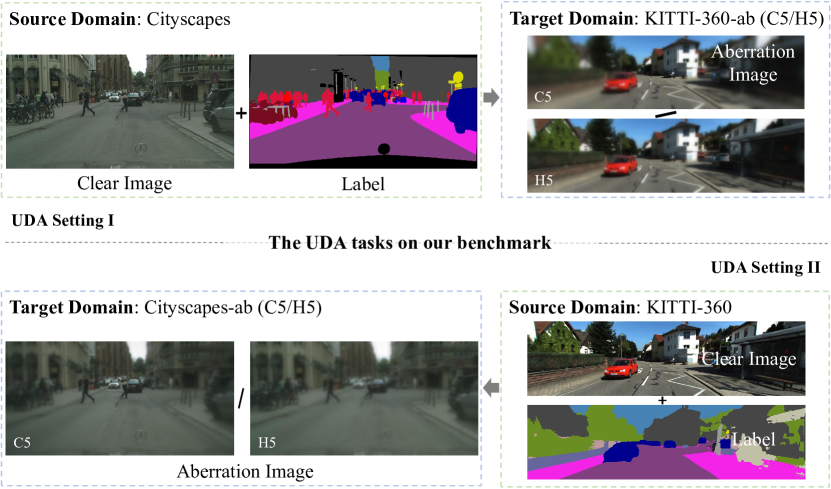
Figure 4: Illustration of the UDA tasks on our benchmark. We establish two settings to investigate SSOA without access to the labels of images with aberration.

Cityscapes [9] and KITTI-360 [41] are two semantic segmentation datasets with a large number of clear images and fine-annotated labels, where the categories and annotation methods are also consistent. In our work, we create Cityscapes-ab and KITTI-360-ab through our established VPL groups for benchmarking SSOA, which include labeled images under various aberration distributions.

The clear images from original datasets are imaged by VPL samples of C1-C5 and H1-H5, while the labels remain unchanged. The evaluation of semantic segmentation under different severity of aberrations is performed on the validation set of C1-C5 and H1-H5, where C5 and H5 may present comprehensive results. Considering the synthetic-to-real gap induced by simulation and adaptability to real MOS, the task of our benchmark follows unsupervised domain adaptive semantic segmentation. Specifically, as is shown in Fig. 4, UDA is performed on Cityscapes${\to}$KITTI-360-ab (C5/R5) and KITTI-360${\to}$Cityscapes-ab (C5/R5), which reflects real-world application scenarios where one cannot access the labels of corrupted images in an unseen domain taken by an unknown MOS.

In summary, our benchmark includes datasets under five levels of optical aberrations of two aberrations behaviors respectively. The performances of solutions to SSOA will be evaluated on our benchmark to measure the robustness and effectiveness of potential applications in semantic scene understanding with MOS.

4 Computational Imaging Assisted Domain Adaptation

In this section, we propose an UDA framework which transfers the knowledge of semantic segmentation under clear images and CI to SSOA, i.e. Computational Imaging Assisted Domain Adaptation (CIADA). CIADA explores to couple CI techniques with domain adaptive semantic segmentation via knowledge distillation, which we now detail.

4.1 Self-Training based UDA

With the goal of attaining relatively stable and high performance of UDA [22], self-training (ST) approaches [1, 27, 33, 36, 40, 82, 88] have achieved spectacular progress, where the model is gradually optimized via generated pseudo-labels. For our specific UDA task towards SSOA, we build up our baseline solution as a basic ST-UDA framework.

The encoder $E_{\Theta_{e}}$ and segmentation decoder $D_{\Theta_{s}}$ are trained with labeled source data of clear images $\mathcal{D}_{S}=\{{x_{S}}^{(i)},{y_{S}}^{(i)}\}_{i=1}^{N_{S}}$ and unlabeled target data of images with aberrations $\mathcal{D}_{T}=\{{x_{T}}^{(i)}\}_{i=1}^{N_{T}}$. A teacher network with encoder $E_{\Psi_{e}}$ and decoder $D_{\Psi_{s}}$ is applied to generate pseudo-labels ${y_{T}}_{pl}$ for target data. Our baseline follows the UDA training pipeline of [22], noted as ‘ST-UDA’ in this paper.

4.2 CIADA Architecture

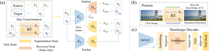
Figure 5: Our solution to unsupervised domain adaptive semantic segmentation under aberrations. (a) Overview of the CIADA architecture. We apply data transformation and auxiliary recovery task to distill the knowledge of CI. (b) Bidirectional Teacher (BT) for storing the knowledge of CI. (c) Network architecture of CIADA. Following [20], our decoder only aggregates last three stages of features from encoder. The features from ‘burger-in’, ‘burger-out’, and ‘align-out’ can be used to calculate the CD Loss.

For ST-UDA, the image degradation induced by aberrations of MOS leads to difficulty in the optimization of pseudo-labels. In other words, the domain gap is large, whereas the source knowledge seems to be insufficient.

We propose CIADA, pioneering to leverage the additional knowledge from image recovery of CI for assisting ST-UDA. The architecture of CIADA is shown in Fig. 5(a). The auxiliary task, namely self-training-based image recovery, is established for knowledge distillation.

Bidirectional teacher of computational imaging. The computational imaging for MOS, including simulation of imaging and image recovery, contains instructive knowledge of degradation characteristics to SSOA. We propose Bidirectional Teacher (BT), including a degradation network $g_{\phi}$ and a recovery network $g_{\psi}$, to store the knowledge of aberration-induced degradation from CI. BT is trained on ground-truth images and simulated images with aberrations based on optical parameters of applied MOS (Sec. 5.1). In Fig. 5(a)(b), the pretrained BT is applied for data transformation, producing augmented data $x_{S_{d}}$ for the source domain and pseudo-ground-truth $x_{T_{pgt}}$ for the target domain. Ultimately, we have the source dataset $\mathcal{D}_{S}{=}\{{x_{S}}^{(i)},{x_{S_{d}}}^{(i)},{y_{S}}^{(i)}\}_{i=1}^{N_{S}}$ and target dataset $\mathcal{D}_{T}{=}\{{x_{T_{pgt}}}^{(i)},{x_{T}}^{(i)},{{y_{T}}_{pl}}^{(i)}\}_{i=1}^{N_{T}}$ for CIADA training.

Network architecture. The network of CIADA contains a shared encoder $E_{\Theta_{e}}$, a decoder $D_{\Theta_{s}}$ for segmentation, and an auxiliary decoder $D_{\Theta_{r}}$ for image recovery, as shown in Fig. 5(a)(c). For segmentation against image degradation, we adopt the MiT encoder [74], which shows excellent zero-shot robustness on corrupted images, as $E_{\Theta_{e}}$. Meanwhile, considering the corruptions on local details of images induced by aberrations, the Hamburger decoder [15, 20] is applied for global information extraction in $D_{\Theta_{s}}$ and $D_{\Theta_{r}}$.

Correlation-based knowledge distillation. Considering the differences between high-level semantic segmentation and low-level image recovery, the single shared encoder architecture hinders the effective interaction of knowledge. In CIADA, we propose Correlation-based Knowledge Distillation to enhance the distillation process. We introduce the Correlation-based Distillation Loss function (CD Loss) to enforce segmenter $(E_{\Theta_{e}},D_{\Theta_{s}})$ to learn the degradation features extracted in recovery model $(E_{\Theta_{e}},D_{\Theta_{r}})$. To be specific, we calculate the self-correlation matrix $\mathcal{C}_{s,r}\in{W^{\prime}H^{\prime}{\times}H^{\prime}W^{\prime}}$ for feature maps ${{F}_{s,r}}\in{C^{\prime}{\times}H^{\prime}{\times}W^{\prime}}$ from decoder to model the associations among all pixels:

$$\mathcal{C}_{s,r}={(\frac{\mathcal{F}_{s,r}}{{\parallel}\mathcal{F}_{s,r}{\parallel}_{2}})^{T}}{\cdot}{(\frac{\mathcal{F}_{s,r}}{{\parallel}\mathcal{F}_{s,r}{\parallel}_{2}})},$$ (2)

and

$$\mathcal{F}_{s,r}=Reshape(Conv_{1\times 1}(F_{s,r})).\vspace{-0.5em}$$ (3)

where $\mathcal{F}_{s,r}\in{C^{\prime}{\times}H^{\prime}W^{\prime}}$ denotes the transformed feature map. The $1{\times}1$ convolution and $L_{2}$ norm are applied for stable training. Finally, the CD Loss is calculated based on the Charbonnier loss:

$$\mathcal{L}_{CD}(F_{s},F_{r})=\sqrt{{\parallel}\mathcal{C}_{s}-\mathcal{C}_{r}{\parallel}^{2}+\varepsilon^{2}},$$ (4)

where $\varepsilon$ is a constant value $10^{-3}$. The presented CD Loss regularizes features learned from high-level and low-level tasks, distilling the knowledge of how image degrades with aberrations to the segmenter.

4.3 Training Pipeline for CIADA

Based on the ST-UDA baseline, the joint self-training of semantic segmentation and image recovery on images with aberrations is utilized in CIADA:

Step0: Training of BT. BT ($g_{\phi},g_{\psi}$) is first trained for the generation of the degraded source image $x_{S_{d}}{=}g_{\phi}({x_{S}})$ and the recovered target image $x_{T_{pgt}}{=}g_{\psi}({x_{T}})$. Before CIADA training, the BT is pretrained, whereas the generation is performed online.

Step1: Joint training on source images. Labeled data $\{x_{S_{d}},{y_{S}}\}$ and paired degraded-clear images $\{x_{S_{d}},{x_{S}}\}$ are applied for source domain training. We use a combination loss function, composed of categorical Cross-Entropy (CE) loss for semantic segmentation $\mathcal{L}_{CE}$, Charbonnier loss for image recovery $\mathcal{L}_{Char}$, and the proposed CD Loss $\mathcal{L}_{{CD}}$, to supervise the training of the shared encoder architecture:

$$\begin{split}{\mathcal{L}}_{S}&=\mathcal{L}_{CE}(D_{\Theta_{s}}(E_{\Theta_{e}}(x_{S_{d}})),{y_{S}})\\ &+w_{1}\mathcal{L}_{Char}(D_{\Theta_{r}}(E_{\Theta_{e}}(x_{S_{d}})),{x_{S}})\\ &+w_{2}\mathcal{L}_{{CD}}({F_{s}},{F_{r}}).\end{split}$$ (5)

Step2: Generation of pseudo-labels. We generate pseudo-label ${y_{T}}_{pl}$ and pseudo weight $q_{T}$ for the target domain through the teacher segmenter $(E_{\Psi_{e}},D_{\Psi_{s}})$ in accordance with the ST-UDA baseline.

Step3: Joint training on target images. With pseudo-label $({y_{T}}_{pl},q_{T})$ and the pseudo-ground-truth image $x_{T_{pgt}}$, we jointly train the network on target data in a similar way:

$$\begin{split}{\mathcal{L}}_{T}&=w_{3}\mathcal{L}_{CE}(D_{\Theta_{s}}(E_{\Theta_{e}}(x_{T})),{q_{T}}{{y_{T}}_{pl}})\\ &+w_{4}\mathcal{L}_{Char}(D_{\Theta_{r}}(E_{\Theta_{e}}(x_{T})),x_{T_{pgt}})\\ &+w_{5}\mathcal{L}_{{CD}}({F_{s}},{F_{r}}).\end{split}$$ (6)

Step4: Training segmenter on mixed data. Class mixing [63] is applied to generate mixed data of both domains: $\{x_{M}=mix(x_{S_{d}},x_{T}),y_{M}=mix(y_{S},{q_{T}}{{y_{T}}_{pl}})\}$. The segmenter is trained as:

$${\mathcal{L}}_{M}=\mathcal{L}_{CE}(D_{\Theta_{s}}(E_{\Theta_{e}}(x_{M})),y_{M}).$$ (7)

In summary, the entire training objective is:

$${\mathcal{L}}=\mathcal{L}_{S}+\mathcal{L}_{T}+\mathcal{L}_{M}.$$ (8)

The $w_{1}$-$w_{5}$ in Eq. 5 and Eq. 6 are set as $0.05$, $1.00$, $0.01$, $0.05$, and $1.00$ for stable training empirically. In addition, we follow [22] to update the teacher segmenter for online pseudo-label generation via exponentially moving average [61]. The training pipeline for CIADA prompts the segmenter to learn how image degrades with aberrations from prior knowledge of CI and perform semantic segmentation on unseen images with optical aberrations.

5 Experiments

Table 1: Evaluation in mIoU(%) of state-of-the-art segmenters on our benchmark. We use segmenters properly trained only on clear Cityscapes from mmsegmentation [8] as KITTI-360 is seldom used for training. The validation images of Cityscapes are resized to $1024{\times}512$. Further implementation details are shown in the supplementary. We highlight the best and second best results.

	Cityscapes											KITTI-360
	Clear	CSL					HRDL					Clear	CSL					HRDL
	-	C1	C2	C3	C4	C5	H1	H2	H3	H4	H5	-	C1	C2	C3	C4	C5	H1	H2	H3	H4	H5
FCN [44]	75.44	74.57	73.23	68.08	37.93	63.20	74.63	73.13	67.40	19.36	52.99	46.44	45.63	42.88	32.80	14.73	31.28	45.64	42.61	27.71	05.02	29.81
PSPNet [83]	75.76	75.08	73.98	69.00	41.41	64.91	75.13	73.97	68.25	21.43	53.35	48.77	48.38	44.42	33.07	13.78	29.20	48.18	44.11	27.73	06.20	25.88
DeepLabV3+ [6]	77.11	76.65	75.43	70.03	44.18	66.50	76.64	75.32	69.18	20.84	54.80	50.38	49.87	47.67	35.50	14.34	31.08	49.65	47.19	29.78	02.22	26.97
SETR [84]	71.47	70.66	69.15	65.57	54.05	64.33	70.98	70.07	66.51	49.03	63.18	54.37	55.62	54.71	51.55	36.12	50.20	55.78	54.45	51.92	30.20	44.15
SegFormer [74]	78.04	77.00	75.37	69.20	50.12	67.73	77.26	76.06	68.88	43.67	65.55	59.81	59.03	55.99	45.68	27.25	43.67	57.83	53.55	45.97	17.97	42.01
SegNeXt [20]	79.07	78.62	77.05	70.03	47.98	66.99	78.56	77.01	70.12	37.60	62.93	56.30	53.75	52.07	40.55	18.91	36.52	54.06	51.51	37.01	08.38	30.55

Table 2: Comparison with state-of-the-art UDA methods.

	Road	S.walk	Build.	Wall	Fence	Pole	Tr.Light	Sign	Veget.	Terrain	Sky	Person	Rider	Car	Truck	Bus	Train	M.bike	Bike	mIoU
Cityscapes $\to$ KITTI-360-ab (C5)
CRST [88]	69.99	14.54	52.31	21.31	22.50	15.12	00.01	20.23	64.71	42.15	76.22	00.34	00.78	54.80	20.13	01.45	00.00	17.84	12.01	26.25
CLAN [47]	58.54	22.45	67.76	13.43	19.77	16.48	00.87	26.36	76.07	40.95	80.40	18.19	18.17	57.93	14.79	14.00	00.29	10.52	04.64	29.56
BDL [39]	64.38	32.16	68.06	18.13	21.72	13.33	00.09	11.59	75.56	44.77	81.37	06.51	02.70	66.36	23.27	17.10	00.01	24.94	05.32	30.39
DACS [63]	84.89	50.14	74.10	34.37	28.59	19.99	00.10	27.25	80.13	48.97	87.24	10.66	06.08	78.58	16.70	05.65	00.00	46.03	09.35	37.31
DAFormer [22]	74.54	38.99	78.44	33.46	34.98	23.91	00.66	38.66	80.54	46.03	88.01	42.33	23.83	82.19	54.09	38.07	23.63	42.37	27.39	45.90
HRDA [23]	60.10	30.12	80.65	41.74	35.63	19.41	00.43	39.17	78.70	39.67	88.96	27.74	10.40	78.80	58.51	40.40	03.91	43.42	23.63	42.18
CIADA (Ours)	84.23	47.30	79.31	38.86	33.07	22.45	00.85	38.70	81.69	47.62	87.34	47.60	28.09	83.14	56.32	39.01	40.46	54.39	24.15	49.19
Cityscapes $\to$ KITTI-360-ab (H5)
CRST [88]	64.34	14.58	48.60	21.18	21.93	17.79	00.00	19.37	62.40	44.35	64.69	0.20	12.96	47.51	10.02	10.42	00.00	12.71	16.66	25.77
CLAN [47]	57.76	18.58	63.59	10.85	19.99	15.59	00.35	23.04	72.61	40.74	73.56	13.27	30.03	53.20	05.59	50.81	00.72	08.33	13.22	30.10
BDL [39]	56.44	26.39	70.29	18.89	20.99	12.14	00.11	06.59	76.39	38.45	81.23	05.91	04.03	64.46	26.78	00.28	00.73	15.69	04.64	27.92
DACS [63]	68.82	35.04	73.51	26.57	28.40	21.29	00.03	29.71	80.09	54.27	83.96	24.97	17.71	77.53	21.79	56.81	00.91	26.03	19.71	39.32
DAFormer [22]	69.09	35.20	75.01	42.18	32.25	14.73	00.32	32.82	78.43	40.74	86.18	47.30	22.69	79.43	32.98	76.72	08.89	32.98	26.71	43.93
HRDA [23]	57.64	30.51	75.92	37.25	33.14	17.26	00.31	33.72	76.64	37.34	84.59	36.67	20.04	69.12	39.26	87.62	06.54	30.99	18.36	41.71
CIADA (Ours)	77.03	39.52	78.30	38.80	28.26	22.95	00.54	32.42	80.35	52.83	87.02	46.15	21.55	83.84	38.31	86.69	41.22	29.25	26.07	47.95

Table 3: Evaluation in mIoU(%) of possible solutions to semantic segmentation under different aberrations distributions.

	CSL					HRDL
	C1	C2	C3	C4	C5	H1	H2	H3	H4	H5
	Cs. $\to$ KI.-ab (C5)					Cs $\to$ KI.-ab (H5)
Oracle	59.98	56.80	53.32	43.93	53.57	59.25	58.34	50.57	40.06	55.62
Src-Only	52.15	49.84	38.77	19.11	37.60	52.76	49.96	35.47	11.49	36.91
ST-UDA	54.86	53.41	46.41	30.17	45.90	53.50	52.33	46.01	19.19	43.93
CIADA (Ours)	56.28	55.17	49.20	32.29	49.19	56.64	55.34	47.45	21.24	47.95
	KI. $\to$ Cs.-ab (C5)					KI. $\to$ Cs.-ab (H5)
Oracle	72.95	72.72	69.78	58.31	68.03	72.16	71.88	68.89	55.27	66.20
Src-Only	50.77	48.02	41.45	28.60	41.82	50.87	48.21	40.04	17.19	36.20
ST-UDA	58.71	58.08	55.34	45.61	54.49	60.21	59.23	55.47	35.38	51.89
CIADA (Ours)	60.24	59.97	57.79	49.11	56.77	60.59	60.20	57.56	45.58	55.37

5.1 Implementation Details

For brevity, all of the following settings are consistent for CSL and HRDL, and we will not discuss them separately. All the training processes of our work are implemented on a single NVIDIA GeForce RTX 3090.

Dataset for training BT. We select training/test dataset of $1922/447$ ground-truth images from Flickr2K [62], where images are resized to $512{\times}1024$. For target domain images taken by real MOS, the coarse aberration distribution is available through estimation or simulation [7, 85] based on the design parameters of the applied MOS. In our case, the MOS is VPL groups, whose parameters for PSF generation are known. To simulate the synthetic-to-real gap, we fine-tune the range of parameters and reconstruct other $20$ samples. We generate degraded images through reconstructed VPL groups for training the BT.

Dataset for optimizing UDA. In our benchmark, Cityscapes [9] ($2975/500$ images for training/validation set with a resolution of $2048{\times}1024$) and KITTI-360 [41] ($3063/768$ images for training/validation set with a resolution of $1408{\times}376$) are used as the source domain dataset, while the corresponding target domains are KITTI-360-ab and Cityscapes-ab, respectively. The frame rate of KITTI-360 is lowered $16$ times, to have a moderate size and maintain high scene diversity as the original samples are captured in suburbs, composed of sequences with insufficient scene variety. We resize images from Cityscapes to $1024{\times}512$ following a common practice [22].

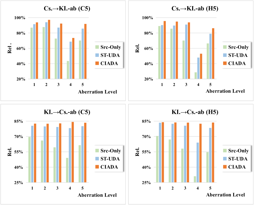
Figure 6: Relative performance (Rel., the normalized mIoU by oracle) of possible solutions to SSOA.

Training. We use NAFNet [5] for both degradation and recovery networks. The degradation- and the recovery network are trained separately. By default, we train BT in accordance with [5]. We follow [22] to train ST-UDA, with a batch size $2$ on random crops of $376{\times}376$ for $40K$ iterations. More training details are in the supplementary.

5.2 Influences of Optical Aberrations

Table 4: We conduct ablation studies to investigate why CIADA achieves superior SSOA result. The CD Loss is placed before task head in (b) considering different decoder architectures. In all cases, the experiments are implemented under Cityscapes${\to}$KITTI-360-ab (C5) and the model is evaluated on the validation set of KITTI-360-ab (C5) in mIoU ($\%$).

(a) Ablations on CI knowledge.

CIADA	Degradation	Recovery	mIOU
	-	-	45.07
	$\surd$	-	47.25
	-	$\surd$	47.24
	$\surd$	$\surd$	49.19
Compared Pipeline	Src-Only		37.60
	Cascade of CI&Seg		15.21

(b) Ablations on decoders.

Decoder	Src-Only	ST-UDA	CIADA
UperNet [72]	36.60	46.74	47.83
ASPP [6]	38.61	46.48	47.99
SegFormer [74]	37.60	45.11	46.37
DAFormer [22]	38.85	45.90	46.90
Hamburger∗ [20]	35.09	44.69	48.23
Hamburger [20]	36.40	45.07	48.55

(c) Ablations on the CD Loss.

Position of CD Loss	mIOU
w/o	48.20
burger-in	49.19
burger-out	49.01
align-out	48.55
all	48.71

The previous work [30] reveals that most segmenters are robust to aberration-based PSF blurs of conventional optical systems. However, the influences of much more severe aberrations of MOS have not been investigated. Based on our benchmark, we evaluate state-of-the-art segmenters in Tab. 1 under different behaviors and levels of optical aberrations. All the segmenters are robust to slight aberrations (C1/H1 and C2/H2) consistent with [30], but suffer considerable destructive effects when the aberration is severe, especially for level C4/H4 (${-}17.42{\sim}{-}48.18$ in mIoU). Compared to CNN-based models [44, 83, 6, 20], transformer-based segmenters [84, 74] are much more robust to aberrations which have higher mIoU under comprehensive sets of C5/H5 and severe aberrations sets of C4/H4, despite that the state-of-the-art CNN-based method [20] shows superior performance on clear images. In summary, for MOS whose aberrations are often severe, the influence of optical aberrations should be considered prudently for its applications in semantic segmentation. Further, the transformer architecture could be essential for SSOA with MOS due to its inherent robustness to image corruptions.

5.3 Comparison with State-of-the-Art Methods

UDA methods. Without access to labeled aberration images, UDA is a preferred solution to SSOA. Tab. 2 shows per-class results of previous UDA methods and our proposed CIADA under our UDA Setting I. All models are retrained on $376{\times}376$ random crops with a batch size of $2$ for $40K$ iterations. The transformer architecture proves to be crucial to SSOA for the considerable higher performance of DAFormer, HRDA, and CIADA. Moreover, compared to the state-of-the-art method [22], CIADA improves mIoU from $45.90$ to $49.19$ under CSL and $43.93$ to $47.95$ under HRDL due to the distillation of prior CI knowledge. Qualitative results are provided in the supplementary.

Possible solutions to SSOA. We evaluate possible solutions to SSOA based on our benchmark, i.e. oracle (trained with labeled target data), src-only (trained only with labeled source data), ST-UDA, and our proposed CIADA. SegFormer [74] is adopted for oracle and src-only training, while DAFormer [22] is applied for ST-UDA for their robustness and efficiency. Tab. 3 shows the mIoU of each solution under all behaviors and levels of aberrations. Taking oracle as the upper limit, we also show the relative performance in Fig. 6. For src-only methods, the performances drop dramatically as the aberration level becomes severer, while UDA methods (ST-UDA and CIADA) can bring impressive improvements. Moreover, CIADA proves to be a superior solution which outperforms ST-UDA baseline under all behaviors and levels aberrations, revealing the potential of domain adaptive SSOA with auxiliary CI pipelines.

5.4 Ablation Study

Ablations on CI knowledge. The CI knowledge of applied MOS is stored in the proposed bidirectional teacher. Tab. 4(c)(a) shows the results under different usages of BT. The single degradation teacher provides a mIoU increase of $2.18$ due to the data augmentation of aberrations, while the single recovery teacher improves the UDA performance by $2.17$ in mIoU through knowledge distillation of the auxiliary recovery in the target domain. However, the cascade of the recovery model and the src-only trained segmenter leads to a worse result ($37.60$ to $15.21$). The combination of two teachers achieves the highest gain of $4.12$, which enables auxiliary recovery learning in both domains.

Ablations on decoders. Tab. 4(c)(b) shows that the applied Hamburger decoder [20] achieves the best CIADA performance of $48.55$ in mIoU, despite with lower src-only and ST-UDA performance. Compared to the simple SegFormer decoder [74] or other decoders focusing on global context (i.e. UperNet [72], ASPP [6], and DAFormer [22]), the matrix-decomposition-based Hamburger can learn better global context in both semantic segmentation and image recovery [15], which is essential for CIADA with the auxiliary image recovery task. In addition, the Hamburger aggregating all encoder features (Hamburger^∗) brings a mIoU drop of $0.32$, showing that the shallow layer features hurt the performance of CIADA.

Ablations on the CD Loss. The CD Loss can be applied to any feature in the decoder, where we define burger-in, burger-out, and align-out for the Hamburger decoder in Fig. 5(c). As shown in Tab. 4(c)(c), the CD Loss brings improvements of $0.35{\sim}0.99$ due to the knowledge distillation between two tasks. The optimum position for the CD Loss is burger-in, which is far from the task head. It reveals the knowledge is best distilled at the early stage of the decoder due to the differences between the two tasks in CIADA.

6 Conclusion

In this paper, we look into Semantic Segmentation under Optical Aberrations (SSOA) via an unsupervised domain adaptation perspective. We put forward Virtual Prototype Lens (VPL) groups to generate datasets under different aberrations distributions for benchmarking SSOA. Additionally, the CIADA framework is proposed for robust SSOA with prior knowledge of CI. Our CIADA proves to be a superior solution which improves the state-of-the-art performance by $3.29/4.02$ and $2.28/3.48$ in mIoU in two UDA settings. We highlight that CIADA is a successful attempt to combine advanced CI techniques with SSOA without additional computation overhead during inference.

Supplementary Material

Appendix A Construction of Virtual Prototype Lens

We supplement the details of the construction of our Virtual Prototype Lens (VPL) in this section. In Section A.1, we illustrate the wave-based theory for imaging simulation of MOS. The statistics of MOS samples are detailed in Section A.2, based on which we generate our VPL groups in Section A.3.

A.1 Wave-based Imaging Simulation

Considering the complex and distinct structures of different MOS, we abstract the specific optical system into a black box. By calculating corresponding Point Spread Function (PSF) of each image patch under different Field of Views (FoVs), we can simulate the imaging result based on patch-wise convolution.

Without loss of generality, we take imaging system with circular pupil as a example, and firstly only discuss PSF calculation under a certain fixed FoV $\theta_{0}$ and wavelength $\lambda_{0}$. Assuming that a point light source is on the object plane, the corresponding intensity distribution on the image plane after propagation is the PSF.

Based on Fourier optics, the pupil function on pupil plane is modulated by aberrations. In this case, the effect of aberrations is to deviate the wavefront at the pupil from the ideal sphere. The wave aberration $W(x,y)$ is applied to represent the optical path difference between the two surfaces, so the phase function $\Phi(x,y)$ on the pupil plane is expressed as:

$$\Phi(x,y)=k_{0}W(x,y),$$ (9)

where $k_{0}=\frac{2\pi}{\lambda_{0}}$ denotes the wave number.

Zernike polynomial is a mathematical description of optical wavefronts propagating through circular pupils [49]. $\Phi$ can therefore be described by Zernike circle polynomials $\mathcal{W}(\rho,\theta)$ in polar coordinates as:

$$\Phi(\rho,\theta)=\mathcal{W}(\rho,\theta)=\sum_{n,m}{C^{m}_{n}}{Z^{m}_{n}}(\rho,\theta),$$ (10)

where $C$ denotes Zernike coefficients and $Z$ refers to polynomials. The combination of different $m$ and $n$ represents different orders. The above polar expression of $(\rho,\theta)$ can be rewritten in rectangular coordinates of $(x,y)$ by coordinate transformation ($x=\rho\cos\theta,y=\rho\sin\theta$).

With the phase function, the pupil function $\mathcal{P}(x,y)$ can be written by:

$$\mathcal{P}(x,y)=P(x,y)e^{\mathrm{i}\mathcal{W}(x,y)},$$ (11)

where $P(x,y)$ is circ function in our case.

In such imaging system, the light field propagating from the back surface to the image plane satisfies Fresnel diffraction theory and the amplitude can be calculated by scalar diffraction integral [26]. Before integral, we distinguish the coordinates of the image plane and the pupil plane: let the coordinate of the image plane be $(x,y)$ and that of the pupil plane be $(x^{\prime},y^{\prime})$. Therefore, the amplitude of the image plane $E(x,y)$ can be expressed as:

$$E(x,y)=\frac{E_{0}}{{\lambda_{0}}d}\iint\mathcal{P}(x^{\prime},y^{\prime})e^{-\mathrm{i}\frac{2\pi}{{\lambda_{0}}d}(x^{\prime}x+y^{\prime}y)}dx^{\prime}dy^{\prime},$$ (12)

where $E_{0}$ is a constant amplitude related to illumination, $d$ denotes the distance from the pupil plane to the image plane and $\lambda_{0}$ is the selected wavelength mentioned above.

The above discussion is carried out at a certain FoV $\theta_{0}$ and wavelength $\lambda_{0}$. In fact, the calculated $E$ on image plane is a function of FoV $\theta$ and wavelength $\lambda$. More generally, we write equation (12) as:

$$E(x,y,\theta,\lambda)=\frac{E_{0}}{{\lambda}d}\iint{\mathcal{P}(x^{\prime},y^{\prime},\theta,\lambda)e^{-\mathrm{i}\frac{2\pi}{{\lambda}d}(x^{\prime}x+y^{\prime}y)}dx^{\prime}dy^{\prime}}.$$ (13)

Finally, the focal intensity on the image plane is:

$$I(x,y,\theta,\lambda)={|E(x,y,\theta,\lambda)|^{2}}.$$ (14)

Under our hypothetical point light source condition, the above intensity is the PSF distribution $K(x,y,\theta,\lambda)$ required. In this way, we can get the degraded image patch $I_{ab}(x,y,\theta)$ at FoV $\theta$ induced by aberrations of MOS by:

$$I_{ab}(x,y,\theta)=\int{I_{clear}(x,y,\theta)\otimes K(x,y,\theta,\lambda)d\lambda},$$ (15)

where $I_{clear}(x,y,\theta)$ is the clear image patch and $\otimes$ denotes convolution.

A.2 Statistics Analysis of MOS Samples

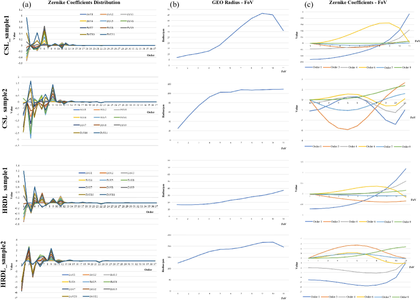
Figure S1: Statistics analysis of MOS samples. Considering the different FoVs of different MOS samples, we regularize the FoVs into $11$ normalized FoVs for all samples. (a) Distributions of Zernike coefficients under $11$ normalized FoVs. (b) Geometrical (GEO) radius distribution over FoVs. (c) Distributions of high impacts Zernike orders over normalized FoVs. The high impacts Zernike orders of MOS samples are: piston (Order1), $y$ tilt (Order3), defocus (Order4), $x$ primary astigmatism (Order6), $y$ primary coma (Order7), and $y$ trefoil (Order9), which are concluded from (a).

To generate virtual MOS samples for establishing the benchmark, we analyze the distribution of Zernike coefficients over FoVs and radius of spot diagram of different MOS samples, containing samples of Common Simple Lens (CSL) and Hybrid Refractive Diffractive Lens (HRDL). Fig. S1 shows the statistics results of two CSL samples and two HRDL samples, which can be used to determine the ranges and curve trends of random Zernike coefficients and kernel sizes of PSFs. Specifically, we conclude the Zernike orders of high values in Fig S1(a) and analyze the curve trends over FoVs of them in (c), establishing the random range of each high impact order and the type of corresponding curve fitting. Moreover, the GEO radius-FoV distributions in Fig. S1(b) are used for setting the size of PSF kernels of different levels and behaviors of aberrations. It reveals that the GEO radius distribution of HRDL is more uniform than CSL, which represents the spatial-uniform aberration behavior.

A.3 Settings of VPL groups

For comprehensive understanding how optical aberrations affect semantic segmentation, we establish different levels of aberrations distributions: C1-C4 for CSL and H1-H4 for HRDL based on above statistics. Additional levels C5 and H5 are hybrid sets of C1-C4 and H1-H4 respectively for an overall evaluation.

Tab. S1 shows the random ranges of parameters for constructing VPL groups. $(x,y)$ for Radius means the minimum GEO radius $x$ in the center FoV and maximum one $y$ in the edge FoV. The overall range $(-x,y)$ denotes that the max value of negative coefficients is $-x$ while $y$ is for positive ones. We generate random Zernike coefficients over $128$ normalized FoVs of each order according to its curve trend. Specifically, take one order for example, we first randomly select a possible curve trend which is concluded in statistics analysis. Then, a random number $r$ is generated among ranges $(x^{-},y^{-})/(x^{+},y^{+})$ in the last six columns of Tab. S1, where the former range is for negative values and the latter one is for positive values. In this way, the peak of the curve is calculated by the product of $r$ and overall range, based on which we fit the coefficients-FoV curves for all $37$ orders and generate a Zernike coefficients matrix of $37{\times}128$. Finally, the matrix which represents the aberrations distribution of one virtual MOS sample, i.e. the VPL sample, is used to calculate PSFs for imaging simulation.

Additionally, for a visualized understanding of our VPL samples and aberration levels, we show the imaging results of checkerboard of each level in Fig. S2. The average Zernike coefficients over FoVs and RGB channels of each level are also exhibited (including samples in level 5). Our VPL with the diverse aberrations distributions is a landmark engine for benchmarking SSOA.

Table S1: The ranges for random generation of GEO Radius (/${\mu}m$) and Zernike coefficients. All the random ranges are concluded from chosen MOS samples which ensure that the generated random distributions conform to the aberrations behaviors of most MOS as much as possible.

	Radius	Overall	Specific Orders
	-	-	1	3	4	6	7	9
C1	(5, 35)	(-0.4, 0.3)	(0.45, 1)/(0.8, 1)	(0.45, 1)/(0.45, 1)	(0.2, 0.5)/(0.3, 0.5)	(0.1, 0.5)/(0.2, 0.7)	(0.1, 0.35)/(0, 0.1)	(0.1, 0.15)/(0.1, 0.15)
C2	(5, 75)	(-0.7, 0.95)	(0.45, 1)/(0.8, 1)	(0.45, 1)/(0.45, 1)	(0.2, 0.5)/(0.3, 0.5)	(0.1, 0.5)/(0.2, 0.7)	(0.1, 0.35)/(0, 0.1)	(0.1, 0.15)/(0.1, 0.15)
C3	(5, 150)	(-3, 1.5)	(0.6, 1)/(0.8, 1)	(0.45, 1)/(0.45, 1)	(0.2, 0.5)/(0.3, 0.5)	(0.1, 0.25)/(0.1, 0.5)	(0.1, 0.2)/(0, 0.2)	(0.45, 0.6)/(0.45, 0.6)
C4	(5, 300)	(-6, 5)	(0.8, 1)/(0.8, 1)	(0.9, 1)/(0.9, 1)	(0.25, 0.7)/(0.4, 0.7)	(0.1, 0.15)/(0.1, 0.3)	(0.1, 0.15)/(0.2, 0.4)	(0.45, 0.8)/(0.45, 0.8)
H1	(15, 25)	(-0.3, 0.3)	(0.3, 0.8)/(0.75, 0.9)	(0.3, 0.8)/(0.6, 0.8)	(0.3, 0.4)/(0.35, 0.55)	(0.1, 0.3)/(0.4, 0.7)	(0.1, 0.2)/(0, 0.15)	(0.1, 0.15)/(0.1, 0.15)
H2	(15, 25)	(-0.6, 0.7)	(0.3, 0.8)/(0.75, 0.9)	(0.3, 0.8)/(0.6, 0.8)	(0.3, 0.4)/(0.35, 0.55)	(0.1, 0.3)/(0.4, 0.7)	(0.1, 0.2)/(0, 0.15)	(0.1, 0.15)/(0.1, 0.15)
H3	(70, 100)	(-2.5, 2)	(0.6, 0.8)/(0.75, 0.9)	(0.3, 0.8)/(0.6, 0.8)	(0.4, 0.6)/(0.45, 0.65)	(0.1, 0.25)/(0.3, 0.5)	(0.1, 0.15)/(0.1, 0.2)	(0.45, 0.65)/(0.45, 0.6)
H4	(160, 200)	(-6, 5)	(0.75, 0.8)/(0.75, 0.9)	(0.9, 1)/(0.8, 0.9)	(0.25, 0.6)/(0.4, 0.75)	(0.1, 0.25)/(0.2, 0.4)	(0.1, 0.15)/(0.3, 0.4)	(0.65, 0.8)/(0.45, 0.6)

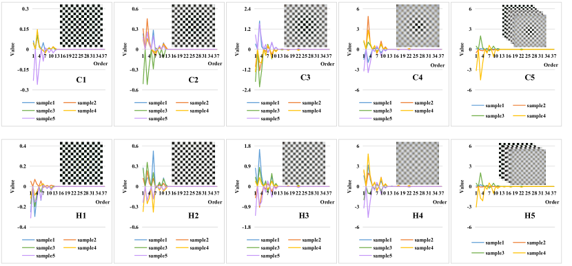
Figure S2: Average Zernike coefficients distributions over FoVs and RGB channels of different samples for each level. We also show the imaging results of checkerboard of each level. In C5 and H5, we select $4$ samples of different levels for example. Our VPL groups contain diverse aberrations distributions which are significant for benchmarking SSOA.

Appendix B Further Results for CIADA

In this section, we supplement the implementation details of all experiments and provide the qualitative results of possible solutions to SSOA. The settings and aberrations distributions of VPL samples in BT are provided in Section B.1. We illustrate the training and evaluation settings of all related methods in Section B.2, while the qualitative results of evaluated possible solutions are in Section B.3.

B.1 Datasets for Bidirectional Teacher

Considering the potential synthetic-to-real gap where the simulated imaging result are often different from that of real MOS due to manufacture, the accurate PSFs of applied MOS are often unavailable for generating synthetic aberration images for CI training. In other words, the calculated PSFs based on design parameters of MOS often deviate from the real ones. In the case of our VPL samples, to simulate the gap, we should fine-tune the parameters and reconstruct other $20$ VPL samples different from those in our benchmark, for datasets generation of BT training. Tab. S2 and Fig. S3 show the random ranges and average Zernike coefficient distributions of VPL samples for BT training. Compared to those in Tab. S1 and Fig S2, the fine-tuned parameters ensure that the aberration distribution deviates from the actual one of applied VPL samples, but with a similar behavior and level for the effectiveness of stored prior CI knowledge.

Table S2: The fine-tuned ranges for generation of VPL samples used in BT training. The random ranges of mentioned specific orders remain unchanged for similar aberration distribution.

	Radius	Overall		Radius	Overall
BT-C1	(5, 45)	(-0.45, 0.35)	BT-H1	(20, 30)	(-0.4, 0.4)
BT-C2	(10, 75)	(-0.6, 1)	BT-H2	(25, 40)	(-0.7, 0.7)
BT-C3	(15, 155)	(-3.5, 2)	BT-H3	(85, 115)	(-3, 2.5)
BT-C4	(15, 255)	(-6, 6)	BT-H4	(150, 185)	(-6, 6)

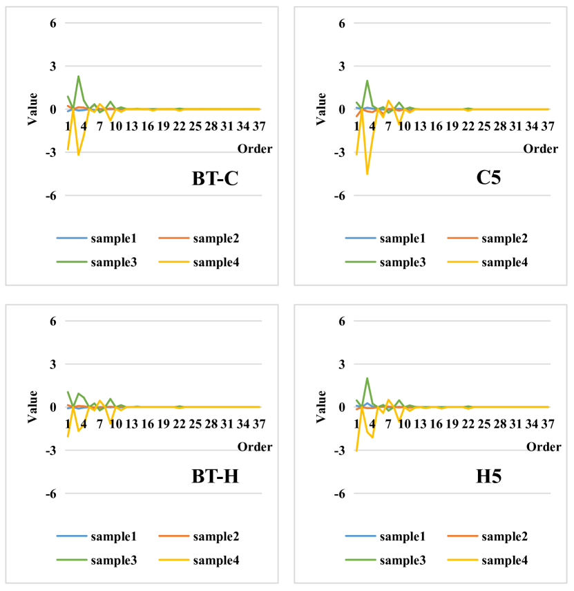
Figure S3: Average Zernike coefficient distributions over FoVs and RGB channels. We compare the selected 4 samples for BT training (BT-C and BT-H) with those for our benchmark (C5 and H5). The different aberration distributions simulate the synthetic-to-real gap.

Table S3: Implementation details of evaluated segmenters. We detail the configurations which are available in mmsegmentation [8] and  [20].

Method	Backbone	Decoder	Crop size	Testing size (Cs.)	Testing size (KI.)	Iterations	Configuration
FCN [44]	ResNet101	FCNHead	$512\times 1024$	$512\times 1024$	$376\times 1408$	$80K$	fcn_r101-d8_fp16_512x1024_80k_cityscapes
PSPNet [83]	ResNet101	PSPHead	$512\times 1024$	$512\times 1024$	$376\times 1408$	$80K$	pspnet_r101-d8_512x1024_80k_cityscapes
DeepLabV3+ [6]	ResNet101	ASPPHead	$512\times 1024$	$512\times 1024$	$376\times 1408$	$80K$	deeplabv3plus_r101-d8_512x1024_80k_cityscapes
SETR [84]	ViT	SETRUPHead	$768\times 768$	$512\times 1024$	$376\times 1408$	$80K$	setr_vit-large_pup_8x1_768x768_80k_cityscapes
SegFormer [74]	MiT-b5	SegFormerHead	$1024\times 1024$	$512\times 1024$	$376\times 1408$	$160K$	segformer.b5.1024x1024.city.160k
SegNeXt [20]	MSCAN	LightHamHead	$1024\times 1024$	$512\times 1024$	$376\times 1408$	$160K$	segnext.large.1024x1024.city.160k

B.2 Implementation Details

Training of BT. We apply NAFNet [5] for both image recovery network and image degradation network in BT for its efficient and effective performance in low-level vision. The two networks in BT are trained separately for recovery of target images and degradation of source images. The width and depth of applied NAFNet are $32$ and $[1,1,1,28]$. Based on BasicSR [67], in accordance with [5], we train BT with AdamW [46] for $160K$ iterations with an initial learning rate of $1e^{-3}$, which is gradually reduced to $1e^{-6}$ with the cosine annealing schedule [45], on image patches of $256{\times}256$ with a batch size of $8$.

Training of CIADA. We adopt MiT-b5 [74] with a feature pyramid of $[64,128,320,512]$ for the encoder, and Hamburger [20] which aggregates last three stages of features with $C{=}512$ for both the semantic segmentation decoder and the auxiliary recovery decoder. Following [22] and [63], we set $T{=}0.01$ for RCS temperature, $r{=}0.75$ and $\lambda_{FD}{=}0.005$ for FD, $\alpha{=}0.99$, and $\tau{=}0.968$ for data mixing. CIADA is trained with AdamW for $40K$ iterations with a learning rate of $6e^{-5}$ for the encoder and $6e^{-4}$ for the decoder, where weight decay of $0.01$ and a linear learning rate warmup of $1.5K$ iterations are applied. We train it with a batch size of $2$ on two $376{\times}376$ random crops based on mmsegmenmtation [8].

Evaluation of state-of-the-art segmenters. In Tab. S3, we show the details of each evaluated segmenters. All settings and codes are available in mmsegmentation [8] and [20].

Evaluation of possible solutions to SSOA. SegFormer-b5 [74] is adopted for oracle and src-only methods. We train it with the same settings as our CIADA for a fair comparison. Additionally, DAFormer [22] is chosen as the baseline of ST-UDA which is trained under its default setting except that the crop size is changed from $512{\times}512$ to $376{\times}376$ considering the resolution of KITTI-360 [41] ($376{\times}1408$).

B.3 Qualitative Results

The qualitative results of possible solutions to SSOA on Cityscapes${\to}$KITTI-360-ab (C5), Cityscapes${\to}$KITTI-360-ab (H5), KITTI-360${\to}$Cityscapes-ab (C5), and KITTI-360${\to}$Cityscapes-ab (H5) are shown in Figs. S4, S5, S6 and S7, respectively. We note that some special classes of ground truth are not considered during the training process as a common practice [22, 23].

The catastrophic results of the src-only method reveal that the optical aberrations, especially the severe aberrations of MOS, bring considerable damages to semantic segmentation, which prevents the applications of MOS in scene understanding. ST-UDA, as a baseline method which adapts the segmenter to unseen aberration images, improves the segmentation results significantly, where most of the classes in the scene can be understood roughly. However, there exists terrible noises in its segmentation results and the segmentation of each instance is incoherent, especially at the junction of instances. CIADA proves to be a superior solution to SSOA, whose results are relative clean, coherent, and accurate. The usage of CI knowledge helps the segmenter in CIADA learn how the image degrades, which is essential to SSOA.

The qualitative results also reveal some limitations of CIADA. Many sidewalks are neglected or confused with roads due to the corrupted textures. Moreover, because of diverse aberration distributions of VPL samples, the BT can only produce coarse recovery results of the target images whose textures and details remain unclear. Consequently, the limitation leads to the failure of CIADA in some fine marginal detail distinctions.

Appendix C Discussion

C.1 Limitations

Our work appears to be a landmark for investigating the applications of MOS in semantic scene understanding. It is the first work to address semantic segmentation under severe optical aberrations of MOS to the best of our knowledge. However, some limitations require to be further explored for more robust results.

First and foremost, there remains considerable improvement space in the performance of solutions to SSOA, both in mIoU and qualitative results. CIADA and ST-UDA can make the segmenter successfully understand the scene roughly under aberrations, but the results of details, especially the joint of some adjacent instances, are unsatisfactory, which make it disadvantageous for applications of MOS in semantic scene understanding. To deal with the tough task, we believe that more stages and iterations of training with a larger batch size is worth trying for reaching robust performance. Moreover, the network architecture of BT should be further investigated for a better storage of CI knowledge, which is proved to be essential to the task.

Additionally, all the aberration images in our benchmark are simulated by optical models. Despite that we set our task as unsupervised domain adaptation and artificially simulate the potential synthetic-to-real gap in BT through fine-tuning the parameters, the performance of our model on real MOS may also be different from our experiment results on the benchmark. We will try to capture real aberration images by different MOS samples with fine annotations for a more convincing benchmark in our future work.

Last but not least, the statistics analysis of MOS samples for the constructions of VPL needs to be further improved. We will collect more samples in our analysis, to make a comprehensive summary of aberration distributions of MOS. Smoother gradation of aberration levels and more diverse aberration distributions will also be considered in the future improvements of our benchmark.

C.2 Potential Negative Impact

We explore the potential applications of MOS in semantic scene understanding, which is valuable for the development of various mobile and wearable devices, such as intelligent robots, intelligent monitoring, and AR/VR equipment. However, the advantage of tiny size of MOS may also be leveraged for military reconnaissance and sneak shot. We hope that the applications of MOS can be regularized by laws to benefit our world.

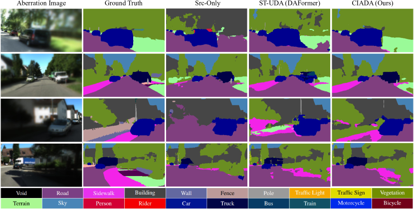
Figure S4: Qualitative results on Cityscapes${\to}$KITTI-360-ab (C5).

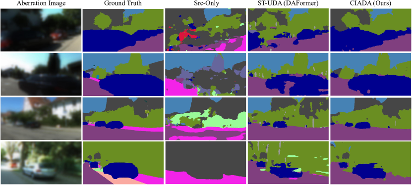
Figure S5: Qualitative results on Cityscapes${\to}$KITTI-360-ab (H5).

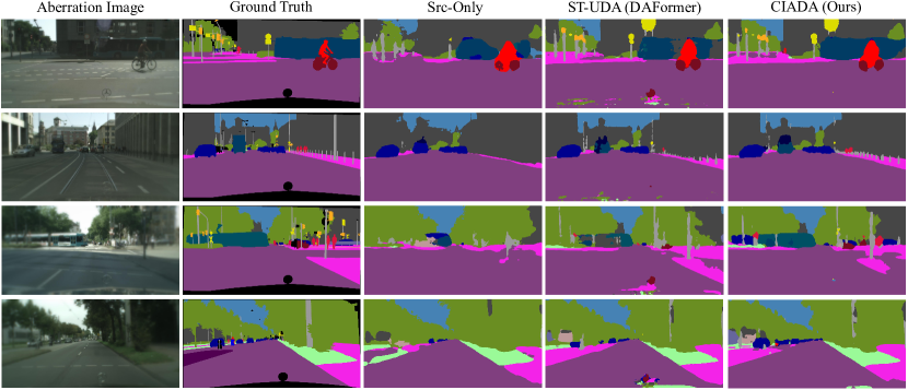
Figure S6: Qualitative results on KITTI-360${\to}$Cityscapes-ab (C5).

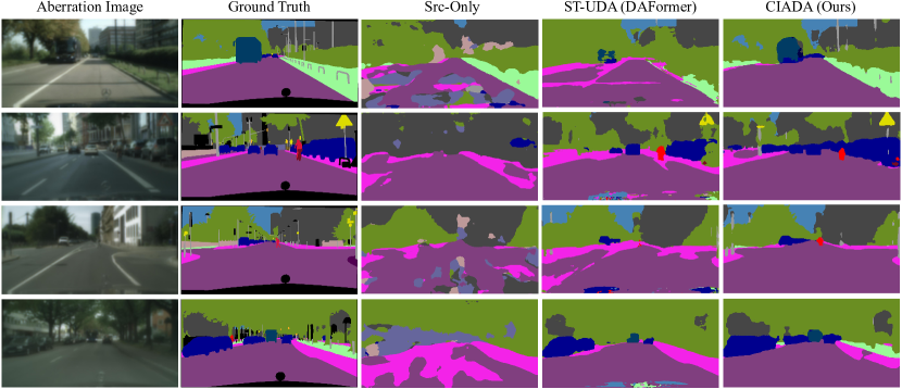
Figure S7: Qualitative results on KITTI-360${\to}$Cityscapes-ab (H5).

References

- [1] Nikita Araslanov and Stefan Roth. Self-supervised augmentation consistency for adapting semantic segmentation. In CVPR, 2021.
- [2] George Barbastathis, Aydogan Ozcan, and Guohai Situ. On the use of deep learning for computational imaging. Optica, 2019.
- [3] David Bruggemann, Christos Sakaridis, Prune Truong, and Luc Van Gool. Refign: Align and refine for adaptation of semantic segmentation to adverse conditions. In WACV, 2023.
- [4] Wei-Lun Chang, Hui-Po Wang, Wen-Hsiao Peng, and Wei-Chen Chiu. All about structure: Adapting structural information across domains for boosting semantic segmentation. In CVPR, 2019.
- [5] Liangyu Chen, Xiaojie Chu, Xiangyu Zhang, and Jian Sun. Simple baselines for image restoration. arXiv preprint arXiv:2204.04676, 2022.
- [6] Liang-Chieh Chen, Yukun Zhu, George Papandreou, Florian Schroff, and Hartwig Adam. Encoder-decoder with atrous separable convolution for semantic image segmentation. In ECCV, 2018.
- [7] Shiqi Chen, Huajun Feng, Dexin Pan, Zhihai Xu, Qi Li, and Yueting Chen. Optical aberrations correction in postprocessing using imaging simulation. TOG, 2021.
- [8] MMSegmentation Contributors. MMSegmentation: OpenMMLab semantic segmentation toolbox and benchmark. https://github.com/open-mmlab/mmsegmentation, 2020.
- [9] Marius Cordts, Mohamed Omran, Sebastian Ramos, Timo Rehfeld, Markus Enzweiler, Rodrigo Benenson, Uwe Franke, Stefan Roth, and Bernt Schiele. The cityscapes dataset for semantic urban scene understanding. In CVPR, 2016.
- [10] Xueqing Deng, Peng Wang, Xiaochen Lian, and Shawn Newsam. NightLab: A dual-level architecture with hardness detection for segmentation at night. In CVPR, 2022.
- [11] Xiong Dun, Hayato Ikoma, Gordon Wetzstein, Zhanshan Wang, Xinbin Cheng, and Yifan Peng. Learned rotationally symmetric diffractive achromat for full-spectrum computational imaging. Optica, 2020.
- [12] Huan Gao, Jichang Guo, Guoli Wang, and Qian Zhang. Cross-domain correlation distillation for unsupervised domain adaptation in nighttime semantic segmentation. In CVPR, 2022.
- [13] Shaohua Gao, Lei Sun, Qi Jiang, Hao Shi, Jia Wang, Kaiwei Wang, and Jian Bai. Compact and lightweight panoramic annular lens for computer vision tasks. OE, 2022.
- [14] Shaohua Gao, Kailun Yang, Hao Shi, Kaiwei Wang, and Jian Bai. Review on panoramic imaging and its applications in scene understanding. TIM, 2022.
- [15] Zhengyang Geng, Meng-Hao Guo, Hongxu Chen, Xia Li, Ke Wei, and Zhouchen Lin. Is attention better than matrix decomposition? In ICLR, 2021.
- [16] Rui Gong, Yuhua Chen, Danda Pani Paudel, Yawei Li, Ajad Chhatkuli, Wen Li, Dengxin Dai, and Luc Van Gool. Cluster, split, fuse, and update: Meta-learning for open compound domain adaptive semantic segmentation. In CVPR, 2021.
- [17] Ian Goodfellow, Jean Pouget-Abadie, Mehdi Mirza, Bing Xu, David Warde-Farley, Sherjil Ozair, Aaron Courville, and Yoshua Bengio. Generative adversarial networks. Communications of the ACM, 2020.
- [18] Tianrui Guan, Divya Kothandaraman, Rohan Chandra, Adarsh Jagan Sathyamoorthy, Kasun Weerakoon, and Dinesh Manocha. GA-Nav: Efficient terrain segmentation for robot navigation in unstructured outdoor environments. RA-L, 2022.
- [19] Dazhou Guo, Yanting Pei, Kang Zheng, Hongkai Yu, Yuhang Lu, and Song Wang. Degraded image semantic segmentation with dense-gram networks. TIP, 2020.
- [20] Meng-Hao Guo, Cheng-Ze Lu, Qibin Hou, Zhengning Liu, Ming-Ming Cheng, and Shi-Min Hu. SegNeXt: Rethinking convolutional attention design for semantic segmentation. In NeurIPS, 2022.
- [21] Judy Hoffman, Eric Tzeng, Taesung Park, Jun-Yan Zhu, Phillip Isola, Kate Saenko, Alexei Efros, and Trevor Darrell. CyCADA: Cycle-consistent adversarial domain adaptation. In ICML, 2018.
- [22] Lukas Hoyer, Dengxin Dai, and Luc Van Gool. DAFormer: Improving network architectures and training strategies for domain-adaptive semantic segmentation. In CVPR, 2022.
- [23] Lukas Hoyer, Dengxin Dai, and Luc Van Gool. HRDA: Context-aware high-resolution domain-adaptive semantic segmentation. In ECCV, 2022.
- [24] Xia Hua, Yujie Wang, Shuming Wang, Xiujuan Zou, You Zhou, Lin Li, Feng Yan, Xun Cao, Shumin Xiao, Din Ping Tsai, Jiecai Han, Zhenlin Wang, and Shining Zhu. Ultra-compact snapshot spectral light-field imaging. NC, 2022.
- [25] Jiaxing Huang, Shijian Lu, Dayan Guan, and Xiaobing Zhang. Contextual-relation consistent domain adaptation for semantic segmentation. In ECCV, 2020.
- [26] Elisha Huggins. Introduction to fourier optics. The Physics Teacher, 2007.
- [27] Xinyue Huo, Lingxi Xie, Hengtong Hu, Wengang Zhou, Houqiang Li, and Qi Tian. Domain-agnostic prior for transfer semantic segmentation. In CVPR, 2022.
- [28] Qi Jiang, Hao Shi, Lei Sun, Shaohua Gao, Kailun Yang, and Kaiwei Wang. Annular computational imaging: Capture clear panoramic images through simple lens. arXiv preprint arXiv:2206.06070, 2022.
- [29] Zhengkai Jiang, Yuxi Li, Ceyuan Yang, Peng Gao, Yabiao Wang, Ying Tai, and Chengjie Wang. Prototypical contrast adaptation for domain adaptive semantic segmentation. In ECCV, 2022.
- [30] Christoph Kamann and Carsten Rother. Benchmarking the robustness of semantic segmentation models. In CVPR, 2020.
- [31] Christoph Kamann and Carsten Rother. Increasing the robustness of semantic segmentation models with painting-by-numbers. In ECCV, 2020.
- [32] Guoliang Kang, Yunchao Wei, Yi Yang, Yueting Zhuang, and Alexander Hauptmann. Pixel-level cycle association: A new perspective for domain adaptive semantic segmentation. In NeurIPS, 2020.
- [33] Xin Lai, Zhuotao Tian, Xiaogang Xu, Yingcong Chen, Shu Liu, Hengshuang Zhao, Liwei Wang, and Jiaya Jia. DecoupleNet: Decoupled network for domain adaptive semantic segmentation. In ECCV, 2022.
- [34] Geon Lee, Chanho Eom, Wonkyung Lee, Hyekang Park, and Bumsub Ham. Bi-directional contrastive learning for domain adaptive semantic segmentation. In ECCV, 2022.
- [35] Guangrui Li, Guoliang Kang, Wu Liu, Yunchao Wei, and Yi Yang. Content-consistent matching for domain adaptive semantic segmentation. In ECCV, 2020.
- [36] Ruihuang Li, Shuai Li, Chenhang He, Yabin Zhang, Xu Jia, and Lei Zhang. Class-balanced pixel-level self-labeling for domain adaptive semantic segmentation. In CVPR, 2022.
- [37] Shuang Li, Binhui Xie, Bin Zang, Chi Harold Liu, Xinjing Cheng, Ruigang Yang, and Guoren Wang. Semantic distribution-aware contrastive adaptation for semantic segmentation. arXiv preprint arXiv:2105.05013, 2021.
- [38] Xiu Li, Jinli Suo, Weihang Zhang, Xin Yuan, and Qionghai Dai. Universal and flexible optical aberration correction using deep-prior based deconvolution. In ICCV, 2021.
- [39] Yunsheng Li, Lu Yuan, and Nuno Vasconcelos. Bidirectional learning for domain adaptation of semantic segmentation. In CVPR, 2019.
- [40] Qing Lian, Fengmao Lv, Lixin Duan, and Boqing Gong. Constructing self-motivated pyramid curriculums for cross-domain semantic segmentation: A non-adversarial approach. In ICCV, 2019.
- [41] Yiyi Liao, Jun Xie, and Andreas Geiger. KITTI-360: A novel dataset and benchmarks for urban scene understanding in 2D and 3D. TPAMI, 2022.
- [42] Kai Liu, Xiao Yu, Yongsen Xu, Yulei Xu, Yuan Yao, Nan Di, Yefei Wang, Hao Wang, and Honghai Shen. Computational imaging for simultaneous image restoration and super-resolution image reconstruction of single-lens diffractive optical system. Applied Sciences, 2022.
- [43] Yahao Liu, Jinhong Deng, Xinchen Gao, Wen Li, and Lixin Duan. BAPA-Net: Boundary adaptation and prototype alignment for cross-domain semantic segmentation. In ICCV, 2021.
- [44] Jonathan Long, Evan Shelhamer, and Trevor Darrell. Fully convolutional networks for semantic segmentation. In CVPR, 2015.
- [45] Ilya Loshchilov and Frank Hutter. SGDR: Stochastic gradient descent with warm restarts. In ICLR, 2017.
- [46] Ilya Loshchilov and Frank Hutter. Decoupled weight decay regularization. In ICLR, 2019.
- [47] Yawei Luo, Liang Zheng, Tao Guan, Junqing Yu, and Yi Yang. Taking a closer look at domain shift: Category-level adversaries for semantics consistent domain adaptation. In CVPR, 2019.
- [48] Haoyu Ma, Xiangru Lin, Zifeng Wu, and Yizhou Yu. Coarse-to-fine domain adaptive semantic segmentation with photometric alignment and category-center regularization. In CVPR, 2021.
- [49] Virendra N. Mahajan. Zernike circle polynomials and optical aberrations of systems with circular pupils. AO, 1994.
- [50] Ondrej Miksik, Vibhav Vineet, Morten Lidegaard, Ram Prasaath, Matthias Nießner, Stuart Golodetz, Stephen L. Hicks, Patrick Pérez, Shahram Izadi, and Philip H. S. Torr. The semantic paintbrush: Interactive 3D mapping and recognition in large outdoor spaces. In CHI, 2015.
- [51] Fei Pan, Inkyu Shin, Francois Rameau, Seokju Lee, and In So Kweon. Unsupervised intra-domain adaptation for semantic segmentation through self-supervision. In CVPR, 2020.
- [52] Yanting Pei, Yaping Huang, Qi Zou, Xingyuan Zhang, and Song Wang. Effects of image degradation and degradation removal to CNN-based image classification. TPAMI, 2021.
- [53] Yifan Peng, Qiang Fu, Hadi Amata, Shuochen Su, Felix Heide, and Wolfgang Heidrich. Computational imaging using lightweight diffractive-refractive optics. Optics Express, 2015.
- [54] Yifan Peng, Qiang Fu, Felix Heide, and Wolfgang Heidrich. The diffractive achromat full spectrum computational imaging with diffractive optics. TOG, 2016.
- [55] Yifan Peng, Qilin Sun, Xiong Dun, Gordon Wetzstein, Wolfgang Heidrich, and Felix Heide. Learned large field-of-view imaging with thin-plate optics. TOG, 2019.
- [56] Eduardo Romera, José M. Alvarez, Luis M. Bergasa, and Roberto Arroyo. ERFNet: Efficient residual factorized ConvNet for real-time semantic segmentation. T-ITS, 2018.
- [57] Eduardo Romera, Luis M. Bergasa, Kailun Yang, Jose M. Alvarez, and Rafael Barea. Bridging the day and night domain gap for semantic segmentation. In IV, 2019.
- [58] Christos Sakaridis, Dengxin Dai, and Luc Van Gool. ACDC: The adverse conditions dataset with correspondences for semantic driving scene understanding. In ICCV, 2021.
- [59] Christian J Schuler, Michael Hirsch, Stefan Harmeling, and Bernhard Schölkopf. Non-stationary correction of optical aberrations. In ICCV, 2011.
- [60] Prabhu Teja Sivaprasad and François Fleuret. Uncertainty reduction for model adaptation in semantic segmentation. In CVPR, 2021.
- [61] Antti Tarvainen and Harri Valpola. Mean teachers are better role models: Weight-averaged consistency targets improve semi-supervised deep learning results. In NeurIPS, 2017.
- [62] Radu Timofte, Eirikur Agustsson, Luc Van Gool, Ming-Hsuan Yang, Lei Zhang, Bee Lim, Sanghyun Son, Heewon Kim, Seungjun Nah, Kyoung Mu Lee, Xintao Wang, Yapeng Tian, Ke Yu, Yulun Zhang, Shixiang Wu, Chao Dong, Liang Lin, Yu Qiao, Chen Change Loy, Woong Bae, Jae Jun Yoo, Yoseob Han, Jong Chul Ye, Jae-Seok Choi, Munchurl Kim, Yuchen Fan, Jiahui Yu, Wei Han, Ding Liu, Haichao Yu, Zhangyang Wang, Honghui Shi, Xinchao Wang, Thomas S. Huang, Yunjin Chen, Kai Zhang, Wangmeng Zuo, Zhimin Tang, Linkai Luo, Shaohui Li, Min Fu, Lei Cao, Wen Heng, Giang Bui, Truc Le, Ye Duan, Dacheng Tao, Ruxin Wang, Xu Lin, Jianxin Pang, Jinchang Xu, Yu Zhao, Xiangyu Xu, Jin-shan Pan, Deqing Sun, Yujin Zhang, Xibin Song, Yuchao Dai, Xueying Qin, Xuan-Phung Huynh, Tiantong Guo, Hojjat Seyed Mousavi, Tiep Huu Vu, Vishal Monga, Cristóvão Cruz, Karen O. Egiazarian, Vladimir Katkovnik, Rakesh Mehta, Arnav Kumar Jain, Abhinav Agarwalla, Ch V. Sai Praveen, Ruofan Zhou, Hongdiao Wen, Che Zhu, Zhiqiang Xia, Zhengtao Wang, and Qi Guo. NTIRE 2017 challenge on single image super-resolution: Methods and results. In CVPRW, 2017.
- [63] Wilhelm Tranheden, Viktor Olsson, Juliano Pinto, and Lennart Svensson. DACS: Domain adaptation via cross-domain mixed sampling. In WACV, 2021.
- [64] Yi-Hsuan Tsai, Wei-Chih Hung, Samuel Schulter, Kihyuk Sohn, Ming-Hsuan Yang, and Manmohan Chandraker. Learning to adapt structured output space for semantic segmentation. In CVPR, 2018.
- [65] Rosaura G. VidalMata, Sreya Banerjee, Brandon RichardWebster, Michael Albright, Pedro Davalos, Scott McCloskey, Ben Miller, Asong Tambo, Sushobhan Ghosh, Sudarshan Nagesh, Ye Yuan, Yueyu Hu, Junru Wu, Wenhan Yang, Xiaoshuai Zhang, Jiaying Liu, Zhangyang Wang, Hwann-Tzong Chen, Tzu-Wei Huang, Wen-Chi Chin, Yi-Chun Li, Mahmoud Lababidi, Charles Otto, and Walter J. Scheirer. Bridging the gap between computational photography and visual recognition. TPAMI, 2021.
- [66] Tuan-Hung Vu, Himalaya Jain, Maxime Bucher, Matthieu Cord, and Patrick Pérez. ADVENT: Adversarial entropy minimization for domain adaptation in semantic segmentation. In CVPR, 2019.
- [67] Xintao Wang, Liangbin Xie, Ke Yu, Kelvin C.K. Chan, Chen Change Loy, and Chao Dong. BasicSR: Open source image and video restoration toolbox. https://github.com/XPixelGroup/BasicSR, 2022.
- [68] Yuxi Wang, Junran Peng, and ZhaoXiang Zhang. Uncertainty-aware pseudo label refinery for domain adaptive semantic segmentation. In ICCV, 2021.
- [69] Zhonghao Wang, Mo Yu, Yunchao Wei, Rogerio Feris, Jinjun Xiong, Wen-mei Hwu, Thomas S. Huang, and Honghui Shi. Differential treatment for stuff and things: A simple unsupervised domain adaptation method for semantic segmentation. In CVPR, 2020.
- [70] Xinyi Wu, Zhenyao Wu, Hao Guo, Lili Ju, and Song Wang. DANNet: A one-stage domain adaptation network for unsupervised nighttime semantic segmentation. In CVPR, 2021.
- [71] Xiaotian Wu, Hang Yang, Bo Liu, and Xianzhu Liu. Non-uniform deblurring for simple lenses imaging system. In AEMCSE, 2020.
- [72] Tete Xiao, Yingcheng Liu, Bolei Zhou, Yuning Jiang, and Jian Sun. Unified perceptual parsing for scene understanding. In ECCV, 2018.
- [73] Binhui Xie, Shuang Li, Mingjia Li, Chi Harold Liu, Gao Huang, and Guoren Wang. SePiCo: Semantic-guided pixel contrast for domain adaptive semantic segmentation. arXiv preprint arXiv:2204.08808, 2022.
- [74] Enze Xie, Wenhai Wang, Zhiding Yu, Anima Anandkumar, Jose M. Alvarez, and Ping Luo. SegFormer: Simple and efficient design for semantic segmentation with transformers. In NeurIPS, 2021.
- [75] Maoke Yang, Kun Yu, Chi Zhang, Zhiwei Li, and Kuiyuan Yang. DenseASPP for semantic segmentation in street scenes. In CVPR, 2018.
- [76] Yanchao Yang and Stefano Soatto. FDA: Fourier domain adaptation for semantic segmentation. In CVPR, 2020.
- [77] Syed Waqas Zamir, Aditya Arora, Salman Khan, Munawar Hayat, Fahad Shahbaz Khan, and Ming-Hsuan Yang. Restormer: Efficient transformer for high-resolution image restoration. In CVPR, 2022.
- [78] Oliver Zendel, Katrin Honauer, Markus Murschitz, Daniel Steininger, and Gustavo Fernandez Dominguez. WildDash - Creating hazard-aware benchmarks. In ECCV, 2018.
- [79] Oliver Zendel, Matthias Schörghuber, Bernhard Rainer, Markus Murschitz, and Csaba Beleznai. Unifying panoptic segmentation for autonomous driving. In CVPR, 2022.
- [80] Jiaming Zhang, Kailun Yang, Angela Constantinescu, Kunyu Peng, Karin Müller, and Rainer Stiefelhagen. Trans4Trans: Efficient transformer for transparent object and semantic scene segmentation in real-world navigation assistance. T-ITS, 2022.
- [81] Pan Zhang, Bo Zhang, Ting Zhang, Dong Chen, Yong Wang, and Fang Wen. Prototypical pseudo label denoising and target structure learning for domain adaptive semantic segmentation. In CVPR, 2021.
- [82] Yang Zhang, Philip David, and Boqing Gong. Curriculum domain adaptation for semantic segmentation of urban scenes. In ICCV, 2017.
- [83] Hengshuang Zhao, Jianping Shi, Xiaojuan Qi, Xiaogang Wang, and Jiaya Jia. Pyramid scene parsing network. In CVPR, 2017.
- [84] Sixiao Zheng, Jiachen Lu, Hengshuang Zhao, Xiatian Zhu, Zekun Luo, Yabiao Wang, Yanwei Fu, Jianfeng Feng, Tao Xiang, Philip H. S. Torr, and Li Zhang. Rethinking semantic segmentation from a sequence-to-sequence perspective with transformers. In CVPR, 2021.
- [85] Yunda Zheng, Wei Huang, Yun Pan, and Mingfei Xu. Optimal PSF estimation for simple optical system using a wide-band sensor based on PSF measurement. Sensors, 2018.
- [86] Zhedong Zheng and Yi Yang. Rectifying pseudo label learning via uncertainty estimation for domain adaptive semantic segmentation. IJCV, 2021.
- [87] Daquan Zhou, Zhiding Yu, Enze Xie, Chaowei Xiao, Animashree Anandkumar, Jiashi Feng, and Jose M. Alvarez. Understanding the robustness in vision transformers. In ICML, 2022.
- [88] Yang Zou, Zhiding Yu, Xiaofeng Liu, B. V. K. Vijaya Kumar, and Jinsong Wang. Confidence regularized self-training. In ICCV, 2019.