Diffusion Denoising Process for Perceptron Bias in Out-of-distribution Detection

Abstract

Out-of-distribution (OOD) detection is a crucial task for ensuring the reliability and safety of deep learning. Currently, discriminator models outperform other methods in this regard. However, the feature extraction process used by discriminator models suffers from the loss of critical information, leaving room for bad cases and malicious attacks. In this paper, we introduce a new perceptron bias assumption that suggests discriminator models are more sensitive to certain features of the input, leading to the overconfidence problem. To address this issue, we propose a novel framework that combines discriminator and generation models and integrates diffusion models (DMs) into OOD detection. We demonstrate that the diffusion denoising process (DDP) of DMs serves as a novel form of asymmetric interpolation, which is well-suited to enhance the input and mitigate the overconfidence problem. The discriminator model features of OOD data exhibit sharp changes under DDP, and we utilize the norm of this change as the indicator score. Our experiments on CIFAR10, CIFAR100, and ImageNet show that our method outperforms SOTA approaches. Notably, for the challenging InD ImageNet and OOD species datasets, our method achieves an AUROC of 85.7, surpassing the previous SOTA method’s score of 77.4. Our implementation is available at https://github.com/luping-liu/DiffOOD.

1 Introduction

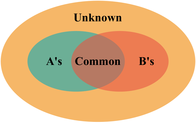
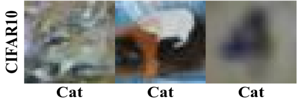
Figure 1: An overview of the feature space and overconfidence examples of discriminator models.

Out-of-distribution (OOD) detection is a crucial task for deep learning models, as it helps them determine their capability boundary and prevents them from being deceived by OOD data. This task is closely related to many real-world machine learning applications, such as cybersecurity [1], medical diagnosis [2, 3], and autopilot [4]. Existing methods for OOD detection can be broadly categorized into discriminator-based and generation-based approaches. Discriminator-based methods [5] utilize either the logit or feature space to perform detection, while generation-based methods [6, 7] rely on reconstruction differences in data space or density estimation in latent space.

Discriminator-based methods are generally faster and more effective in extracting useful features for OOD detection. However, Nguyen et al. [8] show that some OOD data can be misclassified with high confidence, resulting in the overconfidence problem. On the other hand, generation-based methods can capture the entire distribution

but often lack effective indicator scores to compete with state-of-the-art discriminator-based methods.

In this paper, we propose a novel approach that combines discriminator and generation models to counteract each other’s limitations. Our analysis reveals that discriminator models do not assign significant importance to common features of different categories, which may be important for OOD detection. The relationship between common and exclusive features is depicted in Figure 1. Thus, we introduce a new assumption that discriminator models focus on specific features of the input, leading to the overconfidence problem. For example, the model focuses on certain patterns in Figure 1 and 2, both misclassifying OOD data with high confidence. Conversely, generation models can capture the entire data distribution, including the common features of different categories. Therefore, we use them to enhance the input and help the discriminator models. This approach is analogous to the principle behind smoke alarms. Because the air is flowing, we can install a fixed smoke alarm to monitor the whole house, while generation models make information “flow” more effectively.

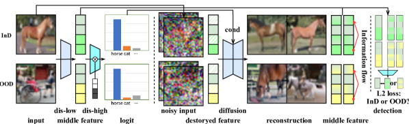
Figure 2: The pipeline of our OOD detection method. The discriminator model can identify more information through the flow of information during the diffusion denoising process. Here, We use a mask to represent the information loss in the discriminator model.

To develop effective generation strategies, we incorporate diffusion models (DMs) into OOD detection. DMs have achieved state-of-the-art results in many generation tasks, including Vahdat et al. [9] and Ho et al. [10]. We observe that the diffusion denoising process (DDP) of DMs serves as a novel form of asymmetric interpolation, functioning as both a reconstruction and interpolation process. The reconstruction property enables DDP to enhance the input and enable it to “flow’, while the interpolation property helps to maintain control over the adjustments. Our method employs a two-step framework for OOD detection. First, we utilize DDP to generate additional samples based on the input. Next, we input all of these samples into a pre-trained discriminator model. Anomalies previously ignored by the discriminator model are exposed in the flow of information formed by DDP, and then the feature results of the discriminator model change sharply. Therefore, we utilize the norm of the dynamic change in features as the indicator score. The pipeline is illustrated in Figure 2.

We choose six representative methods to compare with our methods on CIFAR10, CIFAR100, and ImageNet. According to our experiments, our methods outperform existing methods. Notably, for the challenging InD ImageNet and OOD species datasets, our method achieves an AUROC of 85.7, surpassing the previous SOTA method’s score of 77.4. Our work has the following contributions:

• We propose a new perceptron bias assumption that explains the overconfidence problem, suggesting that discriminator models are more sensitive to certain features of the input.

• We introduce diffusion models into OOD detection and demonstrate that the diffusion denoising process of invertible DMs serves as a novel form of asymmetric interpolation, enabling effective enhancement of input data while maintaining control in the denoising process.

• We design a two-step detection method that utilizes a ResNet to extract features and the diffusion denoising process to mitigate overconfidence issues. Our method is highly explicable and achieves state-of-the-art results.

2 Background

In this section, we first introduce existing methods for OOD detection. Then, we show the development of diffusion models related to our paper. Due to the limited space in the main paper, more related works about diffusion models and similarities and differences between our method and existing methods can be found in Appendix A.1.

2.1 Out-of-distribution Detection

OOD detection is an important task that can help neural networks to determine their capability boundary. More specifically, let $X=\{x_{1},\dots,x_{n}\}\sim p$ be a group of images from the in-distribution (InD) $p$. We want to build a detector $f$ that $f(x_{1},\dots,x_{n})=1,\forall i,p(x_{i})\geq\sigma$ and $f(x_{1},\dots,x_{n})=0,\forall i,p(x_{i})\leq\sigma$. Here, $\sigma$ controls the decision boundary. When we get another group of data $Y=\{y_{1},\dots,y_{n}\}$, we decide whether this group is from InD $p$ or an unknown distribution $q$ based on the results of $f$. If $n=1$, this is pointwise OOD detection, and if $n\geq 2$, this is group OOD detection. In general, the existing OOD detection methods can be categorized into discriminator-based and generation-based methods.

Discriminator-based methods design indicator scores based on the output of discriminator models. Some methods can be used without modifying the model. ODIN [11] uses temperature scaling and the softmax results to detect OOD samples. ViM [5] combines the information of features and logits. KNN [12] includes the kth nearest neighbor of the input in feature space into the detection process. Some methods try to improve the detection ability in the training process. G-ODIN [13] designs a new loss function. ConfGAN [14] generates OOD data using GANs to help the discriminator models to determine the boundary. PixMix [15] uses data augmentation to improve the detection results. SSD [16] uses self-supervised learning to improve feature extraction.

Generation-based methods employ the difference in reconstruction between the input space or the density estimation in the latent space for OOD detection. The former assumes that the generation models can reconstruct the in-distribution data more effectively, while the latter utilizes the distribution transformation capability of generation models to convert the input distribution into a simple Gaussian distribution. In more detail, the likelihood of the input is a direct indicator score, but Nalisnick et al. [17] find that OOD data can also locate in the high-likelihood area. Nalisnick et al. [7] find the InD data is concentrated in the typical set instead of the high likelihood area and design new methods using the typical set. Serrà et al. [18] find that we can use input complexity to correct the bias of likelihood. In addition to the likelihood, many existing statistical methods can detect whether a distribution obeys standard Gaussian distribution. Zhang et al. [19] uses KL-divergence to detect OOD data. Jiang et al. [20] use a nonparametric statistics method, the Kolmogorov-Smirnov test.

2.2 Diffusion Model

Classical diffusion model

DMs build a transformation from Gaussian distribution to image distribution through a multistep denoising process. Given a data distribution $x_{0}\sim q(x_{0})$, the diffusion process satisfies a Markov process as following [21]:

$$\begin{split}&q(x_{1:T}|x_{0})=\prod_{t=1}^{T}\mathcal{N}(\sqrt{1-\beta_{t}}x_{t-1},\beta_{t}I)\\ &q(x_{t}|x_{0})=\mathcal{N}(\sqrt{\bar{\alpha}_{t}}x_{0},(1-\bar{\alpha}_{t})I).\end{split}$$ (1)

Here, $T=1000$, which is the max iteration step. $\beta_{t}\in(0,1)$, which controls the speed of adding noise. Additionally, $\alpha_{t}=1-\beta_{t}$, $\bar{\alpha}_{t}=\prod_{i=1}^{t}\alpha_{i}$, $\bar{\mu}_{t}=\frac{\sqrt{\bar{\alpha}_{t-1}}\beta_{t}}{1-\bar{\alpha}_{t}}x_{0}+\frac{\sqrt{\alpha_{t}}(1-\bar{\alpha}_{t-1})}{1-\bar{\alpha}_{t}}x_{t}$ and $\bar{\beta}_{t}=\frac{1-\bar{\alpha}_{t-1}}{1-\bar{\alpha}_{t}}\beta_{t}$. The objective function is defined by:

$$\small\begin{split}L_{t}=\mathbb{E}_{x_{0},\epsilon}\left[\frac{\beta_{t}^{2}}{\alpha_{t}(1-\bar{\alpha}_{t})}||\epsilon-\epsilon_{\theta}(\sqrt{\bar{\alpha}_{t}}x_{0}+\sqrt{1-\bar{\alpha}_{t}}\epsilon,t)||^{2}\right].\end{split}$$ (2)

Here, $\epsilon_{\theta}$ is an estimate of the noise $\epsilon$. After we get well-trained $\epsilon_{\theta}$, according to Song et al. [22], the denoising process of Denoising Diffusion Probabilistic Models (DDPMs) and Denoising Diffusion Implicit Models (DDIMs) satisfies:

$$x_{t-\delta}=\sqrt{\bar{\alpha}_{t-\delta}}\left(\frac{x_{t}-\sqrt{1-\bar{\alpha}_{t}}\epsilon_{\theta}(x_{t},t)}{\sqrt{\bar{\alpha}_{t}}}\right)+\sqrt{1-\bar{\alpha}_{t-\delta}-\sigma^{2}_{t}}\epsilon_{\theta}(x_{t},t)+\sigma_{t}\epsilon_{t}.$$ (3)

Here, $\delta$ is the iteration step size. If $\sigma_{t}$ equals one, Equation (3) represents the denoising process of DDPMs; if $\sigma_{t}$ equals zero, this equation represents the denoising process of DDIMs. In Appendix A.2, we will further describe how to make the iteration of the diffusion model fast and invertible.

Classifier-free guidance Ho and Salimans [23] show a simple and effective way to generate conditional samples called classifier-free guidance. It adds a condition embedding $c$ into the model during the training process and changes the estimation of noise as:

$$\bar{\epsilon}_{\theta}(x_{t},c,t)=\epsilon_{\theta}(x_{t},\emptyset,t)+\omega\left(\epsilon_{\theta}(x_{t},c,t)-\epsilon_{\theta}(x_{t},\emptyset,t)\right).$$ (4)

Here, $\omega$ is the guidance weight, which controls the balance between realness and diversity.

3 Perceptron Bias and Diffusion Denoising Process

In this section, we propose a new perceptron bias assumption to explain the overconfidence of discriminator models and highlight the potential of generation models to address this issue. We then use a toy example to demonstrate how generation models can be used to reduce information loss and incorporate the diffusion denoising process (DDP) into OOD detection. We show that DDP serves as both a reconstruction and interpolation operator, making it well-suited to address the perceptron bias problem. We then visualize the impact of DDP on real-world scenarios and explain how to select indicator scores. Furthermore, we introduce conditional diffusion models to address multiclass detection and provide our algorithms.

3.1 Why Generation Models are Essential?

In the introduction, we briefly introduce the perceptron bias problem in discriminator models. Here, we provide a more detailed analysis of this issue. We find discriminator models are more sensitive to features that belong exclusively to certain categories and do not place as much value on common features. This is a reasonable decision for an “smart” discriminator model due to both the model structure and the training process.

In terms of the model structure, they employ convolutional and pooling layers to compress the data space. Consequently, the models must learn to eliminate some relatively useless information to achieve high classification accuracy. In terms of the training process, some features may not be crucial for the original classification problem. For instance, the eyes may not be a significant feature for distinguishing between dogs and cats. Consequently, the models may ignore this information. However, this feature is crucial in determining whether the input is animal or OOD data and should not be disregarded. In summary, the perceptron bias problem can be described as follows:

Definition 3.1.

The perceptron bias problem is that a fixed discriminator model focuses only on certain features of the input.

These analyses highlight that a discriminator model is not omniscient and suffers from excessive information loss, particularly common features that belong to different categories. In contrast, generation models can effectively model information, including common features. This underscores the potential of generation models to enhance OOD detection.

3.2 Toy Example

To better illustrate the potential of generation models in addressing this issue, we simplify the perceptron bias to a constraint operator $f|_{S}$, with the core idea of binarizing such bias into pass or fail. The data passes through a discriminator model as if it had been filtered through a mask, resulting in the loss of some information.

Here, the input space is a 2-dimensional square space. The support area $S$ of the restriction operator $f$ is a collection of small patches $\bigcup_{i\in I_{S}}S_{i}$ at the pixel level. Our InD data is a uniform distribution in a spherical neighborhood of zero (the empty image), and our objective is to detect whether a new input is within the neighborhood of zero. We illustrate this toy example in Figure 4, where the top row shows two normal cases and one bad case under this setting. The bad case appears to be zero after the restriction operator $f$. In the middle row of Figure 4, we correct the result by using three additional operators: moving, mixing, and reconstruction.

The first two methods can perfectly solve the information loss problem in Figure 4, and the proof is provided in Appendix A.3. The key idea behind these methods is to move or mix information from one place to another. This allows the detector $f$ to obtain the complete information from a small support area $S$, thereby reducing the information loss. Moreover, these methods can be extended to support areas $S$ of any shape, as demonstrated in the right side of the bottom row of Figure 4. Therefore, we can design general operators for different $S$, which is essential as we cannot always obtain the exact $S$ in real-world scenarios.

Although the above two methods exemplify our primary concept, their capacity is restricted to the pixel level. To design a more general method, we propose a third reconstruction operator that first destroys images and then employs a generation model to reconstruct them, which is also a form of data augmentation. While we refer to it as reconstruction, it does not restore the input entirely but rather reconstructs the missing parts based on available input information. This creates a form of information “flow” from one place to another, such as moving (e.g., the cat’s face moving to the left and down), mixing (e.g., the boundary of each small box becoming unclear), and semantic-level moving (e.g., the cat’s color becoming lighter), as shown in Figure 4.

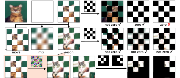
Figure 3: A toy OOD detection process to detect whether the input is a neighbor of zero (the empty image). The top row shows two normal cases and a bad case. The middle row provides three different additional operators to correct this bad case. The bottom row shows that the above operators are suitable for different shapes of support areas.

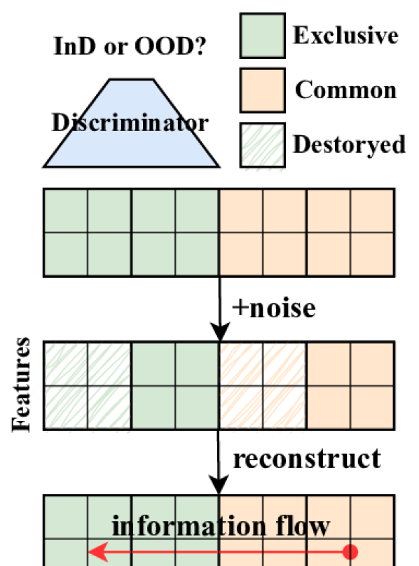
Figure 4: Common features flow towards the exclusive area and then can be detected by the discriminator model.

Core Concept In essence, the interplay between discriminator and generation models can be likened to that of smoke alarms and the flow of air. While a smoke alarm is stationary within a building, it is capable of monitoring the entire space due to the movement of air. Similarly, although the discriminator may focus on specific features, the generation models can facilitate the flow of information to enable effective OOD detection. We illustrate this process in Figure 4.

3.3 Why Choose Diffusion Models?

While all generation models have the potential to reconstruct damaged images, this strategy also has its weaknesses. As shown in Figure 4, we can detect OOD examples more accurately using a reconstruction operator. However, we also need to ensure that pure white pictures remain clean. This challenge highlights the need for more control over the reconstruction strategy. We find that diffusion models are particularly suitable for two main reasons.

Controlled noise intensity The first advantage of diffusion models is their ability to naturally control the intensity of the added noise, which in turn affects the reconstruction results. This is important because combining different intensities of noise would make the reconstruction much more complicated and challenging to design indicators for OOD detection.

Controlled flow vector The flow vector is the difference between the original input and the reconstruction output. We find that the diffusion denoising process (DDP) of diffusion models is a form of interpolation under invertible conditions. As such, it serves as both a reconstruction and interpolation operator. The fact that DDP is a reconstruction operator implies that it can preserve InD data relatively unchanged while moving OOD data towards the high-density area of InD, which demonstrates the control of the norm of the flow vector. The fact that DDP is an interpolation operator suggests that we can control the direction of change and maintain InD data changes within the InD area when timestep $t$ is large, which demonstrates the control of the direction of the flow vector. By combining norm and direction control, we can control the flow vector.

Many previous papers use diffusion models to interpolate two inputs, but our method is different from the existing symmetric approach using spherical linear interpolation [24]. We combine invertible diffusion models and DDP $\Phi$ to obtain a new asymmetric interpolation. The algorithm is shown in Algorithm 1. Here, $\Phi(x,t_{1},t_{2})$ refers to the DDP process from $t_{1}$ to $t_{2}$. Setting $x_{1}$, $x_{2}$ are two images and $\epsilon_{2}=\Phi(x_{2},0,T)$ is the reverse noise of an image $x_{2}$, we use $x_{1}$ and $\epsilon_{2}$ to obtain $x_{t}^{\text{inter}}$, then denoise it to obtain the interpolation result $x^{\text{inter}}$. When $t$ equals zeros, we do not add any noise, and $x^{\text{inter}}_{0}=x_{1}$, so the interpolation result is $x_{1}$. When $t$ equals $T$, we remove the total image $x_{1}$ and only leave $x^{\text{inter}}_{T}=\epsilon_{2}$, we will perform a full denoising process to this noise $\epsilon_{2}$. Because the denoising process is invertible, we can get the image $\Phi(\epsilon_{2},T,0)=x_{2}$. Therefore, the outputs of DDP gradually change from $x_{1}$ to $x_{2}$. Figure 5 shows the three different interpolation results. The first row uses the cat as $x_{1}$, and the second row uses the car as $x_{1}$. We can find that $x_{1}$ can be better preserved compared to the symmetric interpolation in the third row. In summary, we have:

Proposition 3.2.

The invertible diffusion-denoising process is an asymmetric interpolation.

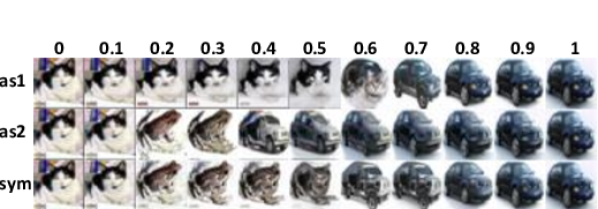
Figure 5: Interpolation results using two fixed images.

Algorithm 1 Asymmetric interpolation

1:input: Images $x_{1},x_{2}$, interpolation timestep $t$

2:$\epsilon_{2}=\Phi(x_{2},0,T)$

3:$x_{t}^{\text{inter}}=\sqrt{\bar{\alpha}_{t}}x_{1}+\sqrt{1-\bar{\alpha}_{t}}\epsilon_{2}$

4:$x^{\text{inter}}=\Phi(x_{t}^{\text{inter}},t,0)$

5:return $x^{\text{inter}}$

3.4 Diffusion-based Out-of-distribution Detection

In the above, we show the advantages of DDP using a toy example and theoretical analysis. Here, we show the effect of DDP in a more complex example and design proper indicator scores. Specifically, we consider the last convolutional layer of a multi-layer model. In this setting, the input of this layer has many channels. To be more precise, the input is in $\mathbb{R}^{m\times m\times c}$ and is a combination of $c$ elements in the feature space $\mathbb{R}^{m\times m}$. As a result, a single input becomes $c$ points in the feature space instead of a single point.

In Figure 6, we abstract the feature space into 2-dimensional space, and the ideal feature space related to the target class is the light blue square. The points in the feature space represent $c=6$ features of a single input, and the corresponding arrow shows the information flow of these features under DDP. We use the dark blue area to show the features used by the convolutional kernels of the last convolutional layer. The output of each convolutional kernel is a single value, the number of points $N$ that fall in its sensitive area. Then, we sum them to get the final result. This example is a simplification of the process used to compute confidence.

For a normal InD input (the top row), DDP changes the image but still maintains it in the InD area. Its corresponding feature points move within the class-related feature area (light blue area). The number of feature points that can be captured by the discriminator (dark blue area) maintains a dynamic balance. For a normal OOD input (the middle row), the image contains no class-related features. Its feature points fall outside the class-related feature area. DDP pulls the OOD input to the high-density area of the training data. For example, a banana becomes a yellow plane, and the number one becomes a white cat. The number $N$ of the captured feature points increases at the same time. For more challenging OOD data (the bottom row), it is not InD, but it contains some class-related features. For example, a furry toy and the number four are incorrectly identified as cats. Its class-related features are relatively sparse but happen to be captured by the discriminator (dark blue area) by coincidence or man-made. However, the imbalance distribution of points in the dark blue area and the remaining causes more points to go out than come in under DDP, which causes a rapid decline of $N$. Therefore, all two kinds of OOD input can be detected by the change of confidence. Our main advantage is that we detect the balance between the features of interest to the discriminator and the remaining class-related features. This balance ensures that we can indirectly understand the whole feature space by detecting only the features of interest to the discriminator. More analysis and results about the effect of DDP are in Appendix A.4.

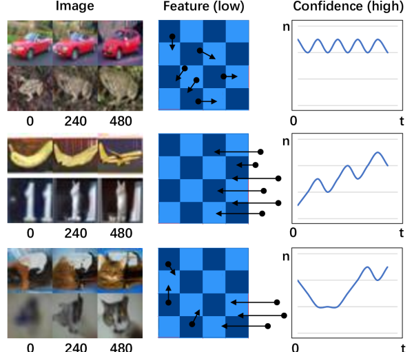
Figure 6: The change in image space and different feature spaces under the disturbance of DDP.

Algorithm 2 Conditional Reconstruction

1:Input: Image $x$, timestep $t$

2:$y=\text{FC}(\text{ResNet}(x))$

3:$\epsilon\sim\mathcal{N}(0,1)$

4:$x_{\text{noise}}=\sqrt{\bar{\alpha}_{t}}x+\sqrt{1-\bar{\alpha}_{t}}\epsilon$

5:$x_{\text{recon}}=\Phi(x_{\text{noise}},y,t,0)$

6:return $x_{\text{recon}}$

Algorithm 3 OOD detection

1:Input: Image $x$, additional samples $x_{\text{recon}}$

2:fea = ResNet($x$)

3:$\text{fea}_{\text{recon}}=\text{ResNet}(x_{\text{recon}})$

4:score = $\sum|\text{fea}-\text{fea}_{\text{recon}}|$

5:if $\text{score}>\delta$ then

6:     return OOD

7:end if

Multiclass Detection In real cases, it is often necessary to consider multiple categories. One key change is that the output is the probability of multiple categories, which is a multi-value vector. As a result, we need to modify our object of detection from the change of single-value confidence to a multi-value vector. This inspires us that the form of output is not limited, and we can also detect changes in any intermediate feature space as our indicator score.

The second change is that we need to not only keep the inputs within the InD area but also prevent category migration for InD inputs. In this case, we require the interpolation property, and there are two options available. Firstly, we can search for the nearest neighbor of the input in the image space and generate corresponding noises. We can then interpolate these noises with the original input using DDP. Another more intriguing option is to train a conditional diffusion model and fix the class condition to the class of the input. Then, all noise corresponds to images in the target class. Instead of searching for noise first, we can interpolate the input with any noise now.

In summary, our method uses conditional and invertible DDP to facilitate the flow of information and uses a discriminator model to generate the features. We then determine the OOD samples based on the dynamic change in the feature spaces. Our algorithms are in Algorithm 2 and 3.

4 Experiment

4.1 Setup

We evaluate our methods on OpenOOD benchmarks [25], using CIFAR10, CIFAR100, and ImageNet as InD datasets. For CIFAR10, we use CIFAR100, TinyImagenet [26], SVHN [27], Texture [28] and Places365 [29] as OOD datasets. For CIFAR100, the OOD datasets are the same, except for swapping CIFAR100 for CIFAR10 as the OOD dataset. For ImageNet, we use Species [30], iNaturalist [31], Texture, Places365, and SUN [32] as OOD datasets. To ensure that there is no overlap between the InD and OOD datasets, all OOD datasets are meticulously filtered.

For a fair comparison, we first train discriminator and generation models using the training set. We evaluate the results by calculating FPR@95 and AUROC [33] between the test set of the InD dataset and others, which avoids the influence of model overfitting. All images from different datasets are resized into $32\times 32$ for CIFAR10/100 and $224\times 224$ for ImageNet. For CIFAR10/100, we utilize a pre-trained ResNet18 [34] and the diffusion model from DDPM, trained by ourselves. For ImageNet, we use a pre-trained ResNet50 and a pre-trained latent diffusion model [35]. More detailed settings and hyperparameters of our method can be found in Appendix A.5.

Table 1: The AUROC results of different methods on CIFAR10 and CIFAR100. The higher results are better and the bold results are the best in each case.

InD	cifar10					cifar100
OOD	cifar100	tin	svhn	texture	place	cifar10	tin	svhn	texture	place
ODIN	77.76	79.65	73.41	80.76	82.61	78.1	81.33	70.97	79.31	79.76
EBO	86.19	88.61	88.42	86.88	89.62	79.07	82.46	77.81	77.84	80.16
ReAct	86.37	88.91	89.52	88.19	90.1	73.48	79.63	84.45	83.58	76.94
MLS	86.14	88.53	88.47	86.89	89.5	79.18	82.59	77.68	77.94	80.29
VIM	87.19	88.86	97.28	96.03	90.03	71.54	78.34	81.15	87.41	75.77
KNN	89.62	91.48	95.07	92.84	91.86	76.48	83.33	82.09	83.69	79.03
Diff(ours)	90.53	92.85	95.09	93.66	92.65	76.43	84.23	84.96	80.64	78.7

Table 2: The AUROC results of different methods on ImageNet and the mean and standard deviation of the results on CIFAR10, CIFAR100, and ImageNet. A higher mean value is better, while a lower standard variance is better. The best results are in bold.

InD	imagenet					cifar10		cifar100		imagenet
OOD/stat	specie	inatur	texture	place	sun	mean	std	mean	std	mean	std
ODIN	71.51	91.15	87.5	84.5	86.9	78.8	3.14	77.9	3.61	84.3	6.75
EBO	71.98	90.63	86.73	83.97	86.58	87.9	1.24	79.5	1.73	84.0	6.36
ReAct	77.43	96.4	90.49	91.92	94.4	88.6	1.29	79.6	4.10	90.1	6.67
MLS	72.89	91.15	86.41	84.19	86.6	87.9	1.22	79.5	1.79	84.2	6.11
VIM	69.43	86.4	97.35	76.99	79.62	91.9	4.02	78.8	5.32	82.0	9.42
KNN	66.84	84.16	96.02	70.22	76.65	92.2	1.79	80.9	2.76	78.8	10.5
Diff(ours)	85.03	97.05	94.76	88.86	92.99	93.0	1.49	81.0	3.24	91.7	4.29

4.2 Out-of-distribution Detection

In Table 1, we choose six representative baselines, which do not adjust the discriminator model similar to our method. ODIN [11] uses temperature scaling and gradient-based input perturbation. EBO [36] uses an energy-based function. ReAct [37] uses rectified activation. MLS [30] uses maximum logit scores. VIM [5] combines the information of feature space and logic space. KNN [12] uses the nearest neighbor in the feature space. Our method surpasses all these methods in five out of ten cases and achieves comparable results in the remaining cases. In Table 2, we find that our method performs better than the other methods in two out of five cases and achieves comparable results in the remaining cases. This shows the effectiveness of our method on datasets of varying sizes. Moreover, our method has low standard variance across different OOD datasets, indicating its excellent generalization ability. FPR@95 results can be found in Appendix A.6.

Table 3: The AUROC results when we treat misclassified data in CIFAR100 as a kind of OOD data.

OOD	wrong	cifar10	tin	svhn	texture	place
MLS	83.93	86.50	89.30	85.16	85.49	87.55
VIM	79.31	78.03	84.26	87.00	91.19	81.96
KNN	84.36	83.59	89.88	88.98	89.75	86.19
Diff	84.96	85.67	91.87	96.50	89.56	88.27

OOD detection is widely used in scenarios with high-security requirements. It is also imperative to identify any misclassified data from the InD dataset. Thus, we treat the misclassified data of the pre-trained ResNet18 as a new form of OOD data. ResNet18 has an accuracy of only 78% on CIFAR100, making it an appropriate candidate for demonstrating the impact of misclassified data. Our method achieves SOTA results in distinguishing between correctly and incorrectly classified data in the training datasets. Under this setting, MLS and VIM outperform us on only one OOD dataset, respectively, and the gap is small. On all other datasets, our method is substantially ahead of all other methods. By comparing the results in the corresponding positions in Table 1 and 3, we find that after removing the misclassified data from InD, the OOD detection results of all methods are improved, with our method having the biggest improvement. This means that all methods tend to treat misclassified data as OOD data. The detection results of misclassified data and classical OOD data are mixed, which limits the classical OOD detection results.

4.3 Ablation Study

Here, we show the influence of each item and hyperparameter in our method. Here, the AUROC results are the average of five AUROC results using all OOD datasets on CIFAR10. More ablation study results can be found in Appendix A.7.

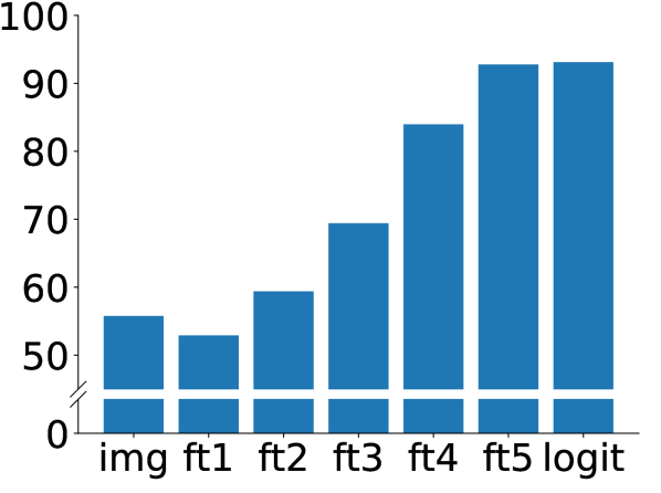
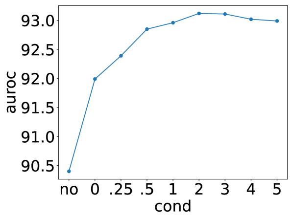
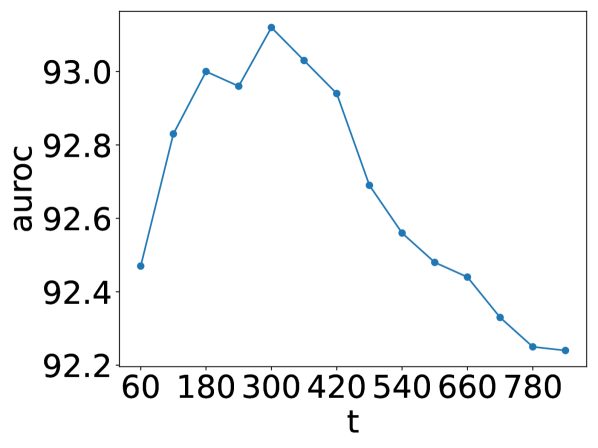
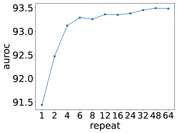
Figure 7: the AUROC results obtained under different detection spaces, guidance weights, disturbance degrees, and resampling sizes on CIFAR10.

Detection space In Figure 7.1, we compare the results obtained when using different detection spaces, including the input image space, different level feature spaces, and the logit space. We achieve the best results when using the high-level feature or the logit. The low-level features and image space yield relatively poor results, primarily due to the redundancy of information at these levels. This highlights the importance of the discriminator model to the generative model in OOD detection. We also observe that setting a threshold for the final feature space can improve detection results, similar to ReAct [37].

Condition In Figure 7.2, we examine the impact of different guidance weights $\omega$ on conditional diffusion models. We find that higher guidance weights result in relatively better outcomes, indicating that realness is more critical than diversity in the OOD detection task. Furthermore, we find that the conditional version outperforms the unconditional version, with the detection results showing a more significant improvement on CIFAR100. This suggests that conditional control is essential, and higher guidance weights $\omega$ are required for more classes.

Timestep In Figure 7.3, we investigate how to select the optimal value of $t$ in DDP. We find that the best choice is $t=300$ for small datasets. When $t\leq 300$, the difference caused by DDP is still not distinct enough. When $t\geq 300$, the noise item accounts for a larger and larger proportion, causing information loss and limiting the OOD detection results. For large datasets, the information in images is redundant, necessitating more noise to create a noticeable change. The best $t$ is 600 in this case.

Resampling In Figure 7.4, we determine the influence of the repeated sampling size. According to our analysis, the consistent detection results are maintained by dynamic balance. Therefore, we need to resample several times to eliminate the random error in DDP. We observe that a larger number of resampling leads to better results, and four times resampling is sufficient.

5 Conclusion

In this paper, we start with the analysis that discriminator models may ignore common features which are important for OOD detection. Based on that, we provide a new perceptron bias assumption to explain the overconfidence problem. Under this assumption, we first show the potential of generation models and develop the diffusion denoising process of diffusion models as the solution. Then, we demonstrate how to design indicator scores in real-world scenarios and how to apply our method to multi-class situations. Our approach is highly interpretable and employs simple training objectives, including softmax loss for discriminator models and L2 loss for diffusion models. Using the combination of a ResNet and a diffusion model, we get SOTA results on CIFAR10, CIFAR100, and ImageNet. We believe that our strategy can benefit the OOD detection community and has the potential to be applied to OOD generalization and other related tasks.

While the limitations of our method include the detection speed and the training cost of diffusion models, the advancements in effective training and sampling for diffusion models are rapidly progressing. For instance, consistency models [38] can complete sampling in several steps, and ControlNet [39] can improve training efficiency. We aim to leverage these new developments to enhance the efficiency of our method in the future.

Appendix A Supplementary Material

A.1 Related Work

Here, we introduce more related works to show the recent development of diffusion models. Then we show similarities and differences between our method and existing works to emphasize our advantages.

A.1.1 Diffusion Model

Denoising Diffusion Probabilistic Models (DDPMs) [21] successfully generate high-quality images and make DMs become popular. For now, DMs can not only generate unconditional high-quality images but also are applied to many different fields. For the conditional generation task, DMs can do interpolation, manipulation, image-editing, style transformation and text-conditional generation [40, 41]. For different data types, DMs can do text [42], audio [43, 44] and video generation.

The main challenge for DMs is that they require hundreds to thousands of iterations to produce high-quality results, which limits the application of DMs. After DDPMs, many works try to make DMs faster and better. Some of them focus on the denoising equations of DMs. Nichol and Dhariwal [45] design a better time schedule for the denoising process. Liu et al. [46] provide new numerical methods for the denoising process. Bao et al. [47] find analytic results for the variance of the denoising process. Some of them try to design new training strategies and new models. Salimans and Ho [48] use distillation to accelerate DMs. Dhariwal and Nichol [49] change the model structure from Unet to GAN to make each iteration step more powerful. What’s more, Song et al. [50] first shows that DMs can be rewritten as two neural differential equations [51, 52]. Therefore, the numerical methods used to accelerate neural differential equations can also be used here.

A.1.2 Similarity and difference

Several baselines are similar to our method in some ways. The first one is KNN [12], which does a KNN search in the feature space. However, KNN ignores the possibility that an OOD input may have a similar feature as InD data. All methods that only use the final feature have this problem. They can not solve the information loss of discriminator models. In addition, using KNN in the input space directly is also invalid, because of data sparsity and irrelevant information interference. Our method uses ResNet to extract useful information and uses diffusion models to solve the information loss at the same time.

Another similar approach is data generation. Existing methods use generation models to generate OOD data [53, 54, 55, 56] to help the discriminator models to know the capability boundary. This requires careful design of additional loss functions and the whole pipeline. Our method uses classical loss functions and training processes for both discriminator and generation models. Then our method uses the generation models to do interpolation between the new input data and the training data and puts all results into the discriminator model.

Data augmentation is also similar to our method. Some of them use augmentation results to retrain discriminator models, but our generation and discriminator models are trained separately. Although these methods can enhance the richness of data and keep the data realistic, some new methods start to add complex and unreal augmentation [15], which increases the burden on the models and lacks clear motivation. Some of them only use augmentation results in the detection processes. However, existing methods focus on the denoising process, which is a trade-off between remaining InD data unchanged and enhancing the input, which becomes an obvious bottleneck. We find that keeping InD related unchanged is unnecessary. Our method replaces the denoising operator with an interpolation operator. The interpolation operator only remains the InD input in the InD area, which is good enough for OOD detection and provides more possibilities to enhance the input.

A.2 Invertible Diffusion Model

Here, we introduce more details of the invertible diffusion model used in this paper. Then, we analyze how to make the iteration of diffusion models more invertible in practice. After that, we introduce asymmetric and symmetric interpolations under the invertible condition.

A.2.1 Method detail

Score-based generation model

Song et al. [50] show that the diffusion-denoising process can also be treated as two differential equations:

$$\begin{split}dx&=(\sqrt{1-\beta(t)-1})x(t)dt+\sqrt{\beta(t)}dw\\ dx&=\left((\sqrt{1-\beta(t)-1})x(t)-\frac{1}{2}\beta(t)s_{\theta}(x(t),t)\right)dt.\end{split}$$ (5)

This is called probability flows (PFs). The noise $\epsilon_{\theta}$ of DMs and the gradient of logic likelihood $s_{\theta}$ are equivalent [47]. More specifically, we have that $s_{\theta}(x,t)=-\frac{1}{1-\bar{\alpha}_{t}}\epsilon_{\theta}(x,t)$.

Pseudo numerical method

Liu et al. [46] provide pseudo numerical methods for diffusion models (PNDMs) to accelerate DDIMs. PNDMs define Equation (3) with $\sigma_{t}=0$ as transfer function:

$$\phi(x_{t},\epsilon_{t},t,t-\delta)=\frac{\sqrt{\bar{\alpha}_{t-\delta}}}{\sqrt{\bar{\alpha}_{t}}}x_{t}-\frac{(\bar{\alpha}_{t-\delta}-\bar{\alpha}_{t})}{\sqrt{\bar{\alpha}_{t}}(\sqrt{(1-\bar{\alpha}_{t-\delta})\bar{\alpha}_{t}}+\sqrt{(1-\bar{\alpha}_{t})\bar{\alpha}_{t-\delta}})}\epsilon_{t}.$$ (6)

PNDMs combine this transfer function with the noise estimated by classical numerical methods, like the linear multistep method, to get the new denoising equations:

$$\begin{cases}&\epsilon_{t}^{\prime}=\frac{1}{24}(55\epsilon_{t}-59\epsilon_{t+\delta}+37\epsilon_{t+2\delta}-9\epsilon_{t+3\delta})\\ &x_{t-\delta}=\phi(x_{t},\epsilon_{t}^{\prime},t,t-\delta).\end{cases}$$ (7)

Here, $\epsilon_{t}=\epsilon_{\theta}(x_{t},t)$. Both PFs and PNDMs accelerate the denoising process without loss of quality.

A.2.2 Invertibility

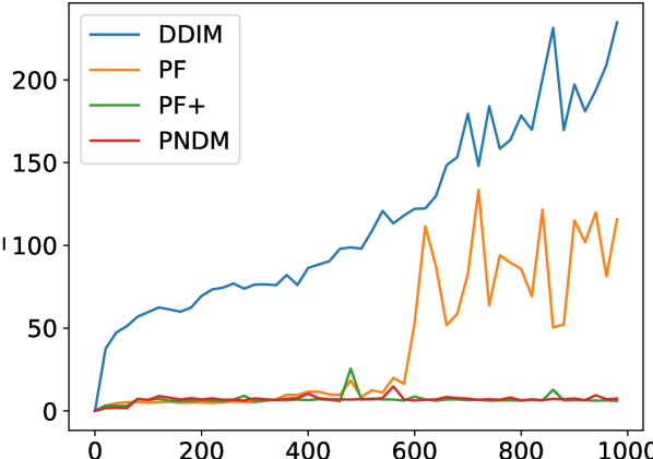
Figure 8: The reconstruction error under different iteration interval $[0,t]$ and fixed step size 20.

We show the test results in Figure 8. For DDIMs, the error occurs at the beginning, and the error accumulates with the increase of the total generation step. For PFs, the initial error is not huge, but the cumulative error occurs when the number of the total generation steps is bigger than 500. DDIMs are first-order methods, and other methods are high-order methods. We can say higher convergent order can increase the invertibility. PFs use numerical methods of adaptive step size, and PNDMs use methods of fixed step size. Therefore, we think that fixed step size can also benefit invertibility. To verify this, we replace the methods of adaptive step size used by PFs with the methods of fixed step size and call it probability flows plus (PFs+). We find that the errors decrease immediately. The reason is that fixed step size maintains consistency between the sampling locations of the forward and reverse processes, which benefits the invertibility. Combining the above analysis, we have the following property:

Proposition A.1.

High convergent order and fixed iteration step size can improve the invertibility of DMs under fixed total iteration steps.

A.2.3 Interpolation

In Algorithm 4 and 5, we introduce two types of interpolation using diffusion models. The positions of $x_{1}$ and $x_{2}$ are symmetric in the original interpolation and asymmetric for the asymmetric one. According to our experiment, $x_{1}$ is more important in asymmetric interpolation. The visualization of these interpolations can be found in Fig 9.

Because the $x_{1}$ can be preserved at the beginning, which is more like a denoising operator. When the interpolation ratio becomes bigger, the results change from $x_{1}$ to $x_{2}$ smoothly, which is more like an interpolation operator. Therefore, DDP is a combination of denoising and interpolation operators and the timestep $t$ controls the ratio of denoising and interpolation.

Algorithm 4 Symmetric interpolation

1:Input: Images $x^{1},x^{2}$, generation gap $\delta$, interpolation rate $\sigma$

2:$x_{T}^{1},x_{T}^{2}=\Phi(x^{1},0,T,\delta),\Phi(x^{2},0,T,\delta)$

3:$x_{T}^{\text{inter}}=\text{Slerp}(x_{T}^{1},x_{T}^{2},\sigma)$

4:$x^{\text{inter}}=\Phi(x_{T}^{\text{inter}},T,0,\delta)$

5:

6:return $x^{\text{inter}}$

Algorithm 5 Asymmetric interpolation

1:Input: Images $x^{1},x^{2}$, generation gap $\delta$, interpolation timestep $t$

2:$x_{T}^{2}=\Phi(x^{2},0,T,\delta)$

3:$x_{t}^{\text{inter}}=\sqrt{\bar{\alpha}_{t}}x^{1}+\sqrt{1-\bar{\alpha}_{t}}x_{T}^{2}$

4:$x^{\text{inter}}=\Phi(x_{t}^{\text{inter}},t,0,\delta)$

5:

6:return $x^{\text{inter}}$

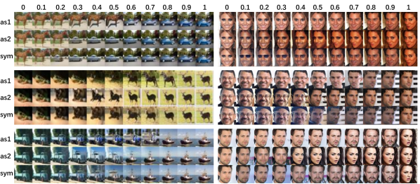
Figure 9: The results of asymmetric and symmetric interpolations using two fixed images from CIFAR10 or CelebA.

A.3 Proof of toy example

Here, we prove that the moving and mixing operators can perfectly solve the toy example. To make this claim strict, we need to make some definitions.

We first transfer OOD detection and the design of our two-step method into a formal problem. Following the definitions in Section 2.1, the detector is a function $f:U\to\mathbb{R}$ that can be an analytic function or a neural network defined on a certain space $U$. The detection problem is that given a distribution $p$ on $U$, let $W\triangleq\{x\in U|p(x)>\sigma\}$ and we want to find a detector $f$ that satisfies $f^{-1}(1)=W$ exactly. The two-step method starts with a relatively simple detector $f$, which may treat bad cases as normal and $f^{-1}(1)$ is strictly bigger than $W$. Then we enhance the input to help the detection. We define a group of operators $\{g_{i}:U\to U\}_{i\in I_{g}}$ satisfying $f\circ g_{i}(x)=f(x)=1$ if $x\in W$ and $\cap_{i\in I_{g}}(f\circ g_{i})^{-1}(1)\subset f^{-1}(1)$. The first condition means that all $f\circ g_{i}$ can also identify the InD data correctly and the second condition means that we can minimize the gap between $\cap_{i\in I_{g}}(f\circ g_{i})^{-1}(1)$ and $W$ by additional $\{g_{i}\}$. Now we can formally define our task as an additional operator search problem:

Definition A.2.

Given a fixed subarea $W\subset U$, a single value function $f$ satisfying $W\subset f^{-1}(1)$, how can we design operators $\{g_{i}\}_{i\in I_{g}}$ to minimize $\cap_{i\in I_{g}}(f\circ g_{i})^{-1}(1)$?

Each image can be represented as a function $r$ on $[0,1]^{2}$ and the value of $r(x,y)$ is the RGB value at position $(x,y)$. And the images are continuous in most positions. Therefore, we simplify the input space to $\mathcal{C}([0,1]^{2})$ the continuous function on $[0,1]^{2}$ and then to one-dimensional $\mathcal{C}([0,1])$ for simplicity. The mask operator is a restriction operator $\phi_{S}(r)=r|_{S=[0,0.25]\cup[0.5,0.75]}$ here. The InD is just $\{r\in\mathcal{C}([0,1])\text{ }|\text{ }|r|\leq\sigma\}$ and $|r|$ is the max absolute value of $r$ on $[0,1]$. The bad cases form a set that satisfies $\mathcal{A}_{\sigma}(\phi_{S})=\{r|\phi_{S}(r)=\phi_{S}(0)=0,|r|>\sigma\}$. We can prove that $\mathcal{A}_{\sigma}(\phi_{S})=\emptyset$ when we choose proper $\{g_{i}\}$.

A straightforward solution is that for each $r\in\mathcal{C}(\mathbb{R})$, let $\{g(x)_{i}=r(x+i)|i\in\{0,\pm 0.25\}\}$, which represents the moving operator. The proof is that we can use $g_{0}|_{S}$ to get the information about $r$ on $S$ and use $g_{\pm 0.25}|_{S}$ to get the remaining on $[0,1]/S$. Then $r$ mush satisfies $|r(x)|<\sigma,\forall x\in[0,1]$. There also exist other kinds of solutions. For example, let $\{g(x)_{a,b}\equiv\frac{1}{b-a}\int_{a}^{b}r(x)dx|a,b\in[0,1]\}$, which represents the mixing operator. In addition, the mask operator is not necessary and we can extend it to any restriction operator.

Here we prove that $\{g(x)_{i}=f(x+i)|i\in\{0,\pm 0.25\}\}$ and $\{g(x)_{a,b}\equiv\frac{1}{b-a}\int_{a}^{b}f(x)dx|a,b\in[0,1]\}$ can solve the information loss problem in the toy example.

For $\{g(x)_{i}=f(x+i)|i\in\{0,\pm 0.25\}\}$, $g_{0}|_{S}=f|_{S}$ and it equals to zero means that f is zero on S. And then we also know that $g_{0.25}|_{S}=f|_{S-0.25}$ and $g_{-0.25}|_{S}=f|_{S+0.25}$ equals zero, which means that $f$ is zero on $S-0.25\cup S+0.25=[0,1]/S$. Then the only choice of $f$ is zero and the annihilator set is empty.

For $\{g(x)_{a,b}\equiv\frac{1}{b-a}\int_{a}^{b}f(x)dx|a,b\in[0,1]\}$. If $\exists x_{0}\in[0,1]$, $f(x_{0})>\delta$, then $\exists\epsilon$ s.t. $\forall x\in[x_{0}-\epsilon,x_{0}+\epsilon]$, $f(x)>\delta$ because $f$ is continuous. Then we have that $g(x)_{x_{0}-\epsilon,x_{0}+\epsilon}\equiv\frac{1}{b-a}\int_{a}^{b}f(x)dx>\delta$ and $g(x)_{x_{0}-\epsilon,x_{0}+\epsilon}|_{S}>\delta$, too. This does not satisfy our condition, so the annihilator set is empty.

A.4 Effect of diffusion denoising process

Here, we show more detailed results to display the effect of the diffusion denoising process.

A.4.1 Different level of feature

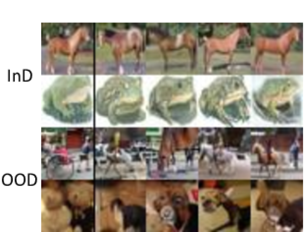
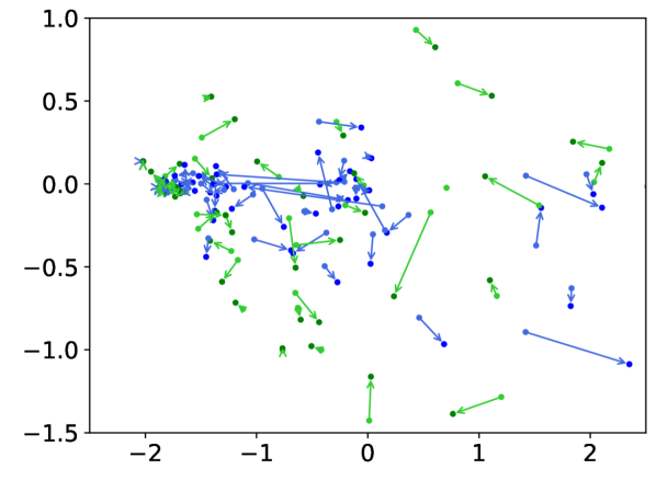
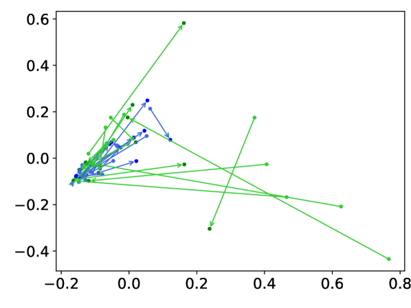
Figure 10: Three figures show the influence on the different levels under DDP, including the image space, the first and the fourth feature spaces of a ResNet18 respectively. In the first image, the first column is the original input and the remaining is the augmentation results of them. In the last two images, the blue and green arrow is the feature change of InD data and OOD data respectively under DDP after dimensionality reduction using PCA.

In Figure 10, we show the augmentation results of different inputs using DDP and the influence of DDP on the different feature spaces of a pre-trained ResNet18. The augmentation results have a more obvious semantic change for OOD input. For example, a rickshaw becomes a horse in Fig 10.1. On the other hand, the semantic information of the augmentation results of the InD data is relatively unchanged. Correspondingly, We can find that the change in low-level features (the first feature space, in Fig 10.2) is similar but the change in high-level semantic features (the fourth feature space, in Fig 10.3) becomes small when the input is InD and relatively big when the input is OOD.

Therefore, the low-level features concentrate on the pixel-level changes and do not differ much for the InD and OOD inputs. When we filter out the irrelevant information and focus on the semantic level changes, the change in the InD data is relatively small. This is because the interpolation operator can keep the InD input in the InD area. The effect of keeping the input in the InD area can only be observed in the high-level feature spaces. This explains why we cannot solve the OOD detection task with a single diffusion model and shows the information extraction ability of discriminator models.

A.4.2 Different type of input

In Figure 11, we use real cases to show the relationship between different inputs and the maximum value of the logit (the confidence). For the first group, these InD data change in the InD area. Although the images change obviously in the pixel level under DDP, the confidence results remain largely stable. For the second group, these OOD data contain no class-related features and DDP pull them to the high-density area of the training data. Therefore, the confidence results increase generally. For the third group, these OOD data contain sparse class-related features, but these features are captured by the discriminator by coincidence. These are two examples of the overconfidence problem. However, these sparse class-related features cannot be maintained under DDP. There is a significant drop in the confidence results. All these results support the analysis in Section 3.4.

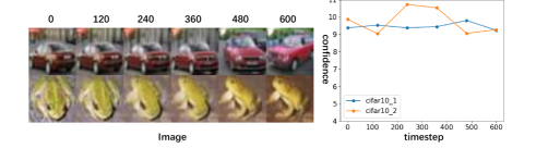
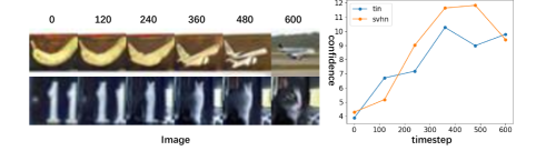
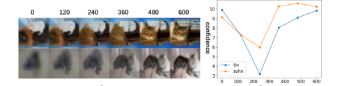
Figure 11: Changes in images under DDP and the corresponding confidence results.

A.5 Experiment setting

For CIFAR10/100, we employ a pre-trained ResNet18 [34] and the diffusion model from DDPM. To obtain a conditional diffusion model, we add an additional condition embedding and concatenate it with the timestep embedding. For ImageNet, we use a pre-trained ResNet50 and a pre-trained latent diffusion model [35]. The main hyperparameters for our diffusion-based OOD detection:

Model	Hyperparam	Value
		CIFAR	ImageNet
diffusion	timestep	300	600
	guidance scale	3.0	6.0
	repeat size	4	4
ResNet	feature space	logit	feature5
	threshold	n/a	0.3

A.6 FPR@95 result

In Table 4 and 5, we provide the FPR@95 results, which are highly consistent with the AUROC results in the main paper. We observe that the advantages in FPR@95 are more pronounced than in AUROC. The mean FPR@95 on CIFAR10 decreased from the previous SOTA value of 38.32 to 27.33, and the mean FPR@95 on CIFAR100 decreased from 75.12 to 59.08. This is because the FPR@95 is more sensitive to the OOD data with high confidence. The OOD data with high confidence are more likely to cause overconfidence problems. Our method can effectively reduce the confidence of OOD data, so the advantages are more obvious in FPR@95.

Table 4: The FPR@95 results of different methods on CIFAR10 and CIFAR100. The higher results are better and the bold results are the best in each case.

InD	cifar10					cifar100
OOD	cifar100	tin	svhn	texture	place	cifar10	tin	svhn	texture	place
ODIN	58.72	55.52	67.46	50.53	50.07	83.1	77.67	89.72	78.37	81.2
EBO	51.31	44.89	44.69	48.01	41.74	81.47	76.06	82.75	82.43	80.66
ReAct	53.34	46.73	48.83	49.66	43.84	86	78.37	80.99	75.23	82.98
MLS	52.04	45.37	44.55	48.56	42.72	81.27	75.25	82.39	82.46	80.22
VIM	56.11	52.19	14.29	21.03	47.99	87.75	82.46	82.58	56.1	83.83
KNN	52.17	46.36	33.43	45.6	43.4	82.27	73.82	74.37	66.4	78.74
Diff(ours)	35.95	28.52	19.6	23.75	28.82	71.53	52.38	49.78	59.55	62.18

Table 5: The FPR@95 results of different methods on ImageNet and the mean and standard deviation of the results on CIFAR10, CIFAR100, and ImageNet. A higher mean value is better, while a lower standard variance is better. The best results are in bold.

InD	imagenet					cifar10		cifar100		imagenet
OOD/stat	species	inatur	texture	place	sun	mean	std	mean	std	mean	std
ODIN	80.49	42.04	45.44	61.85	53.82	56.46	6.37	82.01	4.32	56.73	13.73
EBO	82.61	53.73	52.43	66	58.8	46.13	3.26	80.67	2.42	62.71	11.03
ReAct	68.53	19.36	45.6	33.47	24.02	48.48	3.15	80.71	3.71	38.20	17.62
MLS	80.86	50.8	54.2	65.62	59.83	46.65	3.29	80.32	2.66	62.26	10.58
VIM	85.72	73.01	13.05	85.61	83.7	38.32	17.20	78.54	11.38	68.22	27.98
KNN	90.23	63.52	19.43	84.66	75.68	44.19	6.11	75.12	5.34	66.70	25.30
Diff(ours)	55.81	13.45	47.16	32.9	31.63	27.33	5.49	59.08	7.70	36.19	14.52

A.7 Ablation study

An interesting additional ablation study involves the threshold of features, which has been shown to be useful for the large ImageNet dataset in previous work ReAct. In Figure 12, we find that 0.3 is the optimal choice for diffusion-based OOD detection, which differs from ReAct, where the optimal choice is around 1.0.

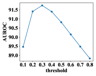
Figure 12: the AUROC results obtained under different thresholds on ImageNet.

A.8 Project License

Here, we present the GitHub repository addresses and the project licenses for the main open-source projects used in this paper.

name	GitHub	license
DDPM	https://github.com/hojonathanho/diffusion	n/a
DDIM	https://github.com/ermongroup/ddim	MIT license
Latent Diffusion	https://github.com/CompVis/latent-diffusion	MIT license
OpenOOD	https://github.com/Jingkang50/OpenOOD	MIT license

References

- Xin et al. [2018] Yang Xin, Lingshuang Kong, Zhi Liu, Yuling Chen, Yanmiao Li, Hongliang Zhu, Mingcheng Gao, Haixia Hou, and Chunhua Wang. Machine learning and deep learning methods for cybersecurity. Ieee access, 6:35365–35381, 2018.
- Latif et al. [2018] Siddique Latif, Muhammad Usman, Rajib Rana, and Junaid Qadir. Phonocardiographic sensing using deep learning for abnormal heartbeat detection. IEEE Sensors Journal, 18(22):9393–9400, 2018.
- Guo et al. [2020] Peng Guo, Zhiyun Xue, Zac Mtema, Karen Yeates, Ophira Ginsburg, Maria Demarco, L Rodney Long, Mark Schiffman, and Sameer Antani. Ensemble deep learning for cervix image selection toward improving reliability in automated cervical precancer screening. Diagnostics, 10(7):451, 2020.
- Geiger et al. [2012] Andreas Geiger, Philip Lenz, and Raquel Urtasun. Are we ready for autonomous driving? the kitti vision benchmark suite. In 2012 IEEE conference on computer vision and pattern recognition, pages 3354–3361. IEEE, 2012.
- Wang et al. [2022] Haoqi Wang, Zhizhong Li, Litong Feng, and Wayne Zhang. Vim: Out-of-distribution with virtual-logit matching. In Proceedings of the IEEE/CVF Conference on Computer Vision and Pattern Recognition, pages 4921–4930, 2022.
- An and Cho [2015] Jinwon An and Sungzoon Cho. Variational autoencoder based anomaly detection using reconstruction probability. Special Lecture on IE, 2(1):1–18, 2015.
- Nalisnick et al. [2019] Eric Nalisnick, Akihiro Matsukawa, Yee Whye Teh, and Balaji Lakshminarayanan. Detecting out-of-distribution inputs to deep generative models using typicality. arXiv preprint arXiv:1906.02994, 2019.
- Nguyen et al. [2015] Anh Nguyen, Jason Yosinski, and Jeff Clune. Deep neural networks are easily fooled: High confidence predictions for unrecognizable images. In Proceedings of the IEEE conference on computer vision and pattern recognition, pages 427–436, 2015.
- Vahdat et al. [2021] Arash Vahdat, Karsten Kreis, and Jan Kautz. Score-based generative modeling in latent space. Advances in Neural Information Processing Systems, 34, 2021.
- Ho et al. [2022] Jonathan Ho, Tim Salimans, Alexey A Gritsenko, William Chan, Mohammad Norouzi, and David J Fleet. Video diffusion models. In ICLR Workshop on Deep Generative Models for Highly Structured Data, 2022.
- Liang et al. [2018] Shiyu Liang, Yixuan Li, and R Srikant. Enhancing the reliability of out-of-distribution image detection in neural networks. In International Conference on Learning Representations, 2018.
- Sun et al. [2022] Yiyou Sun, Yifei Ming, Xiaojin Zhu, and Yixuan Li. Out-of-distribution detection with deep nearest neighbors. arXiv preprint arXiv:2204.06507, 2022.
- Hsu et al. [2020] Yen-Chang Hsu, Yilin Shen, Hongxia Jin, and Zsolt Kira. Generalized odin: Detecting out-of-distribution image without learning from out-of-distribution data. In Proceedings of the IEEE/CVF Conference on Computer Vision and Pattern Recognition, pages 10951–10960, 2020.
- Sricharan and Srivastava [2018] Kumar Sricharan and Ashok Srivastava. Building robust classifiers through generation of confident out of distribution examples. arXiv preprint arXiv:1812.00239, 2018.
- Hendrycks et al. [2022] Dan Hendrycks, Andy Zou, Mantas Mazeika, Leonard Tang, Bo Li, Dawn Song, and Jacob Steinhardt. Pixmix: Dreamlike pictures comprehensively improve safety measures. In Proceedings of the IEEE/CVF Conference on Computer Vision and Pattern Recognition, pages 16783–16792, 2022.
- Sehwag et al. [2020] Vikash Sehwag, Mung Chiang, and Prateek Mittal. Ssd: A unified framework for self-supervised outlier detection. In International Conference on Learning Representations, 2020.
- Nalisnick et al. [2018] Eric Nalisnick, Akihiro Matsukawa, Yee Whye Teh, Dilan Gorur, and Balaji Lakshminarayanan. Do deep generative models know what they don’t know? arXiv preprint arXiv:1810.09136, 2018.
- Serrà et al. [2019] Joan Serrà, David Álvarez, Vicenç Gómez, Olga Slizovskaia, José F Núñez, and Jordi Luque. Input complexity and out-of-distribution detection with likelihood-based generative models. In International Conference on Learning Representations, 2019.
- Zhang et al. [2020] Yufeng Zhang, Wanwei Liu, Zhenbang Chen, Ji Wang, Zhiming Liu, Kenli Li, and Hongmei Wei. Out-of-distribution detection with distance guarantee in deep generative models. arXiv preprint arXiv:2002.03328, 2020.
- Jiang et al. [2022] Dihong Jiang, Sun Sun, and Yaoliang Yu. Revisiting flow generative models for out-of-distribution detection. In International Conference on Learning Representations, 2022.
- Ho et al. [2020] Jonathan Ho, Ajay Jain, and Pieter Abbeel. Denoising diffusion probabilistic models. In Advances in Neural Information Processing Systems, volume 33, pages 6840–6851, 2020.
- Song et al. [2021a] Jiaming Song, Chenlin Meng, and Stefano Ermon. Denoising diffusion implicit models. In International Conference on Learning Representations, 2021a.
- Ho and Salimans [2021] Jonathan Ho and Tim Salimans. Classifier-free diffusion guidance. In NeurIPS 2021 Workshop on Deep Generative Models and Downstream Applications, 2021.
- Shoemake [1985] Ken Shoemake. Animating rotation with quaternion curves. In Proceedings of the 12th annual conference on Computer graphics and interactive techniques, pages 245–254, 1985.
- Yang et al. [2022] Jingkang Yang, Pengyun Wang, Dejian Zou, Zitang Zhou, Kunyuan Ding, Wenxuan Peng, Haoqi Wang, Guangyao Chen, Bo Li, Yiyou Sun, et al. Openood: Benchmarking generalized out-of-distribution detection. arXiv preprint, 2022.
- Krizhevsky et al. [2017] Alex Krizhevsky, Ilya Sutskever, and Geoffrey E Hinton. Imagenet classification with deep convolutional neural networks. Communications of the ACM, 60(6):84–90, 2017.
- Netzer et al. [2011] Yuval Netzer, Tao Wang, Adam Coates, Alessandro Bissacco, Bo Wu, and Andrew Y Ng. Reading digits in natural images with unsupervised feature learning. 2011.
- Cimpoi et al. [2014] Mircea Cimpoi, Subhransu Maji, Iasonas Kokkinos, Sammy Mohamed, and Andrea Vedaldi. Describing textures in the wild. In Proceedings of the IEEE conference on computer vision and pattern recognition, pages 3606–3613, 2014.
- Zhou et al. [2017] Bolei Zhou, Agata Lapedriza, Aditya Khosla, Aude Oliva, and Antonio Torralba. Places: A 10 million image database for scene recognition. IEEE transactions on pattern analysis and machine intelligence, 40(6):1452–1464, 2017.
- Hendrycks et al. [2019] Dan Hendrycks, Steven Basart, Mantas Mazeika, Mohammadreza Mostajabi, Jacob Steinhardt, and Dawn Song. Scaling out-of-distribution detection for real-world settings. arXiv preprint arXiv:1911.11132, 2019.
- Huang and Li [2021] Rui Huang and Yixuan Li. Mos: Towards scaling out-of-distribution detection for large semantic space. In Proceedings of the IEEE/CVF Conference on Computer Vision and Pattern Recognition, pages 8710–8719, 2021.
- Xiao et al. [2010] Jianxiong Xiao, James Hays, Krista A Ehinger, Aude Oliva, and Antonio Torralba. Sun database: Large-scale scene recognition from abbey to zoo. In 2010 IEEE computer society conference on computer vision and pattern recognition, pages 3485–3492. IEEE, 2010.
- Fawcett [2006] Tom Fawcett. An introduction to roc analysis. Pattern recognition letters, 27(8):861–874, 2006.
- He et al. [2016] Kaiming He, Xiangyu Zhang, Shaoqing Ren, and Jian Sun. Deep residual learning for image recognition. In Proceedings of the IEEE conference on computer vision and pattern recognition, pages 770–778, 2016.
- Rombach et al. [2022] Robin Rombach, Andreas Blattmann, Dominik Lorenz, Patrick Esser, and Björn Ommer. High-resolution image synthesis with latent diffusion models. In Proceedings of the IEEE/CVF Conference on Computer Vision and Pattern Recognition, pages 10684–10695, 2022.
- Liu et al. [2020] Weitang Liu, Xiaoyun Wang, John Owens, and Yixuan Li. Energy-based out-of-distribution detection. Advances in Neural Information Processing Systems, 33:21464–21475, 2020.
- Sun et al. [2021] Yiyou Sun, Chuan Guo, and Yixuan Li. React: Out-of-distribution detection with rectified activations. Advances in Neural Information Processing Systems, 34:144–157, 2021.
- Song et al. [2023] Yang Song, Prafulla Dhariwal, Mark Chen, and Ilya Sutskever. Consistency models. arXiv preprint arXiv:2303.01469, 2023.
- Zhang and Agrawala [2023] Lvmin Zhang and Maneesh Agrawala. Adding conditional control to text-to-image diffusion models. arXiv preprint arXiv:2302.05543, 2023.
- Ramesh et al. [2021] Aditya Ramesh, Mikhail Pavlov, Gabriel Goh, Scott Gray, Chelsea Voss, Alec Radford, Mark Chen, and Ilya Sutskever. Zero-shot text-to-image generation. In International Conference on Machine Learning, pages 8821–8831. PMLR, 2021.
- Ramesh et al. [2022] Aditya Ramesh, Prafulla Dhariwal, Alex Nichol, Casey Chu, and Mark Chen. Hierarchical text-conditional image generation with clip latents. arXiv preprint arXiv:2204.06125, 2022.
- Austin et al. [2021] Jacob Austin, Daniel D Johnson, Jonathan Ho, Daniel Tarlow, and Rianne van den Berg. Structured denoising diffusion models in discrete state-spaces. Advances in Neural Information Processing Systems, 34:17981–17993, 2021.
- Kong et al. [2020] Zhifeng Kong, Wei Ping, Jiaji Huang, Kexin Zhao, and Bryan Catanzaro. Diffwave: A versatile diffusion model for audio synthesis. In International Conference on Learning Representations, 2020.
- Lam et al. [2021] Max WY Lam, Jun Wang, Dan Su, and Dong Yu. Bddm: Bilateral denoising diffusion models for fast and high-quality speech synthesis. In International Conference on Learning Representations, 2021.
- Nichol and Dhariwal [2021] Alexander Quinn Nichol and Prafulla Dhariwal. Improved denoising diffusion probabilistic models. In International Conference on Machine Learning, pages 8162–8171. PMLR, 2021.
- Liu et al. [2022] Luping Liu, Yi Ren, Zhijie Lin, and Zhou Zhao. Pseudo numerical methods for diffusion models on manifolds. In International Conference on Learning Representations, 2022.
- Bao et al. [2022] Fan Bao, Chongxuan Li, Jun Zhu, and Bo Zhang. Analytic-dpm: an analytic estimate of the optimal reverse variance in diffusion probabilistic models. In International Conference on Learning Representations, 2022.
- Salimans and Ho [2022] Tim Salimans and Jonathan Ho. Progressive distillation for fast sampling of diffusion models. In International Conference on Learning Representations, 2022.
- Dhariwal and Nichol [2021] Prafulla Dhariwal and Alexander Nichol. Diffusion models beat gans on image synthesis. Advances in Neural Information Processing Systems, 34, 2021.
- Song et al. [2021b] Yang Song, Jascha Sohl-Dickstein, Diederik P Kingma, Abhishek Kumar, Stefano Ermon, and Ben Poole. Score-based generative modeling through stochastic differential equations. In International Conference on Learning Representations, 2021b.
- Chen et al. [2018] Ricky TQ Chen, Yulia Rubanova, Jesse Bettencourt, and David K Duvenaud. Neural ordinary differential equations. Advances in neural information processing systems, 31, 2018.
- Dupont et al. [2019] Emilien Dupont, Arnaud Doucet, and Yee Whye Teh. Augmented neural odes. Advances in Neural Information Processing Systems, 32, 2019.
- Ge et al. [2017] ZongYuan Ge, Sergey Demyanov, Zetao Chen, and Rahil Garnavi. Generative openmax for multi-class open set classification. arXiv preprint arXiv:1707.07418, 2017.
- Neal et al. [2018] Lawrence Neal, Matthew Olson, Xiaoli Fern, Weng-Keen Wong, and Fuxin Li. Open set learning with counterfactual images. In Proceedings of the European Conference on Computer Vision (ECCV), pages 613–628, 2018.
- Marek et al. [2021] Petr Marek, Vishal Ishwar Naik, Vincent Auvray, and Anuj Goyal. Oodgan: Generative adversarial network for out-of-domain data generation. arXiv preprint arXiv:2104.02484, 2021.
- Du et al. [2022] Xuefeng Du, Zhaoning Wang, Mu Cai, and Yixuan Li. Vos: Learning what you don’t know by virtual outlier synthesis. arXiv preprint arXiv:2202.01197, 2022.