Magnetic activities and parameters of 43 flare stars in the GWAC archive

Abstract

In the archive of the Ground Wide Angle Camera (GWAC), we found 43 white light flares from 43 stars, among which, three are sympathetic or homologous flares, and one of them also has a quasi-periodic pulsation with a period of $13.0\pm 1.5$ minutes. Among these 43 flare stars, there are 19 new active stars and 41 stars that have available TESS and/or K2 light curves, from which we found 931 stellar flares. We also obtained rotational or orbital periods of 34 GWAC flare stars, of which 33 are less than 5.4 days, and ephemerides of three eclipsing binaries from these light curves. Combining with low resolution spectra from LAMOST and the Xinglong 2.16m telescope, we found that $L_{\rm H\alpha}/L_{\rm bol}$ are in the saturation region in the rotation-activity diagram. From the LAMOST medium-resolution spectrum, we found that Star #3 (HAT 178-02667) has double H$\alpha$ emissions which imply it is a binary, and two components are both active stars. Thirteen stars have flare frequency distributions (FFDs) from TESS and/or K2 light curves. These FFDs show that the flares detected by GWAC can occur at a frequency of 0.5 to 9.5 yr^-1. The impact of flares on habitable planets was also studied based on these FFDs, and flares from some GWAC flare stars may produce enough energetic flares to destroy ozone layers, but none can trigger prebiotic chemistry on their habitable planets.

1 Introduction

Stellar flares are powerful explosions that can occur on stars ranging from A-type (Balona 2015) to even L-type (Paudel et al. 2020). Solar flares have been well studied based on space observatories, such as the Geostationary Operational Environmental Satellite (GOES), Solar Dynamics Observatory (Pesnell et al. 2012), the the Reuven Ramaty High Energy Solar Spectroscopic Imager (Lin et al. 2002), and the Interface Region Imaging Spectrograph (De Pontieu et al. 2021), etc. They may release explosive energy via magnetic reconnection (Zweibel & Yamada 2009) and released by electromagnetic radiations from radio to $\gamma$-ray (e.g. Bai & Sturrock 1989; Osten et al. 2005), and coronal mass ejections (CMEs) (e.g. Kahler 1992). The stronger the flare, the more likely it is to produce a CME (Li et al. 2021). Since the Sun belongs to an ordinary incative star of G2V type (Balona 2015), it is worthy of investigating stellar flare activities from most kinds of active stars to understand whether stellar flares may experience similar physics to solar flares or not.

Statistical studies of stellar flares have been conducted based on many survey projects. In the space, the Kepler (Borucki et al. 2010) provided photometric data with high precision, which can be used to study flare activities on stars across the H-R diagram with homogenous data for the first time (Balona 2015; Yang & Liu 2019). The Transiting Exoplanet Survey Satellite (TESS; Ricker et al. 2015) surveys all the sky, covering much wider than Kepler/K2. As a result, many new flare stars with high photometric precision can be studied (e.g. Tu et al. 2021; Howard & MacGregor 2022). On the ground, the Next Generation Transit Survey (Wheatley et al. 2018), ASAS-SN (Shappee et al. 2014), Evryscope (Law et al. 2015), and so on, have achieved fruitful results on flare study (e.g. Jackman et al. 2021; Rodríguez Martínez et al. 2020; Howard et al. 2020a).

Rotation is a key parameter to decide the activity of a star, e.g., factor in inducing stellar flares. Some indicators of stellar activity show the well-known activity-rotation relationship with a critical period. For stars with rotation periods smaller than the critical period, the activity is saturated, otherwise the activity decreases as the rotation period increases. The stellar activity-rotation relationship has been identified by X-ray (Pizzolato et al. 2003), white light (Raetz et al. 2020), Ca II H & K (Zhang et al. 2020) and H$\alpha$ (Newton et al. 2017; Yang et al. 2017; Lu et al. 2019).

Pre-main sequence stars often show intense flare activities, which result in the hot plasma escaping and then angular momentum losses (Colombo et al. 2019). Magnetized stellar winds also can brake stellar rotations (Gallet & Bouvier 2013). Therefore, with rotation slowing dwon, flare activity decreases with age (Ilin et al. 2021; Davenport et al. 2019). The same mechanism is also proposed to occur in a close binary system (Yakut & Eggleton 2005). Magnetic braking may result in the shrink of the orbit period, and then make both components in the binary synchronously spin up (Qian et al. 2018), and thus the more frequent flare activity.

Flare activity may play key roles in affecting habitability of nearby planets in the way of UV irradiation and CMEs. For M stars, on one hand, M stars can not produce enough UV photos (Rimmer et al. 2018), so UV radiation from frequent flares is needed to contribute to the creation of primitive life (Xu et al. 2018); on the other hand, UV radiation from frequent flares can also destroy ozone layers and life would not survive (Tilley et al. 2019). Moreover, CMEs from flares can erode even the whole atmosphere of a habitable exoplanet (Lammer et al. 2007; Atri & Mogan 2021).

In this paper, we present 43 stellar white light flares in the archive of the Ground-based Wide Angle Cameras (GWAC). GWAC is one of ground facilities of the Space-based multi-band astronomical Variable Objects Monitor (SVOM; Wei et al. 2016), in order to detect the optical transits with a cadence of 15 seconds (Xin et al. 2021; Wang et al. 2020). We searched all light curves during December 2018 and May 2019 of stars with Gaia G $<15$ mag, and found 43 stellar flares form 43 stars. In Section 2, we will introduce the light curves we used; In Section 3, we will show three sympathetic or homologous flares and one quasi-periodic pulsation; In Section 4, four binaries are studied; In Section 5, we will present the rotation-activity relationship by H$\alpha$ emissions; The impacts of flares on habitable planets are discussed in Section 6; At last, Section 7 is conclusion.

2 Light Curves

The GWAC stellar flare candidates between December 2018 and May 2019 were obtained by the program given by Ma (2019), which tried to find flares by a wavelet algorithm. We inspected all candidates by eye and found 43 stellar flares from 43 stars. We checked these stars in SIMBAD and the International Variable Star Index , and found that 19 stars have never been reported as flare stars or having H$\alpha$ emissions, thus new active stars. All GWAC flares are listed in Table LABEL:tab:gwacflare. We searched their light curves from the MAST site , and found TESS and K2 light curves for 39 stars. For the stars that have both K2 and TESS light curves, the TESS light curves were used. For TESS light curves, we noticed that there are several products for the same sector from different groups, and if light curves of the Science Processing Operations Center (SPOC; Jenkins et al. 2016) are available, then use them, otherwise use light curves of TESS-SPOC (Caldwell et al. 2020). The light curves of simple aperture photometry (SAP) were used, because pre-search data conditioning (PDC) ones may remove real variabilities (Vida et al. 2019). We also checked the PDC light curves of our sample, and found they work as well as SAP ones. Star #3 (HAT 178-02667), #14 (1RXS J075908.2+171957), #24, and #38 (BX Ari) have no available light curves in the MAST site. Star # 3 (HAT 178-02667) is not observed by TESS, and Star #24 is contaminated by a very bright star 13 arcseconds away. As a result, we obtained light curves of Star #14 (1RXS J075908.2+171957) and #38 (BX Ari) from their Full Frame Images. In sum, 41 of 43 GWAC flare stars have TESS or K2 light curves. The TESS sectors and K2 campaigns used in this work are listed in Table 2.

2.1 Flare Detection and Rotational Periods

To detect flares, for each light curve of a TESS sector or K2 campaign, we used a cubic B-spline to fit the out-of-flare variability, and then removed the fitted B-spline from the light curve. In the residual of a light curve, flares can be detected by residual fluxes larger than 3$\sigma$, where $\sigma$ is the standard deviation of the out-of-flare residual. At last, the stellar rotational period was calculated from the out-of-flare variability. Detailed steps are as follows:

• Step 1: Remove the points with fluxes greater than the top $2\%$ flux from the light curve ($l_{0}$), the new light curve is denoted as $l_{1}$.

• Step 2: Calculate the Lomb-Scargle periodogram (LS; Lomb 1976; Scargle 1982) of $l_{1}$ using the code LombScargle in the python package astropy.timeseries (Astropy Collaboration et al. 2013, 2018), then determine the preriod $P_{0}$ of the light curve.

• Step 3: A cubic B-Spline curve with a knot interval of 0.1$P_{0}$ is used to fit the $l_{1}$, and denote the new B-Spline as $S_{1}$ and $R_{1}=l_{1}-S_{1}$. Calculate the standard deviation $\sigma_{1}$ of $R_{1}$, and remove the points with $R_{1}$ values greater than 2$\sigma_{1}$. The new light curve is denoted as $l_{2}$, and $l_{1}:=l_{2}$. Then repeat this step again, and obtain the the standard deviation $\sigma$ of $l_{1}$, B-Spline $S$, and $R=l_{0}-S$ for finding flares.

• Step 4: A flare is detected from $R$ if there are at least 3 (for curves of 2 minutes cadence) or 2 (for curves of 30 minutes cadence) successive fluxes greater than 2$\sigma$ and the flare peak is greater than 3$\sigma$.

• Step 5: After all flares were removed from the light curve, the rotational period $P$ was calculated from the out-of-flare light curve by LS.

Figure 1 shows the results of our algorithm. In the upper panel, the red line is the fitted cubic B-spline, and flares detected are shown in blue. All flares detected were inspected by eye, and finally obtained 931 flares.

The rotational periods of 31 stars were obtained by the above algorithm, and the periods of 3 eclipsing binaries were calculated in Section 4. Star #3 (HAT 178-02667) is not observed by TESS and K2, but it has a period of 1.717885 days from Hartman et al. (2011), which may be the orbital period (see Section 4 for details), so there are total 35 GWAC flare stars have periods. Among the 31 stars that have rotational periods, 30 stars have periods less than 5.4 days, and the left one has a period of about 10.42 days, and thus all are rapid rotators.

Flares and periods detected in TESS and K2 light curves by the above algorithm, the 43 GWAC flare light curves and the flare movie of Star #4 (G 176-59), #7 LSPM J1542+6537), #28 (G 235-65), and #39 (1RXS J064358.4+704222) are all given in https://nadc.china-vo.org/res/r101145/.

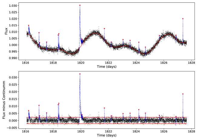
Figure 1: Upper panel: the black dots are from a part of the light curve of Star #1 (TIC 141533801) in Sector 19 of TESS. The red curve is the fitted cubic B-Spline curve. Lower panel: the black dots are the residuals of the fluxes minus the fitted cubic B-Spline curve, and the two red lines indicate $\pm 3\sigma$ positions. In both panels, the detected flares are shown in blue lines and their peaks are indicted by red dots.

2.2 Flare Energy

The equivalent duration (ED) (Gershberg 1972) was used to calculate a flare energy. ED is defined as: $\sum_{i}\frac{\bigtriangleup f_{i}}{f}\times\bigtriangleup t$, where, $\bigtriangleup f_{i}$ is a flux variation at time $t_{i}$ in the flare, $f$ is the quiescent flux and $\bigtriangleup t$ is the cadence. Then the flare energy is $E=ED\times f$.

GWAC has no filter, and the Gaia $G$ photometry of Gaia DR3 (Gaia Collaboration 2022) was used to calibrate the GWAC photometry by the GWAC pipeline, with a photometric accuracy better than 0.1 mag. Thus, we used the Gaia $G$ band filter and passband zero to calculate the quiescent flux $f$ of a GWAC flare star. The Gaia $G$ band filter was from Riello et al. (2021), the Vega spectrum was from Castelli & Kurucz (1994), and the Gaia $G$ magnitude of Vega was set 0.03 mag (Jordi et al. 2010). As a result, the passband zero $p_{0}$ of Gaia $G$ band is $9.12\times 10^{-6}$ erg cm^-2 s^-1.

The distances of GWAC flare stars were calculated from parallaxes of Gaia DR3, but there are three stars (Star #8 (HAT 149-01951), #14 (HAT 149-01951), and #29 (HAT 149-01951)) without available parallaxes in Gaia DR3. Then we used the equation of $M_{Ks}=1.844+1.116(V-J)$ given by Raetz et al. (2020), and $d=10^{0.2(M_{Ks}-Ks-5)}$ in pc to calculate their distances, where Ks and J are from 2MASS (Skrutskie et al. 2006), and V is from APASS (Henden et al. 2015). As a result, the quiescent flux in the $G$ band of a star is: $f=\pi d^{2}p_{0}10^{-0.4G}$ erg s^-1.

To obtain flare energies of TESS flares, the TESS response function and the passband zero from Sullivan et al. (2017) were used. The observed quiescent flux $f_{o}$ of a star in the TESS passband was the median value of its light curve multiplied by the TESS passband zero. Thus the the quiescent flux is $f=\pi d^{2}f_{o}$.

Two stars: Star #15 (HAT 307-06930) and #36 (CU Cnc) only have K2 light curves. Then the formulae (1) - (6) in Shibayama et al. (2013) were used to calculate quiescent fluxes in the Kepler passband, with the surface temperatures and stellar radii from Huber et al. (2016).

We assumed the fare energy was from a blackbody radiation with a temperature of 9000 K, and then used observed flare energies in Gaia $G$, TESS or $K2$ filters to calculate whole white light flare energies, which should be lower than the true released flare energies (e.g. Hawley & Pettersen 1991; Kretzschmar 2011).

2.3 Spectra

The Guoshoujing Telescope (the Large Sky Area Multi-Object Fiber Spectroscopic Telescope, LAMOST; Cui et al. 2012) can obtain 4000 spectra in one exposure, and is located at the Xinglong Observatory, the same place as GWAC and the 2.16m telescope. In LAMOST DR8 , there are about 11 million low-resolution spectra (LRS, $R\sim 1800$) and 6 million medium-resolution spectra (MRS, $R\sim 7500$). We searched spectra of GWAC flare stars in LAMOST DR8, and obtained available LRS for 25 stars, and MRS for 13 stars. Because 11 stars have available both LAMOST LRS and MRS, there are 27 stars have LAMOST spectra. We also obtained LRS of another 7 flare stars by the 2.16m telescope with the instrument G5. The spectral resolution is about 2.34 Å pixel^-1, and the wavelength coverage is 5200 Å- 9000 Å(Zhao et al. 2018). In sum, 32 of 43 flare stars have LSR, and 7 have LAMOST MRS.

The spectroscopic standards from Kirkpatrick et al. (1991) were used to assign spectral types of M stars that have LRS from LAMOST or the 2.16m telescope. For stars that have spectral types earlier than M0, their spectral types are from LAMOST DR8.

The Color-Magnitude Diagram (CMD) of flare stars with their spectra types are shown in Figure 2, where Gaia $G$, parallax $\varpi$ ( in milliarcsecond), $G_{bp}-G_{rp}$ are from Gaia DR3, and the absolute magnitude $M_{G}=G+5{\rm log}_{10}(\varpi)-10$. For 32 stars that have LRS, their H$\alpha$ are all shown in emission, which indicate they are all active stars. Among them, thirty-one stars were assigned spectral types and are shown in different symbols and colors in Figure 2. Star #21 was assigned a spectral type of M3, but with a bluer color in Figure 2. We found that its $ruwe=2.478$ in Gaia DR3, which implies that there may be some astrometric problems or it is not a single star, thus the Gaia photometry is unreliable. Star #18 (DR Tau) is not in Figure 2, because it is a T Tauri star (Chavarria-K. 1979), and there is no available absorption line in its spectrum for spectral classification.

For the other 11 stars without available spectra in this paper, their spectral types were also assigned by their $G_{bp}-G_{rp}$ in Figure 2. Among them, Star #9 (2MASS J04542368+1709534; Herczeg & Hillenbrand 2014), #23 (1RXS J101627.8-005127; Zickgraf et al. 2005), #27 (1RXS J120656.2+700754; Christian et al. 2001), #28 (G 235-65; Reid et al. 2004), #30 (1RXS J082204.1+744012; Fleming et al. 1988), and #35 (1RXS J075554.8+685514; Zickgraf et al. 2005) had been identified as active stars in the literature.

Figure 2: The Color-Magnitude Diagram (CMD) of flare stars with their spectral types. $M_{G}$ is the absolute magnitude of Gaia $G$. $G$, $G_{bp}$ and $G_{rp}$ are from Gaia DR3. The 31 stars that have LRS are shown in different symbols and colors for different spectral types. The black dots are the stars that have not available spectra in this paper.

In sum, there are one G type star, four K type stars, thirty-seven M type stars, and one T Tauri in our sample. Figure 3 shows the distribution of spectral types of GWAC flare stars, except one T Tauri (Star #18; DR Tau).

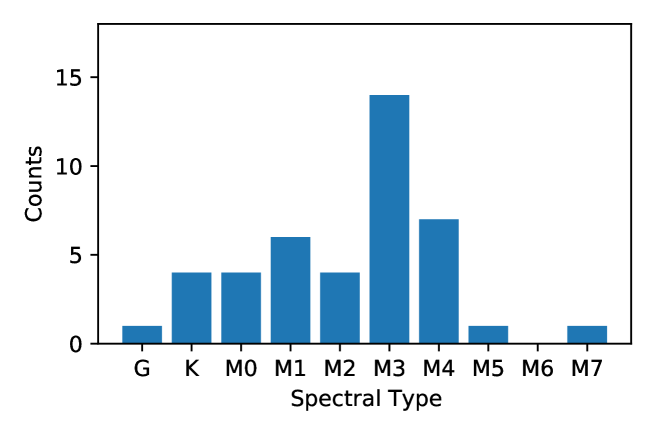
Figure 3: The distribution of spectral types of GWAC flare stars, except one T Tauri (Star #18; DR Tau).

To calculate the H_α emission luminosity $L_{\rm H_{\alpha}}$, the Sérsic function (Sersic 1968) was used to fit H_α emission profiles. The function is: $F(\lambda)=A_{0}\exp(Z^{A_{3}}/A_{3})+A_{4}+A_{5}\lambda$, where $Z=|(\lambda-A_{1})/A_{2}|$, $\lambda$ is wavelength in Å, and $A_{i}$, $i=0,\cdots,5$ are coefficients to be fitted. The wavelength range was set to $6564.61\pm 20$ Å(6564.61 Åis the vacuum wavelength of H$\alpha$), and the LAMOST spectral luminosity of H$\alpha$: $L^{\prime}_{\rm H_{\alpha}}=\int_{6544.61}^{6584.61}A_{0}\exp(Z^{A_{3}}/A_{3})d\lambda$. The fluxes of LAMOST spectra are not calibrated, but there is only a constant ratio between each spectrum and its true flux. For each star that has LAMOST LRS, we calculated its spectral flux $f_{L}$ from its LRS spectrum in the SDSS r^′ filter (Fukugita et al. 1996), and its observed flux $f_{A}$ from r^′ given by APASS (Henden et al. 2015). Then its $L_{\rm H\alpha}=L^{\prime}_{\rm H\alpha}*f_{A}/f_{L}$.

To obtain the quiescent bolometric luminosity $L_{\rm bol}$ of a star, photometric data from r^′, g^′ and i^′ of APASS (Henden et al. 2015), J, H, and K_s of 2MASS (Skrutskie et al. 2006), and W1, W2, W3, and W4 of WISE (Jarrett et al. 2011) for each star, were fitted by a blackbody irradiation function. In the calculation, the reference wavelengths and the zero points of all filters were from the SVO Filter Profile Service (Rodrigo & Solano 2020). Finally, $L_{\rm H\alpha}/L_{\rm bol}$ can be obtained. $L_{\rm H\alpha}/L_{\rm bol}$ that can be calculated from spectra are listed in Table 3. Because one star can have several LAMOST spectra, and one spectra has one $L_{\rm H\alpha}/L_{\rm bol}$, so there are several $L_{\rm H\alpha}/L_{\rm bol}$ for a star in Table 3.

The information of GWAC flare stars with their GWAC flares are given in Table LABEL:tab:gwacflare.

3 Flare Profiles

3.1 Sympathetic or homologous flares

Based on an enormous amount of observations, solar flares are well known to be produced by magnetic reconnections in active regions (ARs; Toriumi & Wang 2019). Solar ARs are the regions full of intense magnetic fields with complex morphologies (McIntosh 1990; Sammis et al. 2000). Successive flares are often observed on the Sun and are identified as sympathetic activity from different regions with physical causal links (Pearce & Harrison 1990; Moon et al. 2002; Schrijver & Higgins 2015; Hou et al. 2020), or homologous ones occurring in the same AR (e.g. Louis & Thalmann 2021; Xu et al. 2014).

It is interesting that there are three pairs of flares successively appearing among the 43 GWAC samples as shown in Figure 4. Each pair of flares occurred following a similar profile of light curves in the interval of 20-50 minutes. The morphology of the light curves during a flare may reflect the release processes of magnetic energies, and manifest complex magnetic topology of the intense magnetic fields. The successive occurrence of three pairs of stellar flares indicate that the cool stars may share the similar physical magnetic explosions to those sympathetic flares or homologous ones happening on the Sun. With the development of future imaging observations for the other stars, it is anticipated to unveil these possibly universal physical mechanisms.

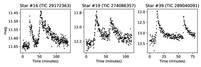
Figure 4: Successive flares from Star #16 (TIC 29172363), #19 (TIC 274086357; 1RXS J031750.1+010549), and #39 (TIC 289040091; 1RXS J064358.4+704222).

3.2 Quasi-periodic pulsation

Quasi-periodic pulsations (QPPs) are very common phenomenons in solar flares (Van Doorsselaere et al. 2016; Simões et al. 2015; Kupriyanova et al. 2010), but QPPs in stellar white light flares are still rare (Howard & MacGregor 2022; Pugh et al. 2016). More than a dozen of mechanisms were suggested to trigger QPPs (Kupriyanova et al. 2020). Coronal loop lengths can be derived from periods of QPPs from some mechanisms with some theoretical considerations (Ramsay et al. 2021). The periods of QPPs in white light curves are of tens minutes (Ramsay et al. 2021; Pugh et al. 2016), but at short cadence (20 seconds) of TESS, QPP periods less than 10 minutes were also found (Howard & MacGregor 2022).

GWAC has a cadence of 15 seconds, shorter than TESS, and make it possible to find QPPs with short periods in GWAC white light flares. One flare occurring on Star #16 (TIC 29172363) was found to indicate a QPP process as shown by the red light curve in the left panel of Figure 5. The function $f(t)=A_{0}\times\exp(A_{1}t)+A_{2}$ was used to fit the background of the QPP signal, and shown by the blue curve in the left panel of Figure 5. Here, $A_{0},A_{1}$ and $A_{2}$ are parameters to be fitted, and $t$ is time in seconds. According to the light curve after subtracting the background information, a character manifested by QPP process is shown in the middle panel of Figure 5, and is analyzed by using the LS periodogram. The right panel of Figure 5 shows the periodogram result. A period of $13.0\pm 1.5$ minutes is obtained for the QPP process.

Figure 5: The QPP of Star #16 (TIC 29172363). Left panel: the QPP position in the flare is indicated in red. The blue curve is the fitted background. Middle panel: the QPP signal without background. The blue curve is the fitted QPP with a period of 13.0 minutes; Right panel: the LS periodogram of the QPP signal in the middle panel.

4 Binary and multiple systems

We inspected all GWAC flare stars in Aladin (Bonnarel et al. 2000) and Gaia DR3, and found that there are 11 binaries and one triple system. Among them, Star #27 (TIC 142979644; 1RXS J120656.2+700754), #32 (TIC 382379884) and #36 (EPIC 211944670; CU Cnc) hold close eclipsing binaries. To obtain periods of binaries, we fitted the eclipse minimum times by quadratic polynomials of light curves, and ephemerides were calculated by fitting the eclipse minimum times. The ephemerides (in BJD) of Star #27 (TIC 142979644; 1RXS J120656.2+700754), #32 (TIC 382379884) and #36 (EPIC 211944670; CU Cnc) are

$$T_{min}-2457000=1683.36653104(\pm 0.00002399)+4.17903758(\pm 0.00000027)E$$

,

$$T_{min}-2457000=2144.48865796(\pm 0.00010348)+0.45825824(\pm 0.00000316)E$$

, and

$$T_{min}-2454833=2306.95408506(\pm 0.00199451)+2.77147142(\pm 0.00001076)E$$

, respectively. Here, $E$ is the circle number, and $T_{min}$ is the eclipse minimum time. O - C diagrams and light curves in phase are shown in Figure 6. Star #36 (EPIC 211944670; CU Cnc) is a triple system in Gaia DR3, so its ephemerides may be disturbed by the third star.

The secondary eclipse minimum of Star #27 (TIC 142979644; 1RXS J120656.2+700754) deviate from the phase 0.5 in Figure 6, so it has an eccentricity. We used the formulae 1 and 2 in Lei et al. (2022) to calculate its eccentricity ($e$) and periastron angle ($\omega$). From our calculation, its secondary eclipse phase $\phi_{2}=0.518$ (its primary eclipse phase $\phi_{1}=0$), and the widths of the primary and secondary eclipses were determined by eye, which are $w_{1}\sim 0.0176$ and $w_{2}\sim 0.018$, respectively. Then, $e\cos(\omega)=\frac{\pi}{2}\left[\phi_{2}-\phi_{1}-0.5\right]=0.028274$ and $e\sin(\omega)=\frac{w_{2}-w_{1}}{w_{2}+w_{1}}\sim 0.011236$. As a result, $e\sim 0.03$ and $\omega\sim 0.387$.

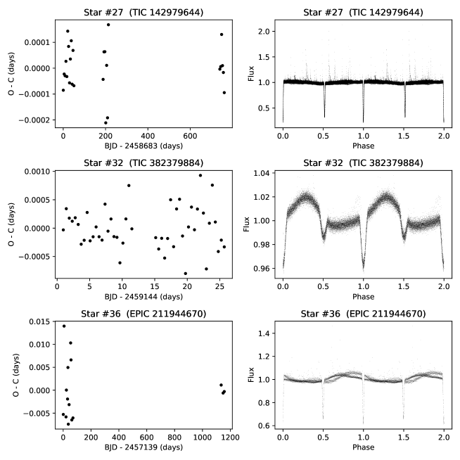
Figure 6: O - C diagrams and light curves in phases of Star #27 (TIC 142979644; 1RXS J120656.2+700754), #32 (TIC 382379884) and #36 (EPIC 211944670; CU Cnc) are shown in the left and right columns, respectively.

Star #3 (HAT 178-02667) has no Li I 6708 line in its LAMOST MRS as shown in the right panel of Figure 7, which implies that it is not a young star, and thus it unlikely holds a curcumstellar disk. Its $ruve=7.65$ in Gaia DR3 and there are double H$\alpha$ emissions in its LAMOST MRS as shown in the left panel of Figure 7, so it is likely a binary system and double H$\alpha$ emissions indicate both components are active stars. In Hartman et al. (2011), it has a period of 1.717885 days.

Figure 7: The LAMOST MRS of Star #3 (HAT 178-02667). Left panel: Double H$\alpha$ emissions of Star #3 (HAT 178-02667); Right panel: There is no Li I 6708. The positions of H$\alpha$ and Li I 6708 in vacuum are indicated in red lines.

5 H$\alpha$

H$\alpha$ is a very important indicator of stellar activity. Stars with strong H$\alpha$ emissions in their quiescent spectra are very likely to show strong flare activities (Kowalski et al. 2009). Figure 8 shows the relationship between H$\alpha$ luminosity from 44 spectra of 21 M dwarfs and $Ro=P_{\rm rot}/\tau$, where $P_{\rm rot}$ is the stellar rotational period and $\tau$ is the convective turnover time calculated from Equation 10 in Wright et al. (2011). For M type stars, their $L_{\rm X}/L_{\rm bol}$ shows saturation (e.g. Wright et al. 2018; Pizzolato et al. 2003) and even supersaturation (e.g. Jeffries et al. 2011) for rapid rotators. Compared to Figure 7 in Newton et al. (2017), our sample stars are all rapid rotators, and in the saturation region as shown In Figure 8.

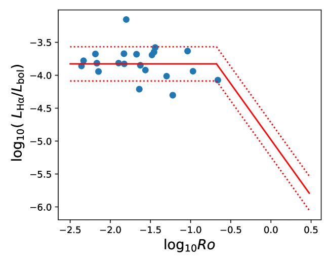
Figure 8: The relationship between $Ro$ and $L_{\rm H\alpha}/L_{\rm bol}$. The red line and dotted lines are the relationship and 1$\sigma$ contours given in (Newton et al. 2017).

6 Habitablity

Stellar activity is a double-edged sword for life on a habitable planet. On one hand, flare activities can contribute the generation and development of life (Rimmer et al. 2018), on the other hand erode and even destroy the ozone of a habitable-zone exoplanet (Tilley et al. 2019). We used Equation 10 in Günther et al. (2020) to delineate ”abiogenesis zone,” which means the flare frequency in this zone can contribute the prebiotic chemistry and then promote life generation.

The flare frequency distribution (FFD) is the cumulative flare energy frequency in per day (Gershberg 1972; Günther et al. 2020), and often used to show how often a flare energy higher than a given value is. We obtained FFDs of 13 single stars with more than 20 flares detected in TESS or $K2$ light curves, and a power law function ${\rm log}_{10}(\nu)=\alpha{\rm log}_{10}(E_{\rm bol})+\beta$ was used to fit each FFD, where $\nu$ is the cumulative flare frequency in day^-1, $E_{\rm bol}$ is the flare energy in erg, $\alpha$ and $\beta$ are parameters to be fitted. We also calculated the flare frequency $\nu$ of the GWAC flare energy using the fitted $\alpha$ and $\beta$ for each star, and found GWAC flares can occur at a frequency of 0.5 to 9.5 yr^-1.

Flares with $E_{\rm bol}\geqslant 10^{34}$ erg can impact atmospheres of habitable planets. The cumulative flare frequency of $\nu\geqslant 0.4$ day^-1 can remove more than 99.99% of the ozone layer of a habitable-zone exoplanet as suggested by Tilley et al. (2019), and a more permissive frequency limit is $\nu\geqslant 0.1$ day^-1.Though the flare temperature of 9000 K is popularly used in literature, but the flare temperature can reach as high as 30000 K and even 42000 K (Howard et al. 2020b). In Figure 9, blue lines for a flare temperature of 9000 K, while pink lines for 30000 K. We can see that for the flare temperature of 9000 K, two stars (TIC 88723334 and TIC 416538839) produce flares with energies greater than $10^{34}$ erg in the highest frequencies, but still can not destroy ozone layers of their habitable planets. However, for the flare temperature 30000 K, almost all stars can produce energetic flares to destroy ozone layers of their habitable planets, except Star #28 (TIC 103691996).

Equation 10 in Günther et al. (2020) was also used to calculate the flare frequency limit for prebiotic chemistry. These frequency limits are shown by brown lines in Figure 9, and there is no star having enough high energetic flares to trigger prebiotic chemistry on its habitable planets.

Figure 9: FFDs of 13 flaring single stars with flare numbers greater than 20. The grey dots are the flare frequency obtained from TESS or $K2$ light curves, and their fitted power law functions are shown by blue lines for a flare temperature of 9000 K, while pink lines for 30000 K. The yellow line is log${}_{10}(E_{\rm bol})=34$, and $\nu=0.1$ and 0.4 are shown in cyan and green lines, respectively. The brown lines represent the abiogenesis zones for flare stars calculated by Equation 10 in Günther et al. (2020).

7 Conclusion

In this paper, we studied the 43 flares from 43 stars found in the GWAC archive between December 2018 and May 2019, by combining light curves from TESS and $K2$, spectra from LAMOST and the 2.16m telescope the Xinglong Observatory, and parallax and photometry from Gaia DR3, and obtained the following results:

1. We found 19 new active stars.

2. We found 3 sympathetic or homologous flares, which imply that the cool stars may share the similar physical magnetic explosions to those happening on the Sun.

3. We found a white light QPP in the sympathetic or homologous flare of Star #16 (RX J0903.2+4207) with a period of $13.0\pm 1.5$ minutes, which shows the advantage of GWAC with a cadence of 15 seconds in discovering white light QPPs with short periods.

4. Thirty-four stars have rotational or orbital periods less than 5.4 days and only one star has a period of $\sim$10.42 days.

5. Eleven stars are binaries and one is a triple system. The ephemerides of three binaries are calculated from their light curves, and one of them (Star #27; 1RXS J120656.2+700754) also has an eccentricity of $e\sim 0.03$. Star #3 (HAT 178-02667) has no light curve, but double H$\alpha$ emissions in its LAMOST medium-resolution spectrum imply a binary.

6. $L_{\rm H\alpha}/L_{\rm bol}$ shows that the rapid rotators in GWAC flare stars are in the saturation region in the rotation-activity diagram.

7. Some of GWAC flare stars may produce enough energetic flares to destroy the ozone layer, but none can trigger prebiotic chemistry on its habitable planet.

Big flares with amplitudes greater than 1 mag detected by GWAC, can trigger telescopes in the Xinglong Observatory to follow up. Some research results have been obtained based on these observations (Xin et al. 2021; Wang et al. 2021, 2022). In future, we will continue to analysis these big flares to study their generation mechanisms and impacts on habitable planets.

Table 1: GWAC flare stars

#	Name	Other Name	New	R.A. J2000	Decl. J2000	Dis	Gmag	bp-rp	SpT	Multi	Period	Date	Start	End	Flare Energy	ED
				degree	degree	pc	mag	mag			days	yyyymmdd	hhmmss	hhmmss	$\rm log_{10}(erg)$	seconds
1	TIC 141533801	PM J06521+7908		103.040098	79.14838	39.98	10.514	1.68	M0		5.20898(0.42182)	20190223	123107	141352	35.09(0.10)	4485
2	TIC 8688061	PM J09108+3127		137.701223	31.45744	27.04	12.506	2.653	M3		4.24599(0.27568)	20190225	134702	150947	33.6(0.17)	2028
3		HAT 178-02667	Y	131.491539	36.59261	96.88	13.465	2.391	(M2.5)	Binary	1.717885	20190225	134702	150947	34.69(0.47)	4626
4	TIC 253050844	G 176-59	Y	177.70409	45.56739	29.6	14.033	3.029	M4.5			20190403	144350	180450	33.82(0.59)	11285
5	TIC 392402786	BD+48 1958		174.352417	47.46249	33.47	10.034	1.687	M0	Binary	1.03001(0.01528)	20190403	144350	180450	34.98(0.09)	1851
6	TIC 416538839	StKM 2-809		183.914031	52.65242	25.1	11.373	2.608	M3		0.72597(0.00680)	20190403	144350	180450	34.3(0.13)	4151
7	TIC 334637014	LSPM J1542+6537		235.554214	65.61809	38.92	13.233	2.889	M4.5		0.61722(0.00399)	20190403	180612	205708	34.07(0.40)	5561
8	TIC 162673744	HAT 149-01951	Y	246.061458	48.39066	59.69	13.615	2.482	M3		1.63170(0.04786)	20190502	165833	200324	34.22(0.37)	4755
9	TIC 436680588	2MASS J04542368+1709534		73.598678	17.16485	143.62	16.617	2.365	(M2.5)	Binary		20190113	102051	134136	35.37(0.51)	9090
10	TIC 20161577	HAT 138-01877	Y	145.345992	43.97308	99.51	12.793	1.78	(M1)		3.13022(0.14959)	20190125	151425	170400	34.19(0.08)	746
11	TIC 88723334	G 196-3	Y	151.089429	50.38705	21.81	10.615	2.35	M2.5		1.31341(0.02628)	20190125	151425	201525	34.56(0.09)	4946
12	TIC 323688555	GJ 3537		137.413115	6.70305	23	12.081	2.629	M3		4.06548(0.30373)	20190224	135938	153823	33.36(0.10)	1068
13	TIC 318230983	HAT 140-00487	Y	162.861825	48.69546	79.05	11.429	1.817	M1		4.06913(0.25229)	20190124	175515	211330	35.53(0.19)	7433
14		1RXS J075908.2+171957		119.779882	17.32982	24.16	12.706	2.8	(M4)		0.48204(0.00411)	20190113	135650	185505	33.5(0.29)	2382
15	EPIC 210701183	HAT 307-06930	Y	55.739582	18.37965	132.82	14.414	2.184	M1		1.67409(0.01648)	20190112	102758	141043	34.75(0.69)	6870
16	TIC 29172363	RX J0903.2+4207		135.811479	42.12356	79.49	11.647	1.703	M0		1.49055(0.03069)	20190201	170000	193443	35.44(0.13)	7350
17	TIC 283729913		Y	63.455228	9.21321	104.41	14.03	2.222	M2.5			20190114	113000	140052	34.36(0.42)	3188
18	TIC 436614005	DR Tau		71.775897	16.97856	192.97	11.651	1.621	T Tau			20190114	101252	154952	36.71(0.24)	23321
19	TIC 274086357	1RXS J031750.1+010549	Y	49.457729	1.10221	151.67	12.219	1.38	K3		0.63653(0.01102)	20181223	125610	162440	35.72(0.29)	6484
20	TIC 427020004	HAT 307-01221	Y	49.572707	18.40566	94.92	11.693	1.495	K5		3.16524(0.22178)	20190111	120004	151035	35.22(0.09)	3200
21	TIC 114059158		Y	55.304975	20.85436	140.32	13.862	1.96	M3		0.31366(0.00193)	20181230	145636	162551	34.88(0.28)	4953
22	TIC 195188536	DF Cnc		128.870322	18.20561	49.23	12.906	2.376	M3		5.35280(0.62707)	20190112	144958	195145	34.11(0.15)	2810
23	TIC 77644831	1RXS J101627.8-005127		154.112263	-0.86091	60.15	12.329	2.136	(M1.5)		0.74709(0.00835)	20190114	155759	191159	34.58(0.11)	3307
24			Y	153.304236	2.80498	105.46	17.593	3.115	(M5)			20190213	170041	180211	34.04(0.27)	1780
25	TIC 374270454	1RXS J103715.4+020612	Y	159.314334	2.09753	71.84	11.829	1.951	M1		3.51123(0.28641)	20190106	175650	205650	34.59(0.06)	1491
26	TIC 142877499	G 236-81		176.772653	70.03285	30.62	13.093	2.856	(M4)	Binary	10.42161(0.9949)	20190121	153702	205732	34.73(0.54)	16582
27	TIC 142979644	1RXS J120656.2+700754		181.73505	70.13054	17.37	10.892	2.845	(M4)	Binary	4.17903758(0.00000027)	20190318	134018	190333	33.65(0.12)	1065
28	TIC 103691996	G 235-65		154.787606	66.49275	29.26	13.053	2.662	(M3.5)			20190216	164856	195511	34.14(0.37)	9772
29	TIC 99173696		Y	123.681926	46.84348	39.3	13.745	2.84	M4		1.78860(0.01522)	20190206	162410	185425	33.37(0.25)	1733
30	TIC 153858162	1RXS J082204.1+744012		125.533783	74.67285	47.66	12.264	2.266	(M3)		1.97116(0.05626)	20190121	154417	183817	34.00(0.24)	1297
31	TIC 270478293	LP 589-69	Y	34.197584	1.2126	31.51	12.476	2.532	M3		4.49044(0.33040)	20181224	120134	142234	33.31(0.21)	735
32	TIC 382379884		Y	45.066475	-3.04574	114.87	12.073	1.53	M0	Binary	0.45825824(0.00000316)	20190127	102150	140010	35.48(0.14)	4360
33	TIC 435308532	LP 413-19		54.392052	17.85	38.8	12.079	2.712	M3	Binary	0.47630(0.00278)	20190204	113935	131650	34.12(0.06)	890
34	TIC 440686488	V660 Tau		57.116786	23.30076	134.02	12.242	1.319	K5		0.23520(0.00104)	20190204	113935	131650	35.54(0.24)	5538
35	TIC 457100137	1RXS J075554.8+685514		118.972289	68.9069	29.2	13.056	2.844	(M4)		0.53285(0.00445)	20			33.18(0.16)	1077
36	EPIC 211944670	CU Cnc		127.906559	19.39428	16.65	10.576	2.861	M3.5	Triple	2.7714842(0.00001076)	20190101	145240	190810	33.96(0.09)	1565
37	TIC 224304406	1RXS J123415.2+481306		188.564232	48.21862	46.83	13.135	2.675	M3		0.94869(0.01295)	20190206	191205	221635	33.71(0.18)	1535
38		BX Ari		44.546799	20.50087	234.85	11.921	1.541	K3	Binary	2.83690(0.14557)	20181229	135121	163451	36.35(0.16)	6342
39	TIC 289040091	1RXS J064358.4+704222		100.994199	70.70326	59.56	13.348	2.402	M3		0.54374(0.00562)	20181215	162100	174019	34.42(0.62)	5981
40	TIC 16246712		Y	153.803156	37.86495	95.42	12.945	2.066	M1	Binary		20			34.78(0.14)	1756
41	TIC 445830121		Y	173.045411	52.09011	42.3	13.465	2.503	M3	Binary		20190106	210011	222626	33.59(0.48)	1790
42	TIC 197251248	G 9-38		134.558692	19.76258	5.15	11.966	3.777	M7	Binary	0.25397(0.00150)	20190211	150414	155014	32.51(0.15)	1704
43	TIC 316276917		Y	133.388088	56.78993	225.65	12.087	1.042	G7		0.65862(0.00688)	20181227	165728	211943	35.56(0.15)	1797

0.86 1, The bolometric flare energies were calculated from GWAC flares assuming a blackbody with a temperature of 9000 K. The fraction of the bolometric energy in the Gaia $G$ band is $\frac{f_{G}}{f_{\rm bol}}\approx 0.3$.
2, Spectral types in parentheses are assigned based on $G_{\rm rp}-G_{\rm bp}$.
3, The period of Star #3 is from Hartman et al. (2011).

Table 2: Data of which TESS Sector and K2 Campaign was used

Star #	Name	Sectors
1	TIC 141533801	19,20,26,40
2	TIC 8688061	21
3
4	TIC 253050844	22
5	TIC 392402786	22
6	TIC 416538839	22
7	TIC 334637014	14,15,16,17,21,22,23,24,41
8	TIC 162673744	23,24,25
9	TIC 436680588	(43),(44)
10	TIC 20161577	21
11	TIC 88723334	21
12	TIC 323688555	8,34,45
13	TIC 318230983	21
14		44,45,46
15	EPIC 210701183	4
16	TIC 29172363	21
17	TIC 283729913	5,23
18	TIC 436614005	(43),(44)
19	TIC 274086357	4,31
20	TIC 427020004	42,43
21	TIC 114059158	42,43,44
22	TIC 195188536	44,45
23	TIC 77644831	8,35,45
24
25	TIC 374270454	35,45
26	TIC 142877499	21
27	TIC 142979644	14,15,21,41
28	TIC 103691996	14,21,40,41
29	TIC 99173696	20
30	TIC 153858162	20,26,40,47,53
31	TIC 270478293	4,31
32	TIC 382379884	(4),31
33	TIC 435308532	42,43,44
34	TIC 440686488	42,43,44
35	TIC 457100137	20,26,40
36	EPIC 211944670	5,18
37	TIC 224304406	22
38		(42),(43),(44)
39	TIC 289040091	19,20,26
40	TIC 16246712	21
41	TIC 445830121	21,(22)
42	TIC 197251248	44,45
43	TIC 316276917	20

0.86 The TESS sectors in parentheses mean that the data of these sectors are not available for this work.

Table 3: H$\alpha$ luminosity.

Star #	R. A. J2000	Decl. J2000	$\lg(L_{\rm H\alpha}/L)$
	degree	degree
2	137.702323	31.457447	-3.78(+0.01),-3.79(+0.01),-3.58(+0.00)
4	177.704090	45.567390	-3.63(+0.01)
5	174.352814	47.462439	-5.05(+0.01)
6	183.914032	52.652434	-3.69(+0.00),-3.68(+0.00),-3.78(+0.01)
7	235.554210	65.618100	-3.15(+0.00)
8	246.061805	48.390525	-3.66(+0.01)
9	73.598465	17.162068	-4.22(+0.02)
11	151.089442	50.387056	-3.67(+0.01),-3.65(+0.00)
12	137.413190	6.703040	-3.63(+0.00),-3.64(+0.00),-3.68(+0.00)
13	162.861881	48.695440	-4.01(+0.01),-4.09(+0.01)
15	55.739577	18.379597	-3.83(+0.01),-3.92(+0.01),-3.94(+0.01)
16	135.811466	42.123555	-3.82(+0.01)
17	63.455420	9.213330	-4.30(+0.01)
18	71.775872	16.978558	-2.47(+0.01),-2.75(+0.01)
19	49.457706	1.102194	-3.80(+0.01)
20	49.572717	18.405648	-4.07(+0.02)
21	55.306192	20.854802	-3.48(+0.00),-4.60(+0.05),-3.56(+0.01),-3.83(+0.02)
22	128.870334	18.205612	-3.84(+0.01),-3.86(+0.01),-3.87(+0.01)
26	159.314354	2.097543	-4.21(+0.03),-4.21(+0.02)
30	123.681884	46.843252	-3.67(+0.00)
32	34.197623	1.212631	-3.94(+0.01)
35	57.116787	23.300774	-3.85(+0.01),-3.82(+0.01)
37	127.906510	19.394273	-3.78(+0.00),-3.76(+0.00),-3.73(+0.00)
38	188.564219	48.218640	-3.74(+0.01),-3.74(+0.01),-3.59(+0.01)
39	44.546799	20.500874	-3.58(+0.01)
40	100.993690	70.702840	-3.69(+0.00),-3.82(+0.01)
41	153.802305	37.864154	-3.76(+0.02),-3.98(+0.05),-3.61(+0.02)

0.86Each spectrum provides one $\lg(L_{\rm H\alpha}/L)$, with the error in the following parenthesis.