RobustLoc: Robust Camera Pose Regression in Challenging Driving Environments

Abstract

Camera relocalization has various applications in autonomous driving. Previous camera pose regression models consider only ideal scenarios where there is little environmental perturbation. To deal with challenging driving environments that may have changing seasons, weather, illumination, and the presence of unstable objects, we propose RobustLoc, which derives its robustness against perturbations from neural differential equations. Our model uses a convolutional neural network to extract feature maps from multi-view images, a robust neural differential equation diffusion block module to diffuse information interactively, and a branched pose decoder with multi-layer training to estimate the vehicle poses. Experiments demonstrate that RobustLoc surpasses current state-of-the-art camera pose regression models and achieves robust performance in various environments. Our code is released at: https://github.com/sijieaaa/RobustLoc

Introduction

Accurate camera relocalization plays an important role in autonomous driving. Given query images, the camera relocalization task aims at estimating the camera poses for which the images are taken. In recent years, many camera relocalization approaches have been proposed. Generally speaking, they fall into two categories.

1. One solution is to treat relocalization as a matching task. This solution assumes the availability of a database or a map that stores prior information (e.g., 3D point clouds, images, or descriptors) of sample points. Given a query image, the matching model finds the best match between the query and the database based on a similarity score. The estimated camera pose is then inferred from the matched prior information in the database.

2. Another solution does not assume the availability of a database and uses only neural networks to regress the camera poses of the query images. This approach constructs an implicit relation between images and poses, which is called camera pose regression (CPR).

The prerequisite of a database on the one hand can boost the accuracy of the camera relocalization by storing useful prior information. On the other hand, the computation and storage requirements are proportionate to the number of sample points in the database. To decouple relocalization from the need for a database, there has been a recent surge of research interest in the second category CPR.

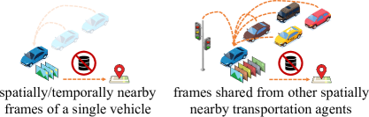
Figure 1: Multi-view camera pose regression with neighboring information, without the need for any database.

The pioneering work PoseNet (Kendall, Grimes, and Cipolla 2015) uses a convolutional neural network (CNN) to extract features from a single image as vector embeddings, and the embeddings are directly regressed to the 6-DoF poses. To further improve the regression performance in driving scenarios, multi-view-based models extend the input from a single image to multi-view images. MapNet (Brahmbhatt et al. 2018) leverages pre-computed visual odometry to post-process the output pose trajectory. GNNMapNet (Xue et al. 2020) integrates a graph neural network (GNN) into CNN to make image nodes interact with neighbors.

The above-mentioned multi-view-based models show promising performance in benign driving environments. To operate well in challenging environments, the model must be robust to environmental perturbations (e.g., changing seasons, weather, illumination, and unstable objects), and effectively leverage neighboring information from spatially or temporally nearby frames of a single vehicle or multi-view images shared from other spatially nearby agents (e.g., using V2X communication) as shown in Fig. 1. Images sharing such neighboring information are said to be covisible.

Recently, neural Ordinary Differential Equations (ODEs) (Chen et al. 2018) and Partial Differential Equations (PDEs) (Chamberlain et al. 2021b, a) have demonstrated their robustness against input perturbations (Yan et al. 2018; Kang et al. 2021). Moreover, GNNs can effectively aggregate neighborhood information. We thus propose RobustLoc that not only explores the relations between graph neighbors but also utilizes neural differential equations to improve robustness. We test our new multi-view-based model on three challenging autonomous driving datasets and verify that it outperforms existing state-of-the-art (SOTA) CPR methods.

Our main contributions are summarized as follows:

1. We represent the features extracted from a CNN in a graph and apply graph neural diffusion layers at each stage. I.e., we design feature diffusion blocks at both the feature map extraction and vector embedding stages to achieve robust feature representations. Each diffusion block consists of not only cross-diffusion from node to node in a graph but also self-diffusion within each node. We also propose multi-level training with the branched decoder to better regress the target poses.

2. We conduct experiments in both ideal and challenging noisy autonomous driving datasets to demonstrate the robustness of our proposed method. The experiments verify that our method achieves better performance than the current SOTA CPR methods.

3. We conduct extensive ablation studies to provide insights into the effectiveness of our design.

Related Work

Camera Pose Regression

Given the query images, CPR models directly regress the camera poses of these images without the need for a database. Thus, it does not depend on the scale of the database, which is definitely a born gift compared with those database methods.
PoseNet (Kendall, Grimes, and Cipolla 2015) and GeoPoseNet (Kendall and Cipolla 2017) propose the simultaneous learning for location and orientation by integrating balance parameters. MapNet (Brahmbhatt et al. 2018) uses visual odometry to serve as the post-processing technique to optimize the regressed poses. LsG (Xue et al. 2019) and LSTM-PoseNet (Walch et al. 2017) integrates the sequential information by fusing PoseNet and LSTM. AD-PoseNet and AD-MapNet (Huang et al. 2019) leverages the semantic masks to drop out the dynamic area in the image. AtLoc (Wang et al. 2020) introduces the global attention to guide the network to learn better representation. GNNMapNet (Xue et al. 2020) expands the feature exploration from a single image to multi-view images using GNN. IRPNet (Shavit and Ferens 2021) proposes to use two branches to regress translation and orientation respectively. Coordinet (Moreau et al. 2022) uses the coordconv (Liu et al. 2018) and weighted average pooling (Hu, Wang, and Lin 2017) to capture spatial relations. There are also some models focusing on LiDAR-based pose regression including PointLoc(Wang et al. 2021) and HypLiLoc(Wang et al. 2023).

Neural Differential Equations and Robustness

The dynamics of a system are usually described by ordinary or partial differential equations. The paper (Chen et al. 2018) first proposes trainable neural ODEs by parameterizing the continuous dynamics of hidden units. The hidden state of the ODE network is modeled as:

$$\frac{\mathrm{d}{\bm{y}(t)}}{\mathrm{d}{t}}=f_{\theta}(\bm{y}(t))$$ (1)

where $\bm{y}(t)$ denotes the latent state of the trainable network $f_{\theta}$ that is parameterized by weights $\theta$. Recent studies (Yan et al. 2018; Kang et al. 2021) have demonstrated that neural ODEs are intrinsically more robust against input perturbations compared to vanilla CNNs.

In addition, neural PDEs (Chamberlain et al. 2021b, a) have been proposed and applied to GNN, where the diffusion process is modeled on the graph. Furthermore, the stability of the heat semigroup and the heat kernel under perturbations of the Laplace operator (i.e., local perturbation of the manifold) is studied (Song et al. 2022).

Proposed Model

In this section, we provide a detailed description of our proposed CPR approach. We assume that the input is a set of images $\{\bm{I}_{i}\}_{i\in[N]}$ that may be covisible (see Fig. 1). Our objective is to perform CPR on the input images.

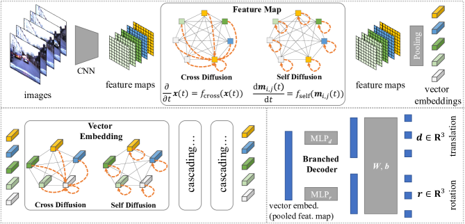
Figure 2: The main architecture of RobustLoc. Feature diffusion is performed at both the feature map stage and the vector embedding stage. The branched decoder regresses the 6-DoF poses based on the vector embeddings or the pooled feature maps. The details for multi-layer decoding are shown in Fig. 3.

RobustLoc Overview

We first summarize our multi-view CPR pipeline, which can be decomposed into three different stages, as follows (see Fig. 2 and Fig. 3):

1. Given $N$ neighboring images, a CNN extracts the feature maps of all these images. Our proposed feature map diffusion block then performs cross-self diffusion on the feature maps.

2. After feature map diffusion, a global average pooling module aggregates the feature maps as vector embeddings, which contain global representations of these images. Similarly, those vector embeddings are then diffused by cascaded diffusion blocks.

3. Based on the vector embeddings, the branched decoder module regresses the output camera poses. During training, decoding is performed on multiple levels to provide better feature constraints.

Neural Diffusion for Feature Maps

The input images $\{\bm{I}_{i}\}_{i\in[N]}$ are passed through a CNN to obtain the feature maps $\{\bm{m}_{i}\in\mathbb{R}^{H\times W\times C}\}_{i\in[N]}$. Here, $C$ is the channel dimension, while $H$ and $W$ are the dimensions of a feature map. For each feature map $\bm{m}_{i}$, we denote its $j$-th element as $\bm{m}_{i,j}\in\mathbb{R}^{C},j\in[HW]$. We next describe the feature map diffusion block, where we perform cross-diffusion from node to node in a graph, and self-diffusion within each node. The two diffusion processes update the feature map by leveraging the neighboring information or only using each node’s individual information, respectively.

Cross-Diffusion Dynamics.

To support the cross-diffusion over feature maps, we formulate the first graph in our pipeline as:

$$\mathcal{G}^{\mathrm{feat}}=(\mathcal{V}^{\mathrm{feat}},\mathcal{E}^{\mathrm{feat}}),$$ (2)

where the node set $\mathcal{V}^{\mathrm{\mathrm{feat}}}=\{\bm{m}_{i,j}\}_{(i,j)\in[N]\times[HW]}$ contains element-wise features $\bm{m}_{i,j}$ and the edge set $\mathcal{E}^{\mathrm{\mathrm{feat}}}$ is defined as the complete graph edges associated with attention weights as discussed below. And the complete graph architecture is demonstrated to be an effective design shown in Table 5.

To achieve robust feature interaction, we next define the cross-diffusion process as:

$$\frac{\partial}{\partial t}\bm{x}(t) =f_{\mathrm{cross}}(\bm{x}(t)),$$ (3)

where $f_{\mathrm{cross}}(\bm{x}(t))$ is a neural network and can be approximately viewed as a neural PDE with the partial differential operations over a manifold space replaced by the attention modules that we will introduce later. We denote the input to the feature map diffusion module as the initial state at $t=t_{0}$ as $\bm{x}(t_{0})=\left\{\bm{m}_{i,j}\right\}_{(i,j)\in[N]\times[HW]}$, where $\bm{x}(t)=\left\{\bm{m}_{i,j}(t)\right\}_{(i,j)\in[N]\times[HW]}$ denotes the hidden state of the diffusion. The diffusion process is known to have robustness against local perturbations of the manifold (Chen et al. 1998) where the local perturbations in our CPR task include challenging weather conditions, dynamic street objects, and unexpected image noise. Therefore, we expect our module 3 is simultaneously capable of leveraging the neighboring image information and holding robustness against local perturbations.

We next introduce the computation of attention weights in $f_{\mathrm{cross}}(\bm{x}(t))$ for node features at time $t$. We first generate the embedding of each node using multi-head fully connected (FC) layers with learnable parameter matrix $\bm{W}_{k}$ and bias $\bm{b}_{k}$ at each head $k=[K]$, where $K$ is the number of heads. The output at each head $k$ can be written as:

$$\bm{m}_{i,j;k}^{\mathrm{FC}}(t)=\bm{W}_{k}\bm{m}_{i,j}(t)+\bm{b}_{k}.$$ (4)

The attention weights are then generated by computing the dot product among all the neighboring nodes using the features $\bigl{\{}\bm{m}_{i,j;k}^{\mathrm{FC}}(t)\bigr{\}}_{(i,j)\in[N]\times[HW]}$. We have

$$\{a_{(i,j),(i^{\prime},j^{\prime});k}(t)\}_{(i^{\prime},j^{\prime})\in\mathcal{N}_{i,j}}$$

$$=\mathrm{Softmax}_{(i^{\prime},j^{\prime})\in\mathcal{N}(i,j)}(\bm{m}_{i,j;k}^{\mathrm{FC}}(t)\cdot\bm{m}_{i^{\prime},j^{\prime};k}^{\mathrm{FC}}(t)),$$ (5)

where $\mathcal{N}_{i,j}$ denotes the set of neighbors of node $\bm{m}_{i,j}$. Let

$$\bm{m}_{i,j;k}^{\mathrm{weighted}}(t)=\sum_{(i^{\prime},j^{\prime})\in\mathcal{N}_{i,j}}a_{(i,j),(i^{\prime},j^{\prime});k}(t)\bm{m}_{i^{\prime},j^{\prime};k}^{\mathrm{FC}}(t).$$ (6)

Finally, the updated node features are obtained by concatenating the weighted node features from all heads as

$$f_{\mathrm{cross}}(\bm{x}(t))=\left\{\operatorname*{\scalerel*{\parallel}{\sum}}_{k\in[K]}(\bm{m}_{i,j;k}^{\mathrm{weighted}}(t))\right\}_{(i,j)\in[N]\times[HW]}.$$ (7)

Based on the above pipeline, the output of the cross-diffusion at time $t=t_{1}$ can be obtained as:

$$\bm{x}(t_{1})=F_{\mathrm{cross}}(\bm{x}(t_{0})),$$ (8)

where $F_{\mathrm{cross}}(\cdot)$ denotes the solution of 3 integrated from $t=t_{0}$ to $t=t_{1}$.

Self-Diffusion Dynamics.

In the next step, we update each node feature independently. The node-wise feature update can be regarded as a rewiring of the complete graph to an edgeless graph, and the node-wise feature update is described as:

$$\frac{\mathrm{d}{\bm{m}_{i,j}(t)}}{\mathrm{d}{t}}=f_{\mathrm{self}}(\bm{m}_{i,j}(t))=\mathrm{MLP}(\bm{m}_{i,j}(t)).$$ (9)

And the output of self-diffusion can be obtained as:

$$\bm{m}_{i,j}(t_{2})=F_{\mathrm{self}}(\bm{m}_{i,j}(t_{1})).$$ (10)

where $F_{\mathrm{self}}(\cdot)$ denotes the solution of 9 integrated from $t=t_{1}$ to $t=t_{2}$. As neural ODEs are robust against input perturbations (Yan et al. 2018; Kang et al. 2021), we expect the updating of each node feature according to the self-diffusion 9 to be robust against perturbations like challenging weather conditions, dynamic street objects, and image noise.

Vector Embeddings and Diffusion

After the feature map neural diffusion, we feed the updated feature maps into a global average pooling module to generate the vector embeddings $\{\bm{h}_{i}\in\mathbb{R}^{C}\}_{i\in[N]}$, where

$$\bm{h}_{i}=\mathrm{Pooling}(\bm{m}_{i}).$$ (11)

Each vector embedding contains rich global representations for the input image together with the information diffused from the neighboring images. To enable diffusion for the global information, we propose to design the vector embedding graph as:

$$\mathcal{G}^{\mathrm{vect}}=(\mathcal{V}^{\mathrm{vect}},\mathcal{E}^{\mathrm{vect}}),$$ (12)

where the node set $\mathcal{V}^{\mathrm{vect}}=\{\bm{h}_{i}\}_{i\in[N]}$ contains image vector embeddings $\bm{h}_{i}$ and the edge set $\mathcal{E}^{\mathrm{vect}}$ is also defined to be the complete graph. Based on this graph $\mathcal{G}^{\mathrm{vect}}$, we construct the cascaded diffusion blocks, to perform global information diffusion. Within the cascaded blocks, each basic diffusion block consists of two diffusion layers: a cross-diffusion layer and a self-diffusion layer, similar to the two diffusion schemes introduced at the feature map diffusion phase.

Pose Decoding

In this subsection, we explain the pose decoding operations.

Branched Pose Decoder.

Each camera pose $\bm{p}=\{\bm{d},\bm{r}\}\in\mathbb{R}^{6}$, consists of a 3-dimensional translation $\bm{d}\in\mathbb{R}^{3}$ and a 3-dimensional rotation $\bm{r}\in\mathbb{R}^{3}$. Thus CPR can be viewed as a multi-task learning problem. However, since the translation and rotation elements of $\bm{p}$ do not scale compatibly, the regression converges in different basins. To deal with it, previous methods consider regression for translation and rotation respectively and demonstrate it is an effective way to improve performance (Shavit and Ferens 2021). In our paper, we also follow this insight to design the decoder.

Firstly, the feature embeddings $\{\bm{h}_{\bm{d}},\bm{h}_{\bm{r}}\}$ for translation and rotation are extracted from the feature embedding $\bm{h}$ using different non-linear MLP layers as:

$$\bm{h}_{\bm{d}}=\mathrm{MLP}_{\bm{d}}(\bm{h}),$$ (13)

$$\bm{h}_{\bm{r}}=\mathrm{MLP}_{\bm{r}}(\bm{h}),$$ (14)

Thus, the features of translation and rotation are decoupled. Next in the second stage, the pose output can be regressed as:

$$\bm{p}=\bm{W}(\bm{h}_{\bm{d}}\operatorname*{\scalerel*{\parallel}{\sum}}\bm{h}_{\bm{r}})+\bm{b}$$ (15)

where $\bm{W},\bm{b}$ are learnable parameters. During training, we compute the regression loss of decoded poses from multiple levels, which we will introduce below. During inference, we use the decoded pose from the last layer as the final output pose.

Multi-level Pose Decoding Graph.

To better regularize the whole regression pipeline, we propose to leverage the feature maps at multiple levels. As shown in Fig. 3, at the vector embedding stage, we use the vector embeddings to regress the poses, while at the feature map stage, we use the feature maps. Denoting the feature maps at layer $l$ as $\{\bm{m}_{i}^{l}\in\mathbb{R}^{H\times W\times C}\}_{i\in[N]}$, the pose decoding graph at layer $l$ can be formulated as:

$$\mathcal{G}^{\mathrm{pose},l}=(\mathcal{V}^{\mathrm{pose},l},\mathcal{E}^{\mathrm{pose},l}),$$ (16)

where edge set $\mathcal{E}^{\mathrm{pose},l}$ is defined to be connected with two spatially adjacent nodes which can be viewed as the odometry connection, while the node set $\mathcal{V}^{\mathrm{pose},l}$ is defined depending on layers since the information used to regress poses is different:

$$\mathcal{V}^{\mathrm{pose},l}=\left\{\begin{array}[]{ll}\{\bm{h}_{i}\}_{i\in[N]}&\text{if}\ l=L,\\ \{\bm{m}_{i}^{l}\}_{i\in[N]}&\text{otherwise},\\ \end{array}\right.$$ (19)

where $L$ represents the last layer in our network.

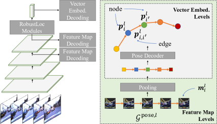
Figure 3: Multi-level pose decoding. Decoding can be directly applied to vector embeddings. Feature maps are first pooled and then decoded.

At the last layer where there are vector embeddings, we can directly apply the pose decoder to generate absolute pose messages. By contrast, at feature map layers, we first apply a global average pooling module on the feature maps to formulate feature vectors, and pose messages can be obtained using the pose decoder:

$$\bm{p}^{l}_{i}=\left\{\begin{array}[]{l l}f_{\mathrm{decoder}}^{l}(\bm{h}^{l}_{i})&\text{if}\ l=L,\\ f_{\mathrm{decoder}}^{l}(\mathrm{Pooling}(\bm{m}^{l}_{i}))&\text{otherwise}.\\ \end{array}\right.$$ (22)

where $f_{\mathrm{decoder}}^{l}(\cdot)$ is the pose decoder at layer $l$. Using the simplified relative pose computation technique in (Wang et al. 2020), the relative pose messages $\bm{p}^{l}_{i,i^{\prime}}$ at layer $l$ can be generated as:

$$\bm{p}^{l}_{i,i^{\prime}}=\bm{p}^{l}_{i^{\prime}}-\bm{p}^{l}_{i}.$$ (23)

By leveraging multi-layer information, we expect not only the last layer but also the preceding middle-level layers can directly learn the implicit relation between images and poses, which helps to improve the robustness against perturbations.

	Model	Loop (cross-day)		Loop (within-day)		Full
		Mean	Median	Mean	Median	Mean	Median
+ Extra Data	GNNMapNet + post.	7.96 / 2.56	-	-	-	17.35 / 3.47	-
	ADPoseNet	-	-	-	6.40 / 3.09	-	33.82 / 6.77
	ADMapNet	-	-	-	6.45 / 2.98	-	19.18 / 4.60
	MapNet+	8.17 / 2.62	-	-	-	30.3 / 7.8
	MapNet+ + post.	6.73 / 2.23	-	-	-	29.5 / 7.8	-
CPR Only	GeoPoseNet	27.05 / 18.54	6.34 / 2.06	-	-	125.6 / 27.1	107.6 / 22.5
	MapNet	9.30 / 3.71	5.35 / 1.61	-	-	41.4 / 12.5	17.94 / 6.68
	LsG	9.08 / 3.43	-	-	-	31.65 / 4.51	-
	AtLoc	8.74 / 4.63	5.37 / 2.12	-	-	29.6 / 12.4	11.1 / 5.28
	AtLoc+	7.53 / 3.61	4.06 / 1.98	-	-	21.0 / 6.15	6.40 / 1.50
	CoordiNet	-	-	4.06 / 1.44	2.42 / 0.88	14.96 / 5.74	3.55 / 1.14
	RobustLoc (ours)	4.68 / 2.67	3.70 / 1.50	2.49 / 1.40	1.97 / 0.84	9.37 / 2.47	5.93 / 1.06

Table 1: Median and mean translation/rotation estimation error (m/^∘) on the Oxford RobotCar dataset. The best and the second-best results in each metric are highlighted with bold and underline respectively. “-” denotes no data provided.

Loss Function

Following the approach in (Wang et al. 2020), we use a weighted balance loss for translation and rotation predictions. For the input image $I_{i}$, we denote the translation and rotation targets as $\bm{d}_{i}^{*}\in\mathbb{R}^{3}$ and $\bm{r}_{i}^{*}\in\mathbb{R}^{3}$ respectively. Then the absolute pose loss term $\mathcal{L}^{l}_{i}$ and the relative pose loss term $\mathcal{L}^{l}_{i,i^{{}^{\prime}}}$ at decoding layer $l$ are computed as:

$$\begin{multlined}\mathcal{L}^{l}_{i}=\lVert\bm{d}_{i}^{l}-\bm{d}_{i}^{*}\rVert\exp(-\alpha)+\alpha\\ +\lVert\bm{r}_{i}^{l}-\bm{r}_{i}^{*}\rVert\exp(-\beta)+\beta,\end{multlined}\mathcal{L}^{l}_{i}=\lVert\bm{d}_{i}^{l}-\bm{d}_{i}^{*}\rVert\exp(-\alpha)+\alpha\\ +\lVert\bm{r}_{i}^{l}-\bm{r}_{i}^{*}\rVert\exp(-\beta)+\beta,$$ (26)

$$\begin{multlined}\mathcal{L}^{l}_{i,i^{{}^{\prime}}}=\lVert\bm{d}_{i,i^{{}^{\prime}}}^{l}-\bm{d}_{i,i^{{}^{\prime}}}^{*}\rVert\exp(-\gamma)+\gamma\\ +\lVert\bm{r}_{i,i^{{}^{\prime}}}^{l}-\bm{r}_{i,i^{{}^{\prime}}}^{*}\rVert\exp(-\lambda)+\lambda\end{multlined}\mathcal{L}^{l}_{i,i^{{}^{\prime}}}=\lVert\bm{d}_{i,i^{{}^{\prime}}}^{l}-\bm{d}_{i,i^{{}^{\prime}}}^{*}\rVert\exp(-\gamma)+\gamma\\ +\lVert\bm{r}_{i,i^{{}^{\prime}}}^{l}-\bm{r}_{i,i^{{}^{\prime}}}^{*}\rVert\exp(-\lambda)+\lambda,$$ (29)

where $\bm{d}_{i}^{l},\bm{r}_{i}^{l},\bm{d}_{i,i^{{}^{\prime}}}^{l},\bm{r}_{i,i^{{}^{\prime}}}^{l}$ are outputs at layer $l$, while $\alpha,\beta,\gamma,\lambda$ are all learnable parameters. Finally, the overall loss function can be obtained as:

$$\mathcal{L}=\sum_{l\in\{3,4,L\}}\sum_{i\in[N],i^{{}^{\prime}}\in\mathcal{N}^{l}_{i}}\mathcal{L}^{l}_{i}+\mathcal{L}^{l}_{i,i^{{}^{\prime}}},$$ (30)

where $\mathcal{N}^{l}_{i}$ is the neighborhood of node $i$ in $\mathcal{G}^{\mathrm{pose},l}$. We use the logarithmic form of the quaternion to represent rotation $\bm{r}$ as:

$$\bm{r}=\log\bm{q}=\left\{\begin{array}[]{ll}\frac{(\bm{q}_{2},\bm{q}_{3},\bm{q}_{4})}{\lVert(\bm{q}_{2},\bm{q}_{3},\bm{q}_{4})\rVert}\cos^{-1}\bm{q}_{1}&\ \text{if}\ \lVert(\bm{q}_{2},\bm{q}_{3},\bm{q}_{4})\rVert\not=0,\\ 0&\ \text{otherwise},\end{array}\right.$$ (33)

where $\bm{q}=(\bm{q}_{1},\bm{q}_{2},\bm{q}_{3},\bm{q}_{4})\in\mathbb{R}^{4}$ represents a quaternion.

Experiments

In this section, we first evaluate our proposed model on three large autonomous driving datasets. We next present an ablation study to demonstrate the effectiveness of our model design.

Datasets and Implemention Details

Oxford RobotCar.

The Oxford RobotCar dataset(Maddern et al. 2017) is a large autonomous driving dataset collected by a car driving along a route in Oxford, UK. It consists of two different routes: 1) Loop with a trajectory area of $8.8\times 10^{4}\mathrm{m}^{2}$ and length of $10^{3}\mathrm{m}$, and 2) Full with a trajectory area of $1.2\times 10^{6}\mathrm{m}^{2}$ and length of $9\times 10^{3}\mathrm{m}$.

4Seasons.

There are only a few existing methods designed for robust CPR in driving environments, and the experiment on the Oxford dataset is insufficient for comparison. Thus we also conduct experiments on another driving dataset to cover more driving scenarios. The 4Seasons dataset (Wenzel et al. 2020) is a comprehensive dataset for autonomous driving SLAM. It was collected in Munich, Germany, covering varying perceptual conditions. Specifically, it contains different environments including the business area, the residential area, and the town area. In addition, it consists of a wide variety of weather conditions and illuminations. In our experiments, we use 1) Business Campus (business area), 2) Neighborhood (residential area), and 3) Old Town (town area).

Perturbed RobotCar.

To further evaluate the performance under challenging environments, we inject noise into the RobotCar Loop dataset and call this the Perturbed RobotCar dataset as shown in Fig. 4. We create three scenarios: 1) Medium (with fog, snow, rain, and spatter on the lens), 2) Hard (with added Gaussian noise), and 3) Hard (+ noisy training) (i.e., training with noisy augmentation).

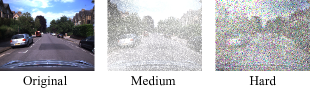
Figure 4: Visualization of the Perturbed RobotCar dataset. Medium is with fog, snow, rain, and spatter on the lens. Hard is with added Gaussian noise.

Implemention

We use ResNet34 as the backbone, which is pre-trained on the ImageNet dataset. We set the maximum number of input images as $11$. We resize the shorter side of each input image to $128$ and set the batch size to $64$. The Adam optimizer with a learning rate $2\times 10^{-4}$ and weight decay $5\times 10^{-4}$ is used to train the network. Data augmentation techniques include random cropping and color jittering. We set the integration times $t_{0}=0$, $t_{1}=1$, and $t_{2}=2$. The number of attention heads is 8. We train our network for $300$ epochs. All of the experiments are conducted on an NVIDIA A5000.

Main Results

On the Oxford RobotCar dataset, as shown in Table 1, we obtain the best performance in 10 out of 12 metrics. Using the mean error, which is easily influenced by outlier predictions, RobustLoc outperforms the baselines by a significant margin. In the most challenging route Full, to the best of our knowledge, RobustLoc is the first to achieve less than $10\mathrm{m}$ mean translation error for CPR.

The 4Seasons dataset consists of more varied driving scenes. As shown in Table 2, RobustLoc achieves the best performance in 11 out of 12 metrics. Again, using the mean error metric, RobustLoc outperforms the baselines by a significant margin.

On the Perturbed RobotCar dataset, where the images contain more challenging weather conditions and noisy perturbations, RobustLoc achieves the best in all metrics. The superiority of RobustLoc over other baselines is more obvious in Table 3.

Model	Business Campus		Neighborhood		Old Town
	Mean	Median	Mean	Median	Mean	Median
GeoPoseNet	11.04 / 5.78	5.93 / 2.03	2.87 / 1.30	1.92 / 0.88	64.81 / 6.67	15.03 / 1.57
MapNet	10.35 / 3.78	5.66 / 1.83	2.81 / 1.05	1.89 / 0.92	46.56 / 7.14	16.52 / 2.12
GNNMapNet	7.69 / 4.34	5.52 / 2.16	3.02 / 2.92	2.14 / 1.45	41.54 / 7.30	19.23 / 3.26
AtLoc	11.53 / 4.84	5.81 / 1.50	2.80 / 1.16	1.83 / 0.93	84.17 / 7.81	17.10 / 1.73
AtLoc+	13.70 / 6.41	5.58 / 1.94	2.33 / 1.39	1.61 / 0.88	68.40 / 5.51	14.52 / 1.69
IRPNet	10.95 / 5.38	5.91 / 1.82	3.17 / 2.85	1.98 / 0.90	55.86 / 6.97	17.33 / 3.11
CoordiNet	11.52 / 3.44	6.44 / 1.38	1.72 / 0.86	1.37 / 0.69	43.68 / 3.58	11.83 / 1.36
RobustLoc (ours)	4.28 / 2.04	2.55 / 1.50	1.36 / 0.83	1.00 / 0.65	21.65 / 2.41	5.52 / 1.05

Table 2: Median and mean translation/rotation estimation error (m/^∘) on the 4Seasons dataset. The best and the second-best results in each metric are highlighted with bold and underline respectively.

Model	Medium		Hard		Hard (+ noisy training)
	Mean	Median	Mean	Median	Mean	Median
GeoPoseNet	20.47 / 8.76	8.70 / 2.30	41.71 / 17.63	14.02 / 3.13	24.03 / 11.14	7.14 / 1.70
MapNet	17.93 / 7.01	6.89 / 2.00	49.36 / 20.01	18.37 / 2.58	21.22 / 8.38	6.38 / 1.97
GNNMapNet	16.17 / 7.24	8.02 / 2.35	73.97 / 35.57	61.47 / 19.73	14.55 / 7.62	6.69 / 1.57
AtLoc	19.92 / 7.25	7.26 / 1.74	52.56 / 23.46	15.01 / 3.17	23.48 / 11.43	7.42 / 2.38
AtLoc+	17.68 / 7.48	6.19 / 1.80	37.92 / 18.65	12.17 / 2.93	22.61 / 11.23	6.21 / 1.83
IRPNet	16.35 / 7.56	8.71 / 2.28	45.72 / 21.84	17.99 / 3.50	24.73 / 11.20	6.73 / 1.82
CoordiNet	17.67 / 6.66	7.63 / 1.79	44.11 / 16.42	17.21 / 2.70	24.06 / 12.27	6.25 / 1.61
RobustLoc (ours)	8.12 / 3.83	5.34 / 1.53	27.75 / 9.70	11.59 / 2.64	10.06 / 4.95	5.18 / 1.43

Table 3: Median and mean translation/rotation estimation error (m/^∘) on the Perturbed RobotCar dataset. The best and the second-best results in each metric are highlighted with bold and underline respectively. RobustLoc achieves the best in all metrics.

Analysis

Ablation Study.

We justify our design for RobustLoc by ablating each module. From Table 4, we observe that every module in our design contributes to the final improved estimation. We see that making use of neighboring information from covisible frames and learning robust feature maps contribute to more accurate CPR.

Method	Mean Error (m/∘) on Loop (c.)
base model	8.38 / 4.29
+ feature map graph	7.01 / 3.86
+ vector embedding graph	6.24 / 3.21
+ diffusion	5.53 / 2.95
+ branched decoder	5.14 / 2.79
+ multi-level decoding	4.68 / 2.67
diffusion at stage 3	5.27 / 2.90
diffusion at stage 3,4	4.86 / 3.18
diffusion at stage 4	4.68 / 2.67
multi-layer concatenation	5.80 / 3.26
more augmentation	4.68 / 2.67
less augmentation	5.32 / 3.17

Table 4: Ablation study, diffusion design, and augmentation design comparison on the Oxford RobotCar dataset.

Salience Visualization.

Salience maps shown in Fig. 5 suggest that in driving environments, RobustLoc pays more attention to relatively robust features such as the skyline and the road, similar to PixLoc (Sarlin et al. 2021). In addition, dynamic objects such as vehicles are implicitly suppressed in RobustLoc’s regression pipeline.

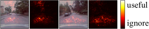
Figure 5: Robust features from RobustLoc.

Diffusion and Augmentation.

Using multi-level features is an effective method in dense prediction tasks such as depth estimation (Yan et al. 2021). To test if this holds in CPR, we use the feature maps from the lower stage 3 (see Fig. 3), which however does not lead to performance improvement shown in Table 4. We also utilize the multi-level concatenation strategy used in GNNMapNet. This does not lead to significant changes. These experiments demonstrate that CPR benefits more from high-level features with more semantic information than from low-level local texture features. Finally, we test the performance when training with less data augmentation, which leads to worse performance. This suggests that more extensive data augmentation can enhance the model robustness in challenging scenarios, which is consistent with the experimental results on the Perturbed Robotcar dataset in Table 3.

Graph Design.

We next explore the use of different graph designs for feature map diffusion and vector embedding diffusion. The grid graph stacks an image with two other spatially adjacent images as a cube, and the attention weights are formulated within the 6-neighbor area (for feature maps) or the 2-neighbor area (for vector embeddings). The self-cross graph computes attention weights first within each image and then across different images. From Table 5, we see that the complete graph has the best performance. This is because, in the complete graph, each node can interact with all other nodes, allowing the aggregation of useful information with appropriate attention weights.

Method	Mean Error (m/∘) on Full
grid graph	15.67 / 2.95
self-cross graph	15.31 / 3.28
complete graph	9.37 / 2.47
	Mean Error (∘) on Business Campus
quaternion	2.23
Lie group	2.20
rotation matrix	2.25
log (quaternion)	2.04

Table 5: Graph design comparison on the Oxford RobotCar dataset and rotation representation comparison on the 4Seasons dataset.

Rotation Representation.

We compare different representations of rotation in Table 5, where the log form of the quaternion is the optimal choice. The other three representations, including the vanilla quaternion, the Lie group, and the vanilla rotation matrix, show similar performance.

Trajectory Visualization.

We visualize the output pose trajectories as shown in Fig. 6, where a significant gap can be seen from the comparison. RobostLoc outputs more smooth and globally accurate poses compared with the previous method, which shows the effectiveness of our design.

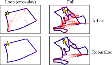
Figure 6: Trajectory visualization on the Oxford RobotCar dataset. The ground truth trajectories are shown in bold blue lines, and the estimated trajectories are shown in thin red lines. The stars mark the start of the trajectories.

Inference Speed.

We finally test the performance using a different number of input frames. The inference speed does not drop significantly when increasing the input frames. And even the slowest one (using $11$ frames) can run $50$ iterations per second and achieve real-time regression. On the other hand, more frames can bring performance improvement when the input size is small, while further increasing frame size does not bring significant change.

#frames	3	5	7	9	11
Speed (iters/s)	56	55	53	52	50
Mean Error (m)	5.28	5.09	4.96	4.68	4.72

Table 6: The performance using different numbers of frames on the Oxford RobotCar Loop (cross-day).

Conclusion

We have proposed and verified the performance of a robust CPR model RobustLoc. The model’s robustness derives from the use of information from covisible images and neural graph diffusion to aggregate neighboring information, which is present in challenging driving environments.

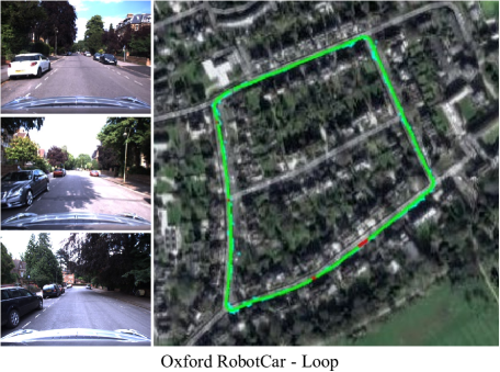
Figure 7: Visualization of the Oxford RobotCar Loop dataset. The Loop (cross-day) and the Loop (within-day) share the same images but have different data splits.

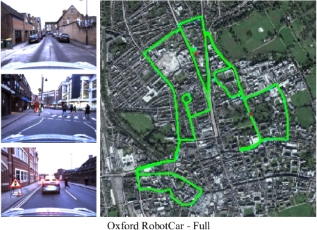
Figure 8: Visualization of the Oxford RobotCar Full dataset.

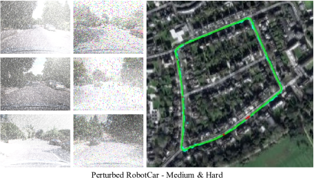
Figure 9: Visualization of the Perturbed RobotCar dataset.

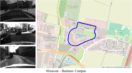
Figure 10: Visualization of the 4Seasons Business Campus dataset.

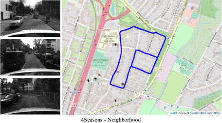
Figure 11: Visualization of the 4Seasons Neighborhood dataset.

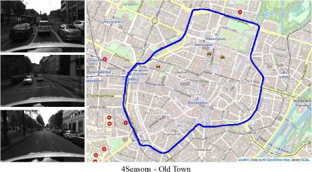
Figure 12: Visualization of the 4Seasons Old Town dataset.

Baseline Models

The baseline models in our comparison include: PoseNet, GeoPoseNet, MapNet, LsG, AtLoc/AtLoc+, GNNMapNet, ADPoseNet/ADMapNet, IRPNet, CoordiNet.

Dataset Configuration

The datasets we used in our experiments include the Oxford Robotcar dataset, the 4Seasons dataset, and the Perturbed Robotcar dataset. All of the datasets are available online at:

• https://robotcar-dataset.robots.ox.ac.uk/,

• https://vision.cs.tum.edu/data/datasets/4seasons-dataset/download.

For each dataset and each scene, we list the corresponding data split as shown in Table 7, Table 8, and Table 9.

Dataset Visualization

We visualize part of the images from the datasets we used in our experiments as shonw in Fig. 7, Fig. 8, Fig. 9, Fig. 10, Fig. 11, and Fig. 12.

Dataset	Train	Test
Loop (cross-day)	2014-06-26-08-53-56	2014-06-23-15-36-04
	2014-06-26-09-24-58	2014-06-23-15-41-25
Loop (within-day)	2014-06-26-09-24-58	2014-06-26-08-53-56
	2014-06-23-15-41-25	2014-06-23-15-36-04
Full	2014-11-28-12-07-13	2014-12-09-13-21-02
	2014-12-02-15-30-08

Table 7: The Oxford RobotCar configuration.

Dataset	Train	Test
Business Campus	2020-10-08–09-30-57	2021-02-25–14-16-43
	2021-01-07–13-12-23
Neighborhood	2020-03-26–13-32-55	2021-05-10–18-32-32
	2020-10-07–14-47-51
	2020-10-07–14-53-52
	2020-12-22–11-54-24
	2021-02-25–13-25-15
	2021-05-10–18-02-12
Old Town	2020-10-08–11-53-41	2021-02-25–12-34-08
	2021-01-07–10-49-45
	2021-05-10–21-32-00

Table 8: The 4Seasons configuration.

Dataset	Train	Test
Medium	2014-06-26-08-53-56	2014-06-23-15-36-04
	2014-06-26-09-24-58	2014-06-23-15-41-25
Hard	2014-06-26-08-53-56	2014-06-23-15-36-04
	2014-06-26-09-24-58	2014-06-23-15-41-25

Table 9: The Perturbed RobotCar configuration.

Codebase

Our codes are developed based on the following repositories:

• https://github.com/BingCS/AtLoc,

• https://github.com/psh01087/Vid-ODE.

Our codes is released at:
https://github.com/sijieaaa/RobustLoc

References

- Brahmbhatt et al. (2018) Brahmbhatt, S.; Gu, J.; Kim, K.; Hays, J.; and Kautz, J. 2018. Geometry-aware learning of maps for camera localization. In Proceedings of the IEEE conference on computer vision and pattern recognition, 2616–2625.
- Chamberlain et al. (2021a) Chamberlain, B. P.; Rowbottom, J.; Eynard, D.; Di Giovanni, F.; Xiaowen, D.; and Bronstein, M. M. 2021a. Beltrami Flow and Neural Diffusion on Graphs. In Proc. Advances Neural Inf. Process. Syst.
- Chamberlain et al. (2021b) Chamberlain, B. P.; Rowbottom, J.; Goronova, M.; Webb, S.; Rossi, E.; and Bronstein, M. M. 2021b. GRAND: Graph Neural Diffusion. In Proc. Int. Conf. Mach. Learn.
- Chen et al. (2018) Chen, R. T.; Rubanova, Y.; Bettencourt, J.; and Duvenaud, D. 2018. Neural ordinary differential equations. arXiv preprint arXiv:1806.07366.
- Chen et al. (1998) Chen, Z.-Q.; Qian, Z.; Hu, Y.; and Zheng, W. 1998. Stability and approximations of symmetric diffusion semigroups and kernels. J. functional anal., 152(1): 255–280.
- Hu, Wang, and Lin (2017) Hu, Y.; Wang, B.; and Lin, S. 2017. Fc4: Fully convolutional color constancy with confidence-weighted pooling. In Proceedings of the IEEE conference on computer vision and pattern recognition, 4085–4094.
- Huang et al. (2019) Huang, Z.; Xu, Y.; Shi, J.; Zhou, X.; Bao, H.; and Zhang, G. 2019. Prior guided dropout for robust visual localization in dynamic environments. In Proceedings of the IEEE/CVF International Conference on Computer Vision, 2791–2800.
- Kang et al. (2021) Kang, Q.; Song, Y.; Ding, Q.; and Tay, W. P. 2021. Stable neural ODE with Lyapunov-stable equilibrium points for defending against adversarial attacks. In Proc. Advances Neural Inf. Process. Syst.
- Kendall and Cipolla (2017) Kendall, A.; and Cipolla, R. 2017. Geometric loss functions for camera pose regression with deep learning. In Proceedings of the IEEE conference on computer vision and pattern recognition, 5974–5983.
- Kendall, Grimes, and Cipolla (2015) Kendall, A.; Grimes, M.; and Cipolla, R. 2015. Posenet: A convolutional network for real-time 6-dof camera relocalization. In Proceedings of the IEEE international conference on computer vision, 2938–2946.
- Liu et al. (2018) Liu, R.; Lehman, J.; Molino, P.; Petroski Such, F.; Frank, E.; Sergeev, A.; and Yosinski, J. 2018. An intriguing failing of convolutional neural networks and the coordconv solution. Advances in neural information processing systems, 31.
- Maddern et al. (2017) Maddern, W.; Pascoe, G.; Linegar, C.; and Newman, P. 2017. 1 year, 1000 km: The Oxford RobotCar dataset. The International Journal of Robotics Research, 36(1): 3–15.
- Moreau et al. (2022) Moreau, A.; Piasco, N.; Tsishkou, D.; Stanciulescu, B.; and de La Fortelle, A. 2022. CoordiNet: uncertainty-aware pose regressor for reliable vehicle localization. In Proceedings of the IEEE/CVF Winter Conference on Applications of Computer Vision, 2229–2238.
- Sarlin et al. (2021) Sarlin, P.-E.; Unagar, A.; Larsson, M.; Germain, H.; Toft, C.; Larsson, V.; Pollefeys, M.; Lepetit, V.; Hammarstrand, L.; Kahl, F.; et al. 2021. Back to the feature: Learning robust camera localization from pixels to pose. In Proceedings of the IEEE/CVF conference on computer vision and pattern recognition, 3247–3257.
- Shavit and Ferens (2021) Shavit, Y.; and Ferens, R. 2021. Do We Really Need Scene-specific Pose Encoders? In 2020 25th International Conference on Pattern Recognition (ICPR), 3186–3192. IEEE.
- Song et al. (2022) Song, Y.; Kang, Q.; Wang, S.; Zhao, K.; and Tay, W. P. 2022. On the Robustness of Graph Neural Diffusion to Topology Perturbations. In Advances in Neural Information Processing Systems (NeurIPS). New Orleans, USA.
- Walch et al. (2017) Walch, F.; Hazirbas, C.; Leal-Taixe, L.; Sattler, T.; Hilsenbeck, S.; and Cremers, D. 2017. Image-based localization using lstms for structured feature correlation. In Proceedings of the IEEE International Conference on Computer Vision, 627–637.
- Wang et al. (2020) Wang, B.; Chen, C.; Lu, C. X.; Zhao, P.; Trigoni, N.; and Markham, A. 2020. Atloc: Attention guided camera localization. In Proceedings of the AAAI Conference on Artificial Intelligence, 10393–10401.
- Wang et al. (2023) Wang, S.; Kang, Q.; She, R.; Wang, W.; Zhao, K.; Song, Y.; and Tay, W. P. 2023. HypLiLoc: Towards Effective LiDAR Pose Regression with Hyperbolic Fusion. In Proceedings of the IEEE/CVF Conference on Computer Vision and Pattern Recognition, 5176–5185.
- Wang et al. (2021) Wang, W.; Wang, B.; Zhao, P.; Chen, C.; Clark, R.; Yang, B.; Markham, A.; and Trigoni, N. 2021. Pointloc: Deep pose regressor for lidar point cloud localization. IEEE Sensors Journal, 22(1): 959–968.
- Wenzel et al. (2020) Wenzel, P.; Wang, R.; Yang, N.; Cheng, Q.; Khan, Q.; von Stumberg, L.; Zeller, N.; and Cremers, D. 2020. 4Seasons: A cross-season dataset for multi-weather SLAM in autonomous driving. In DAGM German Conference on Pattern Recognition, 404–417. Springer.
- Xue et al. (2019) Xue, F.; Wang, X.; Yan, Z.; Wang, Q.; Wang, J.; and Zha, H. 2019. Local supports global: Deep camera relocalization with sequence enhancement. In Proceedings of the IEEE/CVF International Conference on Computer Vision, 2841–2850.
- Xue et al. (2020) Xue, F.; Wu, X.; Cai, S.; and Wang, J. 2020. Learning multi-view camera relocalization with graph neural networks. In 2020 IEEE/CVF Conference on Computer Vision and Pattern Recognition (CVPR), 11372–11381. IEEE.
- Yan et al. (2018) Yan, H.; Du, J.; Tan, V. Y.; and Feng, J. 2018. On robustness of neural ordinary differential equations. In Proc. Advances Neural Inf. Process. Syst., 1–13.
- Yan et al. (2021) Yan, J.; Zhao, H.; Bu, P.; and Jin, Y. 2021. Channel-Wise Attention-Based Network for Self-Supervised Monocular Depth Estimation. In 2021 International Conference on 3D Vision (3DV), 464–473. IEEE.