DynIBaR: Neural Dynamic Image-Based Rendering

Abstract

We address the problem of synthesizing novel views from a monocular video depicting a complex dynamic scene. State-of-the-art methods based on temporally varying Neural Radiance Fields (aka dynamic NeRFs) have shown impressive results on this task. However, for long videos with complex object motions and uncontrolled camera trajectories, these methods can produce blurry or inaccurate renderings, hampering their use in real-world applications. Instead of encoding the entire dynamic scene within the weights of MLPs, we present a new approach that addresses these limitations by adopting a volumetric image-based rendering framework that synthesizes new viewpoints by aggregating features from nearby views in a scene motion–aware manner. Our system retains the advantages of prior methods in its ability to model complex scenes and view-dependent effects, but also enables synthesizing photo-realistic novel views from long videos featuring complex scene dynamics with unconstrained camera trajectories. We demonstrate significant improvements over state-of-the-art methods on dynamic scene datasets, and also apply our approach to in-the-wild videos with challenging camera and object motion, where prior methods fail to produce high-quality renderings.

Figure 1: Recent methods for synthesizing novel views from monocular videos of dynamic scenes–like HyperNeRF [50] and NSFF [35]–struggle to render high-quality views from long videos featuring complex camera and scene motion. We present a new approach that addresses these limitations, illustrated above via an application to $6$DoF video stabilization, where we apply our approach and prior methods on a 30-second, shaky video clip, and compare novel views rendered along a smoothed camera path (left). On a dynamic scenes dataset (right) [75], our approach significantly improves rendering fidelity, as indicated by synthesized images and LPIPS errors computed on pixels corresponding to moving objects (yellow numbers). Please see the supplementary video for full results.

1 Introduction

Computer vision methods can now produce free-viewpoint renderings of static 3D scenes with spectacular quality. What about moving scenes, like those featuring people or pets? Novel view synthesis from a monocular video of a dynamic scene is a much more challenging dynamic scene reconstruction problem. Recent work has made progress towards synthesizing novel views in both space and time, thanks to new time-varying neural volumetric representations like HyperNeRF [50] and Neural Scene Flow Fields (NSFF) [35], which encode spatiotemporally varying scene content volumetrically within a coordinate-based multi-layer perceptron (MLP).

However, these dynamic NeRF methods have limitations that prevent their application to casual, in-the-wild videos. Local scene flow–based methods like NSFF struggle to scale to longer input videos captured with unconstrained camera motions: the NSFF paper only claims good performance for 1-second, forward-facing videos [35]. Methods like HyperNeRF that construct a canonical model are mostly constrained to object-centric scenes with controlled camera paths, and can fail on scenes with complex object motion.

In this work, we present a new approach that is scalable to dynamic videos captured with 1) long time duration, 2) unbounded scenes, 3) uncontrolled camera trajectories, and 4) fast and complex object motion. Our approach retains the advantages of volumetric scene representations that can model intricate scene geometry with view-dependent effects, while significantly improving rendering fidelity for both static and dynamic scene content compared to recent methods [35, 50], as illustrated in Fig. 1.

We take inspiration from recent methods for rendering static scenes that synthesize novel images by aggregating local image features from nearby views along epipolar lines [70, 64, 39]. However, scenes that are in motion violate the epipolar constraints assumed by those methods. We instead propose to aggregate multi-view image features in scene motion–adjusted ray space, which allows us to correctly reason about spatio-temporally varying geometry and appearance.

We also encountered many efficiency and robustness challenges in scaling up aggregation-based methods to dynamic scenes. To efficiently model scene motion across multiple views, we model this motion using motion trajectory fields that span multiple frames, represented with learned basis functions. Furthermore, to achieve temporal coherence in our dynamic scene reconstruction, we introduce a new temporal photometric loss that operates in motion-adjusted ray space. Finally, to improve the quality of novel views, we propose to factor the scene into static and dynamic components through a new IBR-based motion segmentation technique within a Bayesian learning framework.

On two dynamic scene benchmarks, we show that our approach can render highly detailed scene content and significantly improves upon the state-of-the-art, leading to an average reduction in LPIPS errors by over 50% both across entire scenes, as well as on regions corresponding to dynamic objects. We also show that our method can be applied to in-the-wild videos with long duration, complex scene motion, and uncontrolled camera trajectories, where prior state-of-the-art methods fail to produce high quality renderings. We hope that our work advances the applicability of dynamic view synthesis methods to real-world videos.

2 Related Work

Novel view synthesis.

Classic image-based rendering (IBR) methods synthesize novel views by integrating pixel information from input images [58], and can be categorized according to their dependence on explicit geometry. Light field or lumigraph rendering methods [32, 21, 9, 26] generate new views by filtering and interpolating sampled rays, without use of explicit geometric models. To handle sparser input views, many approaches [14, 7, 30, 24, 52, 23, 18, 54, 55, 26] leverage pre-computed proxy geometry such as depth maps or meshes to render novel views.

Recently, neural representations have demonstrated high-quality novel view synthesis [81, 62, 12, 17, 59, 61, 60, 40, 46, 38, 48, 72]. In particular, Neural Radiance Fields (NeRF) [46] achieves an unprecedented level of fidelity by encoding continuous scene radiance fields within multi-layer perceptrons (MLPs). Among all methods building on NeRF, IBRNet [70] is the most relevant to our work. IBRNet combines classical IBR techniques with volume rendering to produce a generalized IBR module that can render high-quality views without per-scene optimization. Our work extends this kind of volumetric IBR framework designed for static scenes [70, 64, 11] to more challenging dynamic scenes. Note that our focus is on synthesizing higher-quality novel views for long videos with complex camera and object motion, rather than on generalization across scenes.

Dynamic scene view synthesis.

Our work is related to geometric reconstruction of dynamic scenes from RGBD [15, 47, 25, 83, 5, 68] or monocular videos [80, 44, 31, 78]. However, depth- or mesh-based representations struggle to model complex geometry and view-dependent effects.

Most prior work on novel view synthesis for dynamic scenes requires multiple synchronized input videos [27, 1, 3, 63, 82, 33, 6, 76, 69], limiting their real-world applicability. Some methods [8, 13, 22, 51, 71] use domain knowledge such as template models to achieve high-quality results, but are restricted to specific categories [41, 56]. More recently, many works propose to synthesize novel views of dynamic scenes from a single camera. Yoon et al. [75] render novel views through explicit warping using depth maps obtained via single-view depth and multi-view stereo. However, this method fails to model complex scene geometry and to fill in realistic and consistent content at disocclusions. With advances in neural rendering, NeRF-based dynamic view synthesis methods have shown state-of-the-art results [74, 66, 35, 53, 16]. Some approaches, such as Nerfies [49] and HyperNeRF [50], represent scenes using a deformation field mapping each local observation to a canonical scene representation. These deformations are conditioned on time [53] or a per-frame latent code [66, 49, 50], and are parameterized as translations [53, 66] or rigid body motion fields [49, 50]. These methods can handle long videos, but are mostly limited to object-centric scenes with relatively small object motion and controlled camera paths. Other methods represent scenes as time-varying NeRFs [35, 74, 67, 19, 20]. In particular, NSFF uses neural scene flow fields that can capture fast and complex 3D scene motion for in-the-wild videos [35]. However, this method only works well for short (1-2 second), forward-facing videos.

3 Dynamic Image-Based Rendering

Given a monocular video of a dynamic scene with frames $(I_{1},I_{2},\ldots,I_{N})$ and known camera parameters $(\mathbf{P}_{1},\mathbf{P}_{2},\ldots,\mathbf{P}_{N})$, our goal is to synthesize a novel viewpoint at any desired time within the video. Like many other approaches, we train per-video, first optimizing a model to reconstruct the input frames, then using this model to render novel views.

Rather than encoding 3D color and density directly in the weights of an MLP as in recent dynamic NeRF methods, we integrate classical IBR ideas into a volumetric rendering framework. Compared to explicit surfaces, volumetric representations can more readily model complex scene geometry with view-dependent effects.

The following sections introduce our methods for scene-motion-adjusted multi-view feature aggregation (Sec. 3.1), and enforcing temporal consistency via cross-time rendering in motion-adjusted ray space (Sec. 3.2). Our full system combines a static model and a dynamic model to produce a color at each pixel. Accurate scene factorization is achieved via segmentation masks derived from a separately trained motion segmentation module within a Bayesian learning framework (Sec. 3.3).

3.1 Motion-adjusted feature aggregation

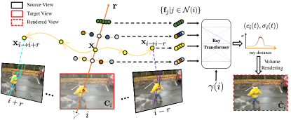
Figure 2: Rendering via motion-adjusted multi-view feature aggregation. Given a sampled location $\mathbf{x}$ at time $i$ along a target ray $\mathbf{r}$, we estimate its motion trajectory, which determines the 3D correspondence of $\mathbf{x}$ at nearby time $j\in\mathcal{N}(i)$, denoted $\mathbf{x}_{{i\rightarrow j}}$. Each warped point is then projected into its corresponding source view. Image features ${\mathbf{f}}_{j}$ extracted along the projected curves are aggregated and fed to the ray transformer with time embedding $\gamma(i)$, producing per-sample color and density $(\mathbf{c}_{i},\sigma_{i})$. The final pixel color $\hat{\mathbf{C}}_{i}$ is then synthesized by volume rendering $(\mathbf{c}_{i},\sigma_{i})$ along $\mathbf{r}$.

We synthesize new views by aggregating features extracted from temporally nearby source views. To render an image at time $i$, we first identify source views $I_{j}$ within a temporal radius $r$ frames of $i$, $j\in\mathcal{N}(i)=[i-r,i+r]$. For each source view, we extract a 2D feature map $F_{i}$ through a shared convolutional encoder network to form an input tuple $\{I_{j},\mathbf{P}_{j},F_{j}\}$.

To predict the color and density of each point sampled along a target ray $\mathbf{r}$, we must aggregate source view features while accounting for scene motion. For a static scene, points along a target ray will lie along a corresponding epipolar line in a neighboring source view, hence we can aggregate potential correspondences by simply sampling along neighboring epipolar lines [70, 64]. However, moving scene elements violate epipolar constraints, leading to inconsistent feature aggregation if motion is not accounted for. Hence, we perform motion-adjusted feature aggregation, as shown in Fig. 3. To determine correspondence in dynamic scenes, one straightforward idea is to estimate a scene flow field via an MLP [35] to determine a given point’s motion-adjusted 3D location at a nearby time. However, this strategy is computational infeasible in a volumetric IBR framework due to recursive unrolling of the MLPs.

Motion trajectory fields. Instead, we represent scene motion using motion trajectory fields described in terms of learned basis functions. For a given 3D point $\mathbf{x}$ along target ray $\mathbf{r}$ at time $i$, we encode its trajectory coefficients with an MLP $G_{\text{MT}}$:

$$\{\phi^{l}_{i}(\mathbf{x})\}_{l=1}^{L}=G_{\text{MT}}\left(\gamma(\mathbf{x}),\gamma(i)\right),$$ (1)

where $\phi^{l}_{i}\in\mathcal{R}^{3}$ are basis coefficients (with separate coefficients for $x$, $y$, and $z$, using the motion basis described below) and $\gamma$ denotes positional encoding. We choose $L=6$ bases and 16 linearly increasing frequencies for the encoding $\gamma$, based on the assumption that scene motion tends to be low frequency [80].

We also introduce a global learnable motion basis $\{h_{i}^{l}\}^{L}_{l=1},h_{i}^{l}\in\mathcal{R}$, spanning every time step $i$ of the input video, which is optimized jointly with the MLP. The motion trajectory of $\mathbf{x}$ is then defined as $\Gamma_{\mathbf{x},i}(j)=\sum_{l=1}^{L}h^{l}_{j}\phi^{l}_{i}(\mathbf{x})$, and thus, the relative displacement between $\mathbf{x}$ and its 3D correspondence $\mathbf{x}_{i\rightarrow j}$ at time $j$ is computed as

$$\Delta_{\mathbf{x},i}(j)=\Gamma_{\mathbf{x},i}(j)-\Gamma_{\mathbf{x},i}(i).$$ (2)

With this motion trajectory representation, finding 3D correspondences for a query point $\mathbf{x}$ in neighboring views requires just a single MLP query, allowing efficient multi-view feature aggregation within our volume rendering framework. We initialize the basis $\{h_{i}^{l}\}_{l=1}^{L}$ with the DCT basis as proposed by Wang et al. [67], but fine-tune it along with other components during optimization, since we observe that a fixed DCT basis can fail to model a wide range of real-world motions (see third column of Fig. 4).

Using the estimated motion trajectory of $\mathbf{x}$ at time $i$, we denote $\mathbf{x}$’s corresponding 3D point at time $j$ as $\mathbf{x}_{i\rightarrow j}=\mathbf{x}+\Delta_{\mathbf{x},i}(j)$. We project each warped point $\mathbf{x}_{i\rightarrow j}$ into its source view $I_{j}$ using camera parameters $\mathbf{P}_{j}$, and extract color and feature vector ${\mathbf{f}}_{j}$ at the projected 2D pixel location. The resulting set of source features across neighbor views $j$ is fed to a shared MLP whose output features are aggregated through weighted average pooling [70] to produce a single feature vector at each 3D sample point along ray $\mathbf{r}$. A ray transformer network with time embedding $\gamma(i)$ then processes the sequence of aggregated features along the ray to predict per-sample colors and densities $(\mathbf{c}_{i},\sigma_{i})$ (see Fig. 2). We then use standard NeRF volume rendering [4] to obtain a final pixel color $\hat{\mathbf{C}}_{i}(\mathbf{r})$ for the ray from this sequence of colors and densities.

3.2 Cross-time rendering for temporal consistency

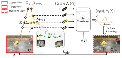
Figure 3: Temporal consistency via cross-time rendering. To enforce temporal consistency in a dynamic reconstruction, we render each frame $I_{i}$ using the scene model from a nearby time $j$, which we call cross-time rendering. A ray $\mathbf{r}$ from image $i$ is instead rendered using a curved ray $\mathbf{r}_{i\rightarrow j}$, i.e., $\mathbf{r}$ warped to time $j$. That is, having computed the motion-adjusted point $\mathbf{x}_{i\rightarrow j}=\mathbf{x}+\Delta_{\mathbf{x},i}(j)$ at nearby time $j$ from every sampled location along $\mathbf{r}$, we query $\mathbf{x}_{i\rightarrow j}$ and time $j$ via the MLP to predict its motion trajectory $\Gamma_{\mathbf{x}_{i\rightarrow j},j}$, along which we aggregate image features ${\mathbf{f}}_{k}$ extracted from source views within time $k\in\mathcal{N}(j)$. The aggregated features along $\mathbf{r}_{i\rightarrow j}$ are fed to the ray transformer with time embedding $\gamma(j)$ to produce per-sample color and density $(\mathbf{c}_{j},\sigma_{j})$ at time $j$. A pixel color $\hat{\mathbf{C}}_{j\rightarrow i}$ is computed by volume rendering $(\mathbf{c}_{j},\sigma_{j})$, and then compared to the ground truth color ${\mathbf{C}}_{i}$ to form a reconstruction loss $\mathcal{L}_{\text{pho}}$.

If we optimize our dynamic scene representation by comparing $\hat{\mathbf{C}}_{i}$ with ${\mathbf{C}}_{i}$ alone, the representation might overfit to the input images: it might perfectly reconstruct those views, but fail to render correct novel views. This can happen because the representation has the capacity to reconstruct completely separate models for each time instance, without utilizing or accurately reconstructing scene motion. Therefore, to recover a consistent scene with physically plausible motion, we enforce temporal coherence of the scene representation. One way to define temporal coherence in this context is that the scene at two neighboring times $i$ and $j$ should be consistent when taking scene motion into account[35, 19, 67].

In particular, we enforce temporal photometric consistency in our optimized representation via cross-time rendering in motion-adjusted ray space, as shown in Fig. 3. The idea is to render a view at time $i$ but via some nearby time $j$, which we refer to as cross-time rendering. For each nearby time $j\in\mathcal{N}(i)$, rather than directly using points $\mathbf{x}$ along ray $\mathbf{r}$, we consider the points $\mathbf{x}_{i\rightarrow j}$ along motion-adjusted ray $\mathbf{r}_{i\rightarrow j}$ and treat them as if they lie along a ray at time $j$.

Specifically, having computed the motion-adjusted points $\mathbf{x}_{i\rightarrow j}$, we query the MLP to predict the coefficients of new trajectories $\{\phi^{l}_{j}(\mathbf{x}_{i\rightarrow j}\}_{l=1}^{L}=G_{\text{MT}}(\mathbf{x}_{i\rightarrow j},\gamma(j))$, and use these to compute corresponding 3D points $(\mathbf{x}_{i\rightarrow j})_{j\rightarrow k}$ for images $k$ in the temporal window $\mathcal{N}(j)$, using Eq. 2. These new 3D correspondences are then used to render a pixel color exactly as described for a “straight” ray $\mathbf{r}_{i}$ in Sec. 3.1, except now along the curved, motion-adjusted ray $\mathbf{r}_{i\rightarrow j}$. That is, each point $(\mathbf{x}_{i\rightarrow j})_{j\rightarrow k}$ is projected into its source view $I_{k}$ and feature maps $F_{k}$ with camera parameters $\mathbf{P}_{k}$ to extract an RGB color and image feature ${\mathbf{f}}_{k}$, and then these features are aggregated and input to the ray transformer with the time embedding $\gamma(j)$. The result is a sequence of colors and densities $(\mathbf{c}_{j},\sigma_{j})$ along $\mathbf{r}_{i\rightarrow j}$ at time $j$, which can be composited through volume rendering to form a color $\hat{\mathbf{C}}_{j\rightarrow i}$.

We can then compare $\hat{\mathbf{C}}_{j\rightarrow i}(\mathbf{r})$ with the target pixel ${\mathbf{C}}_{i}(\mathbf{r})$ via a motion-disocclusion-aware RGB reconstruction loss:

$$\mathcal{L}_{\text{pho}}=\sum_{\mathbf{r}}\sum_{j\in\mathcal{N}(i)}\hat{\mathbf{W}}_{j\rightarrow i}(\mathbf{r})\rho({\mathbf{C}}_{i}(\mathbf{r}),\hat{\mathbf{C}}_{j\rightarrow i}(\mathbf{r})).$$ (3)

We use a generalized Charbonnier loss [10] for the RGB loss $\rho$. $\hat{\mathbf{W}}_{j\rightarrow i}(\mathbf{r})$ is a motion disocclusion weight computed by the difference of accumulated alpha weights between time $i$ and $j$ to address the motion disocclusion ambiguity described by NSFF [35] (see supplement for more details). Note that when $j=i$, there is no scene motion–induced displacement, meaning $\hat{\mathbf{C}}_{j\rightarrow i}=\hat{\mathbf{C}}_{i}$ and no disocclusion weights are involved ($\hat{\mathbf{W}}_{j\rightarrow i}=1$). We show a comparison between our method with and without enforcing temporal consistency in the first column of Fig. 4.

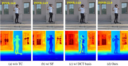
Figure 4: Qualitative ablations. From left to right, we show rendered novel views (top) and depths (bottom) from our system (a) without enforcing temporal consistency, (b) aggregating image features with scene flow fields instead of motion trajectories, (c) representing motion trajectory with a fixed DCT basis instead of a learned one, and (d) with full configuration. Simpler configurations significantly degrade rendering quality as indicated by PSNR calculated over the regions of moving objects.

3.3 Combining static and dynamic models

As observed in NSFF, synthesizing novel views using a small temporal window is insufficient to recover complete and high-quality content for static scene regions, since the contents may only be observed in spatially distant frames due to uncontrolled camera paths. Therefore, we follow the ideas of NSFF [35], and model the entire scene using two separate representations. Dynamic content $(\mathbf{c}_{i},\sigma_{i})$ is represented with a time-varying model as above (used for cross-time rendering during optimization). Static content $(\mathbf{c},\sigma)$ is represented with a time-invariant model, which renders in the same way as the time-varying model, but aggregates multi-view features without scene motion adjustment (i.e., along epipolar lines).

The dynamic and static predictions are combined and rendered to a single output color $\hat{\mathbf{C}}^{\text{full}}_{i}$ (or $\hat{\mathbf{C}}^{\text{full}}_{j\rightarrow i}$ during cross-time rendering) using the method for combining static and transient models of NeRF-W [45]. Each model’s color and density estimates can also be rendered separately, giving color $\hat{\mathbf{C}}^{\text{st}}$ for static content and $\hat{\mathbf{C}}_{i}^{\text{dy}}$ for dynamic content.

When combining the two representations, we rewrite the photometric consistency term in Eq. 3 as a loss comparing $\hat{\mathbf{C}}^{\text{full}}_{j\rightarrow i}(\mathbf{r})$ with target pixel ${\mathbf{C}}_{i}(\mathbf{r})$:

$$\mathcal{L}_{\text{pho}}=\sum_{\mathbf{r}}\sum_{j\in\mathcal{N}(i)}\hat{\mathbf{W}}_{j\rightarrow i}(\mathbf{r})\rho({\mathbf{C}}_{i}(\mathbf{r}),\hat{\mathbf{C}}^{\text{full}}_{j\rightarrow i}(\mathbf{r}))$$ (4)

Image-based motion segmentation.

In our framework, we observed that without any initialization, scene factorization tends to be dominated by either the time-invariant or the time-varying representation, a phenomena also observed in recent methods [42, 28]. To facilitate factorization, Gao$~{}\emph{et al}.\hbox{}$ [19] initialize their system using masks from semantic segmentation, relying on the assumption that all moving objects are captured by a set of candidate semantic segmentation labels, and segmentation masks are temporally accurate. However, these assumptions do not hold in many real-world scenarios, as observed by Zhang et al. [79]. Instead, we propose a new motion segmentation module that produces segmentation masks for supervising our main two-component scene representation. Our idea is inspired by the Bayesian learning techniques proposed in recent work [45, 79], but integrated into a volumetric IBR representation for dynamic videos.

In particular, before training our main two-component scene representation, we jointly train two lightweight models to obtain a motion segmentation mask $M_{i}$ for each input frame $I_{i}$. We model static scene content with an IBRNet [70] that renders a pixel color $\hat{\mathbf{B}}^{\text{st}}$ using volume rendering along each ray via feature aggregation along epipolar lines from nearby source views without considering scene motion; we model dynamic scene content with a 2D convolutional encoder-decoder network $D$, which predicts a 2D opacity map $\boldsymbol{\alpha}^{\text{dy}}_{i}$, confidence map $\boldsymbol{\beta}^{\text{dy}}_{i}$, and RGB image $\hat{\mathbf{B}}^{\text{dy}}_{i}$ from an input frame:

$$\hat{\mathbf{B}}^{\text{dy}}_{i},\boldsymbol{\alpha}^{\text{dy}}_{i},\boldsymbol{\beta}^{\text{dy}}_{i}=D(I_{i}).$$ (5)

The full reconstructed image is then composited pixelwise from the outputs of the two models:

$$\hat{\mathbf{B}}^{\text{full}}_{i}(\mathbf{r})=\boldsymbol{\alpha}^{\text{dy}}_{i}(\mathbf{r})\hat{\mathbf{B}}^{\text{dy}}_{i}(\mathbf{r})+(1-\boldsymbol{\alpha}^{\text{dy}}_{i}(\mathbf{r}))\hat{\mathbf{B}}^{\text{st}}(\mathbf{r}).$$ (6)

To segment moving objects, we assume the observed pixel color is uncertain in a heteroscedastic aleatoric manner, and model the observations in the video with a Cauchy distribution with time dependent confidence $\boldsymbol{\beta}^{\text{dy}}_{i}$. By taking the negative log-likelihood of the observations, our segmentation loss is written as a weighted reconstruction loss:

$$\mathcal{L}_{\text{seg}}=\sum_{\mathbf{r}}\log\left(\boldsymbol{\beta}^{\text{dy}}_{i}(\mathbf{r})+\frac{||\hat{\mathbf{B}}^{\text{full}}_{i}(\mathbf{r})-{\mathbf{C}}_{i}(\mathbf{r})||^{2}}{\boldsymbol{\beta}^{\text{dy}}_{i}(\mathbf{r})}\right).$$ (7)

By optimizing the two models using Eq. 7, we obtain a motion segmentation mask $M_{i}$ by thresholding $\boldsymbol{\alpha}^{\text{dy}}_{i}$ at $0.5$. We do not require an alpha regularization loss as in NeRF-W [45] to avoid degeneracies, since we naturally include such an inductive basis by excluding skip connections from network $D$, which leads $D$ to converge more slowly than the static IBR model. We show our estimated motion segmentation masks overlaid on input images in Fig. 5.

Figure 5: Motion segmentation. We show full rendering $\hat{\mathbf{B}}^{\text{full}}_{i}$ (top) and motion segmentation overlaid with rendered dynamic content $\boldsymbol{\alpha}^{\text{dy}}_{i}\odot\hat{\mathbf{B}}^{\text{dy}}_{i}$ (bottom). Our approach segments challenging dynamic elements such as the moving shadow, swing, and swaying bushes.

Supervision with segmentation masks. We initialize our main time-varying and time-invariant models with masks $M_{i}$ as in Omnimatte [43], by applying a reconstruction loss to renderings from the time-varying model in dynamic regions, and to renderings from the time-invariant model in static regions:

$$\mathcal{L}_{\text{mask}}= \sum_{\mathbf{r}}(1-M_{i})(\mathbf{r})\rho(\hat{\mathbf{C}}^{\text{st}}(\mathbf{r}),{\mathbf{C}}_{i}(\mathbf{r}))$$

$$+ \sum_{\mathbf{r}}M_{i}(\mathbf{r})\rho(\hat{\mathbf{C}}^{\text{dy}}_{i}(\mathbf{r}),{\mathbf{C}}_{i}(\mathbf{r}))$$ (8)

We perform morphological erosion and dilation on $M_{i}$ to obtain masks of dynamic and static regions respectively in order to turn off the loss near mask boundaries. We supervise the system with $\mathcal{L}_{\text{mask}}$ and decay the weights by a factor of 5 for dynamic regions every 50K optimization steps.

3.4 Regularization

As noted in prior work, monocular reconstruction of complex dynamic scenes is highly ill-posed, and using photometric consistency alone is insufficient to avoid bad local minima during optimization [35, 19]. Therefore, we adopt regularization schemes used in prior work [2, 35, 75, 73], which consist of three main parts $\mathcal{L}_{\text{reg}}=\mathcal{L}_{\text{data}}+\mathcal{L}_{\text{MT}}+\mathcal{L}_{\text{cpt}}$. $\mathcal{L}_{\text{data}}$ is a data-driven term consisting of $\ell_{1}$ monocular depth and optical flow consistency priors using the estimates from Zhang et al. [80] and RAFT [65]. $\mathcal{L}_{\text{MT}}$ is a motion trajectory regularization term that encourages estimated trajectory fields to be cycle-consistent and spatial-temporally smooth. $\mathcal{L}_{\text{cpt}}$ is a compactness prior that encourages the scene decomposition to be binary via an entropy loss, and mitigates floaters through distortion losses [2]. We refer readers to the supplement for more details.

In summary, the final combined loss used to optimize our main representation for space-time view synthesis is:

$$\mathcal{L} =\mathcal{L}_{\text{pho}}+\mathcal{L}_{\text{mask}}+\mathcal{L}_{\text{reg}}.$$ (9)

4 Implementation details

Data.

We conduct numerical evaluations on the Nvidia Dynamic Scene Dataset [75] and UCSD Dynamic Scenes Dataset [37]. Each dataset consists of eight forward-facing dynamic scenes recorded by synchronized multi-view cameras. We follow prior work [35] to derive a monocular video from each sequence, where each video contains 100$\sim$250 frames. We removed frames that lack large regions of moving objects. We follow the protocol from prior work [35] that uses held-out images per time instance for evaluation. We also tested the methods on in-the-wild monocular videos, which feature more challenging camera and object motions [20].

View selection.

For the time-varying, dynamic model we use a frame window radius of $r=3$ for all experiments. For the time-invariant model representing static scene content, we use separate strategies for the dynamic scenes benchmarks and for in-the-wild videos. For the benchmarks, where camera viewpoints are located at discrete camera rig locations, we choose all nearby distinct viewpoints whose timestep is within 12 frames of the target time. For in-the-wild videos, naively choosing the nearest source views can lead to poor reconstruction due to insufficient camera baseline. Thus, to ensure that for any rendered pixel we have sufficient source views for computing its color, we select source views from distant frames. If we wish to select $N^{\text{vs}}$ source views for the time-invariant model, we sub-sample every $\frac{2r^{\text{max}}}{N^{\text{vs}}}$ frames from the input video to build a candidate pool, where for a given target time $i$, we only search source views within $[i-r^{\text{max}},i+r^{\text{max}}]$ frames. We estimate $r^{\text{max}}$ using the method of Li et al. [34] based on SfM point co-visibility and camera relative baseline. We then construct a final set of source views for the model by choosing the top $N^{\text{vs}}$ frames in the candidate pool that are the closest to the target view in terms of camera baseline. We set $N^{\text{vs}}=16$.

Global spatial coordinate embedding

With local image feature aggregation alone, it is hard to determine density accurately on non-surface or occluded surface points due to inconsistent features from different source views, as described in NeuRay [39]. Therefore, to improve global reasoning for density prediction, we append a global spatial coordinate embedding as an input to the ray transformer, in addition to the time embedding, similar to the ideas from [64]. Please see supplement for more details.

Handling degeneracy through virtual views.

Prior work [35] observed that optimization can converge to bad local minimal if camera and object motions are mostly colinear, or scene motions are too fast to track. Inspired by  [36], we synthesize images at eight randomly sampled nearby viewpoints for every input time via depths estimated by [80]. During rendering, we randomly sample virtual view as additional source image. We only apply this technique to in-the-wild videos since it help avoid degenerate solutions while improving rendering quality, whereas we don’t observe improvement on the benchmarks due to disentangled camera-object motions as described by [20].

Time interpolation.

Our approach also allows for time interpolation by performing scene motion–based splatting, as introduced by NSFF [35]. To render at a specified target fractional time, we predict the volumetric density and color at two nearby input times by aggregating local image features from their corresponding set of source views. The predicted color and density are then splatted and linearly blended via the scene flow derived from our motion trajectories, and weighted according to the target fractional time index.

Methods	Full			Dynamic Only
	SSIM$\uparrow$	PSNR$\uparrow$	LPIPS$\downarrow$	SSIM$\uparrow$	PSNR$\uparrow$	LPIPS$\downarrow$
Nerfies [49]	0.609	20.64	0.204	0.455	17.35	0.258
HyperNeRF [50]	0.654	20.90	0.182	0.446	17.56	0.242
DVS [19]	0.921	27.44	0.070	0.778	22.63	0.144
NSFF [35]	0.927	28.90	0.062	0.783	23.08	0.159
Ours	0.957	30.86	0.027	0.824	24.24	0.062

Table 1: Quantitative evaluation on the Nvidia dataset [75].

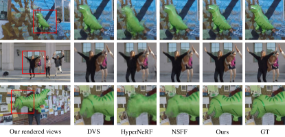
Figure 6: Qualitative comparisons on the Nvidia dataset [75].

Setup.

We estimate camera poses using COLMAP [57]. For each ray, we use a coarse-to-fine sampling strategy with 128 per-ray samples as in Wang et al. [70]. A separate model is trained from scratch for each scene using the Adam optimizer [29]. The network architecture for two main representations is a variant of that of IBRNet [70]. We reconstruct the entire scene in Euclidean space without special scene parameterization. Optimizing a full system on a 10 second video takes around two days using 8 Nvidia A100s, and rendering takes roughly 20 seconds for a $768\times 432$ frame. We refer readers to the supplemental material for network architectures, hyper-parameters setting, and additional details.

5 Evaluation

5.1 Baselines and error metrics

We compare our approach to state-of-the-art monocular view synthesis methods. Specifically, we compare to three recent canonical space–based methods, Nerfies [49], and HyperNeRF [50], and to two scene flow–based methods, NSFF [35] and Dynamic View Synthesis (DVS) from Gao$~{}\emph{et al}.\hbox{}$ [19]. For fair comparisons, we use the same depth, optical flow and motion segmentation masks used for our approach as inputs to other methods.

Following prior work [35], we report the rendering quality of each method with three standard error metrics: peak signal-to-noise ratio (PSNR), structural similarity (SSIM), and perceptual similarity via LPIPS [77], and calculate errors both over the entire scene (Full) and restricted to moving regions (Dynamic Only).

5.2 Quantitative evaluation

Quantitative results on the two benchmark datasets are shown in Table 1 and Table 2. Our approach significantly improves over prior state-of-the-art methods in terms of all error metrics. Notably, our approach improves PSNR over entire scene upon the second best methods by 2dB and 4dB on each of the two datasets. Our approach also reduces LPIPS error, a major indicator of perceptual quality compared with real images [77], by over $50\%$. These results suggest that our framework is much more effective at recovering highly detailed scene contents.

Methods	Full			Dynamic Only
	SSIM$\uparrow$	PSNR$\uparrow$	LPIPS$\downarrow$	SSIM$\uparrow$	PSNR$\uparrow$	LPIPS$\downarrow$
Nerfies [49]	0.823	24.32	0.096	0.595	18.45	0.234
HyperNeRF [50]	0.859	25.10	0.095	0.618	19.26	0.212
DVS [19]	0.943	30.64	0.075	0.866	26.57	0.096
NSFF [35]	0.952	31.75	0.034	0.851	25.83	0.115
Ours	0.983	36.47	0.014	0.909	28.01	0.042

Table 2: Quantitative evaluation on the UCSD dataset [37].

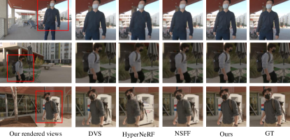
Figure 7: Qualitative comparisons on the UCSD dataset [37].

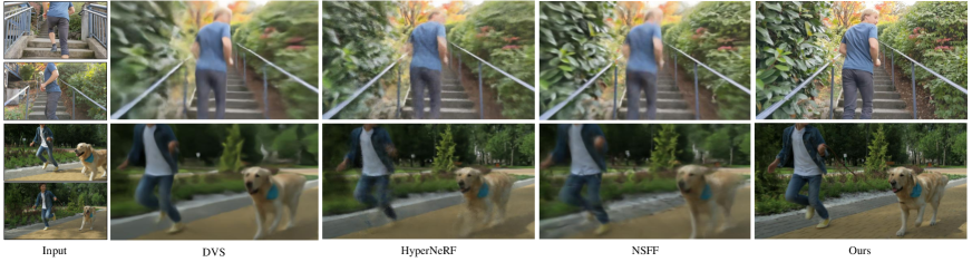
Figure 8: Qualitative comparisons on in-the-wild videos. We show results on 10-second videos of complex dynamic scenes. The leftmost column shows the start and end frames of each video; on the right we show novel views at intermediate times rendered from our approach and prior state-of-the-art methods [19, 50, 35].

Ablation study.

We conduct an ablation study on the Nvidia Dynamic Scene Dataset to validate the effectiveness of our various proposed system components. We show comparisons between our full system and variants in Tab. 3: A) baseline IBRNet [70] with extra time embedding; B) without enforcing temporal consistency via cross-time rendering; C) using scene flow fields to aggregate image features within one time step; D) predicting multiple 3D scene flow vectors pointing to $2r$ nearby times at each sample; E) without using a time-invariant static scene model; F) without masked reconstruction loss via estimated motion segmentation masks; and G) without regularization loss. For this ablation study, we train each model with 64 samples per ray. Without our motion trajectory representation and temporal consistency, view synthesis quality degrades significantly as shown in the first three rows of Tab. 3. Integrating a global spatial coordinate embedding further improves rendering quality. Combining static and dynamic models improves quality for static elements, as seen in metrics over full scenes. Finally, removing supervision from motion segmentation or regularization reduces overall rendering quality, demonstrating the value of proposed losses for avoiding bad local minimal during optimization.

5.3 Qualitative evaluation

Dynamic scenes dataset.

We provide qualitative comparisons between our approach and three prior state-of-the-art methods [19, 35, 50] on the test views from two datasets in Fig. 6 and Fig.7. Prior dynamic-NeRF methods have difficulty rendering details of moving objects, as seen in the excessively blurred dynamic content including the texture of balloons, human faces, and clothing. In contrast, our approach synthesizes photo-realistic novel views of both static and dynamic scene content and which are closest to the ground truth images.

Methods	Full			Dynamic Only
	SSIM$\uparrow$	PSNR$\uparrow$	LPIPS$\downarrow$	SSIM$\uparrow$	PSNR$\uparrow$	LPIPS$\downarrow$
A) [70]+time	0.905	25.33	0.081	0.683	20.09	0.122
B) w/o TC	0.911	27.57	0.074	0.751	22.16	0.104
C) w/ SF	0.935	29.42	0.035	0.797	22.41	0.095
D) w/ M-SF	0.947	29.59	0.033	0.814	22.97	0.084
E) w/o static rep.	0.919	28.19	0.047	0.840	24.01	0.071
F) w/o $\mathcal{L}_{\text{mask}}$	0.930	29.95	0.036	0.835	24.30	0.063
G) w/o $\mathcal{L}_{\text{reg}}$	0.921	29.46	0.042	0.795	22.19	0.080
Full	0.957	30.77	0.028	0.837	24.27	0.066

Table 3: Ablation study on the Nvidia Dataset. See Sec. 5.2 for detailed descriptions of each configuration.

In-the-wild videos.

We show qualitative comparisons on in-the-wild footage of complex dynamic scenes. We show comparisons with Dynamic-NeRF based methods in Fig. 8, and Fig. 9 shows comparisons with point cloud rendering using depths [80] . Our approach synthesizes photo-realistic novel views, whereas prior dynamic-Nerf methods fail to recover high-quality details of both static and moving scene contents, such as the shirt wrinkles and the dog’s fur in Fig. 8. On the other hand, explicit depth warping produces holes at regions near disocculusions and out of field of view. We refer readers to the supplementary video for full comparisons.

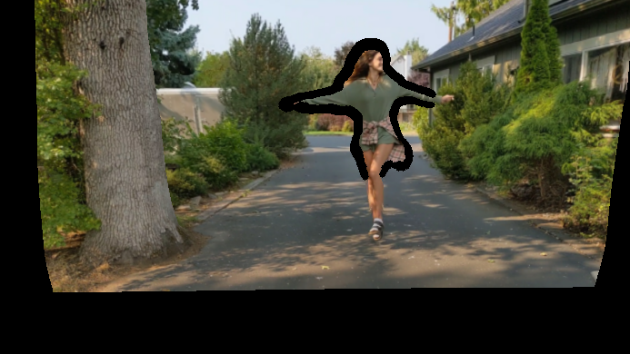
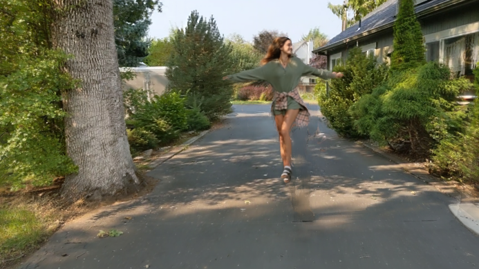
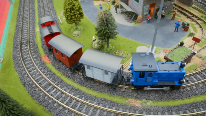
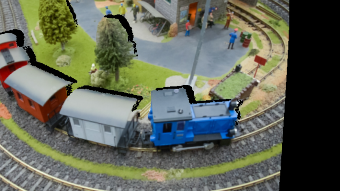
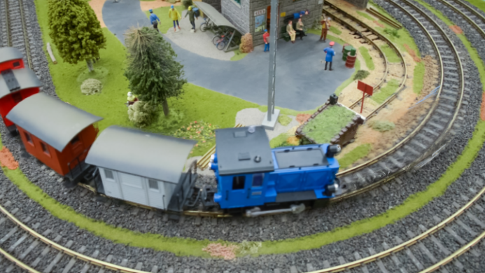
Figure 9: From left to right, We show inputs and corresponding novel views rendered from explicit depth warping with Zhang et al. [80], and from our approach.

6 Discussion and conclusion

Limitations.

Our method is limited to relatively small viewpoint changes compared with methods designed for static or quasi-static scene; Our method is not able to handle small fast moving object due to incorrect initial depth and optical flow estimates (left, Fig. 10). In addition, compared to prior dynamic NeRF methods, the synthesized views are not strictly multi-view consistent, and rendering quality of static content depends on which source views are selected (middle, Fig. 10). Our approach is also sensitive to degenerate motion patterns from in-the-wild videos, in which object and camera motion is mostly colinear, but we show heuristics to handle such cases in the supplemental. Moreover, our method is able to synthesize dynamic contents only appearing at distant time (right, Fig. 10)

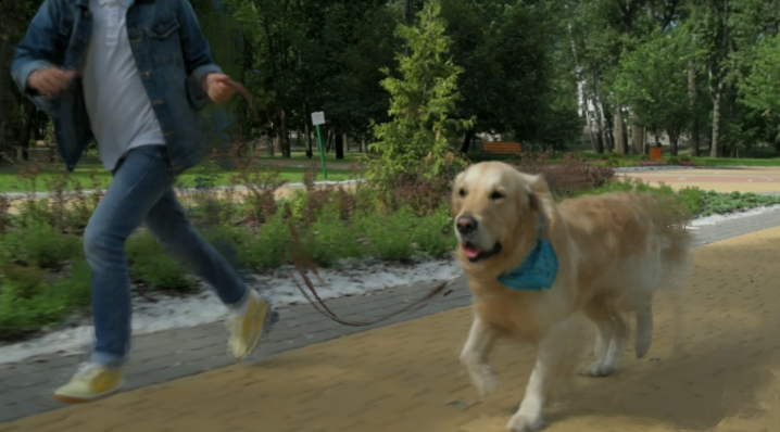
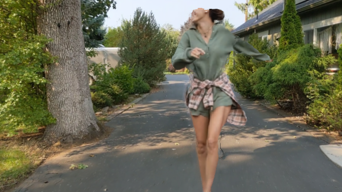
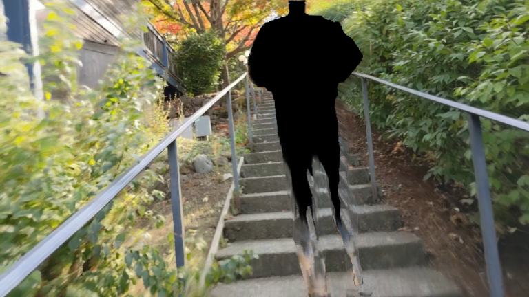
Figure 10: Limitations. Our method might fail to model moving thin objects such as moving leash (left). Our method can fail to render dynamic contents only visible in distant frames (middle). The rendered static content can be unrealistic or blank if insufficient source views feature are aggregated for a given pixel (right).

Conclusion.

We presented a new approach for space-time view synthesis from a monocular video depicting a complex dynamic scene. By representing a dynamic scene within a volumetric IBR framework, our approach overcomes limitations of recent methods that cannot model long videos with complex camera and object motion. We have shown that our method can synthesize photo-realistic novel views from in-the-wild dynamic videos, and can achieve significant improvements over prior state-of-the-art methods on the dynamic scene benchmarks.

Acknowledgements.

Thanks to Andrew Liu, Richard Bowen and Lucy Chai for the fruitful discussions, and thanks to Rick Szeliski and Ricardo Martin-Brualla for helpful proofreading.

References

- [1] Aayush Bansal, Minh Vo, Yaser Sheikh, Deva Ramanan, and Srinivasa Narasimhan. 4D visualization of dynamic events from unconstrained multi-view videos. In Proc. Computer Vision and Pattern Recognition (CVPR), pages 5366–5375, 2020.
- [2] Jonathan T Barron, Ben Mildenhall, Dor Verbin, Pratul P Srinivasan, and Peter Hedman. Mip-NeRF 360: Unbounded anti-aliased neural radiance fields. In Proc. Computer Vision and Pattern Recognition (CVPR), 2022.
- [3] Mojtaba Bemana, Karol Myszkowski, Hans-Peter Seidel, and Tobias Ritschel. X-fields: Implicit neural view-, light-and time-image interpolation. ACM Trans. Graphics, 39(6), 2020.
- [4] Sai Bi, Zexiang Xu, Pratul P. Srinivasan, Ben Mildenhall, Kalyan Sunkavalli, Milovs Havsan, Yannick Hold-Geoffroy, D. Kriegman, and R. Ramamoorthi. Neural reflectance fields for appearance acquisition. ArXiv, abs/2008.03824, 2020.
- [5] Aljaz Bozic, Michael Zollhofer, Christian Theobalt, and Matthias Niessner. Deepdeform: Learning non-rigid RGB-D reconstruction with semi-supervised data. In Proc. Computer Vision and Pattern Recognition (CVPR), June 2020.
- [6] Michael Broxton, John Flynn, Ryan Overbeck, Daniel Erickson, Peter Hedman, Matthew Duvall, Jason Dourgarian, Jay Busch, Matt Whalen, and Paul Debevec. Immersive light field video with a layered mesh representation. ACM Trans. Graph., 39(4), July 2020.
- [7] Chris Buehler, Michael Bosse, Leonard McMillan, Steven Gortler, and Michael Cohen. Unstructured lumigraph rendering. In Proceedings of the 28th annual conference on Computer graphics and interactive techniques, pages 425–432, 2001.
- [8] Joel Carranza, Christian Theobalt, Marcus A Magnor, and Hans-Peter Seidel. Free-viewpoint video of human actors. ACM transactions on graphics (TOG), 22(3):569–577, 2003.
- [9] Jin-Xiang Chai, Xin Tong, Shing-Chow Chan, and Heung-Yeung Shum. Plenoptic sampling. In Proceedings of the 27th Annual Conference on Computer Graphics and Interactive Techniques, SIGGRAPH ’00, page 307–318, USA, 2000. ACM Press/Addison-Wesley Publishing Co.
- [10] Pierre Charbonnier, Laure Blanc-Feraud, Gilles Aubert, and Michel Barlaud. Two deterministic half-quadratic regularization algorithms for computed imaging. In Proceedings of 1st International Conference on Image Processing, volume 2, pages 168–172. IEEE, 1994.
- [11] Anpei Chen, Zexiang Xu, Fuqiang Zhao, Xiaoshuai Zhang, Fanbo Xiang, Jingyi Yu, and Hao Su. MVSNeRF: Fast generalizable radiance field reconstruction from multi-view stereo. In Proceedings of the IEEE/CVF International Conference on Computer Vision, pages 14124–14133, 2021.
- [12] Inchang Choi, Orazio Gallo, Alejandro Troccoli, Min H Kim, and Jan Kautz. Extreme view synthesis. In Proc. Int. Conf. on Computer Vision (ICCV), pages 7781–7790, 2019.
- [13] Edilson De Aguiar, Carsten Stoll, Christian Theobalt, Naveed Ahmed, Hans-Peter Seidel, and Sebastian Thrun. Performance capture from sparse multi-view video. In ACM SIGGRAPH 2008 papers, pages 1–10. 2008.
- [14] Paul E Debevec, Camillo J Taylor, and Jitendra Malik. Modeling and rendering architecture from photographs: A hybrid geometry-and image-based approach. In Proceedings of the 23rd annual conference on Computer graphics and interactive techniques, pages 11–20, 1996.
- [15] Mingsong Dou, Sameh Khamis, Yury Degtyarev, Philip L. Davidson, Sean Ryan Fanello, Adarsh Kowdle, Sergio Orts, Christoph Rhemann, David Kim, Jonathan Taylor, Pushmeet Kohli, Vladimir Tankovich, and Shahram Izadi. Fusion4D: real-time performance capture of challenging scenes. ACM Trans. Graphics, 35:114:1–114:13, 2016.
- [16] Yilun Du, Yinan Zhang, Hong-Xing Yu, Joshua B Tenenbaum, and Jiajun Wu. Neural radiance flow for 4d view synthesis and video processing. In 2021 IEEE/CVF International Conference on Computer Vision (ICCV), pages 14304–14314. IEEE Computer Society, 2021.
- [17] John Flynn, Michael Broxton, Paul Debevec, Matthew DuVall, Graham Fyffe, Ryan Overbeck, Noah Snavely, and Richard Tucker. DeepView: View synthesis with learned gradient descent. In Proc. Computer Vision and Pattern Recognition (CVPR), pages 2367–2376, 2019.
- [18] John Flynn, Ivan Neulander, James Philbin, and Noah Snavely. DeepStereo: Learning to predict new views from the world’s imagery. In Proc. Computer Vision and Pattern Recognition (CVPR), pages 5515–5524, 2016.
- [19] Chen Gao, Ayush Saraf, Johannes Kopf, and Jia-Bin Huang. Dynamic view synthesis from dynamic monocular video. In Proceedings of the IEEE/CVF International Conference on Computer Vision, pages 5712–5721, 2021.
- [20] Hang Gao, Ruilong Li, Shubham Tulsiani, Bryan Russell, and Angjoo Kanazawa. Monocular dynamic view synthesis: A reality check. arXiv preprint arXiv:2210.13445, 2022.
- [21] Steven J Gortler, Radek Grzeszczuk, Richard Szeliski, and Michael F Cohen. The lumigraph. In Proceedings of the 23rd annual conference on Computer graphics and interactive techniques, pages 43–54, 1996.
- [22] Kaiwen Guo, Peter Lincoln, Philip Davidson, Jay Busch, Xueming Yu, Matt Whalen, Geoff Harvey, Sergio Orts-Escolano, Rohit Pandey, Jason Dourgarian, et al. The relightables: Volumetric performance capture of humans with realistic relighting. ACM Transactions on Graphics (ToG), 38(6):1–19, 2019.
- [23] Peter Hedman, Julien Philip, True Price, Jan-Michael Frahm, George Drettakis, and Gabriel Brostow. Deep blending for free-viewpoint image-based rendering. ACM Trans. Graphics, 37(6):1–15, 2018.
- [24] Peter Hedman, Tobias Ritschel, George Drettakis, and Gabriel Brostow. Scalable inside-out image-based rendering. ACM Transactions on Graphics (TOG), 35(6):1–11, 2016.
- [25] Matthias Innmann, Michael Zollhöfer, Matthias Niessner, Christian Theobalt, and Marc Stamminger. VolumeDeform: Real-time volumetric non-rigid reconstruction. In Proc. European Conf. on Computer Vision (ECCV), 2016.
- [26] Nima Khademi Kalantari, Ting-Chun Wang, and Ravi Ramamoorthi. Learning-based view synthesis for light field cameras. ACM Trans. Graphics, 35(6):1–10, 2016.
- [27] Takeo Kanade, Peter Rander, and PJ Narayanan. Virtualized reality: Constructing virtual worlds from real scenes. IEEE multimedia, 4(1):34–47, 1997.
- [28] Yoni Kasten, Dolev Ofri, Oliver Wang, and Tali Dekel. Layered neural atlases for consistent video editing. ACM Transactions on Graphics (TOG), 40(6):1–12, 2021.
- [29] Diederik P. Kingma and Jimmy Ba. Adam: A method for stochastic optimization. CoRR, abs/1412.6980, 2014.
- [30] Johannes Kopf, Michael F Cohen, and Richard Szeliski. First-person hyper-lapse videos. ACM Transactions on Graphics (TOG), 33(4):1–10, 2014.
- [31] Johannes Kopf, Xuejian Rong, and Jia-Bin Huang. Robust consistent video depth estimation. In Proceedings of the IEEE/CVF Conference on Computer Vision and Pattern Recognition, pages 1611–1621, 2021.
- [32] Marc Levoy and Pat Hanrahan. Light field rendering. In Proceedings of the 23rd annual conference on Computer graphics and interactive techniques, pages 31–42, 1996.
- [33] Tianye Li, Mira Slavcheva, Michael Zollhoefer, Simon Green, Christoph Lassner, Changil Kim, Tanner Schmidt, Steven Lovegrove, Michael Goesele, Richard Newcombe, et al. Neural 3D video synthesis from multi-view video. In Proceedings of the IEEE/CVF Conference on Computer Vision and Pattern Recognition, pages 5521–5531, 2022.
- [34] Zhengqi Li, Tali Dekel, Forrester Cole, Richard Tucker, Noah Snavely, Ce Liu, and William T Freeman. Learning the depths of moving people by watching frozen people. In Proc. Computer Vision and Pattern Recognition (CVPR), pages 4521–4530, 2019.
- [35] Zhengqi Li, Simon Niklaus, Noah Snavely, and Oliver Wang. Neural scene flow fields for space-time view synthesis of dynamic scenes. In Proc. Computer Vision and Pattern Recognition (CVPR), 2021.
- [36] Zhengqi Li, Qianqian Wang, Noah Snavely, and Angjoo Kanazawa. Infinitenature-zero: Learning perpetual view generation of natural scenes from single images. In Computer Vision–ECCV 2022: 17th European Conference, Tel Aviv, Israel, October 23–27, 2022, Proceedings, Part I, pages 515–534. Springer, 2022.
- [37] Kai-En Lin, Lei Xiao, Feng Liu, Guowei Yang, and Ravi Ramamoorthi. Deep 3D mask volume for view synthesis of dynamic scenes. In Proc. Int. Conf. on Computer Vision (ICCV), 2021.
- [38] Lingjie Liu, Jiatao Gu, Kyaw Zaw Lin, Tat-Seng Chua, and Christian Theobalt. Neural sparse voxel fields. Advances in Neural Information Processing Systems, 33:15651–15663, 2020.
- [39] Yuan Liu, Sida Peng, Lingjie Liu, Qianqian Wang, Peng Wang, Christian Theobalt, Xiaowei Zhou, and Wenping Wang. Neural rays for occlusion-aware image-based rendering. In CVPR, 2022.
- [40] Stephen Lombardi, Tomas Simon, Jason Saragih, Gabriel Schwartz, Andreas Lehrmann, and Yaser Sheikh. Neural volumes: Learning dynamic renderable volumes from images. ACM Trans. Graphics, 38(4):65, 2019.
- [41] Matthew Loper, Naureen Mahmood, Javier Romero, Gerard Pons-Moll, and Michael J Black. SMPL: A skinned multi-person linear model. ACM transactions on graphics (TOG), 34(6):1–16, 2015.
- [42] Erika Lu, F. Cole, Tali Dekel, Weidi Xie, Andrew Zisserman, D. Salesin, W. Freeman, and M. Rubinstein. Layered neural rendering for retiming people in video. ACM Trans. Graphics (SIGGRAPH Asia), 2020.
- [43] Erika Lu, Forrester Cole, Tali Dekel, Andrew Zisserman, William T Freeman, and Michael Rubinstein. Omnimatte: Associating objects and their effects in video. In Proc. Computer Vision and Pattern Recognition (CVPR), 2021.
- [44] Xuan Luo, Jia-Bin Huang, Richard Szeliski, Kevin Matzen, and Johannes Kopf. Consistent video depth estimation. ACM Trans. Graph., 39(4), July 2020.
- [45] Ricardo Martin-Brualla, N. Radwan, Mehdi S. M. Sajjadi, J. Barron, A. Dosovitskiy, and Daniel Duckworth. NeRF in the wild: Neural radiance fields for unconstrained photo collections. In Proc. Computer Vision and Pattern Recognition (CVPR), 2021.
- [46] Ben Mildenhall, Pratul P Srinivasan, Matthew Tancik, Jonathan T Barron, Ravi Ramamoorthi, and Ren Ng. NeRF: Representing scenes as neural radiance fields for view synthesis. Proc. European Conf. on Computer Vision (ECCV), 2020.
- [47] Richard A Newcombe, Dieter Fox, and Steven M Seitz. DynamicFusion: Reconstruction and tracking of non-rigid scenes in real-time. In Proc. Computer Vision and Pattern Recognition (CVPR), 2015.
- [48] Michael Niemeyer, Lars Mescheder, Michael Oechsle, and Andreas Geiger. Differentiable volumetric rendering: Learning implicit 3D representations without 3D supervision. In Proceedings of the IEEE/CVF Conference on Computer Vision and Pattern Recognition, pages 3504–3515, 2020.
- [49] Keunhong Park, Utkarsh Sinha, Jonathan T Barron, Sofien Bouaziz, Dan B Goldman, Steven M Seitz, and Ricardo Martin-Brualla. Nerfies: Deformable neural radiance fields. In Proceedings of the IEEE/CVF International Conference on Computer Vision, pages 5865–5874, 2021.
- [50] Keunhong Park, Utkarsh Sinha, Peter Hedman, Jonathan T Barron, Sofien Bouaziz, Dan B Goldman, Ricardo Martin-Brualla, and Steven M Seitz. HyperNeRF: A higher-dimensional representation for topologically varying neural radiance fields. arXiv preprint arXiv:2106.13228, 2021.
- [51] Sida Peng, Yuanqing Zhang, Yinghao Xu, Qianqian Wang, Qing Shuai, Hujun Bao, and Xiaowei Zhou. Neural body: Implicit neural representations with structured latent codes for novel view synthesis of dynamic humans. In Proceedings of the IEEE/CVF Conference on Computer Vision and Pattern Recognition, pages 9054–9063, 2021.
- [52] Eric Penner and Li Zhang. Soft 3D reconstruction for view synthesis. ACM Trans. Graphics, 36(6):1–11, 2017.
- [53] Albert Pumarola, Enric Corona, Gerard Pons-Moll, and Francesc Moreno-Noguer. D-NeRF: Neural radiance fields for dynamic scenes. In Proceedings of the IEEE/CVF Conference on Computer Vision and Pattern Recognition, pages 10318–10327, 2021.
- [54] Gernot Riegler and V. Koltun. Free view synthesis. Proc. European Conf. on Computer Vision (ECCV), 2020.
- [55] Gernot Riegler and Vladlen Koltun. Stable view synthesis. In Proceedings of the IEEE/CVF Conference on Computer Vision and Pattern Recognition, pages 12216–12225, 2021.
- [56] Shunsuke Saito, Zeng Huang, Ryota Natsume, Shigeo Morishima, Angjoo Kanazawa, and Hao Li. PIFu: Pixel-aligned implicit function for high-resolution clothed human digitization. In Proceedings of the IEEE/CVF International Conference on Computer Vision, pages 2304–2314, 2019.
- [57] Johannes L Schonberger and Jan-Michael Frahm. Structure-from-motion revisited. In Proc. Computer Vision and Pattern Recognition (CVPR), pages 4104–4113, 2016.
- [58] Harry Shum and Sing Bing Kang. Review of image-based rendering techniques. In Visual Communications and Image Processing 2000, volume 4067, pages 2–13. SPIE, 2000.
- [59] Vincent Sitzmann, Julien Martel, Alexander Bergman, David Lindell, and Gordon Wetzstein. Implicit neural representations with periodic activation functions. Advances in Neural Information Processing Systems, 33:7462–7473, 2020.
- [60] Vincent Sitzmann, Justus Thies, Felix Heide, Matthias Nießner, Gordon Wetzstein, and Michael Zollhofer. Deepvoxels: Learning persistent 3D feature embeddings. In Proc. Computer Vision and Pattern Recognition (CVPR), pages 2437–2446, 2019.
- [61] Vincent Sitzmann, Michael Zollhöfer, and Gordon Wetzstein. Scene representation networks: Continuous 3D-structure-aware neural scene representations. In Neural Information Processing Systems, pages 1119–1130, 2019.
- [62] Pratul P Srinivasan, Richard Tucker, Jonathan T Barron, Ravi Ramamoorthi, Ren Ng, and Noah Snavely. Pushing the boundaries of view extrapolation with multiplane images. In Proc. Computer Vision and Pattern Recognition (CVPR), pages 175–184, 2019.
- [63] Timo Stich, Christian Linz, Georgia Albuquerque, and Marcus Magnor. View and time interpolation in image space. In Computer Graphics Forum, volume 27, pages 1781–1787. Wiley Online Library, 2008.
- [64] Mohammed Suhail, Carlos Esteves, Leonid Sigal, and Ameesh Makadia. Light field neural rendering. In Proc. Computer Vision and Pattern Recognition (CVPR), 2022.
- [65] Zachary Teed and Jia Deng. RAFT: Recurrent all-pairs field transforms for optical flow. In Proc. European Conf. on Computer Vision (ECCV), 2020.
- [66] Edgar Tretschk, Ayush Tewari, Vladislav Golyanik, Michael Zollhöfer, Christoph Lassner, and Christian Theobalt. Non-rigid neural radiance fields: Reconstruction and novel view synthesis of a dynamic scene from monocular video. In Proceedings of the IEEE/CVF International Conference on Computer Vision, pages 12959–12970, 2021.
- [67] Chaoyang Wang, Ben Eckart, Simon Lucey, and Orazio Gallo. Neural trajectory fields for dynamic novel view synthesis. arXiv preprint arXiv:2105.05994, 2021.
- [68] Chaoyang Wang, Xueqian Li, Jhony Kaesemodel Pontes, and Simon Lucey. Neural prior for trajectory estimation. In Proceedings of the IEEE/CVF Conference on Computer Vision and Pattern Recognition, pages 6532–6542, 2022.
- [69] Liao Wang, Jiakai Zhang, Xinhang Liu, Fuqiang Zhao, Yanshun Zhang, Yingliang Zhang, Minye Wu, Jingyi Yu, and Lan Xu. Fourier plenoctrees for dynamic radiance field rendering in real-time. In Proceedings of the IEEE/CVF Conference on Computer Vision and Pattern Recognition, pages 13524–13534, 2022.
- [70] Qianqian Wang, Zhicheng Wang, Kyle Genova, Pratul P Srinivasan, Howard Zhou, Jonathan T Barron, Ricardo Martin-Brualla, Noah Snavely, and Thomas Funkhouser. Ibrnet: Learning multi-view image-based rendering. In Proc. Computer Vision and Pattern Recognition (CVPR), pages 4690–4699, 2021.
- [71] Chung-Yi Weng, Brian Curless, Pratul P Srinivasan, Jonathan T Barron, and Ira Kemelmacher-Shlizerman. HumanNeRF: Free-viewpoint rendering of moving people from monocular video. In Proceedings of the IEEE/CVF Conference on Computer Vision and Pattern Recognition, pages 16210–16220, 2022.
- [72] Suttisak Wizadwongsa, Pakkapon Phongthawee, Jiraphon Yenphraphai, and Supasorn Suwajanakorn. NeX: Real-time view synthesis with neural basis expansion. In Proceedings of the IEEE/CVF Conference on Computer Vision and Pattern Recognition, pages 8534–8543, 2021.
- [73] Tianhao Wu, Fangcheng Zhong, Andrea Tagliasacchi, Forrester Cole, and Cengiz Oztireli. D2NeRF: Self-supervised decoupling of dynamic and static objects from a monocular video. arXiv preprint arXiv:2205.15838, 2022.
- [74] Wenqi Xian, Jia-Bin Huang, Johannes Kopf, and Changil Kim. Space-time neural irradiance fields for free-viewpoint video. In Proceedings of the IEEE/CVF Conference on Computer Vision and Pattern Recognition, pages 9421–9431, 2021.
- [75] Jae Shin Yoon, Kihwan Kim, Orazio Gallo, Hyun Soo Park, and Jan Kautz. Novel view synthesis of dynamic scenes with globally coherent depths from a monocular camera. In Proc. Computer Vision and Pattern Recognition (CVPR), pages 5336–5345, 2020.
- [76] Jiakai Zhang, Xinhang Liu, Xinyi Ye, Fuqiang Zhao, Yanshun Zhang, Minye Wu, Yingliang Zhang, Lan Xu, and Jingyi Yu. Editable free-viewpoint video using a layered neural representation. ACM Transactions on Graphics (TOG), 40(4):1–18, 2021.
- [77] Richard Zhang, Phillip Isola, Alexei A Efros, Eli Shechtman, and Oliver Wang. The unreasonable effectiveness of deep features as a perceptual metric. In Proc. Computer Vision and Pattern Recognition (CVPR), pages 586–595, 2018.
- [78] Zhoutong Zhang, Forrester Cole, Zhengqi Li, Michael Rubinstein, Noah Snavely, and William T Freeman. Structure and motion from casual videos. In European Conference on Computer Vision, pages 20–37. Springer, 2022.
- [79] Zhoutong Zhang, Forrester Cole, Zhengqi Li, Noah Snavely, and William Freeman. Structure and motion from casual videos. In Proc. European Conf. on Computer Vision (ECCV), 2022.
- [80] Zhoutong Zhang, Forrester Cole, Richard Tucker, William T Freeman, and Tali Dekel. Consistent depth of moving objects in video. ACM Transactions on Graphics (TOG), 40(4):1–12, 2021.
- [81] Tinghui Zhou, Richard Tucker, John Flynn, Graham Fyffe, and Noah Snavely. Stereo magnification: learning view synthesis using multiplane images. ACM Trans. Graphics, 37:1 – 12, 2018.
- [82] C Lawrence Zitnick, Sing Bing Kang, Matthew Uyttendaele, Simon Winder, and Richard Szeliski. High-quality video view interpolation using a layered representation. ACM Trans. Graphics, 23(3):600–608, 2004.
- [83] Michael Zollhöfer, Matthias Niessner, Shahram Izadi, Christoph Rehmann, Christopher Zach, Matthew Fisher, Chenglei Wu, Andrew Fitzgibbon, Charles Loop, Christian Theobalt, et al. Real-time non-rigid reconstruction using an RGB-D camera. ACM Trans. Graphics, 33(4):156, 2014.