When Noisy Labels Meet Long Tail Dilemmas:
A Representation Calibration Method

Abstract

Real-world large-scale datasets are both noisily labeled and class-imbalanced. The issues seriously hurt the generalization of trained models. It is hence significant to address the simultaneous incorrect labeling and class-imbalance, i.e., the problem of learning with noisy labels on long-tailed data. Previous works develop several methods for the problem. However, they always rely on strong assumptions that are invalid or hard to be checked in practice. In this paper, to handle the problem and address the limitations of prior works, we propose a representation calibration method RCAL. Specifically, RCAL works with the representations extracted by unsupervised contrastive learning. We assume that without incorrect labeling and class imbalance, the representations of instances in each class conform to a multivariate Gaussian distribution, which is much milder and easier to be checked. Based on the assumption, we recover underlying representation distributions from polluted ones resulting from mislabeled and class-imbalanced data. Additional data points are then sampled from the recovered distributions to help generalization. Moreover, during classifier training, representation learning takes advantage of representation robustness brought by contrastive learning, which further improves the classifier performance. We derive theoretical results to discuss the effectiveness of our representation calibration. Experiments on multiple benchmarks justify our claims and confirm the superiority of the proposed method.

1 Introduction

Deep learning has made rapid progress in many fields [16], primarily driven by large-scale and high-quality annotated datasets [30, 5, 18, 71, 62, 35]. Unfortunately, it is hard to obtain such perfect datasets in practice, mainly from two aspects: (1) a part of data is wrongly labeled due to its intrinsic ambiguity and mistakes of annotators [44, 34, 66, 60, 37]; (2) data is class-imbalanced, where a long-tailed class distribution exhibits [55, 83, 24]. In real-world settings, both imperfect situations usually coexist (see Figure 1). For example, the WebVision dataset [36], a large-scale image dataset crawled from the web, contains about $20\%$ mislabeled data. Meanwhile, the number of examples in the most frequent class is over 20 times that of examples in the most scarce class [28].

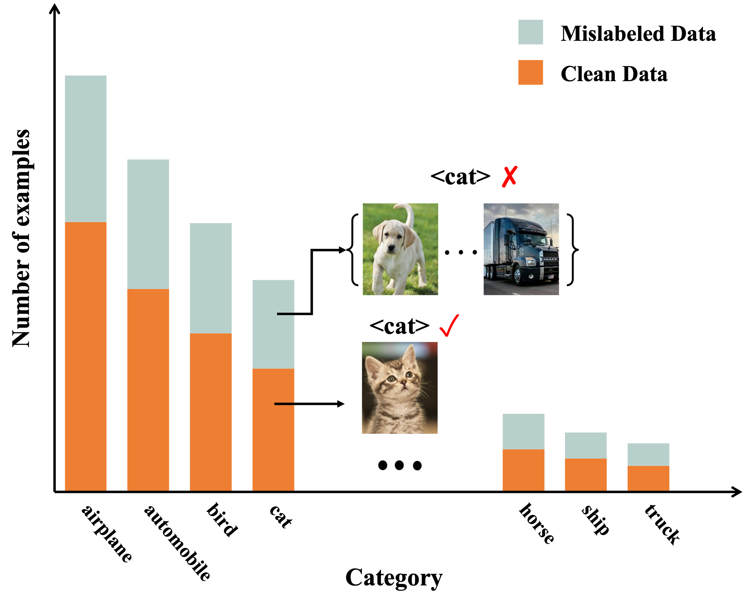
Figure 1: The illustration of the problem setup. The observed data exhibit a long-tailed distribution. The number of clean data and mislabeled data varies in each class.

Although many previous works have emerged to address the problems of learning with noisy labels and learning with long-tailed data separately, they cannot work well when the two imperfect situations exist simultaneously. Namely, they are weak for learning with noisy labels on long-tailed data. Concretely, the methods specialized for learning with noisy labels always rely on some assumptions. Nevertheless, the assumptions are invalid due to the long-tailed issue. For example, the popularly used memorization effect [18] for tackling noisy labels cannot be applied, since clean data belonging to tail classes show similar training dynamics to those mislabeled data, e.g., similar training losses [5, 64]. Also, the noise transition matrix used for handling noisy labels cannot be estimated accurately. This results from that the relied anchor points of tail classes cannot be identified from noisy data, as the estimations of noisy class posterior probabilities for tail classes are not accurate. Moreover, the methods specialized for learning with long-tailed data mainly adopt re-sampling and re-weighting techniques to balance the classifier. The side-effect of mislabeled data is not taken into consideration, which results in the accumulation of label errors.

The weaknesses of the above specialized methods motivate us to develop more advanced methods for the realistic problem of learning with noisy labels on long-tailed data. Existing methods targeting this problem can be divided into two main categories. The methods in the first category are to distinguish mislabeled data from the data of tail classes for follow-up procedures. However, the distinguishment is adversely affected by mislabeled data, since the information used for the distinguishment comes from deep networks that are trained on noisy long-tailed data. The methods in the second category are to reduce the side-effects of mislabeled data and long-tailed data in a unified way, relying on strong assumptions. For example, partial data should have the same aleatoric uncertainty [5], which is hard to check in practice.

In this paper, we focus on this realistic problem: learning with noisy labels on long-tailed data. To address the issues of prior works, we propose a representation calibration method named RCAL. Generally, RCAL works on the level of deep representations, i.e., extracted features by deep networks for instances. Technically, we first employ unsupervised contrastive learning to achieve representations for all training instances. As the procedure of representation learning is not influenced by corrupted training labels, the achieved representations are naturally robust [81, 69, 15]. Afterward, based upon the achieved representations, two representation calibration strategies are performed: distributional and individual representation calibrations.

In more detail, the distributional representation calibration aims to recover representation distributions before data corruption. Specifically, we assume that before training data are corrupted, the deep representations of instances in each class conform to a multivariate Gaussian distribution. Compared to the previously mentioned assumptions, the assumption used in this paper is much milder. Its rationality is also justified by many works [70, 55, 75]. With a density-based outlier detector, robust estimations of multivariate Gaussian distributions are obtained. Moreover, since the insufficient data of tail classes may cause biased distribution estimations, the statistics of distributions from head classes are employed to calibrate the estimations for tail classes. After the distributional calibration for all classes, we sample multiple data points from the recovered distributions, which makes training data more balanced and helps generalization. As for individual representation calibration, considering that the representations obtained by contrastive learning are robust, we restrict that the subsequent learned representations during training are close to them. The individual representation calibration implicitly reduces the hypothesis space of deep networks, which mitigates their overfitting of mislabeled and long-tailed data. Through the above procedure of representation calibration, the learned representations on noisy long-tailed data are calibrated towards uncontaminated representations. The robustness of deep networks is thereby enhanced with such calibrated representations, following better classification performance.

The contributions of this paper are listed as follows: (1) We focus on learning with noisy labels on long-tailed data, which is a realistic but challenging problem. The weaknesses of previous works are carefully discussed. (2) We propose an advanced method RCAL for learning with noisy labels on long-tailed data. Our method benefits from the representations by contrastive learning, where two types of representation calibration strategies are proposed to improve network robustness. (3) We derive theoretical results to confirm the effectiveness of our calibration strategies under some conditions. (4) We conduct extensive experiments on both simulated and real-world datasets. The results demonstrate our representation calibration method’s superiority over existing state-of-the-art methods. In addition, detailed ablation studies and discussions are provided.

2 Related Works

Learning with noisy labels.  There is a series of works proposed to deal with noisy labels, which includes but is not limited to estimating the noise transition matrix [65, 10, 72], selecting confident examples [49, 59, 47], reweighting examples [50, 43], and correcting wrong labels [41]. Additionally, some state-of-the-art methods combine multiple techniques, e.g., DivideMix [32], ELR+ [42], and Sel-CL+ [34].

Learning with long-tailed data.  Existing methods tackling long-tailed data mainly focus on: (1) re-balancing data distributions, such as over-sampling [17, 4, 49], under-sampling [13, 4, 19], and class-balanced sampling [46, 51]; (2) re-designing loss functions, which includes class-level re-weighting [11, 6, 23, 31, 57, 56] and instance-level re-weighting [38, 52, 50, 80]; (3) decoupling representation learning and classifier learning [27, 76]; (4) transfer learning from head knowledge to tail classes [24, 39, 22].

Learning with noisy labels on long-tailed data.  A line of research has made progress towards simultaneously learning with imbalanced data and noisy labels. CurveNet [26] exploits the informative loss curve to identify different biased data types and produces proper example weights in a meta-learning manner, where a small additional unbiased data set is required. HAR [5] proposes a heteroskedastic adaptive regularization approach to handle the joint problem in a unified way. The examples with high uncertainty and low density will be assigned larger regularization strengths. RoLT [61] claims the failure of the small-loss trick in long-tailed learning and designs a prototypical error detection method to better differentiate the mislabeled examples from rare examples. TBSS [77] designs two metrics to detect mislabeled examples under long-tailed data distribution. A semi-supervised technique is then applied.

3 Methodology

3.1 Preliminaries

Notation.  In the sequel, scalars are in lowercase letters. Vectors are in lowercase boldface letters. Let $[z]=\{1,2,\ldots,z\}$. Besides, $|\mathcal{B}|$ denotes the total number of elements in the set $\mathcal{B}$.

Problem setup.  We consider a $K$-class classification problem, where $K\geq 2$. We are given an imbalanced and noisily labeled training dataset $\tilde{\mathcal{S}}=\{(\bm{x}_{i},\tilde{y}_{i})\}_{i=1}^{n}$, where $n$ is the sample size, $\bm{x}_{i}$ denotes the $i$-th instance and its label $\tilde{y}_{i}\in[K]$ may be incorrect. For the label $\tilde{y}_{i}$, the corresponding true label is denoted by $y_{i}$, which is unobservable. Let the number of training data belonging to $k$-th class be $n_{k}$. Without loss of generality, we suppose that the classes are sorted in decreasing order, based on the number of training data in each class, i.e., $n_{1}\geq...\geq n_{K}$. Afterward, all classes can be recognized into two parts: head classes (referred as $\mathcal{G}_{h}$) and tail classes (referred as $\mathcal{G}_{t}$). In this paper, the aim is to learn a classifier robustly by only using the imbalanced and noisily labeled training dataset, which can infer proper labels for unseen instances.

Algorithm overview.  In the following, we discuss the proposed method RCAL step by step. Generally, RCAL consists of two stages: (1) the stage of representation enhancements by contrastive learning; (2) the stage of improving the classifier’s robustness by representation calibration, which is performed with before enhanced representations. The procedure of RCAL is illustrated in Figure 2. We provide more technical details of our method as follows.

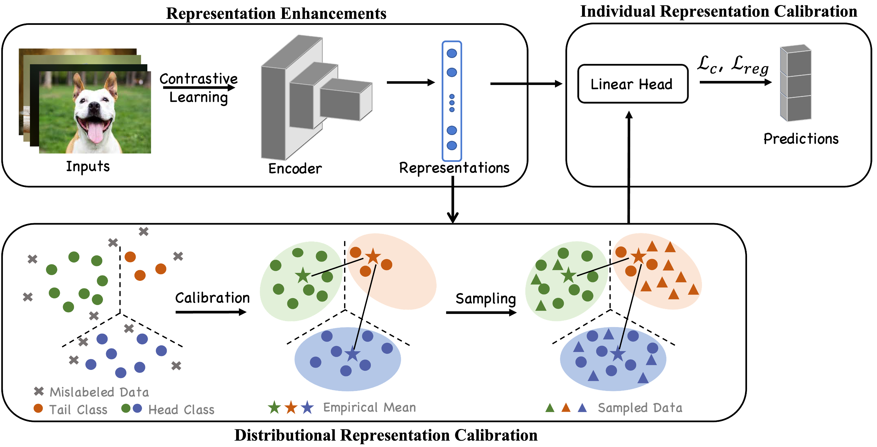
Figure 2: The illustration of the proposed method, uses the representations achieved by contrastive learning for follow-up distributional and individual representation calibrations.

3.2 Enhancing Representations Through Contrastive Learning

To improve the robustness of deep representations of instances for handling noisy labels in long-tailed cases, we exploit self-supervised contrastive learning. Intuitively, as the representation learning in self-supervised contrastive learning does not access the labels of training data, the achieved representations will not be influenced by incorrect labels [69]. Besides, prior work [40] shows that contrastive learning can improve the network tolerance to long-tailed data. Therefore, deep representations achieved with contrastive learning help tackle noisy labels in long-tailed cases.

Specifically, we utilize the encoder networks following the popular setup in MOCO [9]. For an input $\bm{x}$, we apply two random augmentations and thus generate two views $\bm{x}^{q}$ and $\bm{x}^{k}$. The two views are then fed into a query encoder $f(\cdot)$ and a key encoder $f^{\prime}(\cdot)$, which generates representations $\bm{z}^{q}=f(\bm{x}^{q})$ and $\bm{z}^{k}=f^{\prime}(\bm{x}^{k})$. Thereafter, a projection head, i.e., a 2-layer MLP, maps the two representations to lower-dimensional embeddings $\hat{\bm{z}}^{q}$ and $\hat{\bm{z}}^{k}$. MOCO also maintains a large queue to learn good representations. The key encoder uses a momentum update with the query encoder to keep the queue as consistent as possible. The contrastive loss for the input $\bm{x}_{i}$ can be expressed as:

$$\mathcal{L}_{con}(\bm{x}_{i})=-\log\frac{\exp(\hat{\bm{z}}_{i}^{q}\cdot\hat{\bm{z}}_{i}^{k}/\tau)}{\Sigma_{\hat{\bm{z}}^{k^{\prime}}\in\mathcal{A}}\exp(\hat{\bm{z}}_{i}^{q}\cdot\hat{\bm{z}}^{k^{\prime}}/\tau)},$$ (1)

where $\mathcal{A}$ is the queue, and $\tau>0$ is a temperature parameter. The enhanced representation of the input $\bm{x}_{i}$ is achieved by minimizing the loss in Eq. (1). The representation $\bm{z}^{q}=f(\bm{x})$ (simplified as $\bm{z}$) is extracted from the query encoder for later representation distribution calibration.

3.3 Distributional Representation Calibration

In this paper, we assume that before corruption by class-imbalanced noisy labels, the deep representations of training data in each class conform to a multivariate Gaussian distribution. Note that the assumption is applied to deep representations but not original instances, since deep representations are more informative for following procedures. Besides, the assumption is mild and has been verified by existing works [70, 67, 75, 55].

For $K$ classes, we have $K$ multivariate Gaussian distributions. The distribution belonging to the $k$-th class is denoted by $\mathcal{N}(f(\bm{x})|\bm{\mu}_{k},\bm{\Sigma}_{k})$ with $\bm{\mu}_{k}\in\mathbbm{R}^{m}$ and $\bm{\Sigma}_{k}\in\mathbbm{R}^{m\times m}$, where $m$ denotes the dimension of the deep representation. Although without introducing class labels in representation learning by contrastive learning, there is a clustering effect for the obtained representations [81]. Therefore, we can exploit them for modeling the multivariate Gaussian distributions at a class level. Due to the side-effect of mislabeled data, the prior multivariate Gaussian distributions are corrupted. As mentioned, we tend to tackle noisy labels in long-tailed cases, with representation distribution calibration. Therefore, we need to estimate the multivariate Gaussian distributions that are not affected by mislabeled data.

Robust estimations of Gaussian distributions.  If deep representations are not contaminated due to mislabeled data, the empirical mean has a $L_{2}$-error at most $\mathcal{O}(\sqrt{m/n_{k}})$ from the true mean $\bm{\mu}_{k}$. Owing to the existence of noisy labels, the empirical estimation fails. We therefore develop an advanced estimation method. Note that the representations learned from contrastive learning are clustered among similar representations and not influenced by noisy labels. They hence can help detect outliers in the representation space for the estimations of Gaussian distributions.

Technically, given the learned representations $\bm{z}$, we employ the Local Outlier Factor (LOF) algorithm [3] to detect outliers. The outliers are then removed for the following estimation. After performing the LOF algorithm on $\{(\bm{z}_{i},\tilde{y}_{i})\}_{i=1}^{n}$, we segregate clean data for each class. The set of preserved examples for the $k$-th class is denoted by $\tilde{\mathcal{S}}^{\prime}_{k}$, where $\tilde{\mathcal{S}}^{\prime}_{k}=\{(\bm{z}_{i},\tilde{y}_{i})\}_{i=1}^{|\tilde{\mathcal{S}}^{\prime}_{k}|}$ with $|\tilde{\mathcal{S}}^{\prime}_{k}|<n_{k}$. With $\tilde{\mathcal{S}}^{\prime}_{k}$, we estimate the multivariate Gaussian distribution as

$$\hat{\bm{\mu}}_{k}=\sum_{\{i|(\bm{z}_{i},\tilde{y}_{i})\in\tilde{\mathcal{S}}^{\prime}_{k}\}}\frac{\bm{z}_{i}}{|\tilde{\mathcal{S}}^{\prime}_{k}|},$$

$$\hat{\bm{\Sigma}}_{k}=\sum_{\{i|(\bm{z}_{i},\tilde{y}_{i})\in\tilde{\mathcal{S}}^{\prime}_{k}\}}\frac{(\bm{z}_{i}-\hat{\bm{\mu}}_{k})(\bm{z}_{i}-\hat{\bm{\mu}}_{k})^{\top}}{|\tilde{\mathcal{S}}^{\prime}_{k}|-1},$$

where the mean of representation vectors is calculated as the mean of every single dimension in the vector.

Further calibration for tail classes.  As the size of the training data belonging to tail classes is small, it may not be enough for accurately estimating their multivariate Gaussian distributions with the above robust estimation. Inspired by similar classes having similar means and covariance on representations [70, 55], we further borrow the statistics of head classes to assist the calibration of tail classes. Specifically, we measure the similarity by computing the Euclidean distances between the means of representations of different classes. For the tail class $k$, we select top $q$ head classes with the closest Euclidean distance to the mean $\hat{\bm{\mu}}_{k}$:

$$\mathcal{B}_{k} =\left\{-||\hat{\bm{\mu}}_{i}-\hat{\bm{\mu}}_{k}||^{2}\ \big{|}\ i\in\mathcal{G}_{h}\right\},$$

$$\mathcal{C}^{q}_{k} =\left\{i\ \big{|}-||\hat{\bm{\mu}}_{i}-\hat{\bm{\mu}}_{k}||^{2}\in\texttt{topq}(\mathcal{B}_{k})\right\}.$$

Afterward, we can rectify the means and covariances of tail classes as follows:

$$\omega_{c}^{k} =\frac{n_{c}||\hat{\bm{\mu}}_{c}-\hat{\bm{\mu}}_{k}||^{2}}{\sum_{j\in\mathcal{C}^{q}_{k}}n_{j}||\hat{\bm{\mu}}_{j}-\hat{\bm{\mu}}_{k}||^{2}},$$

$$\hat{\bm{\mu}}_{k}^{\prime} =\gamma\sum_{c\in\mathcal{C}^{q}_{k}}\omega_{c}^{k}\hat{\bm{\mu}}_{c}+(1-\gamma)\hat{\bm{\mu}}_{k},$$

$$\hat{\bm{\Sigma}}_{k}^{\prime} =\gamma\sum_{c\in\mathcal{C}^{q}_{k}}\omega_{c}^{k}\hat{\bm{\Sigma}}_{c}+(1-\gamma)\hat{\bm{\Sigma}}_{k}+\alpha\mathbf{1},$$

where $\omega_{c}^{k}$ is the weight that is about using the statistics of the head class $c$ to help the calibration of the tail class $k$. The head classes that are more similar to the tail class $k$ will be endowed with smaller weights. Additionally, $\gamma$ is the confidence on the statistics computed from head classes, $\mathbf{1}\in\mathbbm{R}^{m\times m}$ is the matrix of ones, and $\alpha\in\mathbbm{R}^{+}$ is a hyperparameter that controls the degree of disturbance. The application of the disturbance can make the estimations of covariances more robust. At last, the multivariate Gaussian distributions for head classes are achieved by $\mathcal{N}(\bm{z}|\hat{\bm{\mu}},\hat{\bm{\Sigma}})$, while the multivariate Gaussian distributions for tail classes are calibrated and given by $\mathcal{N}(\bm{z}|\hat{\bm{\mu}}^{\prime},\hat{\bm{\Sigma}}^{\prime})$.

After recovering all multivariate Gaussian distributions, we sample multiple data points from them for classifier training. As the recovered distributions are close to the representation distributions of clean data, training with these sampled data points can make the classifier more robust. Furthermore, we can control the number of sampled data points from different classes to make training data more balanced, which helps generalization.

3.4 Individual Representation Calibration

Before this, we finish distributional representation calibration to recover the multivariate Gaussian distributions. Going a further step to improve the representation robustness, we perform individual representation calibration which includes two parts.

First, considering that self-supervised contrastive learning provides us robust representations (Section 3.2), we restrict the distance between subsequent learned representations and the representations brought by contrastive learning. Specifically, we denote the representations brought by contrastive learning as $\bm{z}^{0}$. Then the distance restriction is formulated as

$$\mathcal{L}_{reg}(\bm{x})=||\bm{z}-\bm{z}^{0}||^{2}=||f(\bm{x})-\bm{z}^{0}||^{2}.$$

Second, to further make learned representations robust to tackle noisy labels in long-tailed cases, we employ the mixup method [74]. Let the cross-entropy loss for the example $(\bm{x},\tilde{y})$ be $\mathcal{L}_{c}(\bm{x},\tilde{y})$. In the procedure of mixup, each time we randomly sample two examples $(\bm{x}_{i},\tilde{y}_{i})$ and $(\bm{x}_{j},\tilde{y}_{j})$, weighted combinations of these two examples are generated as

$$\bm{x}_{i,j}=\lambda\bm{x}_{i}+(1-\lambda)\bm{x}_{j}\ \text{and}\ \tilde{y}_{i,j}=\lambda\tilde{y}_{i}+(1-\lambda)\tilde{y}_{j},$$

where $\lambda\in[0,1]$ is drawn from the Beta distribution. Accordingly, the original training objective based on the cross-entropy loss is replaced with $\mathcal{L}_{c}(\bm{x}_{i,j},\tilde{y}_{i,j})$. Note that, for the classification, we add a linear head $h$. The classification results of the instance $\bm{x}$ are $h(f(\bm{x}))$. Finally, the overall objective is formulated as

$$\mathcal{L}=\mathcal{L}_{c}+\beta\mathcal{L}_{reg},$$ (2)

where $\beta$ controls the strength of distance regularization. The algorithm flow of our method is provided in Algorithm 1.

Algorithm 1 Algorithm of the proposed method RCAL

0:  the training dataset $\tilde{\mathcal{S}}=\{(\bm{x}_{i},\tilde{y}_{i}\})_{i=1}^{n}$, regularization strength $\beta$, scalar temperature $\tau$, confidence weight $\gamma$, the pre-training epochs $T_{p}$, max epochs $T_{m}$.

1:  for $t=1,...,T_{p}$ do

2:     Pre-train the encoder network $f$ with MoCo [20].

3:  end for

4:  Extract deep representations of instances with $\bm{z}=f(\bm{x})$.

5:  for $c=1,...,K$ do

6:     Perform the LOF algorithm for the $c$-th class and obtain preserved examples $\tilde{\mathcal{S}}^{\prime}_{c}$.

7:     Build the multivariate Gaussian distribution $\mathcal{N}(f(\bm{x})|\hat{\bm{\mu}}_{c},\hat{\bm{\Sigma}}_{c})$ for $c$-th class using $\tilde{\mathcal{S}}^{\prime}_{c}$.

8:  end for

9:  Calibrate the multivariate Gaussian distributions of tail classes with the statistics of head classes.

10:  Sample data points from achieved multivariate Gaussian distributions of all classes.

11:  for $t=T_{p}+1,...,T_{m}$ do

12:     Add distance constraints between learned representations and representations brought by contrastive learning.

13:     Adopt the mixup technology to original examples.

14:     Train the encoder $f$ and the linear head $h$ simultaneously on the training dataset and sample data points with the training loss in Eq. (2).

15:  end for

16:  return  The robust classifier $h(f(\bm{x}))$ for testing.

3.5 Theoretical Analysis

We give a theoretical analysis to show the benefit of calibration. We begin by formally presenting some model assumptions of the tuples $\{(\bm{z}_{i},\tilde{y}_{i},y_{i})\}_{i=1}^{n}$, where $\bm{z}_{i}$ is the deep representation, $y_{i}$ is the true label, and $\tilde{y}_{i}$ is the contaminated label. Note that $y_{i}$ is unobserved. For theoretical simplicity, we assume that $n_{k}=n_{\text{tail}}$ for each $k\in\mathcal{G}_{t}$ and $n_{k}=n_{\text{head}}$ for each $k\in\mathcal{G}_{h}$.

Assumption 3.1.

(1) (Gaussian deep representations) The $m$-dimensional representation $\bm{z}$ and the corresponding true label $y$ satisfies $P(y=k)=n_{k}/n$ and $\bm{z}\,|\,y=k\sim\mathcal{N}(\bm{\mu}_{k},\bm{\Sigma})$.

(2) (Class imbalance) There is a constant $\rho>1$ such that $n_{\text{head}}\geq\rho\cdot n_{\text{tail}}.$

(3) (Random label flipping) There is a constant $\eta>0$ such that given the true label $y_{i}=k$, the contaminated label $\tilde{y}_{i}$ satisfies $P(\tilde{y}_{i}=j\,|\,y=k)=\eta\cdot n_{j}/n$ for $j\not=k$.

(4) (Informative head classes) There is a constant $\delta_{q}$ (depending on $q$) such that $\max_{j\in\mathcal{C}_{k}^{q}}\|\bm{\mu}_{j}-\bm{\mu}_{k}\|\leq\delta_{q}.$

For simplicity, in Assumption 3.1 (1), we assume that all classes have the same covariance matrix $\bm{\Sigma}$. The $\rho$ introduced in Assumption 3.1 (2) is the class imbalance ratio. A larger $\rho$ implies a more unbalanced sample size distribution. The $\eta$ in Assumption 3.1 (3) is the noise rate, which measures the degree of label noise. Note that the label flipping probability is assumed to be proportional to the sample size. This comes from the intuition that people are more likely to misclassify labels into classes with larger sample size. Assumption 3.1 (4) is imposed to measure the extent to which head classes can help the estimation of tail classes.

For the Gaussian model 3.1 (1), the Bayes optimal classifier on top of $\bm{z}$ is well-known to be Fisher’s linear discriminant [1], which is defined as

$$h_{*}(\bm{z}):=\operatorname*{arg\,max}_{k\in[K]}\big{\{}\log(n_{k}/n)+{\bm{\mu}}_{k}^{\top}{\bm{\Sigma}}^{-1}{\bm{z}}-\frac{1}{2}{\bm{\mu}}_{k}^{\top}\bm{\Sigma}^{-1}\bm{\mu}_{k}\big{\}}.$$

In practice, the true mean $\bm{\mu}$ is unknown and needs to be estimated from data, whose estimation error directly affects the corresponding classification error. Therefore, to study the benefit of calibration, we give the estimation error of the calibrated mean $\hat{\bm{\mu}}^{\prime}$ and the vanilla empirical mean $\hat{\bm{\mu}}$ in the following theorem.

Theorem 3.1.

Under Assumption 3.1, there exists constant $C$ such that

$$\mathbb{E}\|\hat{\bm{\mu}}_{k}-\bm{\mu}_{k}\|^{2}\leq C\cdot\left[\eta^{2}+\frac{m}{n_{\text{tail}}}\right]$$ (3)

and

$$\mathbb{E}\|\hat{\bm{\mu}}^{\prime}_{k}-\bm{\mu}_{k}\|^{2}\!\leq\!C\cdot\left[\eta^{2}+\delta_{q}^{2}+\max\{\frac{m}{q\gamma{n}_{\text{tail}}},\frac{m}{{n}_{\text{head}}}\}\right].\!$$ (4)

The term $\eta^{2}$ appears in both (3) and (4), which is caused by the label noise in the training data and is inevitable. The second term $\delta^{2}_{q}$ in (4) is the bias introduced by using head classes to calibrate tail classes since they have different means. It is not involved in the vanilla classifier $\hat{h}$. The last terms in (3) and (4) are variance terms caused by the finite sample issue. For the vanilla classifier, since the sample sizes of tail classes are relatively small, the variance term is dominated by $m/n_{\mathrm{tail}}$ and could be very large. For the calibrated classifier, we can see that this term is significantly reduced if $\gamma$ or $q$ is large, since we can borrow strength from head classes whose sample sizes are large.

We would like to highlight the fact that, based on the deep representations pretrained by linear classifiers are sufficient to obtain good downstream performance. Thus, we consider the linear case over deep representations in this work, which is also adopted by most related theory papers. Moreover, our linear theory still provides insights into how calibration helps with long-tailed noisy tasks, making our method more reliable than other heuristic methods.

4 Experiments

4.1 Baselines

For comprehensive evaluations, we employ three types of comparison methods as follows: (1) Methods designed for learning with long-tailed data include LDAM [6], LDAM-DRW [6], CRT [27], NCM [27] and MiSLAS [83]; (2) Methods designed for learning with noisy labels include Co-teaching [18], CDR [63], and Sel-CL+ [34]; (3) Methods designed for tackling noisy labels on long-tailed data include HAR-DRW [5], RoLT [61], and RoLT-DRW [61]. The technical details of the above baselines are provided in Appendix C. All experiments are run on NVIDIA Tesla V100 GPUs for fair comparisons.

Table 1: Test accuracy (%) on simulated CIFAR-10 and CIFAR-100 with varying noise rates and imbalance ratios. Note that all experiments are repeated five times. To avoid dense tables, we report the mean here. The best results are highlighted in red. The second best results are highlighted in blue.

Dataset	Imbalance Ratio	10					100
CIFAR-10	Noise Rate	0.1	0.2	0.3	0.4	0.5	0.1	0.2	0.3	0.4	0.5
	ERM	80.41	75.61	71.94	70.13	63.25	64.41	62.17	52.94	48.11	38.71
	LDAM	84.59	82.37	77.48	71.41	60.30	71.46	66.26	58.34	46.64	36.66
	LDAM-DRW	85.94	83.73	80.20	74.87	67.93	76.58	72.28	66.68	57.51	43.23
	CRT	80.22	76.15	74.17	70.05	64.15	61.54	59.52	54.05	50.12	36.73
	NCM	82.33	74.73	74.76	68.43	64.82	68.09	66.25	60.91	55.47	42.61
	MiSLAS	87.58	85.21	83.39	76.16	72.46	75.62	71.48	67.90	62.04	54.54
	Co-teaching	80.30	78.54	68.71	57.10	46.77	55.58	50.29	38.01	30.75	22.85
	CDR	81.68	78.09	73.86	68.12	62.24	60.47	55.34	46.32	42.51	32.44
	Sel-CL+	86.47	85.11	84.41	80.35	77.27	72.31	71.02	65.70	61.37	56.21
	HAR-DRW	84.09	82.43	80.41	77.43	67.39	70.81	67.88	48.59	54.23	42.80
	RoLT	85.68	85.43	83.50	80.92	78.96	73.02	71.20	66.53	57.86	48.98
	RoLT-DRW	86.24	85.49	84.11	81.99	80.05	76.22	74.92	71.08	63.61	55.06
	RCAL (Ours)	88.09	86.46	84.58	83.43	80.80	78.60	75.81	72.76	69.78	65.05
Dataset	Imbalance Ratio	10					100
CIFAR-100	Noise Rate	0.1	0.2	0.3	0.4	0.5	0.1	0.2	0.3	0.4	0.5
	ERM	48.54	43.27	37.43	32.94	26.24	31.81	26.21	21.79	17.91	14.23
	LDAM	51.77	48.14	43.27	36.66	29.62	34.77	29.70	25.04	19.72	14.19
	LDAM-DRW	54.01	50.44	45.11	39.35	32.24	37.24	32.27	27.55	21.22	15.21
	CRT	49.13	42.56	37.80	32.18	25.55	32.25	26.31	21.48	20.62	16.01
	NCM	50.76	45.15	41.31	35.41	29.34	34.89	29.45	24.74	21.84	16.77
	MiSLAS	57.72	53.67	50.04	46.05	40.63	41.02	37.40	32.84	26.95	21.84
	Co-teaching	45.61	41.33	36.14	32.08	25.33	30.55	25.67	22.01	16.20	13.45
	CDR	47.02	40.64	35.37	30.93	24.91	27.20	25.46	21.98	17.33	13.64
	Sel-CL+	55.68	53.52	50.92	47.57	44.86	37.45	36.79	35.09	31.96	28.59
	HAR-DRW	51.04	46.24	41.23	37.35	31.30	33.21	26.29	22.57	18.98	14.78
	RoLT	54.11	51.00	47.42	44.63	38.64	35.21	30.97	27.60	24.73	20.14
	RoLT-DRW	55.37	52.41	49.31	46.34	40.88	37.60	32.68	30.22	26.58	21.05
	RCAL (Ours)	57.50	54.85	51.66	48.91	44.36	41.68	39.85	36.57	33.36	30.26

4.2 Datasets and Implementation Details

Simulated noisy and class-imbalanced datasets.  We validate our method on CIFAR-10 [29] and CIFAR-100 [29] with varying noise rates and imbalance ratios. CIFAR-10 has 10 classes of images, including 50,000 training images and 10,000 testing images of size $32\times 32$. CIFAR-100 also contains 50,000 training images and 10,000 testing images, but 100 classes.

Specifically, to simulate realistic situations, we first create the imbalanced versions of CIFAR-10 and CIFAR-100 and then employ label noise injection. For the simulation of class-imbalanced datasets, we adopt long-tailed imbalance [11]. The long-tailed imbalance gradually reduces the number of examples in each class using an exponential function. In more detail, the exponential function is formulated as $n_{k}=n^{o}_{k}v^{k}$, where $n^{o}_{k}$ is the number of $k$-class examples in original datasets, $n_{k}$ is the number of $k$-class examples in long-tailed data, and $v\in(0,1)$. We consider the most frequent classes occupying at least 50% of the total training instances as head classes, and the remaining classes as tail classes. We employ the imbalance ratio $\rho$ to measure the imbalance degree, which is defined as the ratio between the sample size of the most frequent (head) class and that of the most scarce (tail) class. Additionally, for the generation of label noise, we follow the setting of RoLT [61]. Let $T_{ij}(\bm{x})$ be the probability that the true label $i$ is corrupted to the noisy label $j$ for instance $\bm{x}$. The label flipping process is correlated with the number of each class. Given the noise rate $\eta$, we define: $T_{ij}(\bm{x})=\mathbbm{P}[\tilde{Y}=j|Y=i,\bm{x}]=1-\eta$ if $i=j$ and otherwise $T_{ij}(\bm{x})=\mathbbm{P}[\tilde{Y}=j|Y=i,\bm{x}]=\frac{n_{j}}{n-n_{i}}\eta$, where $Y$ and $\tilde{Y}$ denote the random variables of clean labels and noisy labels, respectively. In the following experiments, the imbalanced ratio $\rho$ is chosen in $\{10,100\}$. The noise rate is $\eta$ is chosen in $\{0.1,0.2,0.3,0.4,0.5\}$.

For both CIFAR-10 and CIFAR-100 datasets, we use a ResNet-32 [21] network. We perform the strong augmentations SimAug [8] in the contrastive learning stage and standard weak augmentations in the classifier learning stage. In the contrastive learning stage, we employ the official MOCO implementation in PyTorch. The model of contrastive learning is trained for $1000$ epochs in total, and the queue size is set to $4096$. In the classifier learning stage, the batch size is $128$, and we run $100$ epochs for CIFAR-10 and $200$ epochs for CIFAR-100. The number of selected head classes, i.e., $q$, is set to 3. Since the sampled data points are deep representations before the linear layer, we adopt twp SGD optimizers (momentum $0.9$) for datasets reduced from original datasets and datasets built by sampled data points. For the former, we give different initial learning rates to the backbone and linear head, which are set to $0.01$ and $1$. We reduce them by a factor of $10$ at $\{20,40,60,80\}$-th epoch. For the latter, the learning rate is set to 0.001.

Real-world noisy and imbalanced datasets.  We also evaluate RCAL on real-world datasets, i.e., WebVision [36] and Clothing1M [68]. WebVision contains 2.4 million images crawled from the website using the 1,000 concepts shared with ImageNet ILSVRC12. Following the “mini” setting in [44, 7], we take the first 50 classes of the Google resized image subset and name it WebVision-50. We then test the trained network on the same 50 classes of the WebVision validation set and ILSVRC12 validation set. For WebVision-50, we use an Inception-ResNet-v2 network and train it using SGD with a momentum of 0.9, a weight decay of $10^{-4}$, and a batch size of 64. Clothing1M contains 1 million training images, and 50k, 14k, 10k images with clean labels for training, validating and testing, but with 14 classes. Note that we do not use the 50k and 14k clean data in experiments, since it is more practical that there is no extra clean data. We exploit a ResNet-50 network for Clothing1M. The optimizer is Adam with a learning rate of 0.001 and a batch size of 256.

4.3 Results on Simulated CIFAR-10/100

Results on simulated CIFAR-10 and CIFAR-100 are shown in Table 1. We analyze the results as follows. We observe that RCAL can outperform all baselines under almost all noise rates on both simulated CIFAR-10 and CIFAR-100. Compared to ERM, RCAL averagely gains over $11\%$ and $13\%$ accuracy improvements on simulated CIFAR-10 and CIFAR-100, respectively. As the task being more challenging, RCAL exhibits a more distinct improvement. Particularly, for CIFAR-10, RCAL can achieve over $8\%$ higher test accuracy than the second best baseline Sel-CL+, in the case of the imbalance ratio $100$ and the noise rate $0.5$. Moreover, some of the baselines’ performances are inferior to the ERM, e.g., Co-teaching. Co-teaching employs a small loss trick to identify potential clean data. However, examples of tail classes tend to have larger training losses which makes it hard to be selected for training whether the labels are clean or not. This leads to a more extreme imbalanced data distribution, which degenerates performance.

4.4 Results on Real-world Noisy and Imbalanced Datasets

Table 2 shows the results on WebVision-50. As can be seen, RCAL achieves the best results on top-5 accuracy on both the WebVision validation set and ImageNet ILSVRC12 validation set compared to other state-of-the-art methods. As Sel-CL+ uses a ResNet-18 network for WebVision-50, we do not include this method for comparison. Note that the competitive baseline RoLT+, based on RoLT, employs semi-supervised learning techniques to boost performance. Therefore, for a fair comparison, we also combine semi-supervised learning algorithms to boost RCAL (referred as RCAL+). Moreover, Table 3 shows the results on Clothing1M. We observe that RCAL+ achieves state-of-the-art performance, which verifies the effectiveness of our proposed method against real-world noisy and imbalanced datasets.

Table 2: Top1 and Top5 test accuracy on Webvision and ImageNet validation sets. Partial numerical results come from [61, 5]. The best results are in bold.

Train	WebVision-50
Test	WebVision		ILSVRC12
Method	Top1 (%)	Top5 (%)	Top1 (%)	Top5 (%)
ERM	62.5	80.8	58.5	81.8
Co-teaching [18]	63.58	85.20	61.48	84.70
INCV [7]	65.24	85.34	61.60	84.98
MentorNet [25]	63.00	81.40	57.80	79.92
CDR [63]	-	-	61.85	-
HAR [5]	75.5	90.7	70.3	90.0
RoLT+ [61]	77.64	92.44	74.64	92.48
RCAL (Ours)	76.24	92.83	73.60	93.16
RCAL+ (Ours)	79.56	93.36	76.32	93.68

Table 3: Test accuracy on the Clothing1M test dataset. Partial numerical results come from [78]. The best results are in bold.

Method	Top1 (%)	Method	Top1 (%)
ERM	68.94	Co-teaching [18]	67.94
MentorNet [25]	67.25	CDR [63]	68.25
Forward [48]	69.84	D2L [45]	69.74
Joint [53]	72.23	GCE [79]	69.75
Pencil [73]	73.49	LRT [82]	71.74
SL [58]	71.02	MLNT [33]	73.47
PLC [78]	74.02	DivideMix [32]	74.76
ELR+ [42]	74.81	RCAL+ (Ours)	74.97

Table 4: Ablation study of test accuracy (%) on simulated CIFAR-10. We report the mean of five trials. The best results are in bold. “CL” means unsupervised contrastive learning. “DC” means distributional calibration. “REG” means individual calibration by restricting the distance between subsequent learned representations and the representations brought by unsupervised contrastive learning.

Dataset	CIFAR-10
Imbalance Ratio	10		100
Noise Rate	0.2	0.4	0.2	0.4
RCAL	86.46	83.43	75.81	69.78
RCAL w/o Mixup	84.08	79.27	72.47	64.83
RCAL w/o Mixup, REG	83.23	78.12	67.49	58.27
RCAL w/o Mixup, REG, DC	80.40	74.37	64.02	54.61
RCAL w/o Mixup, REG, DC, CL	75.61	70.13	62.17	48.11

4.5 Ablation Study

Impact of each component.  To explore what makes RCAL successful, we report the test accuracy on simulated CIFAR-10 by removing each component gradually. Table 4 shows the contribution of each component to our method. The experiments on simulated CIFAR-100 can be checked in Appendix B.1.

The influence of batch sizes.  To study the impact of batch size. We provide results with batch sizes 64, 128, and 256 respectively, which are shown in Table 5. As can be seen, our RCAL is overall stable to the change of batch sizes in a certain range.

Table 5: Test accuracy (%) of RCAL with different batch sizes.

Dataset	CIFAR-10		CIFAR-100
Noise Rate	0.5		0.5
Imbalance Ratio	10	100	10	100
Batch size of 64	79.53	65.69	44.15	29.93
Batch size of 128	80.80	65.05	44.36	30.26
Batch size of 256	80.92	63.27	43.22	29.44

Fine-grained results and analysis.  To further analyze how RCAL affects classes with different sizes, we divide classes into three splits according to the state-of-the-art method [83]: Many, Medium, and Few classes. We report classification performance on test data of the three splits in Table 6. As can be seen, compared with ERM, both MiSLAS can improve the performance on Medium and Few classes, leading to final better overall performance. However, compared with our RCAL, MiSLAS overemphasizes the model performance on Few classes, but somewhat ignores the performance on Many and Medium that also are important. Therefore, as for overall performance, our RCAL surpasses MiSLAS by a clear margin.

Sensitivity analysis of hyper-parameters.  We analyze the sensitivity of hyper-parameters to value changes. Here, different network structures, i.e., ResNet-32, ResNet-18, and ResNet-34, are employed. The value of the disturbance degree $\alpha$ is chosen in the range $\{0.001,0.01,0.1,1\}$, while the value of the regularization strength $\beta$ is chosen in the range $\{0.1,0.2,0.3,0.4,0.5\}$. We report the analysis results in Appendix B.2. With different network structures, the achieved performance by our method is stable with the changes of hyper-parameters. The advantage makes it easy to apply our method in practice.

Table 6: Test accuracy (%) of many/medium/few classes on CIFAR-10, where the noise rate and imbalance ratio are 0.5 and 10.

Method	Many	Medium	Few	Overall
ERM	82.71	55.31	57.22	63.25
MiSLAS	67.16	69.52	81.66	72.46
RCAL (Ours)	84.10	84.13	73.98	80.80

5 Conclusion

This paper proposes a representation calibration method (RCAL) to handle a realistic while challenging problem: learning with noisy labels on long-tailed data. We suppose that before training data are corrupted and imbalanced, the deep representations of instances in each class conform to a multivariate Gaussian distribution. Using the representations learned from unsupervised contrastive learning, we recover the underlying representation distributions and then sample data points to balance the classifier. In classifier training, we further take advantage of representation robustness brought by contrastive learning to improve the classifier’s performance. Extensive experiments demonstrate that our methods can help improve the robustness against noisy labels and long-tailed data simultaneously. In the future, we are interested in adapting our method to other domains, such as natural language processing and speech recognition. Furthermore, we are also interested in exploring the possibilities of using other multivariate-distribution assumptions on deep representations and deriving theoretical results based on them, e.g., the Laplace distribution [14], Sub-Gaussian distribution [12], and Cauchy distribution [2].

Acknowledgements

Chun Yuan was supported by the National Key R&D Program of China (2022YFB4701400/4701402) and SZSTC Grant (JCYJ20190809172201639, WDZC20200820200655001).

Weiran Huang is partially funded by Microsoft Research Asia.

Appendix

Appendix A Proof of Theoretical Results

Theorem A.1.

Under Assumption 3.1, there exists constant $C$ such that

$$\mathbb{E}\|\hat{\bm{\mu}}_{k}-\bm{\mu}_{k}\|^{2}\leq C\cdot\left[\eta^{2}+\frac{m}{n_{\text{tail}}}\right]$$

and

$$\mathbb{E}\|\hat{\bm{\mu}}^{\prime}_{k}-\bm{\mu}_{k}\|^{2}\leq C\cdot\left[\eta^{2}+\delta_{q}^{2}+\max\{\frac{1}{q\gamma}\cdot\frac{m}{{n}_{\text{tail}}},\frac{m}{{n}_{\text{head}}}\}\right].$$

Proof.

After some calculation,

$$\mathbb{P}(y=j\,|\,\tilde{y}=k)=\frac{\mathbb{P}(y=j)\mathbb{P}(\tilde{y}=k\,|\,y=j)}{\mathbb{P}(\tilde{y}=k)}=P(\tilde{y}=j\,|\,y=k).$$

Therefore,

$$\mathbb{E}\hat{\bm{\mu}}_{k}=\mathbb{E}[\bm{z}\,|\,\tilde{y}=k]=\sum_{j=1}^{K}\mathbb{P}(y=j\,|\,\tilde{y}=k)\bm{\mu}_{j}=(1-\eta+\frac{n_{k}}{n}\eta)\bm{\mu}_{k}+\sum_{j\not=k}\frac{n_{j}\eta}{n}\bm{\mu}_{j}.$$

$$\mathbb{E}\|\hat{\bm{\mu}}_{k}-\bm{\mu}_{k}\|^{2} =\mathbb{E}\|\hat{\bm{\mu}}_{k}-\mathbb{E}\hat{\bm{\mu}}_{k}\|^{2}+\|\mathbb{E}\hat{\bm{\mu}}_{k}-\bm{\mu}_{k}\|^{2}$$

$$\leq\|\sum_{j\not=k}\frac{n_{j}\eta}{n}(\bm{\mu}_{j}-\bm{\mu}_{k})\|^{2}+\frac{m\sigma^{2}}{n}$$

$$\leq C(\eta^{2}+\frac{m}{n}).$$

The calibrated mean can be written as

$$\hat{\bm{\mu}}^{\prime}_{k}=\sum_{j\in\mathcal{C}_{k}^{q},j\not=k}\frac{\tau}{1+(q-1)\tau}\hat{\bm{\mu}}_{j}+\frac{1}{1+(q-1)\tau}\hat{\bm{\mu}}_{k}.$$

Therefore,

$$\mathbb{E}\|\hat{\bm{\mu}}^{\prime}_{k}-\bm{\mu}_{k}\|^{2} =\mathbb{E}\|\hat{\bm{\mu}}^{\prime}_{k}-\mathbb{E}\hat{\bm{\mu}}^{\prime}_{k}\|^{2}+\|\mathbb{E}\hat{\bm{\mu}}^{\prime}_{k}-\bm{\mu}_{k}\|^{2}$$

$$\leq C\eta^{2}+\delta_{q}^{2}+\frac{1}{q\tau}\cdot\frac{m}{n_{k}}.$$

This finishes the proof. ∎

Appendix B Detailed Results for Ablation Study

B.1 The Impact of Each Component

Table 7 shows the detailed results of RCAL on simulated CIFAR-10 and CIFAR-100 with the imbalance ratio $\rho=\{10,100\}$ and the noise rate $\eta=\{0.2,0.4\}$. We observe that, constrastive learning can largely enhance the deep representations, and the followed distributional calibration further improves the classification performance, which justifies our claims.

Table 7: Ablation study results of test accuracy (%) on simulated CIFAR-10 and CIFAR-100. We report the mean. The best results are in bold. In the following, “CL” means unsupervised contrastive learning. “DC” means distributional calibration. “REG” means individual calibration by restricting the distance between subsequently learned representations and the representations brought by unsupervised contrastive learning.

Dataset	CIFAR-10				CIFAR-100
Imbalance Ratio	10		100		10		100
Noise Rate	0.2	0.4	0.2	0.4	0.2	0.4	0.2	0.4
RCAL	86.46	83.43	75.81	69.78	54.85	48.91	39.85	33.36
RCAL w/o Mixup	84.08	79.27	72.47	64.83	51.22	45.53	36.78	30.85
RCAL w/o Mixup, REG	83.23	78.12	67.49	58.27	48.74	42.15	34 31	27.14
RCAL w/o Mixup, REG, DC	80.40	74.37	64.02	54.61	47.01	40.85	32.27	25.42
RCAL w/o Mixup, REG, DC, CL	75.61	70.13	62.17	48.11	43.27	32.94	26.21	17.91

B.2 Sensitivity Analysis of Hyper-Parameters

We explore the influence of hyper-parameters with different values in Figure 3. It can be seen that RCAL is not sensitive to the changes of hyper-parameters.

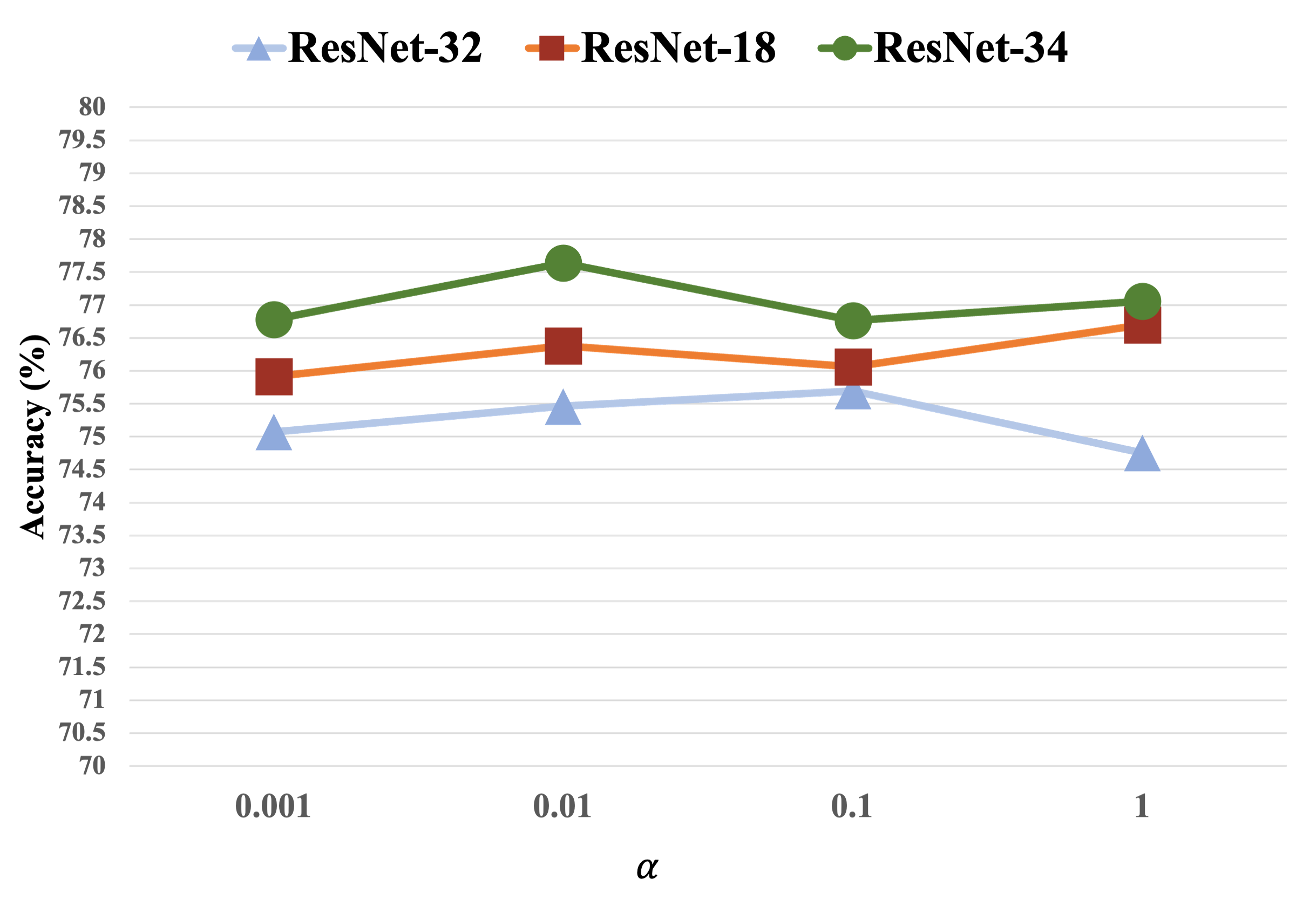
(a)

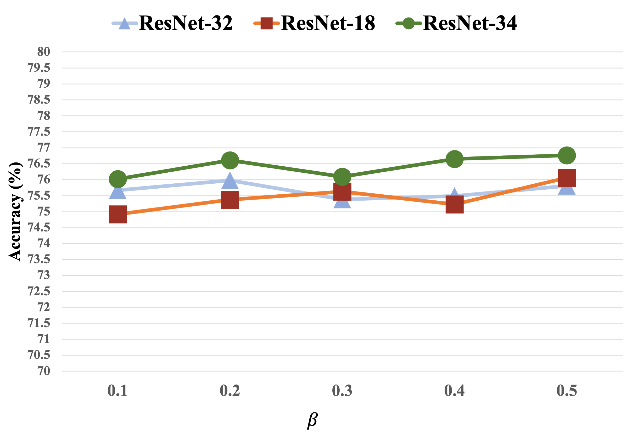
(b)

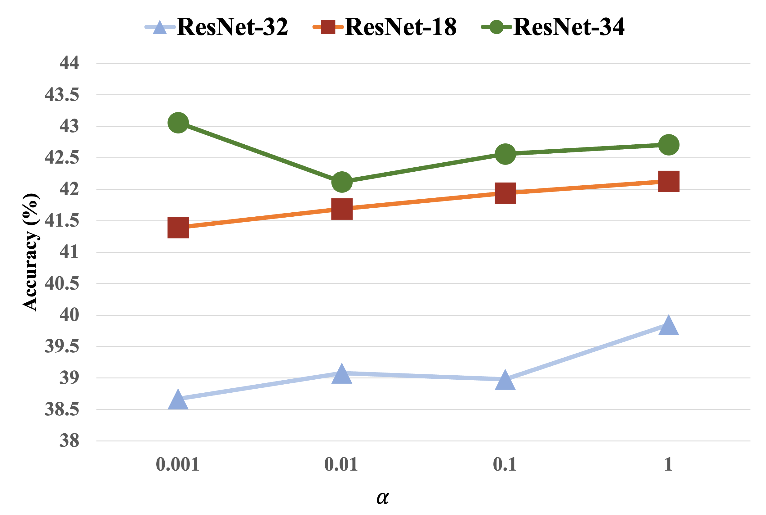
(c)

(d)

Figure 3: The influence of hyper-parameters with different values on simulated CIFAR-10 and CIFAR-100 under the imbalance ratio $100$ and noise rate $0.2$. Subfigures (a) and (c) present the results on noisy and imbalanced CIFAR-10 and CIFAR-100 under different values of $\alpha$. Additionally, subfigures (b) and (d) show the results on noisy and imbalanced CIFAR-10 and CIFAR-100 under different values of $\beta$.

B.3 Representation Visualizations

Recall that RCAL handles noisy labels on long-tailed data based on representation calibration. Here, we visualize achieved representations to demonstrate the effectiveness of the proposed method. To avoid dense figures, we visualize the representations of data points belonging to tail classes. The results are presented in Figure 4. As can be seen, RCAL can obtain more robust representations and therefore better classification performance.

– Training ($\rho=100,\eta=0.2$) –

– Test ($\rho=100,\eta=0.2$) –

– Training ($\rho=100,\eta=0.4$) –

– Test ($\rho=100,\eta=0.4$) –

– ERM –

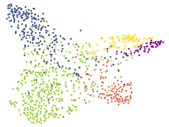
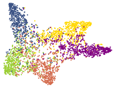
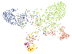
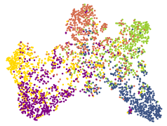
– RCAL –

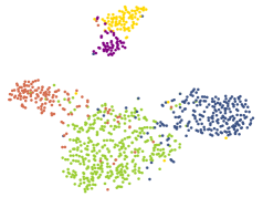
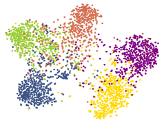
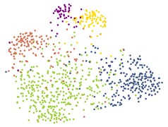
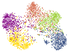
Figure 4: t-SNE visualization [54] of representations for simulated CIFAR-10 images.

Appendix C Details of Baselines

Below, we introduce the exploited baselines.

• ERM. Using the standard Cross Entropy (CE) loss, the network is simply trained on noisy and imbalanced datasets.

Methods for long-tailed distributions: 

• LDAM [6]. This work designs a label-distribution-aware loss function at the class level, which finds the best trade-off between per-class margins.

• LDAM-DRW [6]. To overcome the issues brought by re-weighting or re-sampling, a deferred re-balancing training schedule is applied with the LDAM loss. It first trains deep networks with all examples using the LDAM loss with the same weights and then deploys a re-weighted LDAM loss to weigh up the minority classes’ losses.

• CRT [27]. This work claims that data imbalance will not affect the acquisition of high-quality representations, while the strong long-tailed recognition can be achieved by adjusting only the classifier. The learning process is decoupled into representation learning and classifier learning. Representation learning can be performed by different sampling strategies. CRT is to re-train the classifier with class-balanced sampling.

• NCM [27]. Compared to CRT, NCM is to learn the classifier by computing the mean features representation for each class and then performing the nearest neighbor search.

• MiSLAS [83].

Methods for learning with noisy labels: 

• Co-teaching [18]. Two networks are exploited to handle noisy labels simultaneously, which select underlying clean examples for peer networks.

• CDR [63]. Inspired by the lottery ticket hypothesis, this work divides all parameters into critical and non-critical ones. Different types of parameters would perform different update rules to enhance the memorization effect and improve the robustness.

• Sel-CL+ [34]. To learn robust representations, this paper extends supervised contrastive learning by selecting confident pairs. With the learned representations, they further fine tune the classifier.

Methods for tackling noisy labels on long-tailed data: 

• HAR-DRW [5]. This work proposes a regularization technique to handle noisy labels and class-imbalanced data in a unified way. Different regularization strength is assigned to each data point, where data point with high uncertainty and low density will be assigned larger regularization strength.

• RoLT [61]. To distinguish mislabeled examples from rare examples, this paper designs a class-dependent noise detector by computing the distance to prototypes. This paper also employs semi-supervised methods to improve the robustness further.

• RoLT-DRW [61]. Compared to RoLT, a deferred re-weighting technique [6] is leveraged to favor tail classes.

References

- [1] Theodore Wilbur Anderson. An Introduction to Multivariate Statistical Analysis. Wiley-Interscience, 2003.
- [2] Barry C Arnold and Robert J Beaver. The skew-cauchy distribution. Statistics & probability letters, 49(3):285–290, 2000.
- [3] Markus M Breunig, Hans-Peter Kriegel, Raymond T Ng, and Jörg Sander. Lof: identifying density-based local outliers. In Proceedings of the 2000 ACM SIGMOD international conference on Management of data, pages 93–104, 2000.
- [4] Jonathon Byrd and Zachary Lipton. What is the effect of importance weighting in deep learning? In ICML, pages 872–881, 2019.
- [5] Kaidi Cao, Yining Chen, Junwei Lu, Nikos Arechiga, Adrien Gaidon, and Tengyu Ma. Heteroskedastic and imbalanced deep learning with adaptive regularization. In ICLR, 2020.
- [6] Kaidi Cao, Colin Wei, Adrien Gaidon, Nikos Arechiga, and Tengyu Ma. Learning imbalanced datasets with label-distribution-aware margin loss. In NeurIPS, 2019.
- [7] Pengfei Chen, Ben Ben Liao, Guangyong Chen, and Shengyu Zhang. Understanding and utilizing deep neural networks trained with noisy labels. In ICMl, pages 1062–1070, 2019.
- [8] Ting Chen, Simon Kornblith, Mohammad Norouzi, and Geoffrey Hinton. A simple framework for contrastive learning of visual representations. In ICML, pages 1597–1607, 2020.
- [9] Xinlei Chen, Haoqi Fan, Ross Girshick, and Kaiming He. Improved baselines with momentum contrastive learning. arXiv preprint arXiv:2003.04297, 2020.
- [10] De Cheng, Yixiong Ning, Nannan Wang, Xinbo Gao, Heng Yang, Yuxuan Du, Bo Han, and Tongliang Liu. Class-dependent label-noise learning with cycle-consistency regularization. In NeurIPS, 2022.
- [11] Yin Cui, Menglin Jia, Tsung-Yi Lin, Yang Song, and Serge Belongie. Class-balanced loss based on effective number of samples. In CVPR, pages 9268–9277, 2019.
- [12] Luc Devroye, Matthieu Lerasle, Gabor Lugosi, and Roberto I Oliveira. Sub-gaussian mean estimators. 2016.
- [13] Chris Drummond, Robert C Holte, et al. C4. 5, class imbalance, and cost sensitivity: why under-sampling beats over-sampling. In Workshop on learning from imbalanced datasets II, volume 11, pages 1–8, 2003.
- [14] Torbjørn Eltoft, Taesu Kim, and Te-Won Lee. On the multivariate laplace distribution. IEEE Signal Processing Letters, 13(5):300–303, 2006.
- [15] Aritra Ghosh and Andrew Lan. Contrastive learning improves model robustness under label noise. In CVPR, pages 2703–2708, 2021.
- [16] Ian Goodfellow, Yoshua Bengio, and Aaron Courville. Deep learning. MIT press, 2016.
- [17] Guo Haixiang, Li Yijing, Jennifer Shang, Gu Mingyun, Huang Yuanyue, and Gong Bing. Learning from class-imbalanced data: Review of methods and applications. Expert systems with applications, 73:220–239, 2017.
- [18] Bo Han, Quanming Yao, Xingrui Yu, Gang Niu, Miao Xu, Weihua Hu, Ivor Tsang, and Masashi Sugiyama. Co-teaching: Robust training of deep neural networks with extremely noisy labels. In NeurIPS, 2018.
- [19] Haibo He and Edwardo A Garcia. Learning from imbalanced data. IEEE Transactions on knowledge and data engineering, 21(9):1263–1284, 2009.
- [20] Kaiming He, Haoqi Fan, Yuxin Wu, Saining Xie, and Ross Girshick. Momentum contrast for unsupervised visual representation learning. In CVPR, pages 9729–9738, 2020.
- [21] Kaiming He, Xiangyu Zhang, Shaoqing Ren, and Jian Sun. Deep residual learning for image recognition. In CVPR, pages 770–778, 2016.
- [22] Yin-Yin He, Jianxin Wu, and Xiu-Shen Wei. Distilling virtual examples for long-tailed recognition. In ICCV, pages 235–244, 2021.
- [23] Youngkyu Hong, Seungju Han, Kwanghee Choi, Seokjun Seo, Beomsu Kim, and Buru Chang. Disentangling label distribution for long-tailed visual recognition. In CVPR, pages 6626–6636, 2021.
- [24] Xinting Hu, Yi Jiang, Kaihua Tang, Jingyuan Chen, Chunyan Miao, and Hanwang Zhang. Learning to segment the tail. In CVPR, pages 14045–14054, 2020.
- [25] Lu Jiang, Zhengyuan Zhou, Thomas Leung, Li-Jia Li, and Li Fei-Fei. Mentornet: Learning data-driven curriculum for very deep neural networks on corrupted labels. In ICML, pages 2304–2313, 2018.
- [26] Shenwang Jiang, Jianan Li, Ying Wang, Bo Huang, Zhang Zhang, and Tingfa Xu. Delving into sample loss curve to embrace noisy and imbalanced data. In AAAI, pages 7024–7032, 2022.
- [27] Bingyi Kang, Saining Xie, Marcus Rohrbach, Zhicheng Yan, Albert Gordo, Jiashi Feng, and Yannis Kalantidis. Decoupling representation and classifier for long-tailed recognition. In ICLR, 2019.
- [28] Shyamgopal Karthik, Jérome Revaud, and Boris Chidlovskii. Learning from long-tailed data with noisy labels. arXiv preprint arXiv:2108.11096, 2021.
- [29] Alex Krizhevsky, Geoffrey Hinton, et al. Learning multiple layers of features from tiny images. 2009.
- [30] Yann LeCun, Yoshua Bengio, and Geoffrey Hinton. Deep learning. nature, 521(7553):436–444, 2015.
- [31] Bo Li, Yongqiang Yao, Jingru Tan, Gang Zhang, Fengwei Yu, Jianwei Lu, and Ye Luo. Equalized focal loss for dense long-tailed object detection. In CVPR, pages 6990–6999, 2022.
- [32] Junnan Li, Richard Socher, and Steven CH Hoi. Dividemix: Learning with noisy labels as semi-supervised learning. In ICLR, 2020.
- [33] Junnan Li, Yongkang Wong, Qi Zhao, and Mohan S Kankanhalli. Learning to learn from noisy labeled data. In CVPR, pages 5051–5059, 2019.
- [34] Shikun Li, Xiaobo Xia, Shiming Ge, and Tongliang Liu. Selective-supervised contrastive learning with noisy labels. In CVPR, pages 316–325, 2022.
- [35] Shikun Li, Xiaobo Xia, Hansong Zhang, Yibing Zhan, Shiming Ge, and Tongliang Liu. Estimating noise transition matrix with label correlations for noisy multi-label learning. In NeurIPS, pages 24184–24198, 2022.
- [36] Wen Li, Limin Wang, Wei Li, Eirikur Agustsson, and Luc Van Gool. Webvision database: Visual learning and understanding from web data. arXiv preprint arXiv:1708.02862, 2017.
- [37] Kevin J Liang, Samrudhdhi B Rangrej, Vladan Petrovic, and Tal Hassner. Few-shot learning with noisy labels. In CVPR, pages 9089–9098, 2022.
- [38] Tsung-Yi Lin, Priya Goyal, Ross Girshick, Kaiming He, and Piotr Dollár. Focal loss for dense object detection. In CVPR, pages 2980–2988, 2017.
- [39] Bo Liu, Haoxiang Li, Hao Kang, Gang Hua, and Nuno Vasconcelos. Gistnet: a geometric structure transfer network for long-tailed recognition. In ICCV, pages 8209–8218, 2021.
- [40] Hong Liu, Jeff Z HaoChen, Adrien Gaidon, and Tengyu Ma. Self-supervised learning is more robust to dataset imbalance. In ICLR, 2021.
- [41] Sheng Liu, Kangning Liu, Weicheng Zhu, Yiqiu Shen, and Carlos Fernandez-Granda. Adaptive early-learning correction for segmentation from noisy annotations. In CVPR, pages 2606–2616, 2022.
- [42] Sheng Liu, Jonathan Niles-Weed, Narges Razavian, and Carlos Fernandez-Granda. Early-learning regularization prevents memorization of noisy labels. In NeurIPS, pages 20331–20342, 2020.
- [43] Tongliang Liu and Dacheng Tao. Classification with noisy labels by importance reweighting. IEEE Transactions on pattern analysis and machine intelligence, 38(3):447–461, 2015.
- [44] Xingjun Ma, Hanxun Huang, Yisen Wang, Simone Romano, Sarah Erfani, and James Bailey. Normalized loss functions for deep learning with noisy labels. In ICML, pages 6543–6553, 2020.
- [45] Xingjun Ma, Yisen Wang, Michael E Houle, Shuo Zhou, Sarah Erfani, Shutao Xia, Sudanthi Wijewickrema, and James Bailey. Dimensionality-driven learning with noisy labels. In ICML, pages 3355–3364, 2018.
- [46] Dhruv Mahajan, Ross Girshick, Vignesh Ramanathan, Kaiming He, Manohar Paluri, Yixuan Li, Ashwin Bharambe, and Laurens Van Der Maaten. Exploring the limits of weakly supervised pretraining. In ECCV, pages 181–196, 2018.
- [47] Deep Patel and PS Sastry. Adaptive sample selection for robust learning under label noise. In WACV, pages 3932–3942, 2023.
- [48] Giorgio Patrini, Alessandro Rozza, Aditya Krishna Menon, Richard Nock, and Lizhen Qu. Making deep neural networks robust to label noise: A loss correction approach. In CVPR, pages 1944–1952, 2017.
- [49] Junran Peng, Xingyuan Bu, Ming Sun, Zhaoxiang Zhang, Tieniu Tan, and Junjie Yan. Large-scale object detection in the wild from imbalanced multi-labels. In CVPR, pages 9709–9718, 2020.
- [50] Mengye Ren, Wenyuan Zeng, Bin Yang, and Raquel Urtasun. Learning to reweight examples for robust deep learning. In ICML, pages 4334–4343, 2018.
- [51] Li Shen, Zhouchen Lin, and Qingming Huang. Relay backpropagation for effective learning of deep convolutional neural networks. In ECCV, pages 467–482, 2016.
- [52] Jun Shu, Qi Xie, Lixuan Yi, Qian Zhao, Sanping Zhou, Zongben Xu, and Deyu Meng. Meta-weight-net: Learning an explicit mapping for sample weighting. In NeurIPS, 2019.
- [53] Daiki Tanaka, Daiki Ikami, Toshihiko Yamasaki, and Kiyoharu Aizawa. Joint optimization framework for learning with noisy labels. In CVPR, pages 5552–5560, 2018.
- [54] Laurens Van der Maaten and Geoffrey Hinton. Visualizing data using t-sne. Journal of machine learning research, 9(11), 2008.
- [55] Chaozheng Wang, Shuzheng Gao, Cuiyun Gao, Pengyun Wang, Wenjie Pei, Lujia Pan, and Zenglin Xu. Label-aware distribution calibration for long-tailed classification. arXiv preprint arXiv:2111.04901, 2021.
- [56] Jiaqi Wang, Wenwei Zhang, Yuhang Zang, Yuhang Cao, Jiangmiao Pang, Tao Gong, Kai Chen, Ziwei Liu, Chen Change Loy, and Dahua Lin. Seesaw loss for long-tailed instance segmentation. In CVPR, pages 9695–9704, 2021.
- [57] Tong Wang, Yousong Zhu, Chaoyang Zhao, Wei Zeng, Jinqiao Wang, and Ming Tang. Adaptive class suppression loss for long-tail object detection. In CVPR, pages 3103–3112, 2021.
- [58] Yisen Wang, Xingjun Ma, Zaiyi Chen, Yuan Luo, Jinfeng Yi, and James Bailey. Symmetric cross entropy for robust learning with noisy labels. In ICCV, pages 322–330, 2019.
- [59] Yikai Wang, Xinwei Sun, and Yanwei Fu. Scalable penalized regression for noise detection in learning with noisy labels. In CVPR, pages 346–355, 2022.
- [60] Jiaheng Wei and Yang Liu. When optimizing -divergence is robust with label noise. In ICLR, 2021.
- [61] Tong Wei, Jiang-Xin Shi, Wei-Wei Tu, and Yu-Feng Li. Robust long-tailed learning under label noise. arXiv preprint arXiv:2108.11569, 2021.
- [62] Songhua Wu, Xiaobo Xia, Tongliang Liu, Bo Han, Mingming Gong, Nannan Wang, Haifeng Liu, and Gang Niu. Class2simi: A noise reduction perspective on learning with noisy labels. In ICML, pages 11285–11295, 2021.
- [63] Xiaobo Xia, Tongliang Liu, Bo Han, Chen Gong, Nannan Wang, Zongyuan Ge, and Yi Chang. Robust early-learning: Hindering the memorization of noisy labels. In ICLR, 2021.
- [64] Xiaobo Xia, Tongliang Liu, Bo Han, Mingming Gong, Jun Yu, Gang Niu, and Masashi Sugiyama. Sample selection with uncertainty of losses for learning with noisy labels. In ICLR, 2022.
- [65] Xiaobo Xia, Tongliang Liu, Bo Han, Nannan Wang, Mingming Gong, Haifeng Liu, Gang Niu, Dacheng Tao, and Masashi Sugiyama. Part-dependent label noise: Towards instance-dependent label noise. In NeurIPS, pages 7597–7610, 2020.
- [66] Xiaobo Xia, Tongliang Liu, Nannan Wang, Bo Han, Chen Gong, Gang Niu, and Masashi Sugiyama. Are anchor points really indispensable in label-noise learning? In NeurIPS, 2019.
- [67] Yongqin Xian, Tobias Lorenz, Bernt Schiele, and Zeynep Akata. Feature generating networks for zero-shot learning. In CVPR, pages 5542–5551, 2018.
- [68] Tong Xiao, Tian Xia, Yi Yang, Chang Huang, and Xiaogang Wang. Learning from massive noisy labeled data for image classification. In CVPR, pages 2691–2699, 2015.
- [69] Yihao Xue, Kyle Whitecross, and Baharan Mirzasoleiman. Investigating why contrastive learning benefits robustness against label noise. In ICML, 2022.
- [70] Shuo Yang, Lu Liu, and Min Xu. Free lunch for few-shot learning: Distribution calibration. In ICLR, 2021.
- [71] Quanming Yao, Hansi Yang, Bo Han, Gang Niu, and James Kwok. Searching to exploit memorization effect in learning from corrupted labels. In ICML, 2020.
- [72] Yu Yao, Tongliang Liu, Bo Han, Mingming Gong, Jiankang Deng, Gang Niu, and Masashi Sugiyama. Dual t: Reducing estimation error for transition matrix in label-noise learning. In NeurIPS, pages 7260–7271, 2020.
- [73] Kun Yi and Jianxin Wu. Probabilistic end-to-end noise correction for learning with noisy labels. In CVPR, pages 7017–7025, 2019.
- [74] Hongyi Zhang, Moustapha Cisse, Yann N Dauphin, and David Lopez-Paz. mixup: Beyond empirical risk minimization. In ICLR, 2017.
- [75] Manyi Zhang, Yuxin Ren, Zihao Wang, and Chun Yuan. Tackling instance-dependent label noise with dynamic distribution calibration. In ACMMM, pages 4635–4644, 2022.
- [76] Songyang Zhang, Zeming Li, Shipeng Yan, Xuming He, and Jian Sun. Distribution alignment: A unified framework for long-tail visual recognition. In CVPR, pages 2361–2370, 2021.
- [77] Yiliang Zhang, Yang Lu, Bo Han, Yiu-ming Cheung, and Hanzi Wang. Combating noisy-labeled and imbalanced data by two stage bi-dimensional sample selection. arXiv preprint arXiv:2208.09833, 2022.
- [78] Yikai Zhang, Songzhu Zheng, Pengxiang Wu, Mayank Goswami, and Chao Chen. Learning with feature-dependent label noise: A progressive approach. In ICLR, 2021.
- [79] Zhilu Zhang and Mert Sabuncu. Generalized cross entropy loss for training deep neural networks with noisy labels. In NeurIPS, 2018.
- [80] Yan Zhao, Weicong Chen, Xu Tan, Kai Huang, and Jihong Zhu. Adaptive logit adjustment loss for long-tailed visual recognition. In AAAI, pages 3472–3480, 2022.
- [81] Evgenii Zheltonozhskii, Chaim Baskin, Avi Mendelson, Alex M Bronstein, and Or Litany. Contrast to divide: Self-supervised pre-training for learning with noisy labels. In WACV, pages 1657–1667, 2022.
- [82] Songzhu Zheng, Pengxiang Wu, Aman Goswami, Mayank Goswami, Dimitris Metaxas, and Chao Chen. Error-bounded correction of noisy labels. In ICML, pages 11447–11457, 2020.
- [83] Zhisheng Zhong, Jiequan Cui, Shu Liu, and Jiaya Jia. Improving calibration for long-tailed recognition. In CVPR, pages 16489–16498, 2021.