AI-KD: Adversarial learning and Implicit regularization for self-Knowledge Distillation

Abstract

We present a novel adversarial penalized self-knowledge distillation method, named adversarial learning and implicit regularization for self-knowledge distillation (AI-KD), which regularizes the training procedure by adversarial learning and implicit distillations. Our model not only distills the deterministic and progressive knowledge which are from the pre-trained and previous epoch predictive probabilities but also transfers the knowledge of the deterministic predictive distributions using adversarial learning. The motivation is that the self-knowledge distillation methods regularize the predictive probabilities with soft targets, but the exact distributions may be hard to predict. Our method deploys a discriminator to distinguish the distributions between the pre-trained and student models while the student model is trained to fool the discriminator in the trained procedure. Thus, the student model not only can learn the pre-trained model’s predictive probabilities but also align the distributions between the pre-trained and student models. We demonstrate the effectiveness of the proposed method with network architectures on multiple datasets and show the proposed method achieves better performance than state-of-the-art methods.

1 Introduction

Deep neural networks (DNNs) are leading outstanding breakthroughs in computer vision and various tasks. For better performance, the quantity of training data is increased, and network architecture is not only intricated but also has numerous parameters. However, the cumbersome networks for handling large datasets may incur the overfitting problem, leading to hurt generalization. The regularization techniques alleviate these issues and are adopted essentially to train the networks effectively, such as dropout [1], batch normalization [2], and label smoothing [3, 4].

Knowledge distillation (KD) [5] aims to efficient model compression to transfer knowledge from the larger deep teacher network into the lightweight student network. The method usually utilizes the Kullback-Leibler (KL) divergence between the softened probability distributions of the teacher and the student network with the temperature scaling parameter. However, KD has an inherent drawback which is a drop in accuracy by transferring compacted information, so it is not always the effectual approach where there are significant gaps in the quantity of parameters between the teacher and the student models and where the models are heterogeneously different. Also, it is hard to tell which intermediate features of teacher are the best selection and where to transfer on features of the student. On the other hands, the multiple selected features may not represent better knowledge than a single feature of the layer. Thus, various approaches apply neural architecture search and meta-learning to handle the selection, which features and intermediate layers of the teacher and the student models, for better knowledge transfer. In this manner, Jang and Shin [6], and Mirzadeh and Ghasemzadeh [7] proposed utilizing meta networks and bridge models to alleviate differences from the network models, respectively.

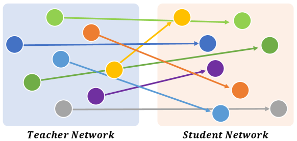
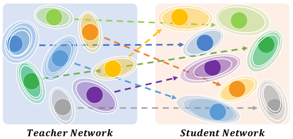
(a) Conventional Knowledge Distillation	(b) Adversarial Implicit Knowledge Distillation

Figure 1: Concept comparison with conventional knowledge distillation methods. Each point denotes a latent vector represented from the different input data. (a) The solid line indicates that the conventional knowledge distillation is trained to minimize the distance between the latent vector point in the teacher network and the corresponding latent vector point in the student network. (b) The dashed line indicates that AI-KD is trained to minimize the distance between the distribution of the latent vectors in the teacher network and the distribution of the corresponding latent vectors in the student network.

While, Self-knowledge distillation (Self-KD) trains the network itself as a teacher network, aims to regularize the model to avoid overfitting using only the student model. In other words, Self-KD does not consider compactivity since transferring knowledge between homogeneous networks. And the method, as one of regularization techniques, can focus on alleviating the overfitting issue and improving generalization performance efficiently. The feature-based Self-KD approaches are also effective generalization techniques since the features have abundant representative capacity. However, most methods minimize the distance between each feature using $L2$ distance or cosine similarity, which should require additional modifications of networks. The logit-based Self-KDs are intuitive, do not require any model adjustment and considering which to where since the capacity of logit is explicit. Given the limited capacity, the methods tend to hurdle securing generality depending on various datasets. However, recent proposed logit-based methods overcome the capacity issues and present outperformed generalization than feature-based approaches. Teacher-free KD (TF-KD) [8] revealed that a powerful and well-trained teacher is not essential component for KD. Instead, the pre-trained student model as the teacher model transfer could utilize to distill knowledge, and verified their argument by presenting comparable performance on TF-KD to conventional KD. Progressive Self-KD (PS-KD) [9] distills knowledge by generating the soft labels using historically, previous predictive distributions at the last epoch. However, the these methods regularized the predictive probabilities with soft targets, while the exact distributions may be hard to predict, as shown in Figure 1(a). It means that the methods are focused on trying to mimic the predictive probability information by the other network as the direct aligning method, which loses the chance to deem reducing distributional differences between the models.

In this paper, we propose a novel logit-based Self-KD method via adversarial learning, coined adversarial learning and implicit regularization for self-knowledge distillation (AI-KD). The proposed method learns implicitly distilled deterministic and progressive knowledge from the pre-trained model and the previous epoch student model, and aligns the distributions of the student model to the distributions of the pre-trained using adversarial learning, as shown in Figure 1 (b). The pre-trained model is the baseline of the dataset and is trained from scratch following standard training parameters. The method distills knowledge by considering the probability distribution of two networks so that align not directly, and it leads to better model generalization. To verify the generalization effectiveness, we evaluate the proposed method using ResNet [10, 11] and DenseNet [12] on coarse and fine-grained datasets. In addition, we demonstrate compatibility with recent image augmentation methods to provide broad applicability with other regularization techniques.

The main contributions of the proposed method can be summarized as follows.

• We propose a novel adversarial Self-KD, named AI-KD, between the pre-trained and the student models. Our method provides the student model can align to the predictive probability distributions of the pre-trained models by adversarial learning.

• For training stability, AI-KD distills implicit knowledge of deterministic and progressive from the pre-trained and the previous epoch model, respectively.

• In the experiments, AI-KD is evaluated to show the performance of the generalization on various public datasets. We also verify the compatibility of AI-KD with the data augmentations.

The rest of the paper is organized as follows. Section 2 introduces related work. Section 3 provides the details of the proposed method. Section 4 presents qualitative and quantitative experimental results with a variety of network architectures on the multiple datasets, including coarse datasets and fine-grained dataset. Finally, Section 5 concludes the paper and addresses future works.

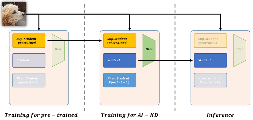
Figure 2: The overall framework of AI-KD. Training models through AI-KD have a two-step process. The first phase is training the pre-trained model, which is learned with standard parameters. The pre-trained model is treated to baseline and utilized as the superior student model in the next phase. Then the second phase is training the student model via AI-KD. In the inference phase, the well-trained student model only is utilized.

2 Related Works

2.1 Self-knowledge distillation

Self-KD is trained using the same network as teacher and student. And it leads to affecting the improving generalization performance rather model compression. One of the Self-KD approaches uses multiple auxiliary heads and requires a lot of network architecture modifications. They lead to increasing its difficulty for deployments, such as Be your own teacher (BYOT) [13] and Harmonized dense KD (HD-KD) [14]. Another approach is utilizing the input-based method. Data-distortion guided Self-KD (DDGSD) [15] focuses on constraining consistent outputs across an image distorted differently. Yun and Shin [16] proposed a class-wise Self-KD (CS-KD) that distills the knowledge of a model itself to force the predictive distributions between different samples in the same class by minimizing KL divergence. PS-KD [9], Memory-replay KD (Mr-KD) [17], Self distillation from last mini-batch (DLB) [18], and Snapshot [19] proposed progressive knowledge distillation methods that distill the knowledge of a model itself as a virtual teacher by utilizing the past predictive distributions at the last epoch, the last minibatch, and the last iteration, respectively. Born again neural networks (BANs) [20] train a student network to use as a teacher for the next generations, iteratively. In these manners, it performs multiple generations of ensembled Self-KD. In contrast, [8] proposed the TF-KD that uses a pre-trained student network as a teacher network for a single generation. This method aligns directly between the teacher and student model so that the student model only mimics the teacher model.

2.2 Adversarial learning

Generative adversarial network (GAN) [21] is a min-max game between a generator and a discriminator to to approximate the probability distributions and generate real-like data. The goal of the generator is to deceive the discriminator into fake determining the results as the real samples. The generator is trained to generate the real data distribution, while the discriminator is trained to distinguish the real samples from the fake samples generated by the generator. There are various works proposed to overcome the well-known issue in GAN, which is unstable training procedure due to the gradient vanishing problem in training procedure. Wasserstein GAN with gradient penalty (WGAN-GP) [22] alleviates the issue using Earth-Mover’s distance and adopt the weight clipping method for training stability.

Recently, adversarial learning has been studied to utilize for KD. One approach addressed training a generator to synthesize input images by the teacher’s features, and then the images are utilized to transfer the knowledge to the student network [23, 24, 25]. Online adversarial feature map distillation (AFD) [26], meanwhile, has been proposed to utilize adversarial training to distill knowledge using two or three different networks at each feature extractor. As the generator of GAN, the feature extractors are trained to deceive the discriminators. Xu and Li [27] proposed a contrastive adversarial KD with a designed two-stage framework: one is for feature distillation using adversarial and contrastive learning and another is for KD.

3 Methodology

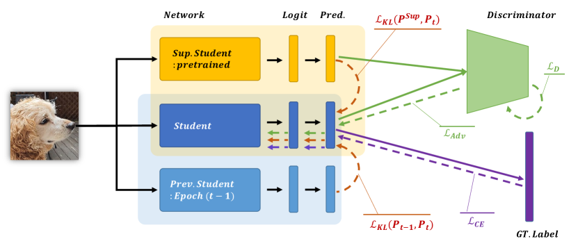
Figure 3: The overall losses of AI-KD. The student model is trained implicitly distilled knowledge from the superior pre-trained and previous student models. Through adversarial learning, the student is aligned to the distributions of the superior pre-trained model.

3.1 Overall framework

AI-KD utilizes three same-size network architectures but different objectives, which are the pre-trained model, the student model, and the previous student model. The pre-trained model learns with the corresponding dataset using standard training parameters, not employing the ImageNet pre-trained model. So, we should acquire the corresponding pre-trained model from scratch to train through our proposed method properly. For that reason, AI-KD has a two-phase training procedure, as shown in Figure 2. The first step is acquiring a pre-trained model. The model architecture and training parameters(e.g., learning rate, weight decay, batch size, and standard data augmentation approaches) of the pre-trained model are identical to the student model. The acquired pre-trained model is utilized as named superior student model to align direct output distributions of the student model to the pre-trained model. The acquired pre-trained model is utilized as named superior student model to guide mimicking output distributions of the student model to the pre-trained model in the next phase. Then the second step is training the student model to utilize two different models, which are the pre-trained model and the old student model from the previous epoch. In the inference phase, the pre-trained and previous student models are not activated, and the well-trained student model is only utilized.

The discriminator aims to distinguish whether the output distributions are from the student model or from the pre-trained model. For that reason, the discriminator requires as input one-dimensional and consists of stacking two different sizes of fully-connected layers. The activation function of the discriminator is Leaky ReLU. The single one-dimensional batch normalization technique is employed to better utilizing the discriminator. The batch normalization and the activation function are placed between fully-connected layers as Fully Connected Layer-1D Batch Normalization-LeakyReLU-Fully Connected Layer. The discriminator is employed only in the second phase and is not utilized in the acquiring pre-trained model phase and the inference phase.

3.2 Objective of learning via AI-KD losses

In this work, we focus on fully-supervised classification tasks. The input data and the corresponding ground-truth labels are denoted as $x\in X$ and $y\in Y=\{1,\dots,C\}$, respectively. Given a student model $S$, $S$ outputs posterior predictive distribution of each input using a softmax classifier.

$$p_{i}(x;\tau)=\frac{exp(z_{i}(x)/\tau)}{\sum_{i=1}^{C}exp(z_{i}(x)/\tau)}$$ (1)

where $z_{i}$ is the logit of the model for class $i$, and $\tau>0$ is the temperature scaling parameter to soften $p_{i}$ for better distillation.

In conventional KD, the loss for training the student model is given by

$$\mathcal{L}_{KD}=(1-\alpha)\mathcal{H}(q,p^{S}(x))+\alpha{\tau}^{2}\mathcal{H}(p^{T}(x;\tau),p^{S}(x;\tau))$$ (2)

where $\mathcal{H}(\cdot,\cdot)$ indicates the standard cross-entropy, $\alpha$ is the balancing hyper-parameter, and $p^{S}$ and $p^{T}$ are output probabilities of a student and teacher network, respectively. $q$ denotes $C$-dimensional one-hot of $y$.

Let $D_{KL}$ denotes the KL divergence, and $\mathcal{H}(p^{T},p^{S})=D_{KL}(p^{T},p^{S})-\mathcal{H}(p^{T})$, then we can reformulate Equation 2 as

$$\mathcal{L}_{KD} =(1-\alpha)\mathcal{H}(y,p^{S}(x))$$ (3)

$$~{}~{}~{}+\alpha{\tau}^{2}D_{KL}(p^{T}(x;\tau),p^{S}(x;\tau))-\alpha{\tau}^{2}\mathcal{H}(p^{T}(x;\tau))$$

$$=(1-\alpha)\mathcal{H}(y,p^{S}(x))+\alpha{\tau}^{2}D_{KL}(p^{T}(x;\tau),p^{S}(x;\tau))$$

where $p^{T}$ from the pre-trained model should have deterministic probability distributions, then the entropy $\mathcal{H}(\cdot)$ is treated as a constant for the fixed model and can be ignored.

From Equation 3, we separate the $D_{KL}$ into two terms for distilling deterministic and progressive knowledge from different models. And, as depicted in Figure 3, the overall architecture of AI-KD consists of two different methods: a deterministic and progressive knowledge distillation method and an adversarial learning method to align distributions between pre-trained and student models. The student network learns different knowledge using two homogeneous networks of deterministic probability distributions which are the pre-trained and the previous epoch model. We define three different networks: a superior pre-trained student model $S^{Sup}$, a student model $S_{t}$, and a previous epoch $(t-1)^{th}$ student model $S_{t-1}$. The output of the superior pre-trained model, $p^{Sup}$, and the output of the previous epoch student model, $p_{t-1}$, are used to distill implicit knowledge to the student model by penalizing the output of the student model, $p_{t}$.

The model is not from the ImageNet dataset; instead is the baseline of each dataset and is trained from scratch following the standard training parameters. The role of $S^{Sup}$ is that as a good guide and teacher, the superior model guides the student model to improve performance. In this sense, the loss function for distillation of $S^{Sup}$ is named guide, $\mathcal{L}_{G}$ and aims that $S$ directly mimics the logits of $S^{Sup}$. $\mathcal{L}_{G}$ can be written as

$$\mathcal{L}_{G}={\tau_{G}}^{2}~{}D_{KL}(p^{Sup}(x;\tau_{G}),~{}p_{t}(x;\tau_{G}))$$ (4)

$L_{G}$ may induce rapid weight variation in epochs, leading to degraded performance. To prevent the performance degradation and unsteady learning, the student model is available to acquire progressive information from the previous knowledge. We empirically observed that the $t-1^{th}$ epoch model could provide effective knowledge distilled for training progressively. The loss function of learning from previous predictions is coined $L_{P}$ and affects regularization by logit smoothing. In this manner, $L_{P}$ can be written as

$$\mathcal{L}_{P}={\tau_{P}}^{2}~{}D_{KL}(p_{t-1}(x;\tau_{P}),~{}p_{t}(x;\tau_{P}))$$ (5)

Although the student model is regularized by $L_{G}$ and $L_{P}$, the predictive logits of the student model can just be overfitting to the logits of the pre-trained model. To prevent overfitting, AI-KD employs an adversarial learning method utilizing a discriminator $D$ that is composed of two fully-connected layers to distinguish $p^{Sup}$ and $p_{t}$. The goal of the proposed method is to align the predictive distributions of the student model to the predictive distributions of the pre-trained model. By adopting the adversarial learning method, the student model is trained to fool the discriminator. A well-trained discriminator helps the student model to be trained to generalize the predictive distributions to the pre-trained model. Motivated by WGAN-GP [22], $\mathcal{L}_{D}$ is defined as a critic loss that scores between the pre-trained model and the student model.

$$\mathcal{L}_{D} =\mathbb{E}_{x\sim p_{t}(x)}[D(S_{t}(x))]-\mathbb{E}_{x\sim p^{Sup}(x)}[D(S^{Sup}(x))]$$ (6)

$$~{}~{}~{}+\lambda\mathbb{E}_{\hat{x}\sim p_{\hat{x}}}[(||\nabla_{\hat{x}}D(\hat{x})||_{2}-1)^{2}]$$

where the last term indicates gradient penalty, and the middle term is ignored which is from the deterministic. In this manner, the adversarial loss $\mathcal{L}_{A}$ for the student model should be contrastive to $\mathcal{L}_{D}$ and aims to regularize the predictive distributions of the student model to align with the output distributions of the pre-trained model. $\mathcal{L}_{A}$ can be written as

$$\mathcal{L}_{A}=-\mathbb{E}_{x\sim p_{t}(x)}[D(S_{t}(x))]$$ (7)

In conclusion, the AI-KD loss consists of two different losses, one loss is for training the discriminator as follows to Equation 6, and another loss is for training the student model, $\mathcal{L}_{AI}$ is described as follows:

$$\mathcal{L}_{AI}=(1-{\alpha}_{P}-{\alpha}_{G})\mathcal{H}(q,p_{t})+{\alpha}_{P}\mathcal{L}_{P}+{\alpha}_{G}\mathcal{L}_{G}+\omega\mathcal{L}_{A}$$ (8)

where the coefficient $\alpha_{P}$, $\alpha_{G}$, and $\omega$ is deployed to balance the cross-entropy, KD losses by different models, and adversarial loss, respectively.

To sum up the objective of each proposed loss, the $\mathcal{L}_{G}$ guides that $S_{t}$ directly mimics the logits of $S^{Sup}$, may induce rapid weight variation in epochs, and leads to degraded performance. The previous loss, $\mathcal{L}_{P}$ affects to regularize as logit smoothing by distilling information from the previous epoch to prevent degradation. However, the overfitting issue is still inherent. To address the issue, $\mathcal{L}_{A}$ is the crucial loss function that the predictive distributions of $S_{t}$ lead to aligning with the output distributions of $S^{Sup}$.

4 Experiment results

In this section, we describe the effectiveness of our proposed method on the image classification task with network architectures on various coarse and fine-grained datasets. In Section 4.1, we first introduces the datasets and the metrics utilized to verify the performance of our proposed method. And Section 4.2 describe specific training environments and parameters. Then we confirm to compare the classification results with logit-based Self-KD state-of-the-arts methods, in Section 4.3. For a fair comparison, the hyper-parameters of comparison methods, such as CS-KD [16], TF-KD [8], and PS-KD [9], are set as reported. All the reported performances are average results over three runs of each experiment. In Section 4.4, we experiment with ablation studies and empirical analyses to confirm the effects of losses and balancing weight parameters for each loss. Lastly, we evaluate compatibility with other data augmentation techniques to confirm that AI-KD is a valid regularization method and could be employed with other approaches independently, in Section 4.5.

Table 1: The datasets to evaluate classification tasks. The coarse datasets are consisted of classifying interspecies, while the fine-grained datasets are composed of recognizing specific species.

Category	Dataset	Classes	Images
			Train	Valid
Coarse	CIFAR-100 [28]	10	50,000	10,000
	Tiny-ImageNet [28]	200	100,000	10,000
Fine-grained	CUB200-2011 [29]	200	5,994	5,794
	Stanford Dogs [30]	120	12,000	8,580
	MIT67 [31]	67	5,360	1,340
	FGVC aircraft [32]	100	6,667	3,334

Table 2: Image classification Top-1 error and F1 Score results on ResNet-18 and DenseNet-121 with various datasets. We report mean and standard deviation over three runs. The best and second-best results are indicated in bold and underlined, respectively.

Metric	Model	Method	Dataset
			CIFAR-100	Tiny ImageNet	CUB 200-2011	Stanford Dogs	MIT67	FGVC Aircraft
Top-1 Error	ResNet 18	Baseline	23.97$\pm$0.29	46.28$\pm$0.19	36.65$\pm$0.87	32.61$\pm$0.55	39.90$\pm$0.16	18.61$\pm$1.16
		CS-KD [16]	21.67$\pm$0.25	41.68$\pm$0.15	33.93$\pm$0.29	30.87$\pm$0.05	41.42$\pm$0.45	19.66$\pm$0.02
		TF-KD [8]	22.07$\pm$0.38	43.66$\pm$0.08	35.92$\pm$0.58	31.25$\pm$0.27	38.08$\pm$0.55	19.27$\pm$0.49
		PS-KD [9]	21.16$\pm$0.22	43.45$\pm$0.28	34.01$\pm$0.74	29.20$\pm$0.23	37.55$\pm$0.61	16.80$\pm$0.18
		AI-KD	19.87$\pm$0.10	41.84$\pm$0.10	29.59$\pm$0.27	28.61$\pm$0.21	36.84$\pm$0.34	15.43$\pm$0.15
	DenseNet 121	Baseline	19.71$\pm$0.37	40.38$\pm$0.14	34.69$\pm$0.09	33.19$\pm$0.80	37.59$\pm$0.62	17.71$\pm$0.17
		CS-KD [16]	21.48$\pm$0.32	38.21$\pm$0.17	30.93$\pm$0.82	28.70$\pm$0.14	41.02$\pm$1.28	17.37$\pm$0.36
		TF-KD [8]	18.90$\pm$0.22	38.46$\pm$0.36	32.95$\pm$0.65	30.41$\pm$0.29	36.42$\pm$0.66	16.71$\pm$0.40
		PS-KD [9]	18.69$\pm$0.12	38.62$\pm$0.44	34.28$\pm$0.50	30.54$\pm$0.03	35.92$\pm$0.48	16.38$\pm$0.71
		AI-KD	18.35$\pm$0.18	38.33$\pm$0.07	26.65$\pm$0.29	27.13$\pm$0.16	34.58$\pm$0.75	13.84$\pm$0.38
F1 Score Macro	ResNet 18	Baseline	0.759$\pm$0.003	0.536$\pm$0.002	0.631$\pm$0.008	0.663$\pm$0.006	0.598$\pm$0.004	0.821$\pm$0.002
		CS-KD [16]	0.781$\pm$0.002	0.581$\pm$0.002	0.651$\pm$0.005	0.681$\pm$0.001	0.583$\pm$0.002	0.804$\pm$0.000
		TF-KD [8]	0.779$\pm$0.004	0.563$\pm$0.001	0.638$\pm$0.006	0.678$\pm$0.003	0.621$\pm$0.007	0.807$\pm$0.005
		PS-KD [9]	0.788$\pm$0.002	0.560$\pm$0.003	0.657$\pm$0.007	0.697$\pm$0.002	0.623$\pm$0.004	0.831$\pm$0.002
		AI-KD	0.801$\pm$0.001	0.581$\pm$0.002	0.701$\pm$0.003	0.703$\pm$0.002	0.624$\pm$0.004	0.845$\pm$0.001
	DenseNet 121	Baseline	0.802$\pm$0.004	0.594$\pm$0.001	0.650$\pm$0.007	0.656$\pm$0.007	0.620$\pm$0.008	0.824$\pm$0.002
		CS-KD [16]	0.784$\pm$0.005	0.616$\pm$0.001	0.689$\pm$0.007	0.703$\pm$0.002	0.588$\pm$0.014	0.826$\pm$0.005
		TF-KD [8]	0.811$\pm$0.002	0.617$\pm$0.002	0.668$\pm$0.007	0.686$\pm$0.004	0.633$\pm$0.006	0.833$\pm$0.005
		PS-KD [9]	0.813$\pm$0.001	0.609$\pm$0.005	0.655$\pm$0.005	0.681$\pm$0.001	0.635$\pm$0.004	0.835$\pm$0.008
		AI-KD	0.816$\pm$0.002	0.617$\pm$0.002	0.730$\pm$0.004	0.714$\pm$0.006	0.649$\pm$0.008	0.861$\pm$0.004

4.1 Datasets and evaluation metrics

Datasets

We evaluate the proposed method for image classification performance using a variety of the coarse and the fine-grained datasets, as shown in Table 1. The fine-grained datasets are composed for recognizing specific species, e.g., canines, indoor scenes, vehicles, and birds. While the coarse datasets are intended to evaluate classifying interspecies objects. The proposed method is evaluated on the coarse datasets, CIFAR-100 [28] and Tiny-ImageNet, using PreAct ResNet-18 [11] and DenseNet-121 [12]. For the fine-grained datasets which are CUB200-2011 [29], Stanford Dogs [30], MIT67 [31], and FGVC aircraft [32], we utilize ResNet-18 [10] and DenseNet-121.

Metrics

The Top-$\mathcal{K}$ error rate is the fraction of evaluation samples that from the logit results, the correct label does not include in the Top-$\mathcal{K}$ confidences. We utilize the Top-1 and Top-5 error rates to evaluate the regularization performance of AI-KD. F1-score is described as $2\frac{PR}{P+R}$, where $\mathcal{P}$ and $\mathcal{R}$ indicate precision and recall. The metric represents the balance between precision and recall and the score is widely used for comparing imbalanced datasets. In addition, we measure calibration effects using expected calibration error (ECE) [33, 34]. ECE approximates the expected difference between the average confidence and the accuracy.

4.2 Implementation details

All experiments were performed on NVIDIA RTX 2080 Ti system with PyTorch. We utilize the standard augmentation techniques, such as random crop after padding and random horizontal flip. All the experiments are trained for 300 epochs using SGD with the Nesterov momentum and weight decay, 0.9 and 0.0005, respectively. The initial learning rate is 0.1 and is decayed by a factor of 0.1 at epochs 150 and 225. We utilize different batch sizes depending on the dataset type, 128 for the coarse datasets and 32 for the fine-grained datasets.

In the proposed AI-KD, the goal of the discriminator network is to distinguish the outputs between the superior pre-trained model and the student model. In this manner, the student model is trained to mimic the superior model, and the probability distributions of the student model also try to align with the probability distributions of the superior model. The discriminative network requires input one-dimensional simple information that is the logits from the student and the superior models. In this sense, we propose a light series of fully connected (FC) layer-1D Batch Normalization-LeakyReLU-FC layer. These two FC layers have different dimensions and are denoted as $FC_{1}$ and $FC_{2}$. And the layers have 64 and 32 output features, respectively. The optimizer of the discriminator is Adam and the initial learning rate is 0.0001. For gradient penalty, we utilize that the weight is set to 10.

Table 3: The performance using Top-5 error rates, and expected calibration error (ECE) [34] on ResNet-18 and DenseNet-121 with various datasets. We report mean and standard deviation over three runs. The best and second-best results are indicated in bold and underlined, respectively. TS denotes the temperature scaling for calibration.

Metric	Model	Method	Dataset
			CIFAR-100	Tiny ImageNet	CUB 200-2011	Stanford Dogs	MIT67	FGVC Aircraft
Top-5 Error	ResNet 18	Baseline	6.80$\pm$0.02	22.61$\pm$0.20	15.33$\pm$0.27	9.67$\pm$0.53	16.19$\pm$0.27	4.94$\pm$0.23
		CS-KD [16]	5.63$\pm$0.15	19.42$\pm$0.12	13.74$\pm$0.05	8.52$\pm$0.04	16.97$\pm$0.44	4.34$\pm$0.26
		TF-KD [8]	5.61$\pm$0.07	21.17$\pm$0.30	14.09$\pm$0.25	8.78$\pm$0.32	15.57$\pm$0.56	4.74$\pm$0.13
		PS-KD [9]	5.29$\pm$0.12	20.53$\pm$0.22	13.67$\pm$0.53	7.90$\pm$0.19	14.35$\pm$0.86	3.89$\pm$0.14
		AI-KD	4.81$\pm$0.04	19.87$\pm$0.21	11.47$\pm$0.23	8.17$\pm$0.06	15.55$\pm$0.37	4.06$\pm$0.15
	DenseNet 121	Baseline	4.77$\pm$0.15	17.73$\pm$0.19	12.94$\pm$0.47	8.56$\pm$0.50	14.75$\pm$0.78	4.31$\pm$0.18
		CS-KD [16]	6.67$\pm$0.08	16.82$\pm$0.21	11.36$\pm$0.38	7.23$\pm$0.19	16.52$\pm$0.80	4.06$\pm$0.11
		TF-KD [8]	4.20$\pm$0.07	16.32$\pm$0.40	11.98$\pm$0.11	7.20$\pm$0.30	12.61$\pm$0.27	3.74$\pm$0.17
		PS-KD [9]	4.06$\pm$0.11	17.01$\pm$0.30	13.18$\pm$0.34	7.76$\pm$0.15	13.18$\pm$0.34	3.59$\pm$0.08
		AI-KD	4.14$\pm$0.06	16.50$\pm$0.44	9.46$\pm$0.14	6.34$\pm$0.13	12.44$\pm$0.82	3.53$\pm$0.09
ECE	ResNet 18	Baseline	11.90	10.51	7.18	7.64	12.80	3.98
		CS-KD [16]	5.50	3.73	15.45	9.75	15.58	6.24
		TF-KD [8]	11.03	10.64	8.01	8.13	12.82	4.97
		PS-KD [9]	1.37	21.41	24.88	30.05	20.44	24.45
		AI-KD	14.10	15.00	26.43	20.41	20.29	18.74
		+ TS [34]	2.95	1.63	2.80	3.39	4.80	1.89
	DenseNet 121	Baseline	7.74	4.60	5.06	4.69	9.63	2.38
		CS-KD [16]	14.66	2.14	7.27	2.83	8.74	3.14
		TF-KD [8]	9.87	5.81	4.18	4.48	10.64	2.75
		PS-KD [9]	1.34	24.16	26.57	33.64	20.56	27.80
		AI-KD	5.11	1.89	26.66	20.14	19.26	18.20
		+ TS [34]	1.70	1.67	1.99	1.73	4.06	1.46

4.3 Comparison with State-of-the-Arts

As presented in Table 2, AI-KD shows competitive performances on coarse datasets in two network architectures. Especially on the CIFAR-100 dataset, our proposed method records $19.87\%$ Top-1 error on PreAct ResNet-18 and outperforms CS-KD, TF-KD, and PS-KD by $1.43\%$, $2.20\%$, and $1.29\%$, respectively. Also, AI-KD outperforms other state-of-the-art methods on the CIFAR-100 dataset with DenseNet-121. For the Tiny-ImageNet dataset, the proposed method achieves the second-best on ResNet and DenseNet, but the difference with the best performance is only $0.16\%$ and $0.12\%$, respectively. Most of the remarkable points are evaluated performances of fine-grained datasets. We experiment to evaluate AI-KD with four different fine-grained datasets on ResNet-18 and DenseNet-121. Our proposed method records outperforming performance in every result than other compared methods, while previous state-of-the-art methods such as CS-KD and PS-KD record the second-best performance depending on specific datasets and network architectures. In particular, on the CUB200-2011 dataset, AI-KD improves Top-1 error performance over the second-best method, CS-KD, by $4.34\%$ and $4.28\%$ on ResNet-18 and DenseNet-121, respectively. AI-KD also shows improved performances compared methods in terms of F1-score on all datasets and network architectures.

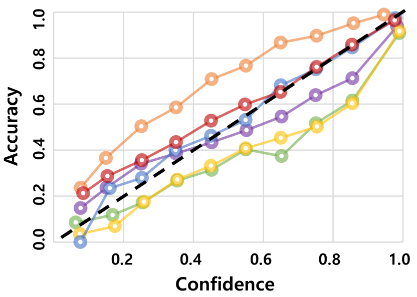
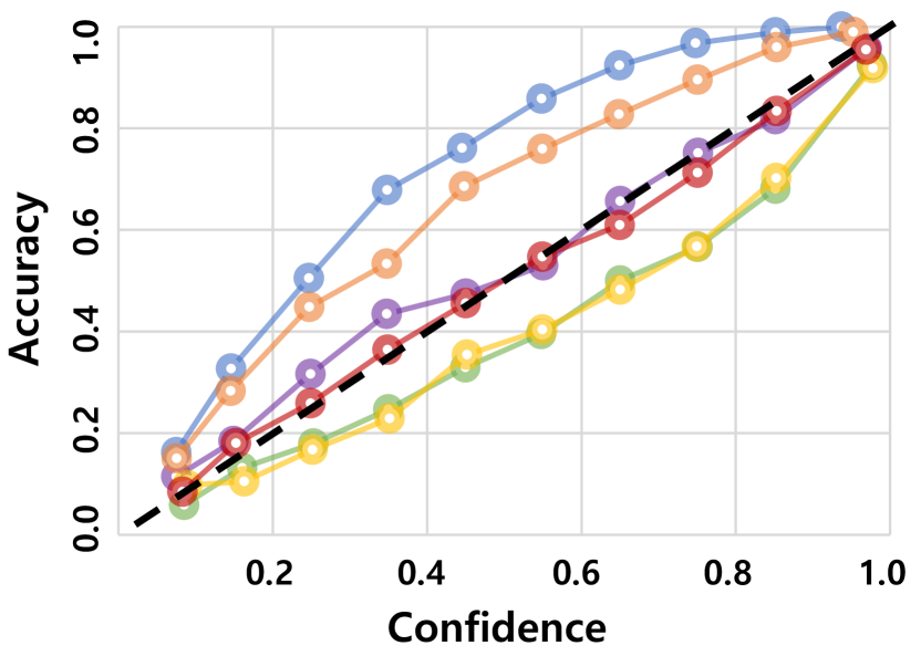
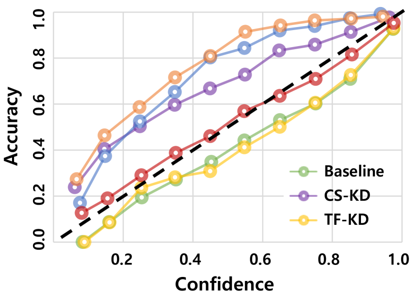
(a) CIFAR-100	(b) Tiny ImageNet	(c) CUB200-2011
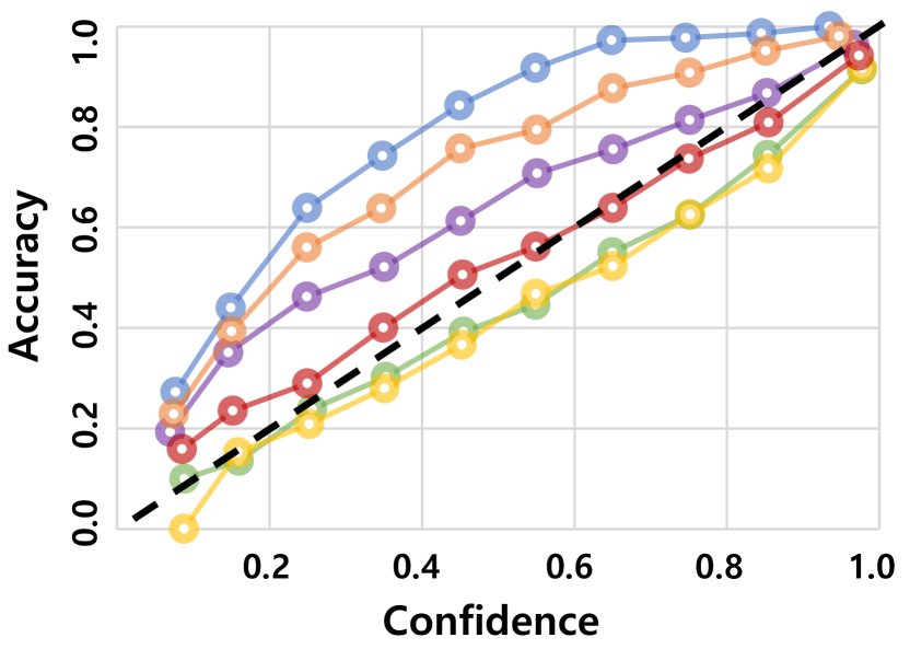
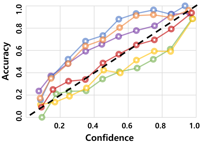
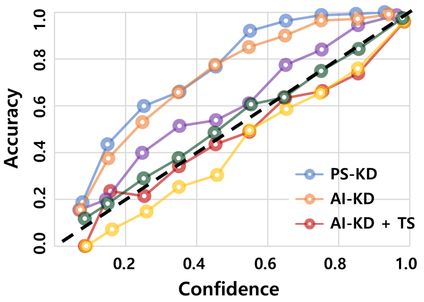
(d) Stanford Dogs	(e) MIT67	(f) FGVC Aircraft

Figure 4: Confidence reliability diagrams based on ResNet-18 with various datasets.

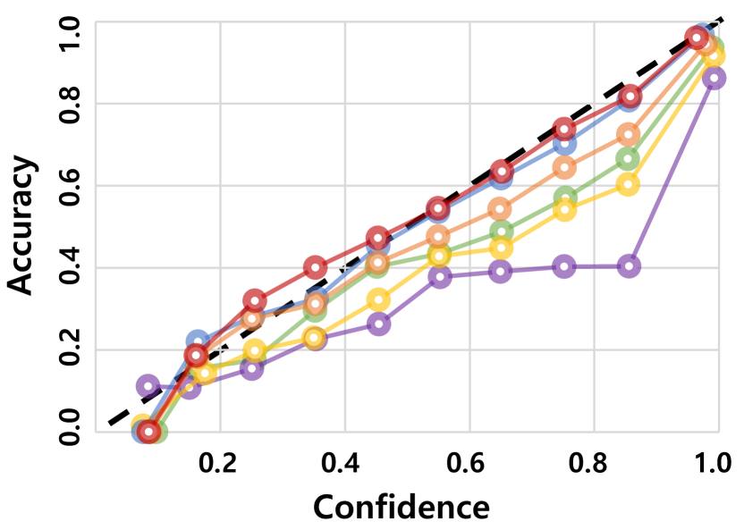
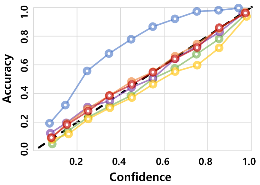
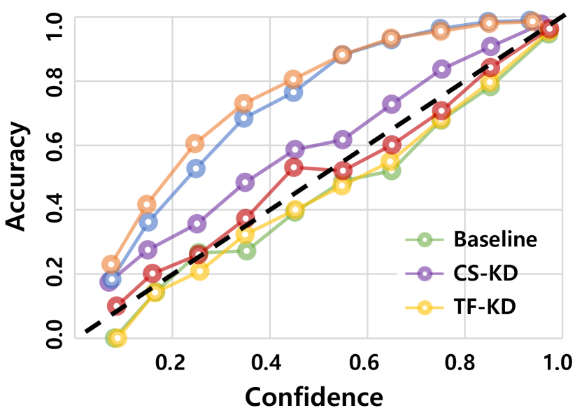
(a) CIFAR-100	(b) Tiny ImageNet	(c) CUB200-2011
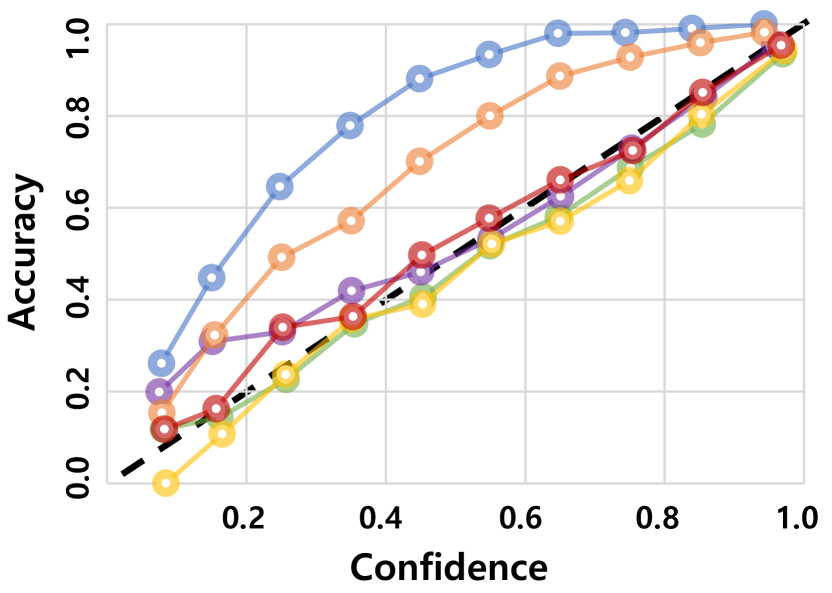
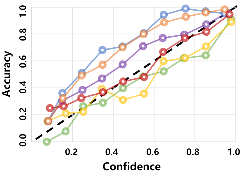
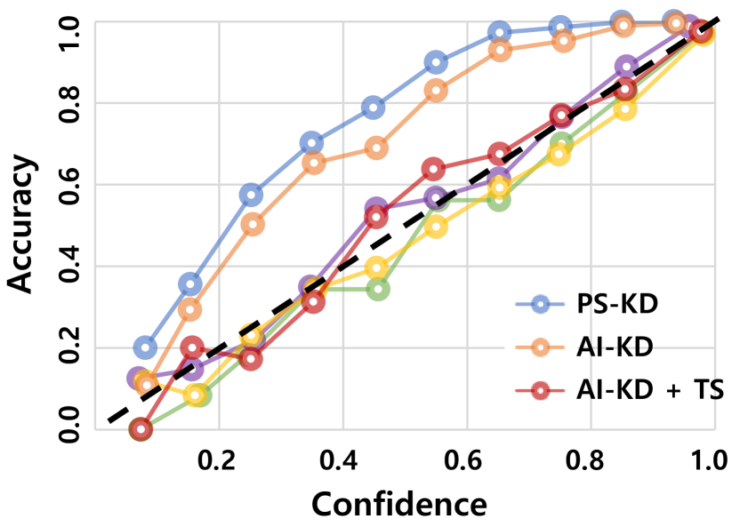
(d) Stanford Dogs	(e) MIT67	(f) FGVC Aircraft

Figure 5: Confidence reliability diagrams based on DenseNet-121 with various datasets.

To further evaluate the our proposed method, Table 3 shows the comparison results in terms of Top-5 error rate and ECE. AI-KD provides the best Top-5 error rate with CIFAR-100, CUB200-2011, and Stanford Dogs datasets on ResNet-18. Also, on DenseNet-121, we confirm that AI-KD record the best Top-5 error with all the fine-grained datasets such as CUB200-2011, Stanford Dogs, MIT67, and FGVC aircraft. Even the results which recorded the second-best performances not the best are competitive and close to the best results by other state-of-the-art methods.

Unlike other metrics, ECE is the metric to measure a model based on calibration error and is calculated as a weighted average over the absolute difference between accuracy and confidence. AI-KD shows tendencies to be over-confidence under all datasets and network models, except for an evaluation with Tiny-ImageNet on DenseNet-121. However, the drawback can alleviate and prevent degradation using the calibration method by temperature scaling [34]. We conduct additional experiments to employ the calibration method and confirm the results. Applying the temperature scaling, AI-KD records well-calibrated results and is alleviated over-confidence, as shown in Table 3 TS rows. For better intuitive analysis, we describe the ECE result using confidence reliability diagrams with the datasets on ResNet-18 and DenseNet-121. The plotted diagonal dot lines in each figure indicate the identity function. The closer each solid line by the considered method to the diagonal dot lines, the method indicates well-calibrated. Figure 4 describes the results on ResNet-18 with all evaluated datasets. The solid orange line indicates confidence in our proposed method and is plotted over the diagonal line with all datasets. Employing temperature scaling to AI-KD, we confirm that the result, the solid red line, is plotted close to the diagonal dot line. We also plot the reliability diagrams of our proposed method on DenseNet-121, as shown in Figure 5 and confirm the effectiveness as same with the results of ResNet-18 network model.

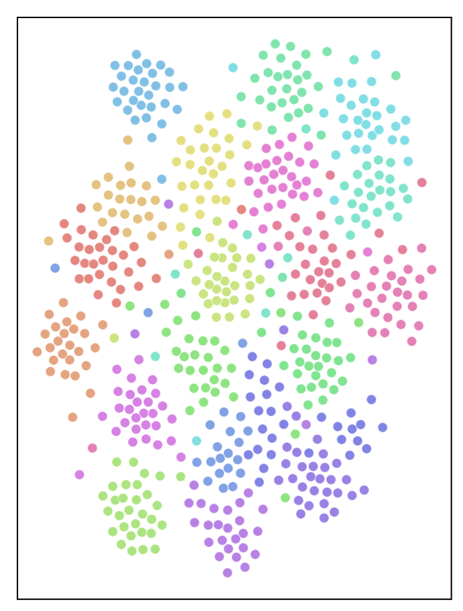
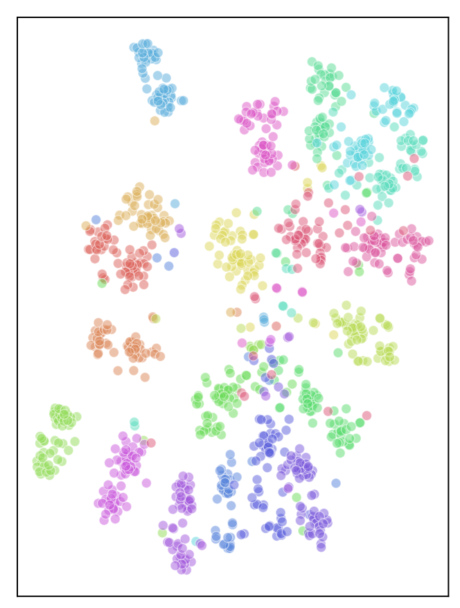
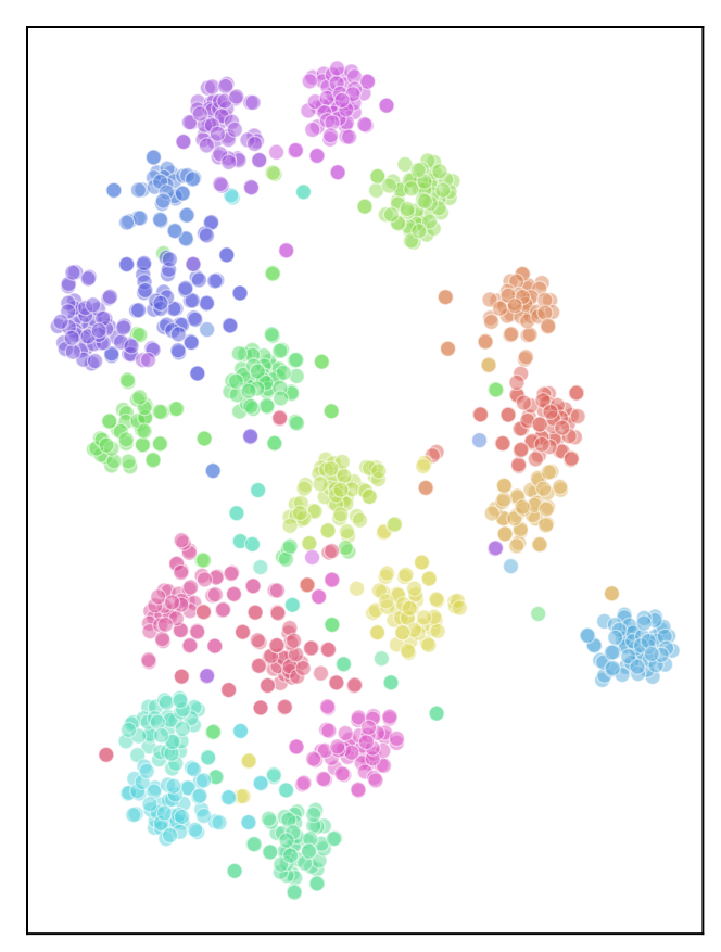
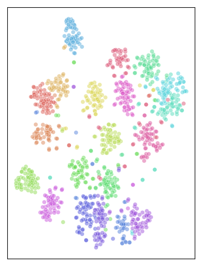
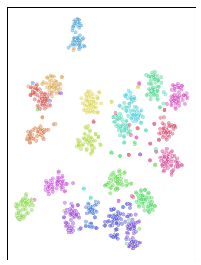
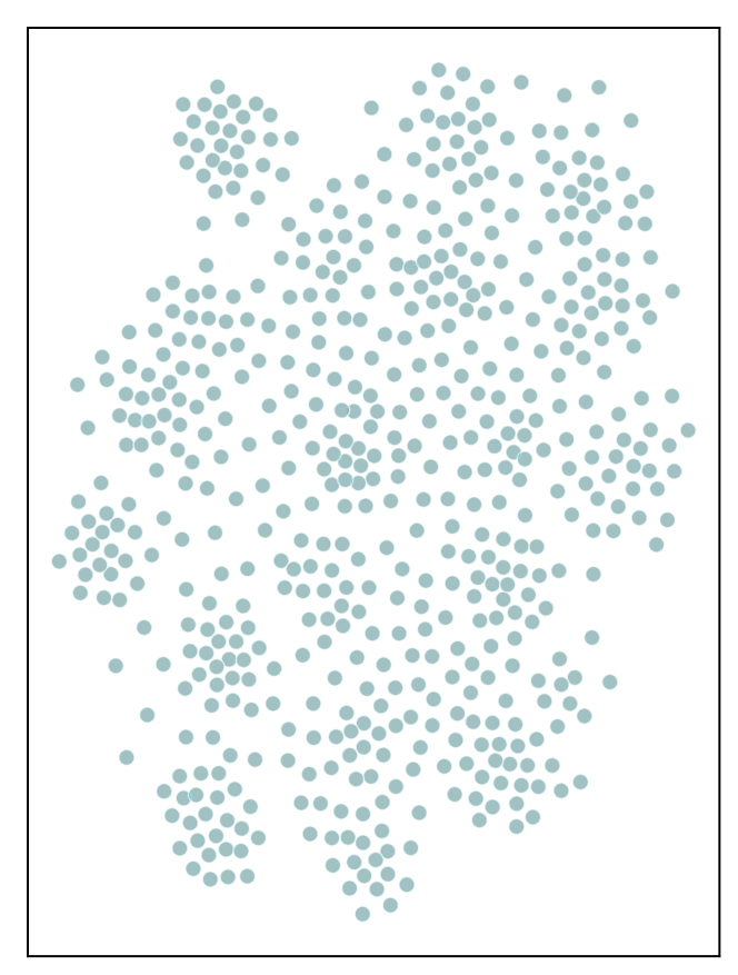
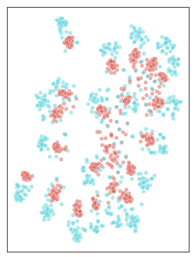
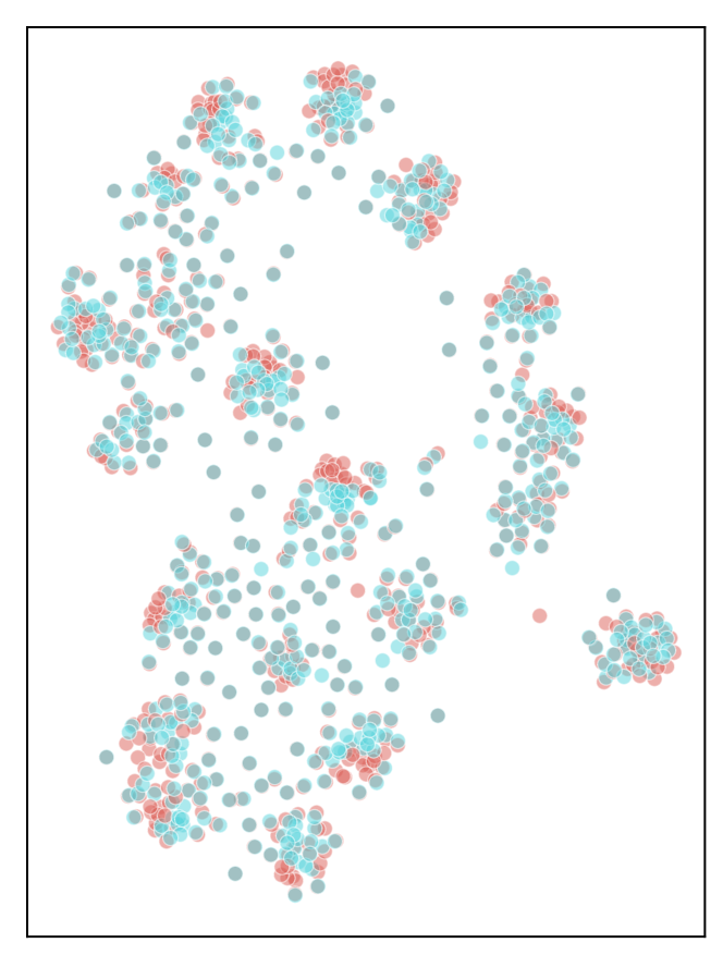
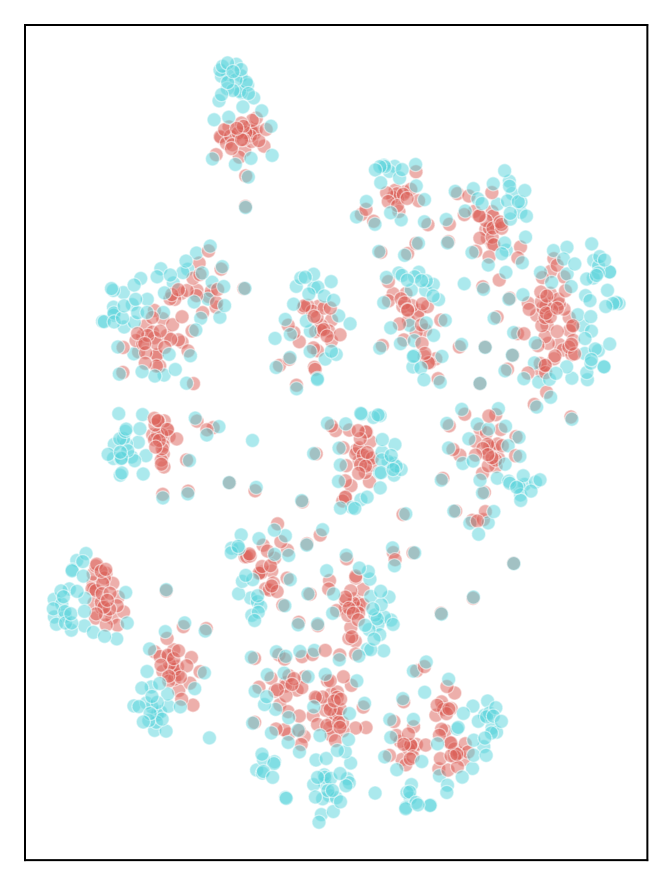
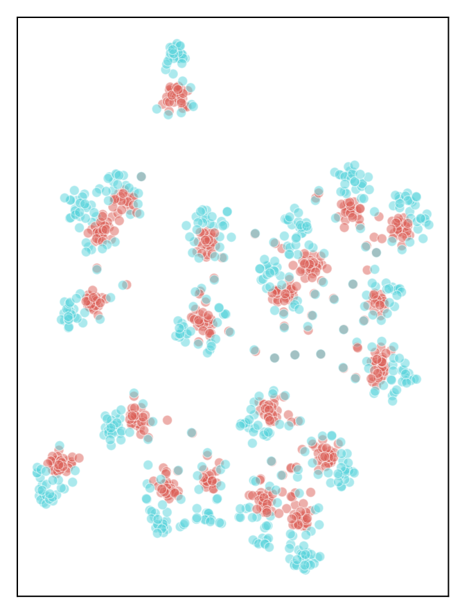
(a) Baseline	(b) CS-KD	(c) TF-KD	(d) PS-KD	(e) AI-KD

Figure 6: t-SNE by arbitrary selected 20 classes on ResNet-18 with CUB200-2011. In the top row, different colors indicate each class. In the bottom row, red and blue dots indicate the extracted features from the student and the superior model, respectively.

We visualize the benefits of our proposed method using t-SNE [35]. Figure 6 shows the t-SNE visualization examples compared to state-of-the-art methods on CUB200-2011 dataset with arbitrary selected 20 classes for better visualization. The top row describes how well-clustered samples are in each class by the methods, and colors indicate different classes. AI-KD tends to have more extensive inter-class variances than other methods, showing outstanding classification performance. The bottom row shows the dependence degree of the student model on the pre-trained model. Blue and red dots indicate features extracted from $S^{Sup}$ and $S_{t}$, respectively. Because CS-KD does not utilize $S^{Sup}$, the pre-trained dots depict far from the student dots. In contrast, the t-SNE image by TF-KD shows that most red dots are overlapped with blue dots so that the student model is directly aligned to the pre-trained model and highly dependent on the pre-trained model. Meanwhile, the visualized result by AI-KD shows that the student features (red dots) place near the pre-trained features (blue dots) or overlapped with blue dots partially. Also, AI-KD tends to concentrate on specific points of each class than blue dots. It represents AI-KD aligns the distribution of the student model to the one of the pre-trained model.

4.4 Ablation studies on AI-KD

In this section, we analyze the effectiveness of our proposed method using various ablation studies and experiments. First, we explore the impact of our proposed losses using an ablation study and then confirm the necessity of the adversarial loss function. And by evaluating variants of the discriminator model, a suitable discriminator architecture is designated to lead to the best classification performance. Also, we experiment to search fitted temperature scaling parameters to better distill knowledge from $S^{Sup}$ and $S_{t-1}$ to $S_{t}$. Lastly, AI-KD has four proposed losses, and we conduct evaluations to find the balancing weights of each loss.

Table 4: Loss ablation study result with ResNet-18 on CIFAR-100. We report the mean and standard deviation over three runs. The best and second-best results are indicated in bold and underlined. Each loss which are $\mathcal{L}_{CE}$, $\mathcal{L}_{G}$, $\mathcal{L}_{P}$, and $\mathcal{L}_{A}$, are indicated the loss of the cross-entropy, guide, previous epoch, and adversarial, respectively.

Model	Method	Top-1 Err ($\%$)	Top-5 Err ($\%$)
ResNet-18	AI-KD	19.87$\pm$0.07	4.81$\pm$0.04
	No Adv	20.34$\pm$0.28	4.86$\pm$0.10
	Only Progressive	21.26$\pm$0.06	5.66$\pm$0.06
	Only Guide	22.17$\pm$0.05	6.21$\pm$0.22
	Baseline	23.97$\pm$0.29	6.80$\pm$0.02

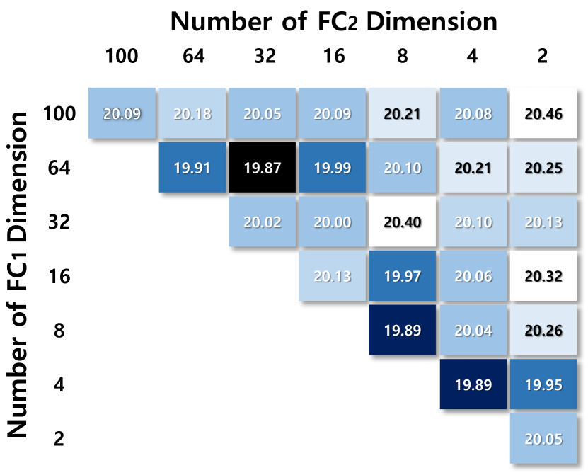
(a) Discriminator layers	(b) Temperature scaling, $\tau_{G}$ and $\tau_{P}$ for KD

Figure 7: Top-1 errors for the number of dimensions in the discriminator, and temperature parameters on ResNet-18 [10] with CIFAR-100 dataset [28].

Efficacy of the proposed losses

AI-KD utilizes two loss functions with different objectives, which are $\mathcal{L}_{D}$ and $\mathcal{L}_{AI}$, as in Equations 6 and  8. $\mathcal{L}_{D}$ penalizes the discriminator to distinguish better the predictive distributions that are the pre-trained and the student models. $\mathcal{L}_{AI}$ supports regularizing $S_{t}$ using distilled information from $S^{Sup}$ and $S_{t-1}$. To verify the benefits of the proposed adversarial and progressive learning scheme, we derive four variants of the proposed method, named ‘No Adv’, ‘Only Progressive’, ‘Only Guide’, and ‘Baseline’. ‘No Adv’ is to train the student model with the pre-trained model without adversarial learning, ‘Only Progressive’ denotes that the student model is trained by the progressive regularization $\mathcal{L}_{P}$ without pre-trained model, ‘Only Guide’ is implemented with the pre-trained model and the guide loss $\mathcal{L}_{G}$, and $\mathcal{L}_{G}$, and ‘Baseline’ refers to the basic student model trained only with the standard cross-entropy, $\mathcal{L}_{CE}$ for $S_{t}$. Table 4 shows the effectiveness of the proposed method compared to its four variants on CIFAR-100 dataset with ResNet-18 in terms of Top-1 error and Top-5 error. The baseline recorded the worst performance and the proposed AI-KD outperformed the four variants in terms of Top-1 and Top-5 errors. As shown in Table 4 on the third and fourth row, we confirm the effectiveness of the progressive regularization and guide loss by the improved performances from the baseline by $+1.80\%$ and $+2.71\%$ in Top-1 error rates, respectively. In addition, ‘No Adv’ provided the second-best result in terms of Top-1 and Top-5 errors. Through employing adversarial learning scheme, $S_{t}$ not only can learn to mimic the predictive probabilities of $S^{Sup}$ but also align the distributions between $S^{Sup}$ and $S_{t}$. In this manner, AI-KD leads outperform the other variants and shows state-of-the-art performance.

Discriminator structure

AI-KD utilizes a discriminator network, and it consists of one activated function and one batch normalization, and two FC layers. Each FC layer is denoted $FC_{1}$ and $FC_{2}$, and then each FC layer has a different dimension to better distinguish the distributions from $S^{Sup}$ or $S_{t}$. In other words, the number of input features of $FC_{1}$ depends on the dataset since the dataset has different classification classes. We conduct experiments to find appropriate parameters of dimension, which are the number of output features of $FC_{1}$ and $FC_{2}$. The results are reported to calculate as the mean value using Top-1 error rates over three runs, as shown in Figure 7(a). The best performance is measured where $FC_{1}$ has the number of output feature at 64 and $FC_{2}$ has the parameter at 32, respectively. From the experiment results, we set the discriminator at FC layer (64)-1D Batch Normalization-LeakyReLU-FC layer (32) and apply to our proposed method, AI-KD.

Distillation temperature

To improve generality and better distill information from each model, the temperature scaling parameter is controlled to generate the soft targets from logits. And then the soft targets contain the informative dark knowledge from each model. AI-KD utilizes two different temperature scaling parameters which are $\tau_{G}$ and $\tau_{P}$. We have evaluated the parameters in the range from one to seven, for the best performance. As shown in Figure 7(b), we set to optimize the parameters for $\mathcal{L}_{G}$ at 3 and for $\mathcal{L}_{P}$ at 1, respectively.

Table 5: Ablation of adversarial loss weight ($\omega$) result on ResNet-18 with CIFAR-100. We report the mean and standard deviation over three runs. The best and second-best results are indicated in bold and underlined, respectively.

Model	$\omega$	Top-1 Err ($\%$)	Top-5 Err ($\%$)
ResNet-18	0.00	20.34$\pm$0.28	4.86$\pm$0.10
	0.01	19.91$\pm$0.17	4.82$\pm$0.14
	0.05	19.97$\pm$0.22	4.85$\pm$0.25
	0.10	19.87$\pm$0.07	4.81$\pm$0.04
	0.25	19.97$\pm$0.09	4.89$\pm$0.09
	0.50	20.17$\pm$0.12	4.90$\pm$0.22
	0.75	20.42$\pm$0.04	5.27$\pm$0.29
	1.00	20.42$\pm$0.04	5.27$\pm$0.29

Table 6: Balanced weight ablation results based with ResNet-18 on CIFAR-100. We report the mean and standard deviation over three runs. The best results are indicated in bold.

Weight				Top-1 Err ($\%$)	Top-5 Err ($\%$)
$\alpha_{CE}$	$\alpha_{G}$	$\alpha_{P}$
0.6	0.1	0.3		19.87$\pm$0.07	4.81$\pm$0.04
0.6	0.2	0.2		21.29$\pm$0.12	5.46$\pm$0.09
0.6	0.3	0.1		22.05$\pm$0.17	5.62$\pm$0.11
0.7	0.1	0.2		20.98$\pm$0.09	5.24$\pm$0.12
0.7	0.2	0.1		21.79$\pm$0.13	5.48$\pm$0.07
0.8	0.1	0.1		21.46$\pm$0.11	5.16$\pm$0.20

Balancing weight parameter of the losses

We experiment the adversarial loss variants, $\omega\in\{0.0,0.01,0.1,0.5,1.0\}$ to set proper weight. As shown in Table 5, the classification performance is not sensitive to $\omega$ ranging from 0.01 to 0.5, though $\omega=0.1$ yields the best performance in the experiment. Also, the loss of AI-KD consists of four losses that are cross-entropy loss, guide loss, progressive loss, and adversarial loss, denoted $\mathcal{L}_{CE}$, $\mathcal{L}_{G}$, $\mathcal{L}_{P}$, and $\mathcal{L}_{D}$, respectively. And the losses have balancing weights, such as $\alpha_{CE}$, $\alpha_{G}$, $\alpha_{P}$, and $\omega$. As we confirmed in the main paper, the weight of adversarial loss, $\omega$ is optimized to 0.1. In this section, we confirm other weights, $\alpha_{CE}$, $\alpha_{G}$, $\alpha_{P}$. Since these parameters are balancing weight, the sum of weight should be 1. We verify the variants as described in Table 6, AI-KD shows the best performance where the weight of $\alpha_{CE}$, $\alpha_{G}$, and $\alpha_{P}$ are 0.6, 0.1, and 0.3, respectively.

Table 7: Compatibility results with data augmentation based on ResNet-18 with CIFAR-100. We report the mean and standard deviation over three runs.

Method	Top-1 Err ($\%$)	Top-5 Err ($\%$)
AI-KD	19.87$\pm$0.07	4.81$\pm$0.04
+ Cutout [36]	19.75$\pm$0.29	4.90$\pm$0.01
+ Mixup [37]	19.29$\pm$0.16	4.70$\pm$0.12
+ CutMix [38]	18.97$\pm$0.25	4.32$\pm$0.10

4.5 Compatibility with data augmentations

Self-KD is one of the regularization methods. And the regularization can be combined with other regularization techniques orthogonally. For this reason, we conducted compatibility experiments with well-known data augmentation techniques, such as Cutout [36], Mixup [37], and CutMix [38]. Cutout removes a randomly selected square region in images. Mixup generates additional data from existing training data by combining samples with an arbitrary mixing rate. CutMix combines Mixup and Cutout methods and generates new samples are generated by replacing patches of random regions cropped from other images. As shown in Table 7, we observe that Top-1 error rate records 19.75$\%$, 19.29$\%$, and 18.97$\%$ when our method is combined with Cutout, Mixup, and CutMix, respectively. And the all results present improved performance than AI-KD without data augmentation techniques. It shows the broad applicability of our method for use with other regularization methods.

5 Conclusion

In this paper, we presented a novel self-knowledge distillation method using adversarial learning to improve the generalization of DNNs. The proposed method, AI-KD, distills deterministic and progressive knowledge from superior model’s and the previous student’s so that the student model learns stable. By applying adversarial learning, the student learns not only to mimic the corresponding network but also to consider aligning the distributions from the superior pre-trained model. Compared to state-of-the-art Self-KD methods, AI-KD presented better image classification performances in terms of Top-1 error, Top-5 Error, and F1 score with network architectures on various datasets. In particular, our proposed method recorded outstanding performances on fine-grained datasets. In addition, the ablation study showed the advantages of the proposed adversarial learning and implicit regularization. Also, we demonstrated the compatibility with data augmentation methods. Regardless, AI-KD still has a limitation which is requiring the pre-trained model. The pre-trained model is essential since it mimics distributions and utilizes adversarial learning. However, the requirement hinders end-to-end learning. For future work, we look forward to proposing a KD method without the pre-trained model, so that developing sustainable DNNs. Furthermore, we plan to extend AI-KD to continual learning and multimodal machine learning.

References

- [1] N. Srivastava, G. Hinton, A. Krizhevsky, I. Sutskever, R. Salakhutdinov, Dropout: a simple way to prevent neural networks from overfitting, The journal of machine learning research (2014) 1929–1958.
- [2] S. Ioffe, C. Szegedy, Batch normalization: Accelerating deep network training by reducing internal covariate shift, in: Proc. ICML, 2015, pp. 448–456.
- [3] C. Szegedy, V. Vanhoucke, S. Ioffe, J. Shlens, Z. Wojna, Rethinking the inception architecture for computer vision, in: Proc. CVPR, 2016, pp. 2818–2826.
- [4] G. Pereyra, G. Tucker, J. Chorowski, Ł. Kaiser, G. Hinton, Regularizing neural networks by penalizing confident output distributions, arXiv preprint arXiv:1701.06548.
- [5] G. Hinton, O. Vinyals, J. Dean, Distilling the knowledge in a neural network, NeurlIPS Workshop on Deep Learning and Representation Learning.
- [6] Y. Jang, H. Lee, S. J. Hwang, J. Shin, Learning what and where to transfer, in: Proc. ICLR, PMLR, 2019, pp. 3030–3039.
- [7] S. I. Mirzadeh, M. Farajtabar, A. Li, N. Levine, A. Matsukawa, H. Ghasemzadeh, Improved knowledge distillation via teacher assistant, in: Proc. AAAI, Vol. 34, 2020, pp. 5191–5198.
- [8] L. Yuan, F. E. Tay, G. Li, T. Wang, J. Feng, Revisiting knowledge distillation via label smoothing regularization, in: Proc. CVPR, 2020, pp. 3903–3911.
- [9] K. Kim, B. Ji, D. Yoon, S. Hwang, Self-knowledge distillation with progressive refinement of targets, in: Proc. ICCV, 2021, pp. 6567–6576.
- [10] K. He, X. Zhang, S. Ren, J. Sun, Deep residual learning for image recognition, in: Proc. CVPR, 2016, pp. 770–778.
- [11] K. He, X. Zhang, S. Ren, J. Sun, Identity mappings in deep residual networks, in: Proc. ECCV, Springer, 2016, pp. 630–645.
- [12] G. Huang, Z. Liu, L. Van Der Maaten, K. Q. Weinberger, Densely connected convolutional networks, in: Proc. CVPR, 2017, pp. 4700–4708.
- [13] L. Zhang, J. Song, A. Gao, J. Chen, C. Bao, K. Ma, Be your own teacher: Improve the performance of convolutional neural networks via self distillation, in: Proc. ICCV, 2019.
- [14] X. Wang, Y. Li, Harmonized dense knowledge distillation training for multi-exit architectures, in: Proc. AAAI, 2021, pp. 10218–10226.
- [15] T.-B. Xu, C.-L. Liu, Data-distortion guided self-distillation for deep neural networks, in: Proc. AAAI, 2019, pp. 5565–5572.
- [16] S. Yun, J. Park, K. Lee, J. Shin, Regularizing class-wise predictions via self-knowledge distillation, in: Proc. CVPR, 2020.
- [17] J. Wang, P. Zhang, Y. Li, Memory-replay knowledge distillation, Sensors 21 (2021) 2792.
- [18] Y. Shen, L. Xu, Y. Yang, Y. Li, Y. Guo, Self-distillation from the last mini-batch for consistency regularization, arXiv preprint arXiv:2203.16172.
- [19] C. Yang, L. Xie, C. Su, A. L. Yuille, Snapshot distillation: Teacher-student optimization in one generation, in: Proc. CVPR, 2019.
- [20] T. Furlanello, Z. Lipton, M. Tschannen, L. Itti, A. Anandkumar, Born again neural networks, in: Proc. ICML, 2018, pp. 1607–1616.
- [21] I. Goodfellow, J. Pouget-Abadie, M. Mirza, B. Xu, D. Warde-Farley, S. Ozair, A. Courville, Y. Bengio, Generative adversarial nets, NeurlIPS 27.
- [22] I. Gulrajani, F. Ahmed, M. Arjovsky, V. Dumoulin, A. C. Courville, Improved training of wasserstein gans, NeurlIPS 30.
- [23] G. Fang, J. Song, C. Shen, X. Wang, D. Chen, M. Song, Data-free adversarial distillation, arXiv preprint arXiv:1912.11006.
- [24] P. Micaelli, A. J. Storkey, Zero-shot knowledge transfer via adversarial belief matching, NeurlIPS 32.
- [25] Y. Choi, J. P. Choi, M. El-Khamy, J. Lee, Data-free network quantization with adversarial knowledge distillation, IEEE/CVF Conference on Computer Vision and Pattern Recognition Workshops (2020) 3047–3057.
- [26] I. Chung, S. Park, J. Kim, N. Kwak, Feature-map-level online adversarial knowledge distillation, in: Proc. ICML, 2020, pp. 2006–2015.
- [27] Q. Xu, Z. Chen, M. Ragab, C. Wang, M. Wu, X. Li, Contrastive adversarial knowledge distillation for deep model compression in time-series regression tasks, Neurocomputing 485 (2022) 242–251.
- [28] A. Krizhevsky, G. Hinton, et al., Learning multiple layers of features from tiny images, Technical report.
- [29] C. Wah, S. Branson, P. Welinder, P. Perona, S. Belongie, The caltech-ucsd birds-200-2011 dataset, Technical report.
- [30] A. Khosla, N. Jayadevaprakash, B. Yao, F.-F. Li, Novel dataset for fine-grained image categorization: Stanford dogs, in: Proc. CVPR Workshop on Fine-Grained Visual Categorization, 2011.
- [31] A. Quattoni, A. Torralba, Recognizing indoor scenes, in: Proc. CVPR, 2009, pp. 413–420.
- [32] S. Maji, E. Rahtu, J. Kannala, M. Blaschko, A. Vedaldi, Fine-grained visual classification of aircraft, arXiv preprint arXiv:1306.5151.
- [33] M. P. Naeini, G. Cooper, M. Hauskrecht, Obtaining well calibrated probabilities using bayesian binning, in: Proc. AAAI, 2015.
- [34] C. Guo, G. Pleiss, Y. Sun, K. Q. Weinberger, On calibration of modern neural networks, in: Proc. ICML, 2017.
- [35] L. van der Maaten, G. Hinton, Visualizing data using t-sne, Journal of Machine Learning Research 9 (86) (2008) 2579–2605.
- [36] T. DeVries, G. W. Taylor, Improved regularization of convolutional neural networks with cutout, arXiv preprint arXiv:1708.04552.
- [37] H. Zhang, M. Cisse, Y. N. Dauphin, D. Lopez-Paz, mixup: Beyond empirical risk minimization, in: Proc. ICLR, 2018.
- [38] S. Yun, D. Han, S. J. Oh, S. Chun, J. Choe, Y. Yoo, Cutmix: Regularization strategy to train strong classifiers with localizable features, in: Proc. ICCV, 2019, pp. 6023–6032.