Deep Reinforcement Learning Guided Improvement Heuristic for Job Shop Scheduling

Abstract

Recent studies in using deep reinforcement learning (DRL) to solve Job-shop scheduling problems (JSSP) focus on construction heuristics. However, their performance is still far from optimality, mainly because the underlying graph representation scheme is unsuitable for modelling partial solutions at each construction step. This paper proposes a novel DRL-guided improvement heuristic for solving JSSP, where graph representation is employed to encode complete solutions. We design a Graph-Neural-Network-based representation scheme, consisting of two modules to effectively capture the information of dynamic topology and different types of nodes in graphs encountered during the improvement process. To speed up solution evaluation during improvement, we present a novel message-passing mechanism that can evaluate multiple solutions simultaneously. We prove that the computational complexity of our method scales linearly with problem size. Experiments on classic benchmarks show that the improvement policy learned by our method outperforms state-of-the-art DRL-based methods by a large margin.

1 Introduction

Recently, there has been a growing trend towards applying deep (reinforcement) learning (DRL) to solve combinatorial optimization problems (Bengio et al., 2020). Unlike routing problems that are vastly studied (Kool et al., 2018; Xin et al., 2021a; Hottung et al., 2022; Kwon et al., 2020; Ma et al., 2023; Zhou et al., 2023; Xin et al., 2021b), the Job-shop scheduling problem (JSSP), a well-known problem in operations research ubiquitous in many industries such as manufacturing and transportation, received relatively less attention.

Compared to routing problems, the performance of existing learning-based solvers for scheduling problems is still quite far from optimality due to the lack of an effective learning framework and neural representation scheme. For JSSP, most existing learning-based approaches follow a dispatching procedure that constructs schedules by extending partial solutions to complete ones. To represent the constructive states, i.e. partial solutions, they usually employ disjunctive graph (Zhang et al., 2020; Park et al., 2021b) or augment the graph with artificial machine nodes (Park et al., 2021a). Then, a Graph Neural Network (GNN) based agent learns a latent embedding of the graphs and outputs construction actions. However, such representation may not be suitable for learning construction heuristics. Specifically, while the agent requires proper work-in-progress information of the partial solution during each construction step (e.g. the current machine load and job status), it is hard to incorporate them into a disjunctive graph, given that the topological relationships could be more naturally modelled among operations (Balas, 1969). Consequently, with the important components being ignored due to the solution incompleteness, such as the disjunctive arcs among undispatched operations (Zhang et al., 2020) and the orientations of disjunctive arcs among operations within a machine clique (Park et al., 2021b), the partial solution representation by disjunctive graphs in current works may suffer from severe biases. Therefore, one question that comes to mind is: Can we transform the learning-to-schedule problem into a learning-to-search-graph-structures problem to circumvent the issue of partial solution representation and significantly improve performance?

Compared to construction ones, improvement heuristics perform iterative search in the neighbourhood for better solutions. For JSSP, a neighbour is a complete solution, which is naturally represented as a disjunctive graph with all the necessary information. Since searching over the space of disjunctive graphs is more effective and efficient, it motivates a series of breakthroughs in traditional heuristic methods (Nowicki & Smutnicki, 2005; Zhang et al., 2007). In traditional JSSP improvement heuristics, local moves in the neighbourhood are guided by hand-crafted rules, e.g. picking the one with the largest improvement. This inevitably brings two major limitations. Firstly, at each improvement step, solutions in the whole neighbourhood need to be evaluated, which is computationally heavy, especially for large-scale problems. Secondly, the hand-crafted rules are often short-sighted and may not take future effects into account, therefore could limit the improvement performance.

In this paper, we propose a novel DRL-based improvement heuristic for JSSP that addresses the above limitations, based on a simple yet effective improvement framework. The local moves are generated by a deep policy network, which circumvents the need to evaluate the entire neighbourhood. More importantly, through reinforcement learning, the agent is able to automatically learn search policies that are longer-sighted, leading to superior performance. While a similar paradigm has been explored for routing problems (Chen & Tian, 2019; Lu et al., 2019; Wu et al., 2021), it is rarely touched in the scheduling domain. Based on the properties of JSSP, we propose a novel GNN-based representation scheme to capture the complex dynamics of disjunctive graphs in the improvement process, which is equipped with two embedding modules. One module is responsible for extracting topological information of disjunctive graph, while the other extracts embeddings by incorporating the heterogeneity of nodes’ neighbours in the graph. The resulting policy has linear computational complexity with respect to the number of jobs and machines when embedding disjunctive graphs. To further speed up solution evaluation, especially for batch processing, we design a novel message-passing mechanism that can evaluate multiple solutions simultaneously.

We verify our method on seven classic benchmarks. Extensive results show that our method generally outperforms state-of-the-art DRL-based methods by a large margin while maintaining a low computational cost. On large-scale instances, our method even outperforms Or-tools CP-SAT, a highly efficient constraint programming solver. Our aim is to showcase the effectiveness of Deep Reinforcement Learning (DRL) in learning superior search control policies compared to traditional methods. Our computationally efficient DRL-based heuristic narrows the performance gap with existing techniques and outperforms a tabu search algorithm in experiments. Furthermore, our method can potentially be combined with more complicated improvement frameworks, however it is out of the scope of this paper and will be investigated in the future.

2 Related Work

Most existing DRL-based methods for JSSP focus on learning dispatching rules, or construction heuristics. Among them, L2D (Zhang et al., 2020) encodes partial solutions as disjunctive graphs and a GNN-based agent is trained via DRL to dispatch jobs to machines to construct tight schedules. Despite the superiority to traditional dispatching rules, its graph representation can only capture relations among dispatched operations, resulting in relatively large optimality gaps. A similar approach is proposed in (Park et al., 2021b). By incorporating heterogeneity of neighbours (e.g. predecessor or successor) in disjunctive graphs, a GNN model extracts separate embeddings and then aggregates them accordingly. While delivering better solutions than L2D, this method suffers from static graph representation, as the operations in each machine clique are always fully connected. Therefore, it fails to capture structural differences among solutions, which we notice to be critical. For example, given a JSSP instance, the processing order of jobs on each machine could be distinct for each solution, which cannot be reflected correctly in the respective representation scheme. ScheduleNet (Park et al., 2021a) introduces artificial machine nodes and edges in the disjunctive graph to encode machine-job relations. The new graph enriches the expressiveness but is still static. A Markov decision process formulation with a matrix state representation is proposed in (Tassel et al., 2021). Though the performance is ameliorated, it is an online method that learns for each instance separately, hence requiring much longer solving time. Moreover, unlike the aforementioned graph-based ones, the matrix representation in this method is not size-agnostic, which cannot be generalised across different problem sizes. RASCL (Iklassov et al., 2022) learns generalized dispatching rules for solving JSSP, where the solving process is modelled as MDPs. Tassel et al. (2023a) propose to leverage existing Constraint Programming (CP) solvers to train a DRL-agent learning a Priority Dispatching Rule (PDR) that generalizes well to large instances. Despite substantial improvement, the performance of these works is still far from optimality compared with our method. Other learning-based construction heuristics for solving variants of JSSP include FFSP (Choo et al., 2022; Kwon et al., 2021) and scheduling problems in semiconductor manufacturing (Tassel et al., 2023b). However, these methods are incompatible with JSSP due to their underlying assumption of independent machine sets for each processing stage, which contradicts the shared machine configuration inherent in JSSP.

A work similar to ours is MGRO (Ni et al., 2021), which learns a policy to aid Iterated Greedy (IG), an improvement heuristic, to solve the hybrid flow shop scheduling problem. Our method differs from it in two aspects. Firstly, unlike MGRO which learns to pick local operators from a pool of manually designed ones, our policy does not require such manual work and directly outputs local moves. Secondly, MGRO encodes the current solution as multiple independent subgraphs, which is not applicable to JSSP since it cannot model precedence constraints.

3 Preliminaries

Job-shop Scheduling. A JSSP instance of size $|\mathcal{J}|\times|\mathcal{M}|$ consists of $|\mathcal{J}|$ jobs and $|\mathcal{M}|$ machines. Each job $j\in\mathcal{J}$ is required to be processed by each machine $m\in\mathcal{M}$ in a predefined order $O^{m_{j1}}_{j1}\rightarrow\cdots\rightarrow O^{m_{ji}}_{ji}\rightarrow\cdots\rightarrow O^{m_{j|\mathcal{M}|}}_{j{|\mathcal{M}|}}$ with $O^{m_{ji}}_{ji}$ denoting the $i$th operation of job $j$, which should be processed by the machine $m_{ji}$ with processing time $p_{ji}\in\mathbb{N}$. Let $\mathcal{O}_{j}$ be the collections of all operations for job $j$. Only can the operation $O^{m_{ji}}_{ji}$ be processed when all its precedent operations $\{O^{m_{jz}}_{jz}|z<i\}\subset\mathcal{O}_{j}$ are processed, which is the so-called precedence constraint. The objective is to find a schedule $\eta:\{O^{m_{ji}}_{ji}|\forall j,i\}\rightarrow\mathbb{N}$, i.e., the starting time for each operation, such that the makespan $C_{\max}=\max(\eta(O^{m_{ji}}_{ji})+p_{ji})$ is minimum without violating the precedence constraints. To enhance succinctness, the notation $m_{ji}$ indicating the machine allocation for operation $O_{ji}$ will be disregarded as machine assignments for operations remain constant throughout any given JSSP instance. This notation will be reinstated only if its specification is critical.

Disjunctive Graph. The disjunctive graph (Balas, 1969) is a directed graph $G=(\mathcal{O},\mathcal{C}\cup\mathcal{D})$, where $\mathcal{O}=\{O_{ji}|\forall j,i\}\cup\{O_{S},O_{T}\}$ is the set of all operations, with $O_{S}$ and $O_{T}$ being the dummy ones denoting the beginning and end of processing. $\mathcal{C}$ consists of directed arcs (conjunctions) representing the precedence constraints connecting every two consecutive operations of the same job. Undirected arcs (disjunctions) in set $\mathcal{D}$ connect operations requiring the same machine, forming a clique for each machine. Each arc is labelled with a weight, which is the processing time of the operation that the arc points from (two opposite-directed arcs can represent a disjunctive arc). Consequently, finding a solution $s$ to a JSSP instance is equivalent to fixing the direction of each disjunction, such that the resulting graph $G(s)$ is a DAG (Balas, 1969). The longest path from $O_{S}$ to $O_{T}$ in a solution is called the critical path (CP), whose length is the makespan of the solution. An example of disjunctive graph for a JSSP instance and its solution are depicted in Figure 1.

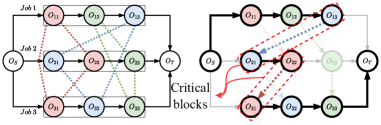
Figure 1: Disjunctive graph representation. Left: a $3\times 3$ JSSP instance. Black arrows are conjunctions. Dotted lines of different colors are disjunctions, grouping operations on each machine into machine cliques. Right: a complete solution, where a critical path and a critical block are highlighted. Arc weights are omitted for clarity.

The $N_{5}$ neighbourhood Structure. Various neighbourhood structures have been proposed for JSSP (Zhang et al., 2007). Here we employ the well-known $N_{5}$ designed based on the concept of critical block (CB), i.e. a group of consecutive operations processed by the same machine on the critical path (refer to Figure 1 for an example). Given a solution $s$, $N_{5}$ constructs the neighbourhood $N_{5}(s)$ as follows. First, it finds the critical path CP(s) of $G(s)$ (randomly selects one if more than one exist). Then for each $CB_{m}=O^{m_{1}}_{1}\rightarrow O^{m_{2}}_{2}\rightarrow\cdots\rightarrow O^{m_{l}}_{l}\rightarrow\cdots\rightarrow O^{m_{L-1}}_{L-1}\rightarrow O^{m_{L}}_{L}$ with $m_{l}$ and $1\leq l\leq L$ denoting the processing machine and the index of operation $O{l}$ along the critical path CP(s), at most two neighbours are obtained by swapping the first $(O^{m_{1}}_{1},O^{m_{2}}_{2})$ or last pair $(O^{m_{L-1}}_{L-1},O^{m_{L}}_{L})$ of operations. Only one neighbour exists if a CB has only two operations. For the first and last CB, only the last and first operation pair are swapped. Consequently, the neighbourhood size $|N_{5}(s)|$ is at most $2N(s)-2$ with $N(s)$ being the number of CBs in $G(s)$.

4 Methodology

The overall framework of our improvement method is shown in Figure 2(a). The initial solution is generated by basic dispatching rules. During the improvement process, solutions are proxied by their graphical counterpart, i.e. disjunctive graphs. Different from traditional improvement heuristics which need to evaluate all neighbours at each step, our method directly outputs an operation pair, which is used to update the current solution according to $N_{5}$. The process terminates if certain condition is met. Here we set it as reaching a searching horizon of $T$ steps.

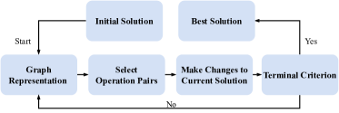
(a) The overall framework of our method.

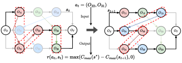
(b) State transition example.

Figure 2: Our local search framework and an example of state transition. In Figure (b), the state $s_{t}$ is transited to $s_{t+1}$ by swapping operation $O_{22}$ and $O_{31}$. A new critical path with its two critical blocks is generated and highlighted in $s_{t+1}$.

Below we present our DRL-based method for learning the pair picking policy. We first formulate the learning task as a Markov decision process (MDP). Then we show how to parameterize the policy based on GNN, and design a customized REINFORCE (Williams, 1992) algorithm to train the policy network. Finally, we design a message-passing mechanism to quickly calculate the schedule, which significantly improves efficiency especially for batch training. Note that, the proposed policy possesses linear computational complexity w.r.t. the number of jobs $|\mathcal{J}|$ and machines $|\mathcal{M}|$.

4.1 The searching procedure as an MDP

States. A state $s_{t}\in\mathcal{S}$ is the complete solution at step $t$, with $s_{0}$ being the initial one. Each state is represented as its disjunctive graph. Features of each node $O_{ji}$ is collected in a vector $\mathbf{x}_{ji}=(p_{ji},est_{ji},lst_{ji})\in\mathbb{R}^{3}$, where $est_{ji}$ and $lst_{ji}$ are the earliest and latest starting time of $O_{ji}$, respectively. For a complete solution, $est(O_{ji})$ is the actual start time of $O_{ji}$ in the schedule. If $O_{ji}$ is located on a critical path, then $est_{ji}=lst_{ji}$ (Jungnickel & Jungnickel, 2005). This should be able to help the agent distinguish whether a node is on the critical path.

Actions. Since we aim at selecting a solution within the neighbourhood, an action $a_{t}$ is one of the operation pairs $(O_{ji},O_{kl})$ in the set of all candidate pairs defined by $N_{5}$. Note that the action space $A_{t}$ is dynamic w.r.t each state.

Transition. The next state $s_{t+1}$ is derived deterministically from $s_{t}$ by swapping the two operations of action $a_{t}=(O_{ji},O_{kl})$ in the graph. An example is illustrated in Figure 2(b), where features $est$ and $lst$ are recalculated for each node in $s_{t+1}$. If there is no feasible action $a_{t}$ for some $t$, e.g. there is only one critical block in $s_{t}$, then the episode enters an absorbing state and stays within it. We present a example in Appendix LABEL:state_transition to facilitate better understanding the state transition mechanism.

Rewards. Our ultimate goal is to improve the initial solution as much as possible. To this end, we design the reward function as follows:

$$r(s_{t},a_{t})=\max\left(C_{max}(s^{*}_{t})-C_{max}(s_{t+1}),0\right),$$ (1)

where $s^{*}_{t}$ is the best solution found until step $t$ (the incumbent), which is updated only if $s_{t+1}$ is better, i.e. $C_{max}(s_{t+1})<C_{max}(s^{*}_{t})$. Initially, $s^{*}_{0}=s_{0}$. The cumulative reward until $t$ is $R_{t}=\sum_{t^{\prime}=0}^{t}r(s_{t^{\prime}},a_{t^{\prime}})=C_{max}(s_{0})-C_{max}(s^{*}_{t})$, which is exactly the improvement against initial solution $s_{0}$. When the episode enters the absorbing state, by definition, the reward is always 0 since there is no possibility of improving the incumbent from then on.

Policy. For state $s_{t}$, a stochastic policy $\pi(a_{t}|s_{t})$ outputs a distribution over the actions in $A_{t}$. If the episode enters the absorbing state, the policy will output a dummy action which has no effect.

4.2 Policy module

We parameterize the stochastic policy $\pi_{\theta}(a_{t}|s_{t})$ as a GNN-based architecture with parameter set $\theta$. A GNN maps the graph to a continuous vector space. The embeddings of nodes could be deemed as feature vectors containing sufficient information to be readily used for various downstream tasks, such as selecting operation pairs for local moves in our case. Moreover, a GNN-based policy is able to generalize to instances of various sizes that are unseen during training, due to its size-agnostic property. The architecture of our policy network is shown in Figure 3.

4.2.1 Graph Embedding

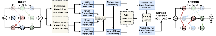
Figure 3: The architecture of our policy network.

For the disjunctive graph, we define a node $U$ as a neighbour of node $V$ if an arc points from $U$ to $V$. Therefore, the dummy operation $O_{S}$ has no neighbours (since there are no nodes pointing to it), and $O_{T}$ has $|\mathcal{J}|$ neighbours (since every job’s last operation is pointing to it). There are two notable characteristics of this graph. First, the topology is dynamically changing due to the MDP state transitions. Such topological difference provides rich information for distinguishing two solutions from the structural perspective. Second, most operations in the graph have two different types of neighbours, i.e. its job predecessor and machine predecessor. These two types of neighbours hold respective semantics. The former is closely related to the precedence constraints, while the latter reflects the processing sequence of jobs on each machine. Based on this observation, we propose a novel GNN with two independent modules to embed disjunctive graphs effectively. We will experimentally prove by an ablation study (section 5.6) that the combination of the two modules are indeed more effective.

Topological Embedding Module. For two different solutions, there must exist a machine on which jobs are processed in different orders, i.e. the disjunctive graphs are topologically different. The first module, which we call topological embedding module (TPM), is expected to capture such structural differences, so as to help the policy network distinguish different states. To this end, we exploit Graph Isomorphism Network (GIN) (Xu et al., 2019), a well-known GNN variant with strong discriminative power for non-isomorphic graphs as the basis of TPM. Given a disjunctive graph $G$, TPM performs $K$ iterations of updates to compute a $p$-dimensional embeddings for each node $V\in\mathcal{O}$, and the update at iteration $k$ is expressed as follows:

$$\mu_{V}^{k}=\text{MLP}_{T}^{k}((1+\epsilon^{k})\mu_{V}^{k-1}+\sum_{U\in\mathcal{N}(V)}\mu_{U}^{k-1}),$$ (2)

where $\mu_{V}^{k}$ is the topological embedding of node $V$ at iteration $k$ and $\mu_{V}^{0}=\mathbf{x}_{ji}$ is its raw features, $\text{MLP}_{T}^{k}$ is a Multi-Layer Perceptron (MLP) for iteration $k$, $\epsilon^{k}$ is an arbitrary number that can be learned, and $\mathcal{N}(V)$ is the neighbourhood of $V$ in $G$. For each $k$, we attain a graph-level embedding $\mu^{k}_{G}\in\mathbb{R}^{p}$ by an average pooling function $L$ with embeddings of all nodes as input as follows:

$$\mu^{k}_{G}=L(\{\mu_{V}^{k}:V\in\mathcal{O}\})=\frac{1}{|\mathcal{O}|}\sum_{V\in\mathcal{O}}\mu_{V}^{k}.$$ (3)

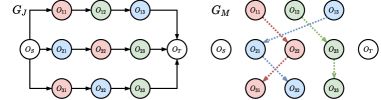
Figure 4: Example of $G_{J}$ and $G_{M}$.

Finally, the topological embeddings of each node and the disjunctive graph after the $K$ iterations are $\{\mu_{V}=\sum_{k}\mu^{k}_{V}:\forall V\in\mathcal{O}\}$ and $\mu_{G}=\sum_{k}\mu^{k}_{G}$, respectively. For representation learning with GIN, layers of different depths learn different structural information (Xu et al., 2019). The representations acquired by the shallow layers sometimes generalize better, while the deeper layers are more oriented for the target task. To consider all the discrepant structural information of the disjunctive graph and align the hidden dimension, we sum the embeddings from all layers.

Context-aware Embedding Module. Now we present the second module to capture information from the two types of neighbouring nodes, which we call context-aware embedding module (CAM). Specifically, we separate a disjunctive graph $G$ into two subgraphs $G_{J}$ and $G_{M}$, i.e. contexts, as shown in Figure 4. Both subgraphs contain all nodes of $G$, but have different sets of edges to reflect respective information. $G_{J}$ contains only conjunctive arcs which represent precedence constraints, while $G_{M}$ contains only (directed) disjunctive arcs to represent the job processing order on each machine. Note that the two dummy nodes $O_{S}$ and $O_{T}$ are isolated in $G_{M}$, since they are not involved in any machine.

Similar to TPM, CAM also updates the embeddings for $K$ iterations by explicitly considering the two contexts during message passing and aggregation. Particularly, the update of node embeddings at CAM iteration $k$ is given as follows:

$$\nu_{V}^{J,k}=\text{GAT}_{J}^{k}\left(\nu_{V}^{k-1},\{\nu_{U}^{k-1}|U\!\in\!\mathcal{N}_{J}(V)\}\right),$$ (4)

$$\nu_{V}^{M,k}=\text{GAT}_{M}^{k}\left(\nu_{V}^{k-1},\{\nu_{U}^{k-1}|U\!\in\!\mathcal{N}_{M}(V)\}\right),$$ (5)

$$\nu_{V}^{k}=\frac{1}{2}\left(\nu_{V}^{J,k}+\nu_{V}^{M,k}\right),$$ (6)

where $\text{GAT}^{k}_{J}$ and $\text{GAT}^{k}_{M}$ are two graph attention layers (Veličković et al., 2018) with $n_{h}$ attention heads, $\nu_{V}^{k}\in\mathbb{R}^{p}$ is the context-aware embedding for $V$ at layer $k$, $\nu_{V}^{J,k}\in\mathbb{R}^{p}$ and $\nu_{V}^{M,k}\in\mathbb{R}^{p}$ are $V$’s embedding for precedence constraints and job processing sequence, and $\mathcal{N}_{J}(V)$ and $\mathcal{N}_{M}(V)$ are $V$’s neighbourhood in $G_{J}$ and $G_{M}$, respectively. For the first iteration, we initialize $\nu_{V}^{0}=\mathbf{x}_{ji},\forall V\!\in\!\mathcal{O}$. Finally, we compute the graph-level context-aware embedding $\nu_{G}$ using average pooling as follows:

$$\nu_{G}=\frac{1}{|\mathcal{O}|}\sum_{V\in\mathcal{O}}\nu_{V}^{K}.$$ (7)

To generate a global representation for the whole graph, we merge the topological and context-aware embeddings by concatenating them and yield:

$$\{h_{V}=(\mu^{K}_{V}:\nu_{V}^{K})|\forall V\in\mathcal{O}\},h_{G}=(\mu_{G}:\nu_{G}).$$ (8)

Remark. We choose GIN as the building block for TPM mainly because it is one of the strongest GNN architectures with proven power to discriminate graphs from a topological point of view. It may benefit identifying topological discrepancies between solutions. As for GAT, it is an equivalent counterpart of Transformers (Vaswani et al., 2017) for graphs, which is a dominant architecture for learning representations from element attributes. Therefore we adopt GAT as the building block of our CAM module to extract node embeddings for the heterogeneous contexts.

4.2.2 Action Selection

Given the node embeddings $\{h_{V}\}$ and graph embedding $h_{G}$, we compute the “score” of selecting each operation pair as follows. First, we concatenate $h_{G}$ to each $h_{V}$, and feed it into a network $\text{MLP}_{A}$, to obtain a latent vector denoted as $h^{\prime}_{V}$ with dimension $q$, which is collected as a matrix $h^{\prime}$ with dimension $|\mathcal{O}|\times q$. Then we multiply $h^{\prime}$ with its transpose $h^{{}^{\prime}\mathsf{T}}$ to get a matrix $SC$ with dimension $|\mathcal{O}|\times|\mathcal{O}|$ as the score of picking the corresponding operation pair. Next, for all pairs that are not included in the current action space, we mask them by setting their scores to $-\infty$. Finally, we flatten the score matrix and apply a softmax function to obtain the probability of selecting each feasible action.

We present the theoretical computational complexity of the proposed policy network. Specifically, for a JSSP instance of size $|\mathcal{J}|\times|\mathcal{M}|$, we can show that:

Theorem 4.1.

The proposed policy network has linear time complexity w.r.t both $|\mathcal{J}|$ and $|\mathcal{M}|$.

The detailed proof is presented in Appendix LABEL:complexity. In the experiments, we will also provide empirical analysis and comparison with other baselines.

4.3 The n-step REINFORCE Algorithm

We propose an n-step REINFORCE algorithm for training the policy network. The motivation, benefits, and details of this algorithm are presented in Appendix A.

4.4 Message-passing for Calculating Schedule

The improvement process requires evaluating the quality of neighbouring solutions by calculating their schedules. In traditional scheduling methods, this is usually done by using the critical path method (CPM) (Jungnickel & Jungnickel, 2005), which calculates the start time for each node recursively. However, it can only process a single graph and cannot make full use of the parallel computing power of GPU. Therefore, traditional CPM is time-costly in processing a batch of instances. To alleviate this issue, we propose an equivalent variant of this algorithm using a message-passing mechanism motivated by the computation of GNN, which enables batch processing and is compatible with GPU.

Our message-passing mechanism works as follows. Given a directed disjunctive graph $G$ representing a solution $s$, we maintain a message $ms_{V}=(d_{V},c_{V})$ for each node $V\in\mathcal{O}$, with initial values $d_{V}=0$ and $c_{V}=1$, except $c_{V}=0$ for $V=O_{S}$. Let $mp_{max}(\cdot)$ denote a message-passing operator with max-pooling as the neighbourhood aggregation function, based on which we perform a series of message updates. During each of them, for $V\in\mathcal{O}$, we update its message by $d_{V}=mp_{max}(\{p_{U}+(1-c_{U})\cdot d_{U}|\forall U\!\in\!\mathcal{N}(V)\})$ and $c_{V}=mp_{max}(\{c_{U}|\forall U\!\in\!\mathcal{N}(V){\color[rgb]{0,0,0}\}})$ with $p_{V}$ and $\mathcal{N}(V)$ being the processing time and the neighbourhood of $V$, respectively. Let $H$ be the number of nodes on the path from $O_{S}$ to $O_{T}$ containing the most nodes. Then we can show that:

Theorem 4.2.

After at most $H$ times of message passing, $d_{V}=est_{V},\forall V\in\mathcal{O}$, and $d_{T}=C_{\text{max}}(s)$.

The proof is presented in Appendix LABEL:proof. This proposition indicates that our message-passing evaluator is equivalent to CPM. It is easy to prove that this proposition also holds for a batch of graphs. Thus the practical run time for calculating the schedule using our evaluator is significantly reduced due to computation in parallel across the batch. We empirically verify the effectiveness by comparing it with CPM (Appendix LABEL:sec:exp-mp).

Similarly, $lst_{V}$ can be calculated by a backward version of our message-passing evaluator where the message is passed from node $O_{T}$ to $O_{S}$ in a graph $\overline{G}$ with all edges reversed. Each node $V$ maintains a message $\overline{ms}_{V}=(\bar{d}_{V},\bar{c}_{V})$. The initial values are $\bar{d}_{V}\!=\!-1$ and $\bar{c}_{V}\!=\!1$, except $\bar{d}_{T}\!=\!-C_{max}(s)$ and $\bar{c}_{T}\!=\!0$ for $V\!=\!O_{T}$. The message of $V$ is updated as $\bar{d}_{V}=mp_{max}(\{p_{U}+(1-\bar{c}_{U})\cdot\bar{d}_{U}|\forall U\!\in\!\mathcal{N}(V)\})$ and $\bar{c}_{V}=mp_{max}(\{\bar{c}_{U}|\forall U\!\in\!\mathcal{N}(V)\})$. We can show that:

Corollary 4.3.

After at most $H$ times of message passing, $\bar{d}_{V}=-lst_{V},\forall V\in\mathcal{O}$ , and $\bar{d}_{S}=0$.

The proof is presented in Appendix LABEL:corollary. Please refer to an example in LABEL:sec:example_message_passing for the procedure of computing $est$ using the proposed message-passing operator.

5 Experiments

5.1 Experimental Setup

Datasets. We perform training on synthetic instances generated following the widely used convention in (Taillard, 1993). We consider five problem sizes, including 10$\times$10, 15$\times$10, 15$\times$15, 20$\times$10, and 20$\times$15. For evaluation, we perform testing on seven widely used classic benchmarks unseen in training, including Taillard (Taillard, 1993), ABZ (Adams et al., 1988), FT (Fisher, 1963), LA (Lawrence, 1984), SWV (Storer et al., 1992), ORB (Applegate & Cook, 1991), and YN (Yamada & Nakano, 1992). Since the upper bound found in these datasets is usually obtained with different SOTA metaheuristic methods (e.g., (Constantino & Segura, 2022)), we have implicitly compared with them although we did not explicitly list those metaheuristic methods. It is also worth noting that the training instances are generated by following distributions different from these benchmarking datasets. Therefore, we have also implicitly tested the zero-shot generalization performance of our method. Moreover, we consider three extremely large datasets (up to 1000 jobs), where our method outperforms CP-SAT by a large margin. The detailed results are presented in Section 5.5.

Model and configuration. Please refer to Appendix LABEL:config for the hardware and training (and testing) configurations of our method. Our code and data are publicly available at https://github.com/zcaicaros/L2S.

Baselines. We compare our method with three state-of-the-art DRL-based methods, namely L2D (Zhang et al., 2020), RL-GNN (Park et al., 2021b), and ScheduleNet (Park et al., 2021a). The online DRL method in (Tassel et al., 2021) is only compared on Taillard 30$\times$20 instances for which they report results. We also compare with three hand-crafted rules widely used in improvement heuristics, i.e. greedy (GD), best-improvement (BI) and first-improvement (FI), to verify the effectiveness of automatically learning improvement policy. For a fair comparison, we let them start from the same initial solutions as ours, and allow BI and FI to restart so as to escape local minimum. Also, we equip them with the message-passing evaluator, which can significantly speed up their calculation since they need to evaluate the whole neighbourhood at each step. More details are presented in Appendix LABEL:baselines. The last major baseline is the highly efficient constraint programming solver CP-SAT (Perron & Furnon, 2019) in Google OR-Tools, which has strong capability in solving scheduling problems (Da Col & Teppan, 2019), with 3600 seconds time limit. We also compare our method with an advanced tabu search algorithm (Zhang et al., 2007). The results demonstrate the advantageous efficiency of our approach in selecting moves and achieving better solutions within the same computational time (see Section 5.4 for details).

Table 1: Performance on classic benchmarks. “Gap”: the average gap to the best solutions in the literature. “Time”: the average time of solving a single instance (“s”, “m”, and “h” means seconds, minutes, and hours, respectively.). For each problem size, results in bold and bold blue represent the local and overall best results, respectively.

Method	Taillard																ABZ				FT
	$15\times 15$		$20\times 15$		$20\times 20$		$30\times 15$		$30\times 20$		$50\times 15$		$50\times 20$		$100\times 20$		$10\times 10$		$20\times 15$		$6\times 6$		$10\times 10$		$20\times 5$
	Gap	Time	Gap	Time	Gap	Time	Gap	Time	Gap	Time	Gap	Time	Gap	Time	Gap	Time	Gap	Time	Gap	Time	Gap	Time	Gap	Time	Gap	Time
CP-SAT	0.1%	7.7m	0.2%	0.8h	0.7%	1.0h	2.1%	1.0h	2.8%	1.0h	0.0%	0.4h	2.8%	0.9h	3.9%	1.0h	0.0%	0.8s	1.0%	1.0h	0.0%	0.1s	0.0%	4.1s	0.0%	4.8s
L2D	24.7%	0.4s	30.0%	0.6s	28.8%	1.1s	30.5%	1.3s	32.9%	1.5s	20.0%	2.2s	23.9%	3.6s	12.9%	28.2s	14.8%	0.1s	24.9%	0.6s	14.5%	0.1s	21.0%	0.2s	36.3%	0.2s
RL-GNN	20.1%	3.0s	24.9%	7.0s	29.2%	12.0s	24.7%	24.7s	32.0%	38.0s	15.9%	1.9m	21.3%	3.2m	9.2%	28.2m	10.1%	0.5s	29.0%	7.3s	29.1%	0.1s	22.8%	0.5s	14.8%	1.3s
ScheduleNet	15.3%	3.5s	19.4%	6.6s	17.2%	11.0s	19.1%	17.1s	23.7%	28.3s	13.9%	52.5s	13.5%	1.6m	6.7%	7.4m	6.1%	0.7s	20.5%	6.6s	7.3%	0.2s	19.5%	0.8s	28.6%	1.6s
GD-500	11.9%	48.2s	14.4%	75.2s	15.7%	1.7m	17.9%	91.3s	20.1%	1.7m	12.5%	2.1m	13.7%	2.6m	7.3%	4.6m	6.2%	26.8s	16.5%	58.8s	3.6%	15.8s	10.1%	33.2s	9.8%	37.0s
FI-500	12.3%	70.6s	15.7%	87.4s	14.5%	2.2m	18.4%	1.9m	22.0%	3.0m	14.2%	2.5m	15.6%	4.3m	9.3%	7.4m	3.5%	33.8s	16.7%	85.4s	0.0%	18.2s	10.1%	42.4s	16.1%	40.7s
BI-500	11.7%	65.4s	14.5%	83.5s	14.3%	2.3m	18.3%	1.9m	20.7%	2.9m	13.1%	2.7m	14.2%	4.0m	8.1%	7.0m	4.1%	31.2s	16.8%	84.9s	0.0%	18.0s	12.9%	41.3s	22.0%	40.6s
Ours-500	9.3%	9.3s	11.6%	10.1s	12.4%	10.9s	14.7%	12.7s	17.5%	14.0s	11.0%	16.2s	13.0%	22.8s	7.9%	50.2s	2.8%	7.4s	11.9%	10.2s	0.0%	6.8s	9.9%	7.5s	6.1%	7.4s
GD-5000	11.9%	7.7m	14.4%	12.3m	15.7%	17.3m	17.9%	15.3m	20.1%	16.6m	12.5%	20.0m	13.7%	23.1m	7.3%	39.2m	6.2%	4.5m	16.5%	9.7m	3.6%	2.6m	10.1%	5.5m	9.8%	6.1m
FI-5000	9.8%	12.6m	13.0%	15.8m	13.3%	24.2m	15.0%	20.2m	17.5%	30.6m	10.5%	27.4m	11.8%	44.5m	6.4%	76.2m	2.7%	5.9m	13.3%	15.3m	0.0%	3.0m	5.6%	7.3m	6.9%	6.9m
BI-5000	10.5%	11.9m	11.8%	15.6m	12.0%	23.6m	14.4%	19.6m	16.9%	28.8m	9.2%	27.5m	10.9%	43.4m	5.4%	76.4m	2.1%	5.7m	10.9%	15.0m	0.0%	3.1m	6.2%	7.1m	6.6%	7.0m
Ours-1000	8.6%	18.7s	10.4%	20.3s	11.4%	22.2s	12.9%	24.7s	15.7%	28.4s	9.0%	32.9s	11.4%	45.4s	6.6%	1.7m	2.8%	15.0s	11.2%	19.9s	0.0%	13.5s	8.0%	15.1s	3.9%	15.0s
Ours-2000	7.1%	37.7s	9.4%	41.5s	10.2%	44.7s	11.0%	49.1s	14.0%	56.8s	6.9%	65.7s	9.3%	90.9s	5.1%	3.4m	2.8%	30.1s	9.5%	39.3s	0.0%	27.2s	5.7%	30.0s	1.5%	29.9s
Ours-5000	6.2%	92.2s	8.3%	1.7m	9.0%	1.9m	9.0%	2.0m	12.6%	2.4m	4.6%	2.8m	6.5%	3.8m	3.0%	8.4m	1.4%	75.2s	8.6%	99.6s	0.0%	67.7s	5.6%	74.8s	1.1%	73.3s
Method	LA																SWV						ORB		YN
	$10\times 5$		$15\times 5$		$20\times 5$		$10\times 10$		$15\times 10$		$20\times 10$		$30\times 10$		$15\times 15$		$20\times 10$		$20\times 15$		$50\times 10$		$10\times 10$		$20\times 20$
	Gap	Time	Gap	Time	Gap	Time	Gap	Time	Gap	Time	Gap	Time	Gap	Time	Gap	Time	Gap	Time	Gap	Time	Gap	Time	Gap	Time	Gap	Time
CP-SAT	0.0%	0.1s	0.0%	0.2s	0.0%	0.5s	0.0%	0.4s	0.0%	21.0s	0.0%	12.9m	0.0%	13.7s	0.0%	30.1s	0.1%	0.8h	2.5%	1.0h	1.6%	0.5h	0.0%	4.8s	0.5%	1.0h
L2D	14.3%	0.1s	5.5%	0.1s	4.2%	0.2s	21.9%	0.1s	24.6%	0.2s	24.7%	0.4s	8.4%	0.7s	27.1%	0.4s	41.4%	0.3s	40.6%	0.6s	30.8%	1.2s	31.8%	0.1s	22.1%	0.9s
RL-GNN	16.1%	0.2s	1.1%	0.5s	2.1%	1.2s	17.1%	0.5s	22.0%	1.5s	27.3%	3.3s	6.3%	11.3s	21.4%	2.8s	28.4%	3.4s	29.4%	7.2s	16.8%	51.5s	21.8%	0.5s	24.8%	11.0s
ScheduleNet	12.1%	0.6s	2.7%	1.2s	3.6%	1.9s	11.9%	0.8s	14.6%	2.0s	15.7%	4.1s	3.1%	9.3s	16.1%	3.5s	34.4%	3.9s	30.5%	6.7s	25.3%	25.1s	20.0%	0.8s	18.4%	11.2s
GD-500	4.8%	16.1s	0.6%	23.2s	0.3%	31.4s	5.8%	26.5s	10.4%	39.3s	11.2%	46.9s	2.4%	58.8s	9.5%	49.7s	33.7%	61.7s	29.1%	78.3s	22.0%	2.1m	11.6%	36.6s	14.5%	86.3s
FI-500	4.5%	17.5s	0.1%	22.8s	0.5%	30.9s	5.9%	35.3s	8.4%	49.9s	13.7%	59.0s	2.9%	74.9s	10.3%	63.4s	32.3%	75.3s	31.0%	1.7m	23.3%	2.4m	10.7%	46.0s	18.8%	2.4m
BI-500	4.2%	19.8s	0.0%	22.8s	0.5%	30.9s	5.1%	34.3s	8.9%	47.3s	10.9%	60.5s	2.7%	73.1s	10.1%	62.5s	33.5%	75.2s	29.7%	1.7m	22.2%	2.5m	11.3%	42.5s	15.1%	2.1m
Ours-500	2.1%	6.9s	0.0%	6.8s	0.0%	7.1s	4.4%	7.5s	6.4%	8.0s	7.0%	8.9s	0.2%	10.2s	7.3%	9.0s	29.6%	8.8s	25.5%	9.7s	21.4%	12.5s	8.2%	7.4s	12.4%	11.7s
GD-5000	4.8%	2.7m	0.6%	3.9m	0.3%	5.2m	5.8%	4.4m	10.4%	6.5m	11.2%	7.8m	2.4%	9.7m	9.5%	8.3m	33.7%	10.2m	29.1%	13.0m	22.0%	20.7m	11.6%	6.1m	14.5%	14.1m
FI-5000	2.9%	2.8m	0.0%	3.8m	0.0%	5.1m	3.6%	6.2m	6.1%	8.3m	8.3%	9.8m	0.3%	9.8m	8.4%	12.0m	25.9%	11.9m	25.8%	18.0m	21.3%	24.4m	8.2%	7.7m	13.7%	24.9m
BI-5000	1.9%	2.8m	0.0%	3.8m	0.1%	5.1m	5.0%	6.2m	6.0%	8.6m	6.1%	10.1m	0.2%	9.6m	9.0%	11.8m	25.5%	11.8m	25.2%	17.8m	20.6%	24.6m	8.0%	7.7m	12.0%	22.1m
Ours-1000	1.8%	14.0s	0.0%	13.9s	0.0%	14.5s	2.3%	15.0s	5.1%	16.0s	5.7%	17.5s	0.0%	20.4s	6.6%	18.2s	24.5%	17.6s	23.5%	19.0s	20.1%	25.4s	6.6%	15.0s	10.5%	23.4s
Ours-2000	1.8%	27.9s	0.0%	28.3s	0.0%	28.7s	1.8%	30.1s	4.0%	32.2s	3.4%	34.2s	0.0%	40.4s	6.3%	35.9s	21.8%	34.7s	21.7%	38.8s	19.0%	49.5s	5.7%	29.9s	9.6%	47.0s
Ours-5000	1.8%	70.0s	0.0%	71.0s	0.0%	73.7s	0.9%	75.1s	3.4%	80.9s	2.6%	85.4s	0.0%	99.3s	5.9%	88.8s	17.8%	86.9s	17.0%	99.8s	17.1%	2.1m	3.8%	75.9s	8.7%	1.9m

5.2 Performance on Classic Benchmarks

We first evaluate our method on the seven classic benchmarks, by running 500 improvement steps as in training. Here, we solve each instance using the model trained with the closest size. In Appendix LABEL:ensemble_results, we will show that the performance of our method can be further enhanced by simply assembling all the trained models. For the hand-crafted rules, we also run them for 500 improvement steps. We reproduce RL-GNN and ScheduleNet since their models and code are not publicly available. Note that to have a fair comparison of the run time, for all methods, we report the average time of solving a single instance without batching. Results are gathered in Table 1 (upper part in each of the two major rows). We can observe that our method is computationally efficient, and almost consistently outperforms the three DRL baselines with only 500 steps. RL-GNN and ScheduleNet are relatively slower than L2D, especially for large problem sizes, because they adopt an event-driven based MDP formulation. On most of the instances larger than 20$\times$15, our method is even faster than the best learning-based construction heuristic ScheduleNet, and meanwhile delivers much smaller gaps. In Appendix LABEL:complexity_compare, we will provide a more detailed comparison on the efficiency with RL-GNN and ScheduleNet. With the same 500 steps, our method also consistently outperforms the conventional hand-crafted improvement rules. This shows that the learned policies are indeed better in terms of guiding the improvement process. Moreover, our method is much faster than the conventional ones, which verifies the advantage of our method in that the neighbour selection is directly attained by a neural network, rather than evaluating the whole neighbourhood.

5.3 Generalization to Larger Improvement Steps

We further evaluate the capability of our method in generalizing to larger improvement steps (up to 5000). Results are also gathered in Table 1 (lower part in each major row), where we report the results for hand-crafted rules after 5000 steps. We can observe that the improvement policies learned by our agent for 500 steps generalize fairly well to a larger number of steps. Although restart is allowed, the greedy rule (GD) stops improving after 500 steps due to the appearance of “cycling” as it could be trapped by repeatedly selecting among several moves (Nowicki & Smutnicki, 1996). This is a notorious issue causing failure to hand-crafted rules for JSSP. However, our agent could automatically learn to escape the cycle even without restart, by maximizing the long-term return. In addition, it is worth noticing that our method with 5000 steps is the only one that exceeds CP-SAT on Taillard 100$\times$20 instances, the largest ones in these benchmarks. Besides the results in Table 1, our method also outperforms the online DRL-based method (Tassel et al., 2021) on Taillard 30$\times$20 instances, which reports a gap of 13.08% with 600s run time, while our method with 5000 steps produces a gap of 12.6% in 144s. The detailed results are presented in Appendix LABEL:online_mdp. It is also apparent from Table 1 that the run time of our model is linear w.r.t the number of improvement steps $T$ for any problem size.

5.4 Comparison with tabu search

We compare our method with a Tabu search-based metaheuristic algorithm with the dynamic tabu size proposed in (Zhang et al., 2007). Since the neighbourhood structure in (Zhang et al., 2007) is different from $N_{5}$, to make the comparison fair, we replace it with $N_{5}$ (TSN5). We also equip the tabu search method with our message-passing evaluator to boost speed. We test on all seven public datasets, where we conduct two experiments. In the first experiment, we fix the search steps to 5000. In the second one, we adopt the same amount of computational time of 90 seconds (already sufficient for our method to generate competitive results) for both methods. The results for these two experiments are presented in Table LABEL:table3 and Table LABEL:table4 in Appendix LABEL:tabu_compare, respectively.

Table LABEL:table3 indicates that our method closely trails Tabu search with a 1.9% relative gap. This is due to the simplicity of our approach as a local search method without complex specialized mechanisms (Figure 2), making direct comparison less equitable. However, our method is significantly faster than Tabu search since it avoids evaluating the entire neighbourhood for move selection. Conversely, Table LABEL:table4 reveals that our method outperforms Tabu search under the same time constraint. This is attributed to the desirable ability of our method to explore the solution space more efficiently within the allotted time, as it does not require a full neighbourhood evaluation for move selection.

5.5 Result for extremely large instances

To comprehensively evaluate the generalization performance of our method, we consider another three problem scales (up to 1000 jobs), namely $200\times 40$ (8,000 operations), $500\times 60$ (30,000 operations), and $1000\times 40$ (40,000 operations). We randomly generate 100 instances for each size and report the average gap to the CP-SAT. Hence, the negative gap indicates the magnitude in percentage that our method outperforms CP-SAT. We use our model trained with size $20\times 15$ for comparison. The result is summarized in Table 2.

Table 2: Generalization performance on extremely large datasets.

	200x40	500x60	1000x40
CP-SAT	0.0% (1h)	0.0% (1h)	0.0% (1h)
Ours-500	-24.31% (88.7s)	-20.56% (3.4m)	-15.99% (4.1m)

From the results in the table, our method shows its advantage against CP-SAT by outperforming it for the extremely large-scale problem instances, with only 500 improvement steps. The number in the bracket is the average time of solving a single instance, where “s”, “m”, and “h” denote seconds, minutes, and hours, respectively. The computational time can be further reduced by batch processing.

5.6 Ablation Studies

In Figure LABEL:fig6:sub1 and Figure LABEL:fig6:sub4 (Appendix LABEL:training_curves), we display the training curves of our method on all five training problem sizes and for three random seeds on size 10$\times$10, respectively. We can confirm that our method is fairly reliable and stable for various problem sizes and different random seeds. We further conduct an ablation study on the architecture of the policy network to verify the effectiveness of combining TPM and CAM in learning embeddings of disjunctive graphs. In Figure LABEL:fig6:sub2, we display the training curve of the original policy network, as well as the respective ones with only TPM or CAM, on problem size 10$\times$10. In terms of convergence, both TPM and CAM are inferior to the combination, showing that they are both important in extracting useful state features. Additionally, we also analyze the effect of different numbers of attention heads in CAM, where we train policies with one and two heads while keeping the rest parts the same. The training curves in Figure LABEL:fig6:sub3 show that the policy with two heads converges faster. However, the converged objective values have no significant difference.

6 Conclusions and Future Work

This paper presents a DRL-based method to learn high-quality improvement heuristics for solving JSSP. By leveraging the advantage of disjunctive graph in representing complete solutions, we propose a novel graph embedding scheme by fusing information from the graph topology and heterogeneity of neighbouring nodes. We also design a novel message-passing evaluator to speed up batch solution evaluation. Extensive experiments on classic benchmark instances well confirm the superiority of our method to the state-of-the-art DRL baselines and hand-crafted improvement rules. Our methods reduce the optimality gaps on seven classic benchmarks by a large margin while maintaining a reasonable computational cost. In the future, we plan to investigate the potential of applying our method to more powerful improvement frameworks to further boost their performance.

7 Acknowledgement

This research was supported by the Singapore Ministry of Education (MOE) Academic Research Fund (AcRF) Tier 1 grant. This work is also partially supported by the MOE AcRF Tier 1 funding (RG13/23). This research was also supported by the National Natural Science Foundation of China under Grant 62102228, and the Natural Science Foundation of Shandong Province under Grant ZR2021QF063.

Appendix A The $n$-step REINFORCE Algorithm

We adopt the REINFORCE algorithm (Williams, 1992) for training. However, here the vanilla REINFORCE may bring undesired challenges in training for two reasons. First, the reward is sparse in our case, especially when the improvement process becomes longer. This is a notorious reason causing various DRL algorithms to fail (Nair et al., 2018; Riedmiller et al., 2018). Second, it will easily cause out-of-memory issue if we employ a large step limit $T$, which is often required for desirable improvement performance. To tackle these challenges, we design an $n$-step version of REINFORCE, which trains the policy every $n$ steps along the trajectory (the pseudo-code is given below). Since the $n$-step REINFORCE only requires storing every $n$ steps of transitions, the agent can explore a much longer episode. This training mechanism also helps deal with sparse reward, as the agent will be trained first on the data at the beginning where the reward is denser, such that it is ready for the harder part when the episode goes longer.

We present the pseudo-code of the $n$-step REINFORCE algorithm in Algorithm 1.

Algorithm 1 $n$-step REINFORCE

Input: Policy $\pi_{\theta}(a_{t}|s_{t})$, step limit $T$, step size $n$, learning rate $\alpha$, training problem size $|\mathcal{J}|\times|\mathcal{M}|$, batch size $B$, total number of training instances $I$
Output: Trained policy $\pi_{\theta^{*}}(a_{t}|s_{t})$

1:  for $i=0$ to $i<I$ do

2:     Randomly generate $B$ instances of size $|\mathcal{J}|\times|\mathcal{M}|$, and compute their initial solutions $\{s_{0}^{1},...,s_{0}^{B}\}$ by using the dispatching rule FDD/MWKR 

3:     for $t=0$ to $T$ do

4:        for $s_{t}^{b}\in\{s_{t}^{1},...,s_{t}^{B}\}$ do

5:           Initialize a training data buffer $D^{b}$ with size 0 

6:           Compute a local move $a^{t}_{b}\sim\pi_{\theta}(a_{t}^{b}|s_{t}^{b})$ 

7:           Update $s_{t}^{b}$ w.r.t $a_{t}^{b}$ and receive a reward $r(a_{t}^{b},s_{t}^{b})$ 

8:           Store the data $(s_{t}^{b},a_{t}^{b},r(a_{t}^{b},s_{t}^{b}))$ into $D^{b}$ 

9:           if $t$ mod $n$ = 0 then

10:              for $j=n$ to $0$ do

11:                 $\theta=\theta+\alpha\nabla_{\theta}\left(\log\pi_{\theta}(a_{t-j}^{b}|s_{t-j}^{b})\cdot R_{t-j}^{b}\right)$, where $R_{t-j}^{b}$ is the return for step $t-j$ 

12:              end for

13:              Clear buffer $D^{b}$ 

14:           end if

15:        end for

16:     end for

17:     $i=i+B$ 

18:  end for

19:  return $\pi_{\theta^{\prime}}(a_{t}|s_{t})$

References

- Adams et al. (1988) Joseph Adams, Egon Balas, and Daniel Zawack. The shifting bottleneck procedure for job shop scheduling. Management Science, 34(3):391–401, 1988.
- Applegate & Cook (1991) David Applegate and William Cook. A computational study of the job-shop scheduling problem. ORSA Journal on Computing, 3(2):149–156, 1991.
- Balas (1969) Egon Balas. Machine sequencing via disjunctive graphs: an implicit enumeration algorithm. Operations Research, 17(6):941–957, 1969.
- Bengio et al. (2020) Yoshua Bengio, Andrea Lodi, and Antoine Prouvost. Machine learning for combinatorial optimization: a methodological tour d’horizon. European Journal of Operational Research, 2020.
- Chen & Tian (2019) Xinyun Chen and Yuandong Tian. Learning to perform local rewriting for combinatorial optimization. Advances in Neural Information Processing Systems, 32:6281–6292, 2019.
- Choo et al. (2022) Jinho Choo, Yeong-Dae Kwon, Jihoon Kim, Jeongwoo Jae, André Hottung, Kevin Tierney, and Youngjune Gwon. Simulation-guided beam search for neural combinatorial optimization. In Alice H. Oh, Alekh Agarwal, Danielle Belgrave, and Kyunghyun Cho (eds.), Advances in Neural Information Processing Systems, 2022. URL https://openreview.net/forum?id=tYAS1Rpys5.
- Constantino & Segura (2022) Oscar Hernández Constantino and Carlos Segura. A parallel memetic algorithm with explicit management of diversity for the job shop scheduling problem. Applied Intelligence, 52(1):141–153, 2022.
- Da Col & Teppan (2019) Giacomo Da Col and Erich C Teppan. Industrial size job shop scheduling tackled by present day cp solvers. In International Conference on Principles and Practice of Constraint Programming, pp. 144–160. Springer, 2019.
- Fey & Lenssen (2019) Matthias Fey and Jan E. Lenssen. Fast graph representation learning with PyTorch Geometric. In ICLR Workshop on Representation Learning on Graphs and Manifolds, 2019.
- Fisher (1963) Henry Fisher. Probabilistic learning combinations of local job-shop scheduling rules. Industrial Scheduling, pp. 225–251, 1963.
- Hansen & Mladenović (2006) Pierre Hansen and Nenad Mladenović. First vs. best improvement: An empirical study. Discrete Applied Mathematics, 154(5):802–817, 2006.
- Hottung et al. (2022) André Hottung, Yeong-Dae Kwon, and Kevin Tierney. Efficient active search for combinatorial optimization problems. In International Conference on Learning Representations, 2022. URL https://openreview.net/forum?id=nO5caZwFwYu.
- Iklassov et al. (2022) Zangir Iklassov, Dmitrii Medvedev, Ruben Solozabal, and Martin Takac. Learning to generalize dispatching rules on the job shop scheduling. arXiv preprint arXiv:2206.04423, 2022.
- Ioffe & Szegedy (2015) Sergey Ioffe and Christian Szegedy. Batch normalization: Accelerating deep network training by reducing internal covariate shift. In International conference on machine learning, pp. 448–456. PMLR, 2015.
- Jungnickel & Jungnickel (2005) Dieter Jungnickel and D Jungnickel. Graphs, networks and algorithms. Springer, 2005.
- Kool et al. (2018) Wouter Kool, Herke van Hoof, and Max Welling. Attention, learn to solve routing problems! In International Conference on Learning Representations, 2018.
- Kwon et al. (2020) Yeong-Dae Kwon, Jinho Choo, Byoungjip Kim, Iljoo Yoon, Youngjune Gwon, and Seungjai Min. Pomo: Policy optimization with multiple optima for reinforcement learning. In H. Larochelle, M. Ranzato, R. Hadsell, M.F. Balcan, and H. Lin (eds.), Advances in Neural Information Processing Systems, volume 33, pp. 21188–21198. Curran Associates, Inc., 2020. URL https://proceedings.neurips.cc/paper_files/paper/2020/file/f231f2107df69eab0a3862d50018a9b2-Paper.pdf.
- Kwon et al. (2021) Yeong-Dae Kwon, Jinho Choo, Iljoo Yoon, Minah Park, Duwon Park, and Youngjune Gwon. Matrix encoding networks for neural combinatorial optimization. In M. Ranzato, A. Beygelzimer, Y. Dauphin, P.S. Liang, and J. Wortman Vaughan (eds.), Advances in Neural Information Processing Systems, volume 34, pp. 5138–5149. Curran Associates, Inc., 2021. URL https://proceedings.neurips.cc/paper_files/paper/2021/file/29539ed932d32f1c56324cded92c07c2-Paper.pdf.
- Lawrence (1984) Stephen Lawrence. Resouce constrained project scheduling: An experimental investigation of heuristic scheduling techniques (supplement). Graduate School of Industrial Administration, Carnegie-Mellon University, 1984.
- Lourenço et al. (2019) Helena Ramalhinho Lourenço, Olivier C Martin, and Thomas Stützle. Iterated local search: Framework and applications. In Handbook of metaheuristics, pp. 129–168. Springer, 2019.
- Lu et al. (2019) Hao Lu, Xingwen Zhang, and Shuang Yang. A learning-based iterative method for solving vehicle routing problems. In International Conference on Learning Representations, 2019.
- Ma et al. (2023) Yining Ma, Zhiguang Cao, and Yeow Meng Chee. Learning to search feasible and infeasible regions of routing problems with flexible neural k-opt. In Advances in Neural Information Processing Systems, volume 36, 2023.
- Nair et al. (2018) Ashvin Nair, Bob McGrew, Marcin Andrychowicz, Wojciech Zaremba, and Pieter Abbeel. Overcoming exploration in reinforcement learning with demonstrations. In 2018 IEEE International Conference on Robotics and Automation (ICRA), pp. 6292–6299. IEEE, 2018.
- Ni et al. (2021) Fei Ni, Jianye Hao, Jiawen Lu, Xialiang Tong, Mingxuan Yuan, Jiahui Duan, Yi Ma, and Kun He. A multi-graph attributed reinforcement learning based optimization algorithm for large-scale hybrid flow shop scheduling problem. In Proceedings of the 27th ACM SIGKDD Conference on Knowledge Discovery & Data Mining, pp. 3441–3451, 2021.
- Nowicki & Smutnicki (1996) Eugeniusz Nowicki and Czeslaw Smutnicki. A fast taboo search algorithm for the job shop problem. Management science, 42(6):797–813, 1996.
- Nowicki & Smutnicki (2005) Eugeniusz Nowicki and Czesław Smutnicki. An advanced tabu search algorithm for the job shop problem. Journal of Scheduling, 8(2):145–159, 2005.
- Park et al. (2021a) Junyoung Park, Sanjar Bakhtiyar, and Jinkyoo Park. Schedulenet: Learn to solve multi-agent scheduling problems with reinforcement learning. arXiv preprint arXiv:2106.03051, 2021a.
- Park et al. (2021b) Junyoung Park, Jaehyeong Chun, Sang Hun Kim, Youngkook Kim, Jinkyoo Park, et al. Learning to schedule job-shop problems: representation and policy learning using graph neural network and reinforcement learning. International Journal of Production Research, 59(11):3360–3377, 2021b.
- Paszke et al. (2019) Adam Paszke, Sam Gross, Francisco Massa, Adam Lerer, James Bradbury, Gregory Chanan, Trevor Killeen, Zeming Lin, Natalia Gimelshein, Luca Antiga, et al. Pytorch: An imperative style, high-performance deep learning library. Advances in Neural Information Processing Systems, 32:8026–8037, 2019.
- Perron & Furnon (2019) Laurent Perron and Vincent Furnon. Or-tools, 2019. URL https://developers.google.com/optimization/.
- Riedmiller et al. (2018) Martin Riedmiller, Roland Hafner, Thomas Lampe, Michael Neunert, Jonas Degrave, Tom van de Wiele, Vlad Mnih, Nicolas Heess, and Jost Tobias Springenberg. Learning by playing solving sparse reward tasks from scratch. In Jennifer Dy and Andreas Krause (eds.), Proceedings of the 35th International Conference on Machine Learning, volume 80, pp. 4344–4353. PMLR, 2018.
- Sels et al. (2012) Veronique Sels, Nele Gheysen, and Mario Vanhoucke. A comparison of priority rules for the job shop scheduling problem under different flow time-and tardiness-related objective functions. International Journal of Production Research, 50(15):4255–4270, 2012.
- Storer et al. (1992) Robert H Storer, S David Wu, and Renzo Vaccari. New search spaces for sequencing problems with application to job shop scheduling. Management Science, 38(10):1495–1509, 1992.
- Taillard (1993) Eric Taillard. Benchmarks for basic scheduling problems. European Journal of Operational Research, 64(2):278–285, 1993.
- Tassel et al. (2021) Pierre Tassel, Martin Gebser, and Konstantin Schekotihin. A reinforcement learning environment for job-shop scheduling. arXiv preprint arXiv:2104.03760, 2021.
- Tassel et al. (2023a) Pierre Tassel, Martin Gebser, and Konstantin Schekotihin. An end-to-end reinforcement learning approach for job-shop scheduling problems based on constraint programming. arXiv preprint arXiv:2306.05747, 2023a.
- Tassel et al. (2023b) Pierre Tassel, Benjamin Kovács, Martin Gebser, Konstantin Schekotihin, Patrick Stöckermann, and Georg Seidel. Semiconductor fab scheduling with self-supervised and reinforcement learning. arXiv preprint arXiv:2302.07162, 2023b.
- Vaswani et al. (2017) Ashish Vaswani, Noam Shazeer, Niki Parmar, Jakob Uszkoreit, Llion Jones, Aidan N Gomez, Łukasz Kaiser, and Illia Polosukhin. Attention is all you need. In Advances in neural information processing systems, pp. 5998–6008, 2017.
- Veličković et al. (2018) Petar Veličković, Guillem Cucurull, Arantxa Casanova, Adriana Romero, Pietro Liò, and Yoshua Bengio. Graph Attention Networks. International Conference on Learning Representations, 2018. URL https://openreview.net/forum?id=rJXMpikCZ.
- Veličković et al. (2018) Petar Veličković, Guillem Cucurull, Arantxa Casanova, Adriana Romero, Pietro Liò, and Yoshua Bengio. Graph attention networks. In International Conference on Learning Representations, 2018.
- Williams (1992) Ronald J Williams. Simple statistical gradient-following algorithms for connectionist reinforcement learning. Machine Learning, 8(3):229–256, 1992.
- Wu et al. (2021) Yaoxin Wu, Wen Song, Zhiguang Cao, Jie Zhang, and Andrew Lim. Learning improvement heuristics for solving routing problem. IEEE Transactions on Neural Networks and Learning Systems, 2021.
- Xin et al. (2021a) Liang Xin, Wen Song, Zhiguang Cao, and Jie Zhang. Multi-decoder attention model with embedding glimpse for solving vehicle routing problems. In Proceedings of the AAAI Conference on Artificial Intelligence, volume 35, pp. 12042–12049, 2021a.
- Xin et al. (2021b) Liang Xin, Wen Song, Zhiguang Cao, and Jie Zhang. Neurolkh: Combining deep learning model with lin-kernighan-helsgaun heuristic for solving the traveling salesman problem. In Advances in Neural Information Processing Systems, volume 34, 2021b.
- Xu et al. (2019) Keyulu Xu, Weihua Hu, Jure Leskovec, and Stefanie Jegelka. How powerful are graph neural networks? In International Conference on Learning Representations, 2019. URL https://openreview.net/forum?id=ryGs6iA5Km.
- Yamada & Nakano (1992) Takeshi Yamada and Ryohei Nakano. A genetic algorithm applicable to large-scale job-shop problems. In PPSN, volume 2, pp. 281–290, 1992.
- Zhang et al. (2007) ChaoYong Zhang, PeiGen Li, ZaiLin Guan, and YunQing Rao. A tabu search algorithm with a new neighborhood structure for the job shop scheduling problem. Computers & Operations Research, 34(11):3229–3242, 2007.
- Zhang et al. (2020) Cong Zhang, Wen Song, Zhiguang Cao, Jie Zhang, Puay Siew Tan, and Xu Chi. Learning to dispatch for job shop scheduling via deep reinforcement learning. In H. Larochelle, M. Ranzato, R. Hadsell, M.F. Balcan, and H. Lin (eds.), Advances in Neural Information Processing Systems, volume 33, pp. 1621–1632. Curran Associates, Inc., 2020. URL https://proceedings.neurips.cc/paper/2020/file/11958dfee29b6709f48a9ba0387a2431-Paper.pdf.
- Zhou et al. (2023) Jianan Zhou, Yaoxin Wu, Wen Song, Zhiguang Cao, and Jie Zhang. Towards omni-generalizable neural methods for vehicle routing problems. In International Conference on Machine Learning, 2023.