EUROPEAN ORGANIZATION FOR NUCLEAR RESEARCH (CERN)

​​​ CERN-LHCb-DP-2022-001 November 20, 2022

Long-lived particle reconstruction downstream of the LHCb magnet

LHCb collaboration

Charged-particle trajectories are usually reconstructed with the LHCb detector using combined information from the tracking devices placed upstream and downstream of the 4 T m dipole magnet. Trajectories reconstructed using only information from the tracker downstream of the dipole magnet, which are referred to as T tracks, have not been used for physics analysis to date due to their limited momentum resolution. The challenges of the reconstruction of long-lived particles using T tracks for use in physics analyses are discussed and a solution is proposed. The feasibility of the experimental technique is demonstrated by reconstructing samples of long-lived $\mathchar 28931\relax$ and ${K}^{0}_{\mathrm{S}}$ hadrons decaying between 6.0 and 7.6 metres downstream of the proton-proton collision point. The long-lived hadrons are selected using a data sample recorded between 2015 and 2018, corresponding to an integrated luminosity of about 6$\text{\,fb}^{-1}$. These results open an opportunity to further extend the physics reach of the LHCb experiment.

Submitted to Eur. Phys. J. C

© 2024 CERN for the benefit of the LHCb collaboration. CC BY 4.0 licence.

 

1 Introduction

After two successful data-taking campaigns from 2009 to 2013 (Run 1), and from 2015 to 2018 (Run 2), the LHC accelerator complex and experiments have been preparing for Run 3, starting in 2022. Motivated by further exploration and precision studies [1], the LHCb detector has undergone upgrades to most of its components in order to operate at an instantaneous luminosity of $2\times 10^{33}\text{\,cm}^{-2}\text{\,s}^{-1}$ and record an additional integrated luminosity of about 40$\text{\,fb}^{-1}$ by the end of Run 4 [2, 3, 4]. A triggerless readout followed by a fully software-based trigger will operate at an average proton-proton (${p}{p}$) bunch-crossing rate of 30 MHz [5, 6].

In this paper, the reconstruction of particles decaying between 6.0 and 7.6 metres from the ${p}{p}$ interaction point (IP) is described. Samples of long-lived $\mathchar 28931\relax$ and ${K}^{0}_{\mathrm{S}}$ hadrons decaying into the ${p}{{\pi}^{-}}$ and ${{\pi}^{+}}{{\pi}^{-}}$ final states, respectively, are reconstructed and selected from ${{\mathchar 28931\relax}^{0}_{b}}\rightarrow{{J\mskip-3.0mu/\mskip-2.0mu\psi}}{\mathchar 28931\relax}$ and ${{B}^{0}}\rightarrow{{J\mskip-3.0mu/\mskip-2.0mu\psi}}{{K}^{0}_{\mathrm{S}}}$ decays, using data collected during Run 2 and corresponding to an integrated luminosity of about 6 $\text{\,fb}^{-1}$. This new reconstruction enables measurements of electromagnetic dipole moments of long-lived particles (LLPs), e.g., the $\mathchar 28931\relax$ baryon, and has the potential to extend the lifetime reach for direct searches of beyond Standard Model (BSM) LLPs, opening new opportunities to further extend the LHCb physics reach.

In Sec. 2, the physics motivations for this work are presented. In Secs. 3 and 4, the LHCb detector and its upgrade, the charged-particle reconstruction, and the data and simulation samples used are described. Sections 5 and 6 contain the main elements of the decay reconstruction algorithm, and how it has been adapted to enable the reconstruction of particles decaying in the region of the LHCb dipole magnet, along with the performance obtained. The summary and future prospects are discussed in Sec. 7.

2 Physics motivation

Two examples of physics use cases that would benefit from the reconstruction of long-lived particles decaying several metres away from the $pp$ interaction point at LHCb are considered. The first is the measurement of electromagnetic dipole moments of the $\mathchar 28931\relax$ baryon and the second searches for BSM LLPs.

2.1 Electromagnetic moments of the $\mathchar 28931\relax$ baryon

Electromagnetic properties of fundamental particles are excellent probes for physics within and beyond the Standard Model (SM). An electric dipole moment (EDM) term in the SM Lagrangian violates both $P$ and $T$ symmetries, and thus breaks $C\!P$ symmetry if $C\!PT$ invariance is assumed. Sources of $C\!P$ violation within the SM, namely the Cabibbo-Kobayashi-Maskawa mechanism [7, 8] and the $\theta$-term of quantum chromodynamics [9, 10], with $\theta\lesssim 10^{-10}$ from neutron EDM searches [11], predict minuscule EDMs. Thus, EDM searches are sensitive to new sources of $C\!P$ violation and BSM physics, see, e.g., Refs. [12, 13]. Furthermore, the measurement of the asymmetry in the magnetic dipole moment (MDM) of the $\mathchar 28931\relax$ baryon and the $\overline{\mathchar 28931\relax}$ antibaryon constitutes a test of $C\!PT$ symmetry. The latest measurements of the magnetic and electric dipole moments of the $\mathchar 28931\relax$ baryon date back more than 40 years [14, 15]. The recent observation by the BESIII collaboration that the $\mathchar 28931\relax$ and $\overline{\mathchar 28931\relax}$ decay parameters [16] deviate by 20% with respect to the previous world average reinforces the importance of revisiting these fundamental measurements.

The MDM and EDM of long-lived particles can be measured by exploiting the spin precession occurring in the LHCb dipole magnet [17]. The requirements for this measurement include a source of polarised $\mathchar 28931\relax$ baryons not aligned with the magnetic field (e.g. from weak decays of charm or beauty baryons) and the ability to reconstruct the $\mathchar 28931\relax$ decays after the magnetic field region with sufficient precision. The LHCb collaboration has measured the polarisation of $\mathchar 28931\relax$ baryons originated from ${{\mathchar 28931\relax}^{0}_{b}}\rightarrow{{J\mskip-3.0mu/\mskip-2.0mu\psi}}{\mathchar 28931\relax}$ weak decays to be maximal along its direction of motion [18, 19], in agreement with other LHC measurements [20, 21]. In that case, the $\mathchar 28931\relax$ decays occurred closer to the ${p}{p}$ interaction region (within about 2 m), upstream of the LHCb magnet. With the procedure discussed here, the $\mathchar 28931\relax$ reconstruction is extended to decays taking place beyond the magnet region, offering the possibility to measure the electromagnetic dipole moments of the $\mathchar 28931\relax$ baryon.

2.2 Long-lived particle searches

Direct searches for BSM particles at accelerators are particularly valuable because they provide some of the most stringent tests of BSM theories, especially if a new particle is found and its properties (mass, spin, charge and lifetime) are studied in detail. These searches have not been successful so far and the excluded mass limits have reached several hundred $\mathrm{GeV}/c^{2}$ in most channels.

Experiments have focused their attention largely on prompt or very short-lived ($\tau\lesssim 1$ ps) particles, with few exceptions, driving detector design choices, event reconstruction approaches and data analysis strategies. However, LLPs decaying far away from the IP are predicted in almost every BSM theory [22]. Similar to SM particles, their lifetimes depend on a variety of factors, namely, the phase space available for the decay, the approximate symmetry breaking, and the effective coupling. All BSM LLPs must have decayed before the Big Bang nucleosynthesis, otherwise elemental abundances would be different than those actually observed [23, 24], setting an upper limit on their lifetimes below $0.1\,$s.

Recently, the search for BSM LLPs has attracted growing interest among the LHC experiments [25]. Searches performed by the ATLAS and CMS collaborations typically show the best sensitivity for lifetimes $\sim 1\text{\,ns}$ and masses of few hundred $\mathrm{GeV}/c^{2}$. The signatures used include disappearing tracks [26, 27], displaced lepton vertices [28, 29, 30, 31], displaced jets [28, 32, 33, 34], heavy stable charged particles [35], and stopped LLPs decaying out-of-time (lifetimes from hundreds of  ns up to several days) [36, 37]. Different proposals for dedicated experiments sensitive to feebly-interacting particles in the $\text{\,Me\kern-1.00006ptV\!/}c^{2}$–$\text{\,Ge\kern-1.00006ptV\!/}c^{2}$ mass range are under consideration [38], including some to be installed at existing LHC interaction points.

The LHCb detector has the potential to contribute significantly to these searches. Thanks to its forward pseudorapidity coverage and excellent performance in the reconstruction of heavy hadron decays, it is especially well suited for searches in beauty ($B$) hadron decays, such as $B\rightarrow X\,\chi$, with $\chi\rightarrow Yp_{1}p_{2}$, where $X$ and $Y$ represent anything, $\chi$ any new particle, $p_{1}$ and $p_{2}$ any SM particle. The production and decay channel limit the range of the $\chi$ mass being searched to $m_{Y}+m_{p_{1}}+m_{p_{2}}<m_{\chi}<m_{B}-m_{X}$. Several hidden-sector theories predict LLPs in this mass range (a few hundred $\mathrm{MeV}/c^{2}$ to a few $\mathrm{GeV}/c^{2}$), e.g., the inflaton model [39, 40], which predicts the existence of a new particle associated with the field that generates inflation in the early Universe. The LHCb collaboration has already searched for LLPs in the modes $B^{+}\rightarrow K^{+}\chi$ [41] and $B^{0}\rightarrow K^{*}\chi$ [42], with $\chi\rightarrow\mu^{+}\mu^{-}$. In these studies, all stable particles are reconstructed as long tracks, which means that the $\chi$ particle must decay inside the vertex detector (VELO, see Sec. 3), the tracking device closest to the interaction region, with maximum flight distances of about $30$ cm. These measurements have excluded $\chi$ particles in the mass range $200\lesssim m_{\chi}\lesssim 4\,700$ $\text{\,Me\kern-1.00006ptV\!/}c^{2}$ with lifetimes of $\sim 10\text{\,ps}$ and branching ratios $\sim 10^{-10}-10^{-9}$ at $95$% confidence level. Searches for dark photons have been performed looking at inclusive displaced dileptons [43, 44]. Prospects for dark photon searches in the LHCb Run 3 have been studied for both the inclusive channel [45] and in charm meson decays [46]. Finally, LLPs coming from the decay of a Higgs boson have been searched for, looking for displaced jet pairs [47]. Limits have been set on the production cross section for masses of a few tens of $\mathrm{GeV}/c^{2}$ and lifetimes between $2$ and $500\text{\,ps}$. By exploiting the tracking stations downstream of the dipole magnet, the sensitivity of the LHCb detector can be extended to a decay volume up to $7.6$ m and thus larger lifetimes of up to a few ns [48].

3 LHCb detector

The LHCb detector [49, 50] is a single-arm forward spectrometer covering the pseudorapidity range $2<\eta<5$, designed for the study of particles containing $b$ or $c$ quarks. During Run 1 and Run 2, a silicon-strip detector (VErtex LOcator, VELO) surrounds the $pp$ interaction region [51] at a radius of $8$ mm in closed position. It consists of $42$ planar modules arranged along the direction of the beam axis ($z$ axis) covering a total length of about $1$ m, each providing a measurement of the $r$ ($R$ sensors) and $\phi$ ($\Phi$ sensors) coordinates. The Tracker Turicensis (TT) is a planar silicon strip detector with a total active area of about $8$ m², located about $2$ m away from the IP, upstream of the dipole magnet with a bending power of about $4$ T m. Three hybrid planar tracking stations (T1–T3) are placed downstream of the magnet, between about $7.5$ and $10$ m away from the IP; the inner detector modules (IT) closer to the beam pipe are identical to those used in the TT stations and with a total active area of $4$ m², while the outer detector modules (OT) [52] are gas-tight straw tubes with a total active area of about $30$ m². Both the TT and T1–T3 stations are composed of four planes arranged in a $xuvx$ geometry, where the $x$ planes contain vertical strips, while the $u$ and $v$ planes contain strips rotated with respect to the $xy$ plane by a stereo angle of $+5^{\circ}$ and $-5^{\circ}$, respectively. The tracking system provides a measurement of the momentum, $p$, of charged particles with a relative uncertainty that varies from $0.5$% at low momentum to $1.0$% at $200$ $\text{\,Ge\kern-1.00006ptV\!/}c$. The minimum distance of a track to a primary $pp$ collision vertex (PV), the impact parameter, is measured with a resolution of $(15+29/p_{T})\,\upmu\text{m}$, where $p_{T}$ is the component of the momentum transverse to the beam, in $\text{\,Ge\kern-1.00006ptV\!/}c$ [50]. Muons are identified by a system composed of alternating layers of iron and multiwire proportional chambers [53]. The online event selection is performed by a trigger [54], which consists of a hardware stage, based on information from the muon system and calorimeters, followed by a software stage, which applies a full event reconstruction. Particle identification (PID) is performed using two RICH detector stations, the first located between the VELO and the TT and the second located downstream of the last T stations.

During the LHC Run 3 (2022-2025) and the forthcoming Run 4 (starting in 2029) the LHCb experiment plans to collect an additional integrated luminosity exceeding $40\text{\,fb}^{-1}$ of $pp$ collisions at $\sqrt{s}=13.6\text{\,Te\kern-1.00006ptV}$. In order to meet this goal, the detector will be able to operate at an instantaneous luminosity of $2\times 10^{33}\text{\,cm}^{-2}\text{\,s}^{-1}$ and read out at 40 MHz with a flexible software-based trigger. The whole read-out electronics and most of the detectors (with the exception of the calorimeters, RICH and muon chambers [4]) have been replaced, keeping unchanged the same overall geometry while improving, where possible, their acceptance and resolution. The upgraded VELO is made of new state-of-the-art silicon pixel sensors [2]; the Upstream Tracker (UT) detector [3] is similar to the original TT in shape, but with thinner sensors, finer segmentation and larger coverage; the Scintillating Fiber (SciFi) Tracker [3] replaces the three tracking stations downstream of the magnet and is made of scintillating fibers with a diameter of 250$\,\upmu\text{m}$, bonded in a matrix structure with a total active area of about $30$ m². At the same time, a new trigger paradigm consisting of two stages of an entirely software-based trigger, the High Level Trigger (HLT) 1 and 2 [5, 6], is becoming operational. In order to cope with the 30 MHz collision rate, the event reconstruction algorithms running on the HLT computing farms must meet strict requirements in terms of computing efficiency. Ensuring excellent physics performance while maintaining the required throughput constitutes a significant challenge.

4 Track reconstruction and data samples

Several algorithms are used to reconstruct the charged-particle trajectories (tracks) traversing the LHCb tracking system. The tracks are categorised according to the contributions of hits from the various parts of the tracking system [50, 55], as illustrated in Fig. 1:

Long tracks

traverse the full tracking system. They include hits in both the VELO and the T1–T3 stations (SciFi in the upgraded detector), and optionally in TT (UT in the upgraded detector).

Upstream tracks

traverse only the VELO and the TT (UT) stations. They are typically produced by low momentum particles, which are bent away by the magnetic field, thus failing to reach the T1–T3 (SciFi) stations.

Downstream tracks

traverse both the TT (UT) and T1–T3 (SciFi) stations, but do not leave any hit in the VELO. They typically belong to decay products of long-lived particles decaying beyond the VELO, such as $\mathchar 28931\relax$ or ${K}^{0}_{\mathrm{S}}$ hadrons.

VELO tracks

have hits only in the VELO. They include large-angle or backward tracks, useful for the determination of the PV, as well as very low-momentum tracks.

T tracks

have hits only in the T1–T3 (SciFi) stations. Similarly to downstream tracks, they include the decay products of long-lived particles decaying far away from the PV, up to several metres. A significant fraction of tracks reconstructed in this category comes from secondary interactions with the material of the mechanical structures and back-scattering particles coming from the calorimeters and hadron shield behind the muon chambers.

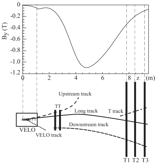
Figure 1: Track-type definitions in the LHCb tracking system. The main $B$-field component, along the $y$ direction, is plotted above as a function of the $z$ coordinate, along the beam axis. Figure taken from Ref. [50].

The tracking algorithms used for the reconstruction of Run 1 and Run 2 data are outlined in Refs. [49, 50], and briefly summarised below. For Run 3, the tracking algorithms have been updated to take full advantage of the upgraded tracker. However, the main features and especially the track definitions given above remain unchanged.

The search for Long tracks starts with identifying VELO hits that form straight line trajectories exploiting the negligibly small magnetic field in the VELO [56, 57, 58]. These tracks are reconstructed with a minimum of three hits in the $R$ sensors and three hits in the $\Phi$ sensors. There are two complementary algorithms to match VELO tracks with the hits in the TT and T1–T3 stations. In the first algorithm, called forward tracking [59], VELO tracks are combined with hits in the individual T stations that form clusters along the projected trajectory. In the second algorithm, a standalone track algorithm is used to reconstruct tracks using only the T1–T3 stations [60, 61] and assuming the tracks originate at the IP, which induces a small variation of the reconstruction efficiency as a function of the LLP decay position. Only track segments with at least one hit in the $x$ layer and one hit in the stereo layers ($u$ or $v$) for each T station are considered. VELO tracks are then combined with T track segments that provide the best possible match [62, 63]. Tracks reconstructed with either of the two algorithms are combined together. Finally, TT hits that are compatible with track extrapolations are added for improved momentum resolution.

Downstream tracks are reconstructed starting from T tracks, extrapolating them through the magnetic field and matching with TT hits [60, 64, 65]. Similarly, Upstream tracks are reconstructed by matching VELO tracks with residual hits in the TT stations. In both cases, for Upstream and Downstream tracks, at least three hits in the TT stations are required for the matching.

A fit based on the Kalman filter procedure [66, 67, 68, 69] is used on all tracks, using a fifth-order Runge-Kutta method [70, 71] to describe the track transport through the magnetic field, taking into account the material of the detector. After the fit, the reconstructed track is represented by a list of state vectors giving the transverse position, slopes with respect to the $z$ axis, and the charge/momentum ratio, $(x,y,{\rm d}x/{\rm d}z,{\rm d}y/{\rm d}z,q/p)$, specified at given $z$ positions in the experiment [72]. Duplicate tracks, known as clones, can occur when two or more tracks are reconstructed with the same trajectory and share most of their hits in the T and potentially TT stations. An algorithm, referred to as the clone killer, removes these tracks by only keeping the better track based on the total number of hits of the track and the goodness of the fit. Tracks involving more subdetectors are always preferred to individual segments. Therefore, T tracks are those that do not correspond to a Long or Downstream particle trajectory. No assumptions on the origin vertex of the track are made at this stage.

Fake tracks are those that are not associated to a real charged-particle trajectory, caused by random combinations of hits or mismatch of track segments upstream and downstream of the magnet. The fraction of fake Long tracks was estimated using Run 1 data to range from typically around $6.5$% in minimum bias events up to about $20$% for events with large track multiplicity [50]. This fake rate is significantly reduced in Run 2 by about 60% with a small drop in efficiency through a neural-network algorithm that uses information from the overall $\chi^{2}$ of the Kalman filter, the $\chi^{2}$ values of the track segments, the number of hits in the different detectors, and the $p_{T}$ of the track [73, 74]. Studies on simulated data estimate that around 5% of T tracks are fake due to detector hits caused by noise [3].

The ${{\mathchar 28931\relax}^{0}_{b}}\rightarrow{{J\mskip-3.0mu/\mskip-2.0mu\psi}}{\mathchar 28931\relax}$ and ${{B}^{0}}\rightarrow{{J\mskip-3.0mu/\mskip-2.0mu\psi}}{{K}^{0}_{\mathrm{S}}}$, with ${{J\mskip-3.0mu/\mskip-2.0mu\psi}}\rightarrow{\mu^{+}}{\mu^{-}}$, ${\mathchar 28931\relax}\rightarrow{p}{{\pi}^{-}}$ and ${{K}^{0}_{\mathrm{S}}}\rightarrow{{\pi}^{+}}{{\pi}^{-}}$ decays have been chosen as benchmark channels to study the capability and the performance of the LHCb detector in reconstructing LLPs using T tracks. The ${\mathchar 28931\relax}^{0}_{b}$ (and ${B}^{0}$) hadron has a characteristic flight length of around 10 mm, thus decaying inside the VELO detector. Muons are reconstructed as Long tracks, providing a precise determination of their momenta and of the ${J\mskip-3.0mu/\mskip-2.0mu\psi}$ decay vertex, which coincides with the decay vertex of the ${\mathchar 28931\relax}^{0}_{b}$ (${B}^{0}$) hadron, and allowing for kinematic constraints to be applied on the remaining part of the decay chain. The $\mathchar 28931\relax$ (${K}^{0}_{\mathrm{S}}$) decay candidates are reconstructed as combinations of two T tracks with their vertex position along the beam axis between 6.0 and 7.6 m from the nominal IP. Hadrons decaying in this region have traversed most of the magnetic field, thereby experiencing maximal spin precession, and their final-state particles reach the T1–T3 stations. The selection is based on the inclusive detached ${J\mskip-3.0mu/\mskip-2.0mu\psi}$ trigger, which is part of the LHCb trigger strategy in the Run 1 and Run 2 data-taking campaigns [54]. The events used correspond to an integrated luminosity of about $6$$\text{\,fb}^{-1}$ collected during Run 2.

Samples of simulated events are required to model the detector acceptance, detector response, reconstruction efficiency, and the effect of imposed signal selection requirements. Furthermore, the simulated events are used to train a classifier to discriminate between signal and background. In the simulation, $pp$ collisions are generated using Pythia [75] with a specific LHCb configuration [76]. Decays of unstable particles are described by EvtGen [77], in which final-state radiation is generated using Photos [78]. The transport of the generated particles and the detector response are implemented using the Geant4 toolkit [79], as described in Ref. [80].

5 Reconstruction of $\boldsymbol{{{\mathchar 28931\relax}^{0}_{b}}\rightarrow{{J\mskip-3.0mu/\mskip-2.0mu\psi}}{\mathchar 28931\relax}}$ decays

The reconstruction of the decay vertices of $\mathchar 28931\relax$ baryons decaying downstream of the TT (UT) stations presents two main challenges. Firstly, the particle trajectories must often be extrapolated over large distances through the strong and inhomogeneous magnetic field, accounting for effects induced by the particle interactions with air and detector material, using measurements only available downstream of the magnet (the T tracks). The uncertainty on the extrapolation depends on the measurement precision of the track slopes (${\rm d}x/{\rm d}z$ and ${\rm d}y/{\rm d}z$ parameters introduced in Sec. 4), which itself depends on the hit resolutions of the T1–T3 stations, and the precision and granularity of the magnetic field measurements. Therefore, the trajectories are influenced in a way that cannot be described by an exact analytical solution. Secondly, the measurement of particle momentum ($q/p$ parameter) relies on the relatively low curvature of T tracks, as they are reconstructed using hits located in a region with a weak magnetic field. As a consequence, the momentum resolution of T tracks is poor compared to Long or Downstream tracks, and the charge can be assigned incorrectly. In simulation about 0.5% of the T tracks have a wrong charge assignment.

The ${{\mathchar 28931\relax}^{0}_{b}}\rightarrow{{J\mskip-3.0mu/\mskip-2.0mu\psi}}{\mathchar 28931\relax}$ with ${\mathchar 28931\relax}\rightarrow{p}{{\pi}^{-}}$ signal candidates are first required to pass the online event selection performed by the detached ${{J\mskip-3.0mu/\mskip-2.0mu\psi}}\rightarrow{\mu^{+}}{\mu^{-}}$ trigger [54]. The offline selection involves a loose selection after the decay chain reconstruction, followed by a multivariate classifier based on a Histogrammed Gradient Boosted Decision Tree (HBDT) available in the scikit-learn package [81].

5.1 Signal candidate reconstruction and loose selection

Signal candidates are reconstructed following a two-stage procedure. First, decay vertices are reconstructed from the final-state particles using an iterative algorithm based on a Kalman filter [67, 69], referred to in the following as vertex fitter. The original track-state vectors are transformed, after transportation to the estimated vertex position of the previous iteration, into a convenient representation $(x,y,z,p_{x},p_{y},p_{z},E)$, where $E$ is the particle energy corresponding to momentum vector $(p_{x},p_{y},p_{z})$ at position $(x,y,z)$ for a given mass hypothesis [72]. The prior (seeding) covariance matrix of the vertex position is set to a large diagonal matrix, which removes any dependence on its prior knowledge. The convergence criterion is that between two consecutive iterations either the vertex position moves by less then 1$\,\upmu\text{m}$ or the $\chi^{2}$ changes by less than 0.01. The maximum number of iterations is 10. Since the ${{\mathchar 28931\relax}^{0}_{b}}\rightarrow{{J\mskip-3.0mu/\mskip-2.0mu\psi}}{\mathchar 28931\relax}$ with ${{J\mskip-3.0mu/\mskip-2.0mu\psi}}\rightarrow{\mu^{+}}{\mu^{-}}$ and ${\mathchar 28931\relax}\rightarrow{p}{{\pi}^{-}}$ decay chain involves multiple decays in cascade, these are reconstructed one-by-one using a bottom-up approach. In the second stage, the identified cascade decays are fed into a separate fitter, referred to as Decay Tree Fitter (DTF) [82], also based on a Kalman filter, where the whole decay chain is fitted simultaneously with kinematic constraints also imposed as appropriate.

In order to find a decay vertex position, tracks must be extrapolated during the Kalman filtering iterative procedure to a common vertex location. This step is particularly challenging for T tracks, as outlined above. For this task an approach based on a fifth-order Runge-Kutta method [70, 71] is employed instead of the default cubic interpolation of the track trajectory.

The loose selection criteria to identify signal candidates are based on the following variables: $p$ and $p_{T}$ of the proton, pion and $\mathchar 28931\relax$ candidates; the invariant masses of the ${\mu^{+}}{\mu^{-}}$, ${p}{{\pi}^{-}}$ and ${{J\mskip-3.0mu/\mskip-2.0mu\psi}}{\mathchar 28931\relax}$ systems; the vertex position along the $z$ axis of the $\mathchar 28931\relax$ candidate ($z_{\rm vtx}^{{\mathchar 28931\relax}}$); the cosine of the angle $\xi_{p}$ between the proton and the $\mathchar 28931\relax$ and ${\mathchar 28931\relax}^{0}_{b}$ momenta; the $\chi^{2}_{\rm IP}$ and $\chi^{2}_{\rm vtx}$ of the $\mathchar 28931\relax$ and ${\mathchar 28931\relax}^{0}_{b}$ candidates, where $\chi^{2}_{\rm IP}$ is the difference in the vertex-fit $\chi^{2}$ of the PV candidate reconstructed with and without the particle considered, and $\chi^{2}_{\rm vtx}$ is the decay vertex-fit $\chi^{2}$. In Table 1 of Appendix A, the loose selection requirements applied on these variables are summarised. All the subsequent analysis steps are performed using this selected sample.

Figure 2 shows the invariant-mass distributions of the ${p}{{\pi}^{-}}$ and ${{J\mskip-3.0mu/\mskip-2.0mu\psi}}{\mathchar 28931\relax}$ systems, $m({p}{{\pi}^{-}})$ and $m({{J\mskip-3.0mu/\mskip-2.0mu\psi}}{\mathchar 28931\relax})$, for simulated ${{\mathchar 28931\relax}^{0}_{b}}\rightarrow{{J\mskip-3.0mu/\mskip-2.0mu\psi}}{\mathchar 28931\relax}$ signal events. The ${{J\mskip-3.0mu/\mskip-2.0mu\psi}}{\mathchar 28931\relax}$ invariant mass is computed constraining the $b$-hadron candidate to originate at the PV, and the ${J\mskip-3.0mu/\mskip-2.0mu\psi}$ and $\mathchar 28931\relax$ masses to their known values [83]. The ${p}{{\pi}^{-}}$ invariant mass is evaluated without the $\mathchar 28931\relax$ mass constraint. The distributions are adequately described with an asymmetric and a symmetric double-tail Crystal Ball function [84], for the $m({p}{{\pi}^{-}})$ and $m({{J\mskip-3.0mu/\mskip-2.0mu\psi}}{\mathchar 28931\relax})$ distributions, respectively. The reconstructed sample amounts to about $31\,000$ signal events, from which a core invariant mass resolution of $6.8\pm 0.3$ and $37\pm 1$$\text{\,Me\kern-1.00006ptV\!/}c^{2}$ is obtained for $m({p}{{\pi}^{-}})$ and $m({{J\mskip-3.0mu/\mskip-2.0mu\psi}}{\mathchar 28931\relax})$, respectively, where the uncertainties are statistical.

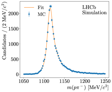
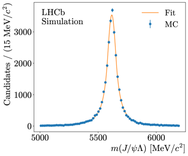
Figure 2: Invariant-mass distribution (left) $m({p}{{\pi}^{-}})$ and (right) $m({{J\mskip-3.0mu/\mskip-2.0mu\psi}}{\mathchar 28931\relax})$ for simulated ${{\mathchar 28931\relax}^{0}_{b}}\rightarrow{{J\mskip-3.0mu/\mskip-2.0mu\psi}}{\mathchar 28931\relax}$ signal decays. Blue points with error bars represent the Monte Carlo (MC) simulated data, and the overlaid (orange) curves are the projections of the mass fits.

The ${{B}^{0}}\rightarrow{{J\mskip-3.0mu/\mskip-2.0mu\psi}}{{K}^{0}_{\mathrm{S}}}$ with ${{K}^{0}_{\mathrm{S}}}\rightarrow{{\pi}^{+}}{{\pi}^{-}}$ decay constitutes a large source of physical background since the topology of the decay is almost identical to the signal, with the substitution of a proton by a pion in the final state. Due to the unavailability of PID information for T tracks in the current analysis, this background cannot be easily discriminated. In Fig. 3 (left), the invariant-mass distribution of ${K}^{0}_{\mathrm{S}}$ candidates from simulated ${{B}^{0}}\rightarrow{{J\mskip-3.0mu/\mskip-2.0mu\psi}}{{K}^{0}_{\mathrm{S}}}$ decays is compared with the corresponding distribution of $\mathchar 28931\relax$ candidates from ${\mathchar 28931\relax}^{0}_{b}$ decays where the proton of the final state has assigned the pion-mass hypothesis. Due to the poor mass resolution, the two distributions are almost completely overlapping, and a veto based on this variable does not help. Nevertheless, Fig. 3 (right) shows that the $m({{J\mskip-3.0mu/\mskip-2.0mu\psi}}{{K}^{0}_{\mathrm{S}}})$ invariant mass discriminates between the two $b$-hadron decays. A veto on candidates with $m({{J\mskip-3.0mu/\mskip-2.0mu\psi}}{{K}^{0}_{\mathrm{S}}})$ in the range $\pm 70$$\text{\,Me\kern-1.00006ptV\!/}c^{2}$ around the known ${B}^{0}$ mass [83] is applied in the following, unless otherwise stated, retaining $87$% of the ${\mathchar 28931\relax}^{0}_{b}$ signal while rejecting $65$% of the ${B}^{0}$ decays. The possibility of using PID information from the RICH2 detector, located downstream of the T1–T3 stations, to identify protons for Run 3 and beyond is under development.

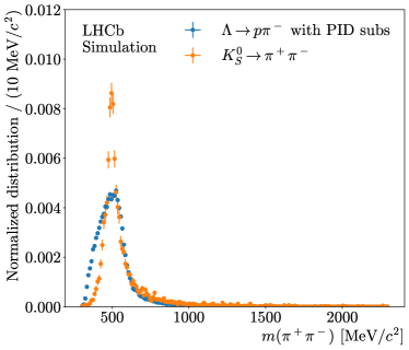
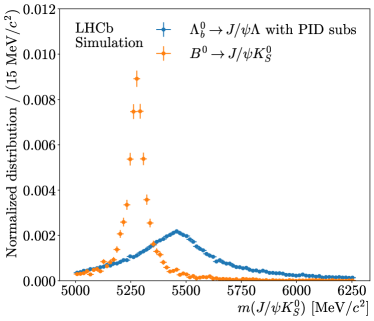
Figure 3: (Left) invariant-mass distribution $m({{\pi}^{+}}{{\pi}^{-}})$ of ${K}^{0}_{\mathrm{S}}$ candidates from simulated ${{B}^{0}}\rightarrow{{J\mskip-3.0mu/\mskip-2.0mu\psi}}{{K}^{0}_{\mathrm{S}}}$ decays (orange points) compared with the mass distribution of $\mathchar 28931\relax$ candidates from ${{\mathchar 28931\relax}^{0}_{b}}\rightarrow{{J\mskip-3.0mu/\mskip-2.0mu\psi}}{\mathchar 28931\relax}$ decays where the proton in the final state is assigned the pion-mass hypothesis (blue points). (Right) invariant-mass distribution $m({{J\mskip-3.0mu/\mskip-2.0mu\psi}}{{K}^{0}_{\mathrm{S}}})$ from simulated ${{B}^{0}}\rightarrow{{J\mskip-3.0mu/\mskip-2.0mu\psi}}{{K}^{0}_{\mathrm{S}}}$ decays (orange points) compared with the corresponding distribution from ${{\mathchar 28931\relax}^{0}_{b}}\rightarrow{{J\mskip-3.0mu/\mskip-2.0mu\psi}}{\mathchar 28931\relax}$ simulation where the proton in the final state has assigned the pion-mass hypothesis and the intermediate $\mathchar 28931\relax$ has assigned the ${K}^{0}_{\mathrm{S}}$-mass hypothesis (blue points).

5.2 Multivariate analysis for signal discrimination

A multivariate analysis is performed to enhance the signal purity. A Histogram-based Gradient Boosted Decision Tree (HBDT) classifier is used [81]. The training sample consists of about $43\,000$ simulated ${\mathchar 28931\relax}^{0}_{b}$ signal decays with about $6\times 10^{6}$ background candidates reconstructed on data. The background candidates are selected in the lower and upper sidebands of the $m({{J\mskip-3.0mu/\mskip-2.0mu\psi}}{\mathchar 28931\relax})$ distribution, defined by a $150$ and $300$$\text{\,Me\kern-1.00006ptV\!/}c^{2}$ wide window below and above a signal region $\pm 600$$\text{\,Me\kern-1.00006ptV\!/}c^{2}$ around the known ${\mathchar 28931\relax}^{0}_{b}$ mass [83]. The training is performed using $90$% of the sample, while the remaining $10$% is held out for the assessment of the classifier performance. The classifier includes kinematic and topological variables: the longitudinal and transverse momenta of the proton, pion and ${J\mskip-3.0mu/\mskip-2.0mu\psi}$ candidates; the coordinates of the $\mathchar 28931\relax$ decay vertex, $(x,y,z)_{\rm vtx}^{\mathchar 28931\relax}$; the cosine of the angle between the momentum and the flight direction of the $\mathchar 28931\relax$ and ${\mathchar 28931\relax}^{0}_{b}$ decaying particles; the $\chi^{2}_{\rm vtx}$, $\chi^{2}_{\rm IP}$ and $\chi^{2}_{\rm dist}$ of the $\mathchar 28931\relax$ and ${\mathchar 28931\relax}^{0}_{b}$ candidates, where $\chi^{2}_{\rm dist}$ is the squared distance between the PV and the particle decay vertex normalised to its uncertainty; and the status flags (converged/failed) of the decay chain vertex fit with and without the $\mathchar 28931\relax$ mass constraint.

The following hyperparameters of the HBDT are optimised: the maximum number of leaf nodes for the decision trees; the learning rate, i.e. the weight applied to each successive decision tree of the boosting procedure; and the total number of iterations (number of decision trees in the ensemble). The performance of the trained HBDT is estimated calculating the Area-Under-Curve (AUC) of the curve representing the signal purity versus the signal efficiency, with the threshold applied to the HBDT response varying continuously from zero to one.

The operating point is set applying a threshold of $0.366$ to the HBDT response, and is chosen by optimising the significance $S/\sqrt{S+B}$ as a function of the HBDT threshold, where $S$ and $B$ are the signal and background yields in the signal region, respectively. For this purpose, the significance is estimated for each HBDT threshold performing a binned fit to the ${{\mathchar 28931\relax}^{0}_{b}}\rightarrow{{J\mskip-3.0mu/\mskip-2.0mu\psi}}{\mathchar 28931\relax}$ invariant-mass distribution on data. Training the classifier with a similar size of the signal and background proxies induces a shift of the optimal threshold with no impact on the significance.

5.3 Armenteros-Podolanski plot

The Armenteros-Podolanski (AP) plot [85] can be used as a kinematics-based PID technique to reject ${K}^{0}_{\mathrm{S}}$ background events from the $\mathchar 28931\relax$ and ${{\mathchar 28931\relax}^{0}_{b}}\rightarrow{{J\mskip-3.0mu/\mskip-2.0mu\psi}}{\mathchar 28931\relax}$ samples. For two-body decays of a particle of mass $M$ into two particles of masses $m_{1}$ and $m_{2}$, it is a representation of the transverse momentum versus the asymmetry of the longitudinal momenta of the final-state particles with respect to the parent flight direction. In this diagram, the decays show as a semiellipse centered at $((m_{1}^{2}-m_{2}^{2})/M^{2},0)$ and with radii $(2p_{\rm cm}/M,p_{\rm cm})$, where $p_{\rm cm}$ is the momentum of the child particles in the parent centre-of-mass frame.

Figure 4 shows the AP plot for ${{\mathchar 28931\relax}^{0}_{b}}\rightarrow{{J\mskip-3.0mu/\mskip-2.0mu\psi}}{\mathchar 28931\relax}$ signal compared to ${{B}^{0}}\rightarrow{{J\mskip-3.0mu/\mskip-2.0mu\psi}}{{K}^{0}_{\mathrm{S}}}$ signal from simulation, and ${{\mathchar 28931\relax}^{0}_{b}}\rightarrow{{J\mskip-3.0mu/\mskip-2.0mu\psi}}{\mathchar 28931\relax}$ Run 2 data, from the decay chain vertex fit with the ${J\mskip-3.0mu/\mskip-2.0mu\psi}$ mass constraint and after the loose, HBDT and ${B}^{0}$ veto selection criteria applied. The depleted central region of the ${K}^{0}_{\mathrm{S}}$ semiellipse in the data reveals that the HBDT requirement, combined with the ${B}^{0}$ veto, is effectively removing ${K}^{0}_{\mathrm{S}}$ background events not overlapping with the $\mathchar 28931\relax$ and $\kern 1.79993pt\overline{\kern-1.79993pt\mathchar 28931\relax}$ semiellipses. This is due to the inclusion of the transverse and longitudinal momenta of the proton and pion from the $\mathchar 28931\relax$ decay in the classifier. Requiring the magnitude of the longitudinal momentum asymmetry to exceed 0.5 rejects 17% of the remaining ${B}^{0}$ decays, with a signal efficiency of 99%, for candidates passing all selection criteria including the ${B}^{0}$ veto. The requirement, applied hereafter unless otherwise specified, removes 7% of the selected candidates on data.

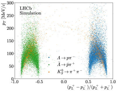
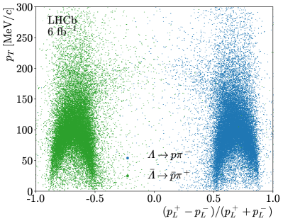
Figure 4: The AP plot for (left) simulated ${{\mathchar 28931\relax}^{0}_{b}}\rightarrow{{J\mskip-3.0mu/\mskip-2.0mu\psi}}{\mathchar 28931\relax}$ and ${{B}^{0}}\rightarrow{{J\mskip-3.0mu/\mskip-2.0mu\psi}}{{K}^{0}_{\mathrm{S}}}$ signal events reconstructed as ${{\mathchar 28931\relax}^{0}_{b}}\rightarrow{{J\mskip-3.0mu/\mskip-2.0mu\psi}}{\mathchar 28931\relax}$ decays and (right) ${{\mathchar 28931\relax}^{0}_{b}}\rightarrow{{J\mskip-3.0mu/\mskip-2.0mu\psi}}{\mathchar 28931\relax}$ Run 2 data, after the loose, HBDT and ${B}^{0}$ veto selection criteria. The symbol $p_{L}^{+}$ ($p_{L}^{-}$) refers to the longitudinal momentum of the positively (negatively) charged final-state particle, i.e. the $p$ and ${\pi}^{+}$ (${\pi}^{-}$ and $\overline{p}$) in the $\mathchar 28931\relax$ and $\kern 1.61993pt\overline{\kern-1.61993pt\mathchar 28931\relax}$ decay, respectively, and $p_{T}$ their transverse momentum, calculated with respect to the hyperon flight direction.

5.4 Reconstruction efficiency and resolutions

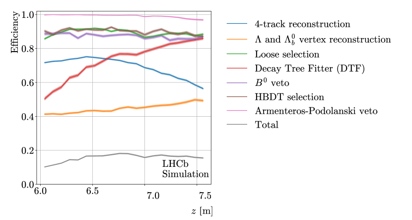
Figure 5: Reconstruction efficiency as a function of the true $\mathchar 28931\relax$ decay vertex position along the beam axis for simulated ${{\mathchar 28931\relax}^{0}_{b}}\rightarrow{{J\mskip-3.0mu/\mskip-2.0mu\psi}}{\mathchar 28931\relax}$ signal events (grey) and its breakdown for different reconstruction steps: the reconstruction and quality selections of the four tracks of the final state (blue); the reconstruction of the $\mathchar 28931\relax$ and ${\mathchar 28931\relax}^{0}_{b}$ decay vertices (orange); the initial selections applied to the daughter and reconstructed decay candidates as described in Table 1 (Appendix A, green); the fraction of successful decay chain vertex fits (DTF, red); the ${B}^{0}$ mass veto (violet); the selection efficiency of the HBDT (maroon); and the AP veto (pink). The four-track efficiency contribution and the total efficiency (see text) are evaluated for reconstructible signal decays, while all other contributions are relative to the previous reconstruction step.

The reconstruction efficiency is defined here as the probability that a reconstructible ${{\mathchar 28931\relax}^{0}_{b}}\rightarrow{{J\mskip-3.0mu/\mskip-2.0mu\psi}}{\mathchar 28931\relax}$ signal decay, with all their final-state trajectories (i.e., four tracks) within the LHCb detector acceptance and intersecting the minimum detector elements required for each track type [49, 55] outlined in Sec. 4, is actually reconstructed. Signal decays with $\mathchar 28931\relax$ decaying in the region between 6.0 and 7.6 m represent 4% of all generated events and have a reconstructibility of 59% and a four-track reconstruction efficiency of 70%. Overall, this represents about 8% of all reconstructible and four-track reconstructed decays (see Appendix C for further details). Figure 5 shows the reconstruction efficiency and its breakdown for the different reconstruction steps as a function of the true $\mathchar 28931\relax$ decay vertex position along the beam axis. The efficiency is about $8$% at $6.0$ m from the IP; it rises to about $16$% at $6.8$ m; then it decreases slightly staying above $13$% between $7.0$ and $7.6$ m. The reconstruction of the $\mathchar 28931\relax$ and ${\mathchar 28931\relax}^{0}_{b}$ vertices fails in more than $50$% of the cases, with a slightly larger success rate when the $\mathchar 28931\relax$ baryon decays closer to the T stations (see Fig. 1). The efficiency of the loose selection is about $90$%, mostly independent of the $\mathchar 28931\relax$ decay location. The decay chain vertex fit convergence depends on the $\mathchar 28931\relax$ decay vertex position, going from about $50$% for $\mathchar 28931\relax$ baryons decaying farthest from the T stations, to about $86$% for those closest to them. This highlights the impact of the propagation of T tracks through the magnetic field. The HBDT and AP veto selection efficiencies are about $72$% and $99\%$, largely independent of the position of the $\mathchar 28931\relax$ decay vertex.

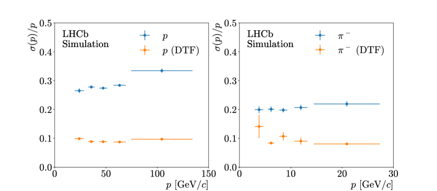
Figure 6: Relative momentum resolution as a function of the (left) proton and (right) pion momentum reconstructed as final states of the ${{\mathchar 28931\relax}^{0}_{b}}\rightarrow{{J\mskip-3.0mu/\mskip-2.0mu\psi}}{\mathchar 28931\relax}$ decay chain. The track fit resolution before (blue points) and after (orange points) the decay chain vertex fit is compared.

The momentum resolution of T tracks suffers from the lack of a high magnetic field in the region where the trajectories are reconstructed, resulting in a large bending radius. Figure 6 shows that the momentum resolution improves significantly when the kinematic constraints of the ${\mathchar 28931\relax}^{0}_{b}$ decay chain are taken into account, namely the ${J\mskip-3.0mu/\mskip-2.0mu\psi}$ and $\mathchar 28931\relax$ mass constraints. The relative resolution from the track fits is about $30$% and $20$% for the proton and the pion, respectively. The resolution improves to about $10$% for both particles with the kinematic constraints applied.

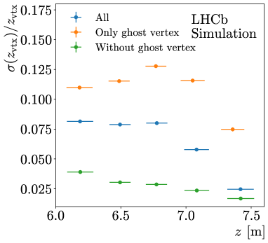
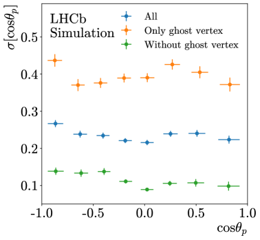
Figure 7: (Left) relative precision of the $\mathchar 28931\relax$ decay vertex position along the beam axis and (right) resolution of the cosine of the proton helicity angle from the decay chain vertex fit. Blue points with error bars are for all events. The corresponding resolutions for events with or without a ghost vertex (see text) are also shown with orange or green points, respectively.

The reconstruction of the $\mathchar 28931\relax$ decay vertex using T tracks is particularly challenging when the vertex position is located far from the T1–T3 tracking stations. Figure 7 (left) shows the relative precision of the $\mathchar 28931\relax$ vertex position along the beam axis, which is about $8$% for vertices reconstructed around $6.0$ m from the nominal IP; it becomes significantly better for vertices located closer to the T stations, around $7.5$ m, where it is about $2.5$%. Figure 7 (right) shows the absolute resolution of the cosine of the proton helicity angle, $\cos\theta_{p}$, defined as the angle between the proton direction in the rest frame of the $\mathchar 28931\relax$ reached from the ${\mathchar 28931\relax}^{0}_{b}$ rest frame and the $\mathchar 28931\relax$ direction in the rest frame of the ${\mathchar 28931\relax}^{0}_{b}$. This variable is an essential ingredient of the $\mathchar 28931\relax$-polarisation determination required for the MDM and EDM measurements [17]. The average resolution is about $0.25$. Figure 19 (left) in Appendix B shows the corresponding detector-response matrix.

These relatively poor resolutions are in fact not exclusively due to the lack of high magnetic field and the long track-transportation distances. Events with the closing-track topology sketched in Fig. 8 (left), referred to hereafter as ‘ghost’ events, exhibit particle trajectories with two (consistent within track uncertainties) crossing points, inducing the vertex fitter to converge frequently to the ghost vertex. In contrast, opening-track events, shown in Fig. 8 (right), do not have a ghost vertex and converge to the correct position.

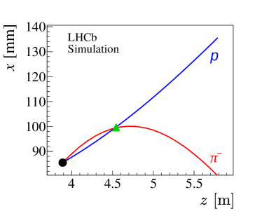
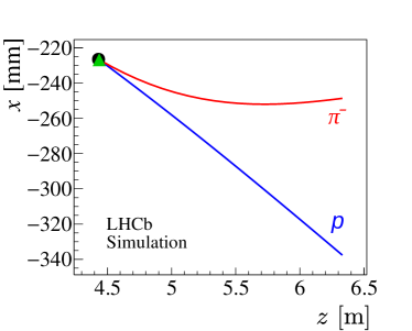
Figure 8: Event displays with (blue) proton and (red) pion trajectories together with true vertex (black dot or green triangle) and the reconstructed vertex (green triangle or black dot) for typical events from the simulation. The reconstructed vertex is wrongly assigned to the downstream (larger $z$) crossing point between particle trajectories in most of the events with closing-track topology (left), while it is found correctly in opening-track topologies (right).

Closing- and opening-track geometries can be identified through two kinematic variables, illustrated in Fig. 9. The horizontality, $h$, is defined as the $y$ component (along the normal to the bending $xz$ plane) of the unit decay-plane vector times the product of the proton/antiproton charge and the dipole magnet polarity. The second variable, $\psi$, is the angle between the true and reconstructed decay planes, and thus can only be determined for simulation. A strong correlation is observed between the true $h$ and $\psi$ for closing-track topology, $h<0$, as shown in Fig. 10 (left), where the $\mathchar 28931\relax$ decay vertex is incorrectly reconstructed and associated to the ghost crossing point (also referred to as ghost events). This results in a sizeable vertex bias and a strong vertex resolution degradation for ghost events, as illustrated in Fig. 10 (right) and Fig. 7 (left), respectively. About 30% of the reconstructed decays are ghosts. For events without a ghost vertex, the average helicity angle resolution improves by a factor $2.5$ reaching $0.10$. Selecting events with positive reconstructed $h$ removes the ghost events and thus most of the observed bias and resolution degradation, at the cost of a low efficiency of about 20%.

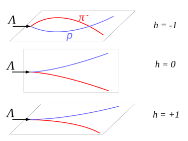
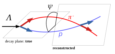
Figure 9: (Left) schematic representation of events with limiting values of true horizontality $h$ and (right) definition of $\psi$ as the angle between the true and the reconstructed decay planes.

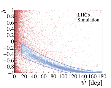
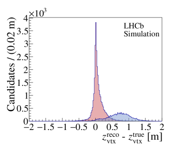
Figure 10: (Left) distribution of true horizontality and $\psi$ for signal ${{\mathchar 28931\relax}^{0}_{b}}\rightarrow{{J\mskip-3.0mu/\mskip-2.0mu\psi}}{\mathchar 28931\relax}$ simulated events and (right) residual of the reconstructed vertex $z$ position for events with true $\mathchar 28931\relax$ vertex along the $z$ axis above 6.0 m, before selection criteria. A strong correlation between $h$ and $\psi$ arises for events with closing-track topologies, $h<0$, for which the $\mathchar 28931\relax$ decay vertex is wrongly assigned to the ghost crossing point. By selecting events between the blue lines, where the vast majority of the closing-track events with reconstructed ghost vertex are present (amounting to about 30% of all events), the dominant source of the bias on the vertex $z$ position is clearly identified.

5.5 Results on data

Figure 11 shows the $m({p}{{\pi}^{-}})$ and $m({{J\mskip-3.0mu/\mskip-2.0mu\psi}}{\mathchar 28931\relax})$ distributions of the selected ${{\mathchar 28931\relax}^{0}_{b}}\rightarrow{{J\mskip-3.0mu/\mskip-2.0mu\psi}}{\mathchar 28931\relax}$ candidates from Run 2 data, after all selection criteria and applying the decay chain vertex fit. Signal and background yields along with the invariant-mass resolutions are obtained by fitting these distributions independently. The signal components are adequately described with asymmetric and symmetric double-tail Crystal Ball functions [84], respectively, with tail parameters in the latter fixed to the values obtained from the fit to the simulated signal events shown in Fig. 2. The background from ${K}^{0}_{\mathrm{S}}$ decays in the $m({p}{{\pi}^{-}})$ distribution is parameterised using a template determined from simulated ${{B}^{0}}\rightarrow{{J\mskip-3.0mu/\mskip-2.0mu\psi}}{{K}^{0}_{\mathrm{S}}}$ decays, and there is no evidence of combinatorial background. Instead, the background contribution to the $m({{J\mskip-3.0mu/\mskip-2.0mu\psi}}{\mathchar 28931\relax})$ distribution is largely dominated by random combinations of ${J\mskip-3.0mu/\mskip-2.0mu\psi}$ and $\mathchar 28931\relax$ candidates, with a residual contribution from ${{B}^{0}}\rightarrow{{J\mskip-3.0mu/\mskip-2.0mu\psi}}{{K}^{0}_{\mathrm{S}}}$ decays, and is modelled with an exponential function. The resulting fits yield about $43\,500$ ${\mathchar 28931\relax}\rightarrow{p}{{\pi}^{-}}$ and $6\,140$ ${{\mathchar 28931\relax}^{0}_{b}}\rightarrow{{J\mskip-3.0mu/\mskip-2.0mu\psi}}{\mathchar 28931\relax}$ signal decays, with core mass resolutions of $7.7\pm 0.4$ and $41\pm 2$$\text{\,Me\kern-1.00006ptV\!/}c^{2}$, respectively, about 10% worse than in simulation. The ${K}^{0}_{\mathrm{S}}$ background is determined to be about $15\,000$ events in the full $m({p}{{\pi}^{-}})$ range shown in Fig. 11 (left), whereas the background yield in the $m({{J\mskip-3.0mu/\mskip-2.0mu\psi}}{\mathchar 28931\relax}$) distribution, estimated in a region defined by three times the invariant mass resolution around the mean mass, amounts to $10\,800$.

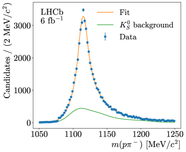
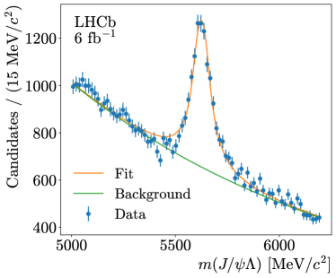
Figure 11: Invariant-mass distribution (left) $m({p}{{\pi}^{-}})$ and (right) $m({{J\mskip-3.0mu/\mskip-2.0mu\psi}}{\mathchar 28931\relax})$ for ${{\mathchar 28931\relax}^{0}_{b}}\rightarrow{{J\mskip-3.0mu/\mskip-2.0mu\psi}}{\mathchar 28931\relax}$ candidates reconstructed using Run 2 data after all selection criteria. The projections of the mass fits are overlaid.

6 Reconstruction of $\boldsymbol{{{B}^{0}}\rightarrow{{J\mskip-3.0mu/\mskip-2.0mu\psi}}{{K}^{0}_{\mathrm{S}}}}$ decays

A sample of long-lived ${K}^{0}_{\mathrm{S}}$ mesons from ${{B}^{0}}\rightarrow{{J\mskip-3.0mu/\mskip-2.0mu\psi}}{{K}^{0}_{\mathrm{S}}}$ decays is also reconstructed using a similar procedure to that described in Sec. 5 for ${{\mathchar 28931\relax}^{0}_{b}}\rightarrow{{J\mskip-3.0mu/\mskip-2.0mu\psi}}{\mathchar 28931\relax}$ decays. The loose selection criteria to identify ${B}^{0}$ candidates are summarised in Table 2 of Appendix A.

Due to the similar topologies and the lack of PID information, ${{\mathchar 28931\relax}^{0}_{b}}\rightarrow{{J\mskip-3.0mu/\mskip-2.0mu\psi}}{\mathchar 28931\relax}$ decays represent a physical background for the reconstruction of ${{B}^{0}}\rightarrow{{J\mskip-3.0mu/\mskip-2.0mu\psi}}{{K}^{0}_{\mathrm{S}}}$ events. A veto is applied to reject candidates with $m({{J\mskip-3.0mu/\mskip-2.0mu\psi}}{\mathchar 28931\relax})$ in the range $\pm 150$$\text{\,Me\kern-1.00006ptV\!/}c^{2}$ around the known ${\mathchar 28931\relax}^{0}_{b}$ mass [83], where the positive pion from the ${K}^{0}_{\mathrm{S}}$ candidate is reconstructed with the proton mass hypothesis. This results in a $96$% selection efficiency for the ${B}^{0}$ signal and $37$% for the ${\mathchar 28931\relax}^{0}_{b}$ background. Similarly to the reconstruction of ${{\mathchar 28931\relax}^{0}_{b}}\rightarrow{{J\mskip-3.0mu/\mskip-2.0mu\psi}}{\mathchar 28931\relax}$ decays, an HBDT classifier has been trained using about 22 000 simulated ${B}^{0}$ signal decays and about $6\times 10^{6}$ background candidates reconstructed on data and selected from the lower and upper sidebands of the $m({{J\mskip-3.0mu/\mskip-2.0mu\psi}}{{K}^{0}_{\mathrm{S}}})$ distribution. A threshold of 0.0228 to the HBDT response is chosen by optimising the signal significance. Requiring further the longitudinal momentum asymmetry in the ${{B}^{0}}\rightarrow{{J\mskip-3.0mu/\mskip-2.0mu\psi}}{{K}^{0}_{\mathrm{S}}}$ AP plot, shown in Fig. 12 for simulation and data, to be within $\pm 0.5$, rejects 99% of the ${{\mathchar 28931\relax}^{0}_{b}}\rightarrow{{J\mskip-3.0mu/\mskip-2.0mu\psi}}{\mathchar 28931\relax}$ background while retaining 66% of the signal.

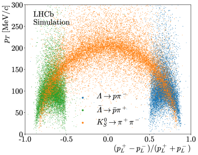
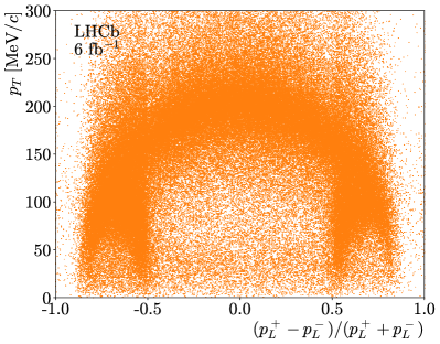
Figure 12: The AP plot for (left) simulated ${{\mathchar 28931\relax}^{0}_{b}}\rightarrow{{J\mskip-3.0mu/\mskip-2.0mu\psi}}{\mathchar 28931\relax}$ and ${{B}^{0}}\rightarrow{{J\mskip-3.0mu/\mskip-2.0mu\psi}}{{K}^{0}_{\mathrm{S}}}$ signal events reconstructed as ${{B}^{0}}\rightarrow{{J\mskip-3.0mu/\mskip-2.0mu\psi}}{{K}^{0}_{\mathrm{S}}}$ decays and (right) ${{B}^{0}}\rightarrow{{J\mskip-3.0mu/\mskip-2.0mu\psi}}{{K}^{0}_{\mathrm{S}}}$ candidates reconstructed on Run 2 data, after the loose, HBDT and ${\mathchar 28931\relax}^{0}_{b}$ veto selection criteria.

The total reconstruction efficiency ranges from about $10$% for ${K}^{0}_{\mathrm{S}}$ decays taking place at $6.0$ m from the nominal IP to about $16$% when they occur closest to the T station, as illustrated in Fig. 13, along with the breakdown of the steps in the reconstruction sequence. We observe that the tracking and vertexing efficiencies are very similar to those obtained for the ${\mathchar 28931\relax}^{0}_{b}$ case (Fig. 5), while the decay chain vertex fit performance is slightly better. The lower efficiency of the loose selection is partially compensated by the higher efficiency of the HBDT selection. The total efficiency is lower than for ${\mathchar 28931\relax}^{0}_{b}$ decays due to the lower efficiency of the AP veto.

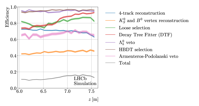
Figure 13: Reconstruction efficiency as a function of the true ${K}^{0}_{\mathrm{S}}$ decay vertex position along the beam axis for simulated ${{B}^{0}}\rightarrow{{J\mskip-3.0mu/\mskip-2.0mu\psi}}{{K}^{0}_{\mathrm{S}}}$ signal events (grey) and its breakdown for different reconstruction steps: the reconstruction and quality selections of the four tracks of the final state (blue); the reconstruction of the ${K}^{0}_{\mathrm{S}}$ and ${B}^{0}$ decay vertices (orange); the initial selection applied to the daughter and reconstructed decay candidates as described in Table 2 (Appendix A, green); the fraction of successful decay chain vertex fits (DTF, red); the ${\mathchar 28931\relax}^{0}_{b}$ mass veto (violet); the selection efficiency of the HBDT (maroon); and the AP veto (pink).

Figure 14 compares the momentum resolution of the two pions from the ${K}^{0}_{\mathrm{S}}$ decay with and without the kinematic constraints. Similarly to the ${\mathchar 28931\relax}^{0}_{b}$ case, the momentum resolution improves significantly when the kinematic constraints on the ${J\mskip-3.0mu/\mskip-2.0mu\psi}$ and ${K}^{0}_{\mathrm{S}}$ candidates are applied, reaching about $10$%. Figure 15 (left) shows the relative precision of the ${K}^{0}_{\mathrm{S}}$ vertex position along the $z$ axis for all events passing the selection criteria and separately for events with and without a ghost vertex. The combined resolution ranges from about $10$% at 6.0 m from the nominal IP to 2% close to the T stations, similarly to $\mathchar 28931\relax$ decays. Analogously, Fig. 15 (right) illustrates the corresponding absolute resolution of the cosine of the ${\pi}^{+}$ helicity angle, $\cos\theta_{{\pi}^{+}}$. The average resolution is about $0.07$, slightly better than for $\mathchar 28931\relax$ decays without a ghost vertex. Figure 19 (right) in Appendix B shows the corresponding detector-response matrix. In contrast to the ${\mathchar 28931\relax}^{0}_{b}$ case, only 1% of the selected candidates passing all selection criteria contain a ghost vertex, as can be seen in Fig. 16. The larger $Q$-value, defined as the mass difference between the initial and final-state particles, together with the equal masses of the final-state particles results in the majority of the events having an opening-track topology, similar to that sketched in Fig. 8 (right).

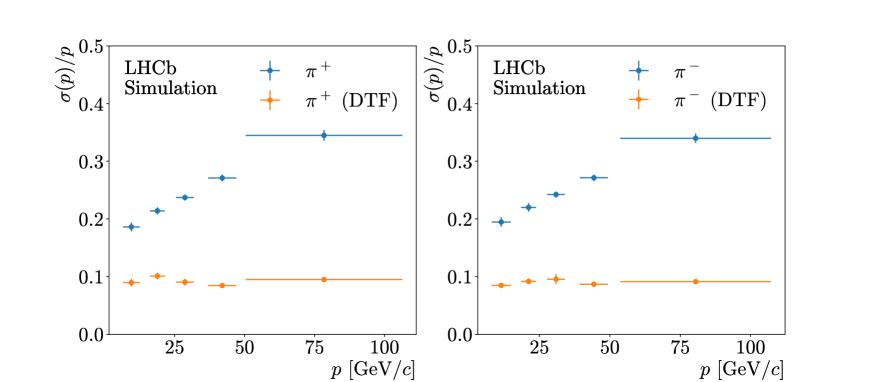
Figure 14: Relative momentum resolution as a function of the momentum of the (left) positively and (right) negatively charged pions reconstructed as final states of a ${B}^{0}$ decay chain. The track fit resolution before (blue) and after (orange) the decay chain vertex fit is compared.

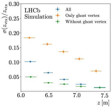
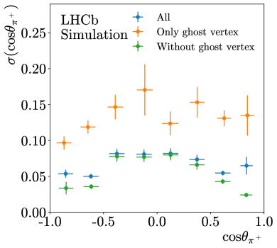
Figure 15: (Left) relative precision of the ${K}^{0}_{\mathrm{S}}$ vertex position along the beam axis. (Right) resolution of the cosine of the ${\pi}^{+}$ helicity angle from the decay chain vertex fit. Blue points with error bars are for all events. The corresponding resolutions for events with or without a ghost vertex are also shown with orange or green points, respectively.

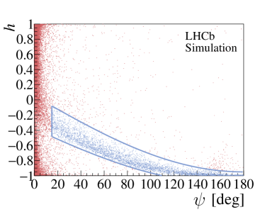
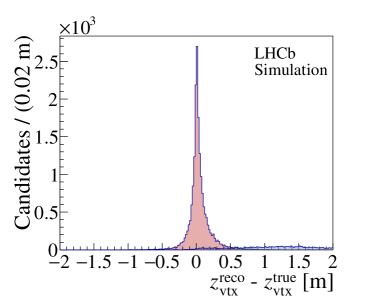
Figure 16: (Left) distribution of true horizontality and $\psi$ for simulated ${{B}^{0}}\rightarrow{{J\mskip-3.0mu/\mskip-2.0mu\psi}}{{K}^{0}_{\mathrm{S}}}$ events and (right) residual of the reconstructed vertex $z$ position for events with true ${K}^{0}_{\mathrm{S}}$ vertex along the $z$ axis above 6 m, before selection criteria. The strong correlation between $h$ and $\psi$ for events with closing-track topologies (blue region), which are the dominant source of vertex bias, occurs for 1% of the events after the loose, HBDT and veto selection criteria, and about 15% before.

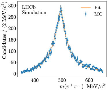
Figure 17: Invariant-mass distribution (left) $m({{\pi}^{+}}{{\pi}^{-}})$ and (right) $m({{J\mskip-3.0mu/\mskip-2.0mu\psi}}{{K}^{0}_{\mathrm{S}}})$ for simulated ${{B}^{0}}\rightarrow{{J\mskip-3.0mu/\mskip-2.0mu\psi}}{{K}^{0}_{\mathrm{S}}}$ signal decays. Blue points with error bars represent the MC simulated data, and the overlaid (orange) curves are the projections of the mass fits.

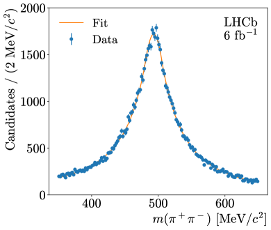
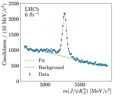
Figure 18: Invariant-mass distribution (left) $m({{\pi}^{+}}{{\pi}^{-}})$ and (right) $m({{J\mskip-3.0mu/\mskip-2.0mu\psi}}{{K}^{0}_{\mathrm{S}}})$ for ${{B}^{0}}\rightarrow{{J\mskip-3.0mu/\mskip-2.0mu\psi}}{{K}^{0}_{\mathrm{S}}}$ candidates using Run 2 data after all selection criteria. The projections of the mass fits are overlaid.

Figure 17 shows the $m({{\pi}^{+}}{{\pi}^{-}})$ and $m({{J\mskip-3.0mu/\mskip-2.0mu\psi}}{{K}^{0}_{\mathrm{S}}})$ distributions of the reconstructed and selected ${{B}^{0}}\rightarrow{{J\mskip-3.0mu/\mskip-2.0mu\psi}}{{K}^{0}_{\mathrm{S}}}$ candidates from simulation, about $13\,000$ in total, along with the mass fits. Figure 18 shows the corresponding distributions for ${B}^{0}$ candidates reconstructed on data after selection requirements. The signal shapes are modelled using an asymmetric double-tail Crystal Ball function [84], while the background contribution to the ${{B}^{0}}\rightarrow{{J\mskip-3.0mu/\mskip-2.0mu\psi}}{{K}^{0}_{\mathrm{S}}}$ invariant-mass distribution, of combinatorial nature, is described using an exponential function. A total of $120\,000$ ${K}^{0}_{\mathrm{S}}$ and $13\,300$ ${{B}^{0}}\rightarrow{{J\mskip-3.0mu/\mskip-2.0mu\psi}}{{K}^{0}_{\mathrm{S}}}$ signal events are reconstructed on data, with core mass resolutions of $20\pm 1$$\text{\,Me\kern-1.00006ptV\!/}c^{2}$ and $28\pm 1$$\text{\,Me\kern-1.00006ptV\!/}c^{2}$, respectively, which can be compared to $13\pm 3$$\text{\,Me\kern-1.00006ptV\!/}c^{2}$ and $29\pm 1$$\text{\,Me\kern-1.00006ptV\!/}c^{2}$ on simulation. The background yield in the $m({{J\mskip-3.0mu/\mskip-2.0mu\psi}}{{K}^{0}_{\mathrm{S}}}$) region, defined by three times the invariant-mass resolution, amounts to $13\,200$.

7 Conclusions and prospects

The reconstruction of long-lived particles decaying downstream of the dipole magnet is proved to be possible with the LHCb detector. Samples of $\mathchar 28931\relax$ and ${K}^{0}_{\mathrm{S}}$ hadrons from ${{\mathchar 28931\relax}^{0}_{b}}\rightarrow{{J\mskip-3.0mu/\mskip-2.0mu\psi}}{\mathchar 28931\relax}$ and ${{B}^{0}}\rightarrow{{J\mskip-3.0mu/\mskip-2.0mu\psi}}{{K}^{0}_{\mathrm{S}}}$ decays, with the vertex position between 6.0 and 7.6 m away from the IP, have been reconstructed using data recorded by LHCb during the LHC Run 2, corresponding to an integrated luminosity of about 6$\text{\,fb}^{-1}$. Due to the long extrapolation distances across the magnet region, the vertex reconstruction using tracks with hits only in the tracking stations downstream of the dipole magnet requires an accurate track transporter based on the Runge-Kutta method instead of the usual polynomial approximation. The experimental resolution largely benefits from the geometric and kinematic constraints of the decay chain when the long-lived particles are produced from exclusive $b$-hadron decays. In addition, the combined use of a multivariate classifier with the Armenteros-Podolanski technique maximises the selection performance and mitigates cross-feed from other long-lived decays.

For the future, several improvements to the reconstruction and selection of long-lived particles using T tracks are possible. These include the addition of PID information based on measurements from the RICH detector located downstream of the last T stations, optimisation of the Kalman filtering for T tracks, and adaptation of vertexing algorithms to enhance the reconstruction efficiency and to mitigate biases mostly induced by closing-track event topologies. Furthermore, the implementation of dedicated trigger lines will become available with the more flexible software-based trigger of the LHCb upgraded detector. The trigger, reconstruction and selection of LLPs using T tracks will offer new opportunities to significantly extend the physics reach of the LHCb experiment through measurements of the magnetic and electric dipole moments of the $\mathchar 28931\relax$ baryon and searches for LLPs predicted by various BSM theories.

Appendix A Loose selection of $\boldsymbol{{{\mathchar 28931\relax}^{0}_{b}}\rightarrow{{J\mskip-3.0mu/\mskip-2.0mu\psi}}{\mathchar 28931\relax}}$ and $\boldsymbol{{{B}^{0}}\rightarrow{{J\mskip-3.0mu/\mskip-2.0mu\psi}}{{K}^{0}_{\mathrm{S}}}}$ decays

Tables 1 and 2 report the loose selection requirements applied to the ${{\mathchar 28931\relax}^{0}_{b}}\rightarrow{{J\mskip-3.0mu/\mskip-2.0mu\psi}}{\mathchar 28931\relax}$ and ${{B}^{0}}\rightarrow{{J\mskip-3.0mu/\mskip-2.0mu\psi}}{{K}^{0}_{\mathrm{S}}}$ with ${{J\mskip-3.0mu/\mskip-2.0mu\psi}}\rightarrow{\mu^{+}}{\mu^{-}}$, ${\mathchar 28931\relax}\rightarrow{p}{{\pi}^{-}}$ and ${{K}^{0}_{\mathrm{S}}}\rightarrow{{\pi}^{+}}{{\pi}^{-}}$ candidates passing the online event selection.

Table 1: Loose selection requirements applied to ${{\mathchar 28931\relax}^{0}_{b}}\rightarrow{{J\mskip-3.0mu/\mskip-2.0mu\psi}}{\mathchar 28931\relax}$ candidates passing the online event selection. The invariant masses $m(p{{\pi}^{-}})$ and $m({{J\mskip-3.0mu/\mskip-2.0mu\psi}}{\mathchar 28931\relax})$ are obtained from the vertex fitter.

Variable	Units	Minimum	Maximum
$p\,(\pi)$	$\text{\,Me\kern-1.00006ptV\!/}c$	$20\,00$	$500\,000$
$p\,(p)$	$\text{\,Me\kern-1.00006ptV\!/}c$	$10\,000$	$500\,000$
$p_{T}\,(p)$	$\text{\,Me\kern-1.00006ptV\!/}c$	$400$	$-$
$m(p\pi)$	$\text{\,Me\kern-1.00006ptV\!/}c^{2}$	$600$	$1\,500$
$z_{\rm vtx}^{{\mathchar 28931\relax}}$	mm	$5\,500$	$8\,500$
$\cos\xi_{p}\,({\mathchar 28931\relax})$		$0.9999$	$-$
$\chi^{2}_{\rm IP}\,({\mathchar 28931\relax})$		$-$	$200$
$\chi^{2}_{\rm vtx}\,({\mathchar 28931\relax})$		$-$	$750$
$|m({\mu^{-}}{\mu^{+}})-m({{J\mskip-3.0mu/\mskip-2.0mu\psi}})|$	$\text{\,Me\kern-1.00006ptV\!/}c^{2}$	$-$	$90$
$p_{T}({\mathchar 28931\relax})$	$\text{\,Me\kern-1.00006ptV\!/}c$	$450$	$-$
$m({{J\mskip-3.0mu/\mskip-2.0mu\psi}}{\mathchar 28931\relax})$	$\text{\,Me\kern-1.00006ptV\!/}c^{2}$	$4\,700$	$8\,500$
$|\cos\xi_{p}\,({{\mathchar 28931\relax}^{0}_{b}})|$		$0.99$	$-$
$\chi^{2}_{\rm IP}\,({{\mathchar 28931\relax}^{0}_{b}})$		$-$	$1\,750$
$\chi^{2}_{\rm vtx}\,({{\mathchar 28931\relax}^{0}_{b}})$		$-$	$150$

Table 2: Loose selection requirements applied to ${{B}^{0}}\rightarrow{{J\mskip-3.0mu/\mskip-2.0mu\psi}}{{K}^{0}_{\mathrm{S}}}$ candidates passing the the online event selection. The invariant masses $m({{\pi}^{+}}{{\pi}^{-}})$ and $m({{J\mskip-3.0mu/\mskip-2.0mu\psi}}{{K}^{0}_{\mathrm{S}}})$ are obtained from the vertex fitter.

Variable	Units	Minimum	Maximum
$p({{\pi}^{+}},{{\pi}^{-}})$	$\text{\,Me\kern-1.00006ptV\!/}c$	$2\,500$	$500\,000$
$m({{\pi}^{+}}{{\pi}^{-}})$	$\text{\,Me\kern-1.00006ptV\!/}c^{2}$	$-700$	$1\,300$
$z_{\rm vtx}^{{{K}^{0}_{\mathrm{S}}}}$	mm	$5\,000$	$9\,500$
$\cos\xi_{p}({{{K}^{0}_{\mathrm{S}}}})$		$0.9995$	$-$
$\chi^{2}_{\rm IP}({{K}^{0}_{\mathrm{S}}})$		$-$	$200$
$\chi^{2}_{\rm vtx}({{K}^{0}_{\mathrm{S}}})$		$-$	$100$
$|m({\mu^{-}}{\mu^{+}})-m({{J\mskip-3.0mu/\mskip-2.0mu\psi}})|$	$\text{\,Me\kern-1.00006ptV\!/}c^{2}$	$-$	$90$
$p_{T}({{K}^{0}_{\mathrm{S}}})$	$\text{\,Me\kern-1.00006ptV\!/}c$	$600$	$-$
$p({{J\mskip-3.0mu/\mskip-2.0mu\psi}})$	$\text{\,Me\kern-1.00006ptV\!/}c$	$18\,000$	$-$
$p_{T}({{J\mskip-3.0mu/\mskip-2.0mu\psi}})$	$\text{\,Me\kern-1.00006ptV\!/}c$	$250$	$-$
$m({{J\mskip-3.0mu/\mskip-2.0mu\psi}}{{K}^{0}_{\mathrm{S}}})$	$\text{\,Me\kern-1.00006ptV\!/}c^{2}$	$4\,700$	$6\,500$
$|\cos\xi_{p}({{{B}^{0}}})|$		$0.995$	$-$
$\chi^{2}_{\rm IP}({{B}^{0}})$		$-$	$60$
$\chi^{2}_{\rm vtx}({{B}^{0}})$		$-$	$35$

Appendix B Helicity angle unfolding

Figure 19 shows the unfolding matrix of the cosine of the proton and ${{\pi}^{+}}$ helicity angles from ${\mathchar 28931\relax}\rightarrow{p}{{\pi}^{-}}$ and ${{K}^{0}_{\mathrm{S}}}\rightarrow{{\pi}^{+}}{{\pi}^{-}}$ decays for reconstructed ${{\mathchar 28931\relax}^{0}_{b}}\rightarrow{{J\mskip-3.0mu/\mskip-2.0mu\psi}}{\mathchar 28931\relax}$ and ${{B}^{0}}\rightarrow{{J\mskip-3.0mu/\mskip-2.0mu\psi}}{{K}^{0}_{\mathrm{S}}}$ signal events, respectively, after all selection criteria.

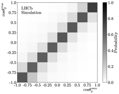
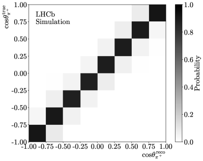
Figure 19: The detector-response matrix for the cosine of the (left) proton and (right) ${{\pi}^{+}}$ helicity angles, $\cos\theta_{p}$ and $\cos\theta_{{\pi}^{+}}$, respectively. The shading represents the interval-to-interval migration probabilities ranging from (white) 0 to (black) 1. The reconstructed values are obtained with the decay chain vertex fit.

Appendix C Four-track reconstruction efficiency

Figure 20 compares, for different track categories of the $\mathchar 28931\relax$ final-state particles, the fraction of ${{\mathchar 28931\relax}^{0}_{b}}\rightarrow{{J\mskip-3.0mu/\mskip-2.0mu\psi}}{\mathchar 28931\relax}$ signal decays that are reconstructible and four-track reconstruction efficiency as a function of the $\mathchar 28931\relax$ decay vertex position along the $z$ axis. Integrating over $z$ in the different track-type regions, the reconstructible fractions (four-track reconstruction efficiencies) amount to about 11%, 34% and 55% (72%, 55% and 60%) in the Long, Downstream and T regions, respectively. Figure 21 compares the product of the reconstructible fraction and the four-track reconstruction efficiency as a function of the $\mathchar 28931\relax$ decay vertex $z$ position to the generated distribution. The different regions account for about 17%, 40% and 43% of all the reconstructible and reconstructed events, to be compared to 40%, 37% and 23% of the generated events.

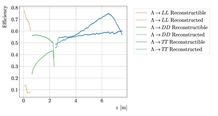
Figure 20: Fraction of ${{\mathchar 28931\relax}^{0}_{b}}\rightarrow{{J\mskip-3.0mu/\mskip-2.0mu\psi}}{\mathchar 28931\relax}$ signal decays that are reconstructible and four-track reconstruction efficiency as a function of the $\mathchar 28931\relax$ decay vertex position along the $z$ axis for the different track categories of the final-state particles (Long, Downstream and T).

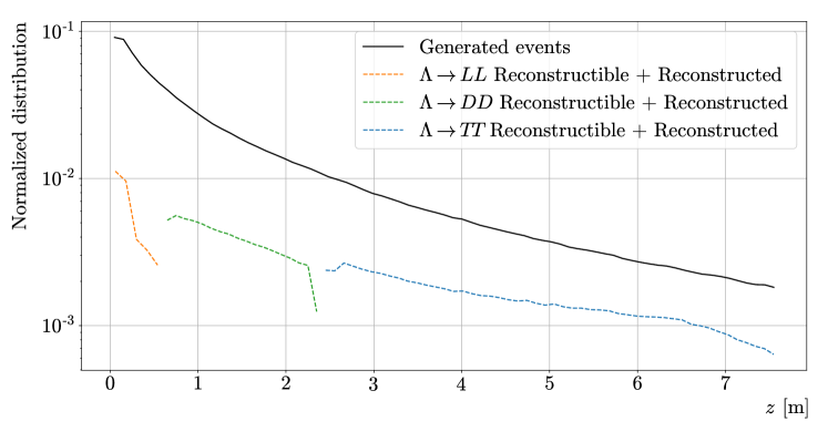
Figure 21: Fraction of ${{\mathchar 28931\relax}^{0}_{b}}\rightarrow{{J\mskip-3.0mu/\mskip-2.0mu\psi}}{\mathchar 28931\relax}$ signal decays that are reconstructible times the four-track reconstruction efficiency as a function of the $\mathchar 28931\relax$ decay vertex position along the $z$ axis for the different track categories of the final-state particles. The generated distribution is shown as a solid black line. The two distributions are normalised to the total number of generated events. The generated $\mathchar 28931\relax$ lifetime is 0.263 ns.

References

- [1] LHCb collaboration, Framework TDR for the LHCb Upgrade: Technical Design Report, CERN-LHCC-2012-007, 2012
- [2] LHCb collaboration, LHCb VELO Upgrade Technical Design Report, CERN-LHCC-2013-021, 2013
- [3] LHCb collaboration, LHCb Tracker Upgrade Technical Design Report, CERN-LHCC-2014-001, 2014
- [4] LHCb collaboration, LHCb PID Upgrade Technical Design Report, CERN-LHCC-2013-022, 2013
- [5] LHCb collaboration, LHCb Trigger and Online Upgrade Technical Design Report, CERN-LHCC-2014-016, 2014
- [6] LHCb collaboration, LHCb Upgrade Software and Computing, CERN-LHCC-2018-007, 2018
- [7] N. Cabibbo, Unitary symmetry and leptonic decays, Phys. Rev. Lett. 10 (1963) 531
- [8] M. Kobayashi and T. Maskawa, -violation in the renormalizable theory of weak interaction, Prog. Theor. Phys. 49 (1973) 652
- [9] A. Pich and E. de Rafael, Strong CP violation in an effective chiral Lagrangian approach, Nucl. Phys. B367 (1991) 313
- [10] B. Borasoy, Electric dipole moment of the neutron in chiral perturbation theory, Phys. Rev. D61 (2000)
- [11] nEDM collaboration, C. Abel et al., Measurement of the permanent electric dipole moment of the neutron, Phys. Rev. Lett. 124 (2020) 081803, arXiv:2001.11966
- [12] M. Pospelov and A. Ritz, Electric dipole moments as probes of new physics, Annals of Physics 318 (2005) 119, Special Issue
- [13] K. Jungmann, Searching for electric dipole moments, Annalen der Physik 525 (2013) 550
- [14] L. Schachinger et al., A precise measurement of the magnetic moment, Phys. Rev. Lett. 41 (1978) 1348
- [15] L. Pondrom et al., New limit on the electric dipole moment of the hyperon, Phys. Rev. D23 (1981) 814
- [16] BESIII collaboration, M. Ablikim et al., Polarization and entanglement in baryon-antibaryon pair production in electron-positron annihilation, Nature Phys. 15 (2019) 631, arXiv:1808.08917
- [17] F. J. Botella et al., On the search for the electric dipole moment of strange and charm baryons at LHC, Eur. Phys. J. C77 (2017) 181, arXiv:1612.06769
- [18] LHCb collaboration, R. Aaij et al., Measurements of the decay amplitudes and the polarisation in collisions at 7 TeV, Phys. Lett. B724 (2013) 27, arXiv:1302.5578
- [19] LHCb collaboration, R. Aaij et al., Measurement of the angular distribution and the polarisation in collisions, JHEP 06 (2020) 110, arXiv:2004.10563
- [20] ATLAS collaboration, G. Aad et al., Measurement of the parity-violating asymmetry parameter and the helicity amplitudes for the decay with the ATLAS detector, Phys. Rev. D89 (2014) 092009, arXiv:1404.1071
- [21] CMS collaboration, A. M. Sirunyan et al., Measurement of the polarization and angular parameters in decays from pp collisions at 7 and 8 TeV, Phys. Rev. D97 (2018) 072010, arXiv:1802.04867
- [22] S. P. Martin, A Supersymmetry primer, doi: 10.1142/9789812839657_0001, 10.1142/9789814307505_0001 arXiv:hep-ph/9709356, [Adv. Ser. Direct. High Energy Phys.18,1(1998)]
- [23] M. Kawasaki, K. Kohri, and T. Moroi, Big-Bang nucleosynthesis and hadronic decay of long-lived massive particles, Phys. Rev. D71 (2005) 083502, arXiv:astro-ph/0408426
- [24] K. Jedamzik, Big bang nucleosynthesis constraints on hadronically and electromagnetically decaying relic neutral particles, Phys. Rev. D74 (2006) 103509, arXiv:hep-ph/0604251
- [25] J. Alimena et al., Searching for long-lived particles beyond the Standard Model at the Large Hadron Collider, J. Phys. G47 (2020) 090501, arXiv:1903.04497
- [26] ATLAS collaboration, M. Aaboud et al., Search for long-lived charginos based on a disappearing-track signature in pp collisions at TeV with the ATLAS detector, JHEP 06 (2018) 022, arXiv:1712.02118
- [27] CMS collaboration, A. M. Sirunyan et al., Search for disappearing tracks as a signature of new long-lived particles in proton-proton collisions at 13 TeV, JHEP 08 (2018) 016, arXiv:1804.07321
- [28] ATLAS collaboration, G. Aad et al., Search for massive, long-lived particles using multitrack displaced vertices or displaced lepton pairs in pp collisions at = 8 TeV with the ATLAS detector, Phys. Rev. D92 (2015) 072004, arXiv:1504.05162
- [29] CMS collaboration, V. Khachatryan et al., Search for long-lived particles that decay into final states containing two electrons or two muons in proton-proton collisions at 8 TeV, Phys. Rev. D91 (2015) 052012, arXiv:1411.6977
- [30] CMS collaboration, Search for displaced leptons in the e-mu channel, CMS-PAS-EXO-16-022, CERN, Geneva, 2016
- [31] CMS collaboration, A. M. Sirunyan et al., A search for pair production of new light bosons decaying into muons in proton-proton collisions at 13 TeV, Phys. Lett. B796 (2019) 131, arXiv:1812.00380
- [32] ATLAS collaboration, M. Aaboud et al., Search for long-lived, massive particles in events with displaced vertices and missing transverse momentum in = 13 TeV collisions with the ATLAS detector, Phys. Rev. D97 (2018) 052012, arXiv:1710.04901
- [33] CMS collaboration, V. Khachatryan et al., Search for R-parity violating supersymmetry with displaced vertices in proton-proton collisions at = 8 TeV, Phys. Rev. D95 (2017) 012009, arXiv:1610.05133
- [34] CMS collaboration, A. M. Sirunyan et al., Search for new long-lived particles at 13 TeV, Phys. Lett. B780 (2018) 432, arXiv:1711.09120
- [35] CMS Collaboration, Search for heavy stable charged particles with of 2016 data, CMS-PAS-EXO-16-036, CERN, Geneva, 2016
- [36] ATLAS collaboration, G. Aad et al., Search for long-lived stopped R-hadrons decaying out-of-time with pp collisions using the ATLAS detector, Phys. Rev. D88 (2013) 112003, arXiv:1310.6584
- [37] CMS collaboration, A. M. Sirunyan et al., Search for decays of stopped exotic long-lived particles produced in proton-proton collisions at 13 TeV, JHEP 05 (2018) 127, arXiv:1801.00359
- [38] J. Beacham et al., Physics Beyond Colliders at CERN: beyond the standard model working group report, J. Phys. G47 (2020) 010501, arXiv:1901.09966
- [39] F. Bezrukov and D. Gorbunov, Light inflaton Hunter’s Guide, JHEP 05 (2010) 010, arXiv:0912.0390
- [40] F. Bezrukov and D. Gorbunov, Light inflaton after LHC8 and WMAP9 results, JHEP 07 (2013) 140, arXiv:1303.4395
- [41] LHCb collaboration, R. Aaij et al., Search for long-lived scalar particles in decays, Phys. Rev. D95 (2017) 071101, arXiv:1612.07818
- [42] LHCb collaboration, R. Aaij et al., Search for hidden-sector bosons in decays, Phys. Rev. Lett. 115 (2015) 161802, arXiv:1508.04094
- [43] LHCb collaboration, R. Aaij et al., Search for decays, Phys. Rev. Lett. 124 (2020) 041801, arXiv:1910.06926
- [44] LHCb collaboration, R. Aaij et al., Search for dark photons produced in 13 TeV collisions, Phys. Rev. Lett. 120 (2018) 061801, arXiv:1710.02867
- [45] P. Ilten et al., Proposed inclusive dark photon search at LHCb, Phys. Rev. Lett. 116 (2016) 251803, arXiv:1603.08926
- [46] P. Ilten, J. Thaler, M. Williams, and W. Xue, Dark photons from charm mesons at LHCb, Phys. Rev. D92 (2015) 115017, arXiv:1509.06765
- [47] LHCb collaboration, R. Aaij et al., Updated search for long-lived particles decaying to jet pairs, Eur. Phys. J. C77 (2017) 812, arXiv:1705.07332
- [48] L. Calefice et al., Effect of the high-level trigger for detecting long-lived particles at LHCb, Frontiers in Big Data 5 (2022)
- [49] LHCb collaboration, A. A. Alves Jr. et al., The LHCb detector at the LHC, JINST 3 (2008) S08005
- [50] LHCb collaboration, R. Aaij et al., LHCb detector performance, Int. J. Mod. Phys. A30 (2015) 1530022, arXiv:1412.6352
- [51] R. Aaij et al., Performance of the LHCb Vertex Locator, JINST 9 (2014) P09007, arXiv:1405.7808
- [52] R. Arink et al., Performance of the LHCb Outer Tracker, JINST 9 (2014) P01002, arXiv:1311.3893
- [53] F. Archilli et al., Performance of the muon identification at LHCb, JINST 8 (2013) P10020, arXiv:1306.0249
- [54] R. Aaij et al., The LHCb trigger and its performance in 2011, JINST 8 (2013) P04022, arXiv:1211.3055
- [55] LHCb collaboration, E. Rodrigues, Tracking definitions, CERN-LHCb-2007-006, 2007
- [56] D. Hutchcroft, VELO pattern recognition, CERN-LHCb-2007-013, 2007
- [57] LHCb collaboration, O. Callot, FastVelo, a fast and efficient pattern recognition package for the Velo, CERN-LHCb-PUB-2011-001, 2011
- [58] LHCb collaboration, R. Aaij et al., Measurement of the track reconstruction efficiency at LHCb, JINST 10 (2015) P02007, arXiv:1408.1251
- [59] O. Callot and S. Hansmann-Menzemer, The Forward Tracking: algorithm and performance studies, CERN-LHCb-2007-015, 2007
- [60] O. Callot, Downstream pattern recognition, CERN-LHCb-2007-026, 2007
- [61] O. Callot and M. Schiller, PatSeeding: a standalone track reconstruction algorithm, CERN-LHCb-2008-042, 2008
- [62] M. Needham and J. Van Tilburg, Performance of the track matching, CERN-LHCb-2007-020, 2007
- [63] M. Needham, Performance of the track matching, CERN-LHCb-2007-129, 2007
- [64] LHCb collaboration, A. Davis, M. De Cian, A. M. Dendek, and T. Szumlak, PatLongLivedTracking: a tracking algorithm for the reconstruction of the daughters of long-lived particles in LHCb, CERN-LHCb-PUB-2017-001, 2017
- [65] M. Vesterinen, A. Davis, and G. Krocker, Downstream tracking for the LHCb Upgrade, CERN-LHCb-PUB-2014-007, 2014
- [66] R. E. Kalman, A new approach to linear filtering and prediction problems, Transactions of the ASME–Journal of Basic Engineering 82 (1960) 35
- [67] R. Fruhwirth, Application of Kalman filtering to track and vertex fitting, Nucl. Instrum. Meth. A262 (1987) 444
- [68] J. Van Tilburg, Track simulation and reconstruction in LHCb, 2005. Ph.D. Thesis, Vrije Universiteit, Amsterdam, The Netherlands,
- [69] R. Frühwirth and A. Strandlie, Pattern recognition, tracking and vertex reconstruction in particle detectors, Particle Acceleration and Detection, Springer, 2020
- [70] E. Hairer, S. P. Nørsett, and G. Wanner, in Solving ordinary differential equations I: Nonstiff problems, ch. Runge-Kutta and extrapolation methods, 129–353, Springer, Berlin, Heidelberg, 1993
- [71] LHCb collaboration, E. Bos and E. Rodrigues, The LHCb track extrapolator tools, CERN-LHCb-2007-140, GLAS-PPE-2007-24, 2007
- [72] LHCb collaboration, E. Rodrigues and J. A. Hernando, Tracking event model, CERN-LHCb-2007-007, 2007
- [73] R. Aaij et al., Performance of the LHCb trigger and full real-time reconstruction in Run 2 of the LHC, JINST 14 (2019) P04013, arXiv:1812.10790
- [74] M. De Cian, S. Farry, P. Seyfert, and S. Stahl, Fast neural-net based fake track rejection in the LHCb reconstruction, LHCb-PUB-2017-011, 2017
- [75] T. Sjöstrand, S. Mrenna, and P. Skands, A brief introduction to PYTHIA 8.1, Comput. Phys. Commun. 178 (2008) 852, arXiv:0710.3820
- [76] LHCb collaboration, I. Belyaev et al., Handling of the generation of primary events in Gauss, the LHCb simulation framework, J. Phys. Conf. Ser. 331 (2011) 032047
- [77] D. J. Lange, The EvtGen particle decay simulation package, Nucl. Instrum. Meth. A462 (2001) 152
- [78] P. Golonka and Z. Was, PHOTOS Monte Carlo: A precision tool for QED corrections in and decays, Eur. Phys. J. C45 (2006) 97, arXiv:hep-ph/0506026
- [79] Geant4 collaboration, S. Agostinelli et al., Geant4: A simulation toolkit, Nucl. Instrum. Meth. A506 (2003) 250
- [80] LHCb collaboration, M. Clemencic et al., The LHCb simulation application, Gauss: Design, evolution and experience, J. Phys. Conf. Ser. 331 (2011) 032023
- [81] F. Pedregosa et al., Scikit-learn: Machine learning in Python, J. Machine Learning Res. 12 (2011) 2825, arXiv:1201.0490, and online at http://scikit-learn.org/stable/
- [82] W. D. Hulsbergen, Decay chain fitting with a Kalman filter, Nucl. Instrum. Meth. A552 (2005) 566, arXiv:physics/0503191
- [83] Particle Data Group, R. L. Workman et al., Review of particle physics, Prog. Theor. Exp. Phys. 2022 (2022) 083C01
- [84] T. Skwarnicki, A study of the radiative cascade transitions between the Upsilon-prime and Upsilon resonances, PhD thesis, Institute of Nuclear Physics, Krakow, 1986, DESY-F31-86-02
- [85] J. Podolanski and R. Armenteros, III. Analysis of V-events, The London, Edinburgh, and Dublin Philosophical Magazine and Journal of Science 45 (1954) 13