Sublattice-enriched tunability of bound states in second-order
topological insulators and superconductors

Abstract

Bound states at sharp corners have been widely viewed as the hallmark of two-dimensional second-order topological insulators and superconductors. In this work, we show that the existence of sublattice degrees of freedom can enrich the tunability of bound states on the boundary and hence lift the constraint on their locations. We take the Kane-Mele model with honeycomb-lattice structure to illustrate the underlying physics. With the introduction of an in-plane exchange field to the model, we find that the boundary Dirac mass induced by the exchange field has a sensitive dependence on the boundary sublattice termination. We find that the sensitive sublattice dependence can lead bound states to emerge at a specific type of boundary defects named as sublattice domain walls if the exchange field is of ferromagnetic nature, even in the absence of any sharp corner on the boundary. Remarkably, this sensitive dependence of the boundary Dirac mass on the boundary sublattice termination allows the positions of bound states to be manipulated to any place on the boundary for an appropriately-designed sample. With a further introduction of conventional s-wave superconductivity to the model, we find that, no matter whether the exchange field is ferromagnetic, antiferromagnetic, or ferrimagnetic, highly controllable Majorana zero modes can be achieved at the sublattice domain walls. Our work reshapes the understanding of boundary physics in second-order topological phases, and meanwhile opens potential avenues to realize highly controllable bound states for potential applications.

I Introduction

Since the discovery of two-dimensional (2D) topological insulators (TIs) Kane and Mele (2005a, b); Bernevig and Zhang (2006); Bernevig et al. (2006); König et al. (2007), an enduring and intensive exploration of topological phases in quantum materials as well as various classical systems has been witnessed Hasan and Kane (2010); Qi and Zhang (2011); Ozawa et al. (2019); Ma et al. (2019). A hallmark of topological phases is the existence of gapless states on the boundary enforced by the bulk topological invariant Chiu et al. (2016). Conventionally, the gapless states are known to be distributed on the boundary with the dimension lower than the bulk by one. In other words, the gapless boundary states have codimension $d_{c}=1$. Recently, it has been uncovered that there in fact exists a large class of topological phases whose gapless boundary states have $d_{c}\geq 2$ Sitte et al. (2012); Zhang et al. (2013); Benalcazar et al. (2017a, b); Schindler et al. (2018a); Song et al. (2017); Langbehn et al. (2017); Liu and Wakabayashi (2017); Ezawa (2018); Geier et al. (2018); Khalaf (2018); Yan et al. (2018); Wang et al. (2018a, b); Yan (2019a); Liu et al. (2019); Kudo et al. (2019); Chen et al. (2020a); Huang and Liu (2020); Hu et al. (2020); Zhang et al. (2021). For distinction, now a topological phase is dubbed as an $n$th-order topological phase if it only supports gapless boundary states with $d_{c}=n$ Yan (2019b); Schindler (2020); Xie et al. (2021).

Different orders of topological phases have a hierarchy connection Călugăru et al. (2019). In principle, an $n$th-order topological phase could be descended from an $(n-1)$th-order topological phase by appropriately lifting the protecting symmetry. A paradigmatic example is the realization of a second-order TI by lifting the time-reversal symmetry of a first-order TI Sitte et al. (2012); Zhang et al. (2013); Ren et al. (2020); Chen et al. (2020b); Huang et al. (2022). The physics behind such a transition can be intuitively understood via the Jackiw-Rebbi theory based on low-energy boundary Dirac-Hamiltonians Jackiw and Rebbi (1976); Yan (2019b); Schindler (2020). That is, the breaking of time-reversal symmetry, e.g., by applying a magnetic field, will introduce a boundary Dirac mass to gap out the helical boundary (surface or edge) states, leading to a trivialization of the first-order topological insulating phase Shen (2013). Interestingly, the induced Dirac mass generally shows a dependence on the orientation of the boundary and may change sign across some direction Khalaf (2018). When the Dirac masses on two boundaries with different orientations have opposites signs, a Dirac-mass domain wall harboring gapless states with $d_{c}=2$ will be formed at their intersection Jackiw and Rebbi (1976), a corner in 2D Ren et al. (2020); Chen et al. (2020b); Huang et al. (2022); Zhu (2018); Zhuang and Yan (2022), or a hinge in 3D Sitte et al. (2012); Zhang et al. (2013, 2019a); Kheirkhah et al. (2021, 2022a). Because of the generality of this domain-wall picture, bound states positioned at corners in 2D systems Peterson et al. (2018); Serra-Garcia et al. (2018); Imhof et al. (2018); Zhang et al. (2019b); Chen et al. (2019); Fan et al. (2019); El Hassan et al. (2019) and chiral or helical states propagating along hinges in 3D systems Schindler et al. (2018b); Gray et al. (2019); Choi et al. (2020); Noguchi et al. (2021); Aggarwal et al. (2021); Shumiya et al. (2022) have been widely taken as the defining boundary characteristic of second-order topology.

When the sign of the boundary Dirac mass for a given system is only sensitive to the orientation of the boundary, e.g., a higher-order topological phase enforced by mirror symmetry Langbehn et al. (2017); Geier et al. (2018), it is true that the bound states will be strongly bounded at sharp corners or hinges where the orientation of the boundary has a dramatic change. However, if the boundary Dirac mass is also sensitive to other factors on the boundary, then it is possible that the bound states are not necessarily pinned at sharp corners or hinges, but instead are allowed to be positioned anywhere on the boundary. Obviously, the tunability of bound states could make the observation of many interesting phenomena possible, such as the creation of additional bound states or the annihilation of bound states. Recently, we did find that the sign of boundary Dirac mass in systems with sublattice degrees of freedom can have a sensitive dependence on the boundary sublattice termination in the context of second-order topological superconductors (TSCs) Zhu et al. (2022); Kheirkhah et al. (2022b). Concretely, we found that when a 2D first-order TI with honeycomb Zhu et al. (2022) or kagome lattice structure Kheirkhah et al. (2022b) is placed on an unconventional superconductor, e.g., a d-wave superconductor, the Dirac mass induced by superconductivity gapping out the helical edge states exhibits a sensitive dependence on the type of terminating sublattices on the boundary. This property allows the realization of Majorana Kramers pairs (a Majorana Kramers pair corresponds to two Majorana zero modes (MZMs) related by time-reversal symmetry Haim and Oreg (2019)) at the so-called sublattice domain walls, a type of boundary defects corresponding to the intersection of two edges with the same orientation but with different sublattice terminations, see illustration in Fig.1. Remarkably, the Majorana Kramers pairs with $d_{c}=2$ can emerge even without the existence of sharp corners (e.g., a cylindrical geometry with one direction being periodic) Zhu et al. (2022), and their positions can be manipulated by tuning the sublattice terminations Zhu et al. (2022); Kheirkhah et al. (2022b), which may benefit the future application of Majorana bound states in topological quantum computation Nayak et al. (2008); Liu et al. (2014); Gao et al. (2016); Schrade and Fu (2018).

It is known that when the time-reversal symmetry is broken, the helical boundary states of a first-order TI would be gapped out Yu et al. (2010); Qi and Zhang (2011). The time-reversal symmetry could be broken by an exchange field, which itself could be induced by an emergent intrinsic magnetic order or magnetic proximity effect from a substrate magnetic insulator. As Dirac domain walls can exist in both superconductors and insulators, it is natural to expect that the Dirac mass induced by exchange field may also have similar sensitive dependence on the sublattice termination, and the realization of bound states at sublattice domain walls may also occur in the context of second-order TIs. In this work, we take the paradigmatic Kane-Mele model with honeycomb lattice structure to demonstrate this expectation Kane and Mele (2005a, b). The Kane-Mele model is known to support first-order topological insulating phase, and the honeycomb lattice contains only two sublattice degrees of freedom (labeled as A and B for discussion). Following previous works, we consider that the exchange field lies in the lattice plane Ren et al. (2020); Chen et al. (2020b), and for generality we consider that the collinear magnetic moments on the two types of sublattices satisfy $\boldsymbol{M}_{A}=\gamma\boldsymbol{M}_{B}$ with $-1\leq\gamma\leq 1$. Correspondingly, $0\leq\gamma\leq 1$ refers to a ferromagnetic order, $\gamma=-1$ refers to an antiferromagnetic order, and $-1<\gamma<0$ refers to a ferrimagntic order. Based on the low-energy edge theory Yan et al. (2018); Zhu et al. (2022), we determine the boundary Dirac masses on the two types of edges whose terminations contain only one type of sublattices (commonly dubbed zigzag and beard edges Castro Neto et al. (2009)).

Our main findings can be briefly summarized as follows. First, we find that, for the zigzag and beard edges with the same orientation, whether the values or signs of the Dirac masses on them are the same or not depends on the value of $\gamma$. Somewhat counterintuitively, we find that, for an antiferromagnetic or ferrimagnetic exchange field, i.e., $-1\leq\gamma<0$, the Dirac masses on them take the same sign, even though the directions of the exchange field are opposite on the outermost terminating sublattices for these two kinds of edges, as depicted in Fig.1(a). On the contrary, for a ferromagnetic exchange field, we find that the Dirac masses on them take opposite signs, even though the directions of the exchange field are the same on the outermost terminating sublattices for these two kinds of edges, as depicted in Fig.1(b). Because of the sign difference in Dirac masses, we find that the ferromagnetic exchange field can induce highly controllable bound states at the sublattice domain walls corresponding to the intersection of zigzag and beard edges. As an important consequence, bound states can be achieved even in the absence of any sharp corner on the boundary. As the boundary Dirac mass induced by exchange field and the effective chemical potential on the boundary turn out to have a sensitive dependence on the sublattice terminations, we show that these properties allows the realization of MZMs at the sublattice domain walls even one considers conventional s-wave superconductivity which, in the absence of exchange field, will introduce a uniform boundary Dirac mass Zhu et al. (2022). Our findings suggest that the ubiquitous sublattice degrees of freedom in materials provide a knob to control and manipulate the positions of bound states in second-order topological phases.

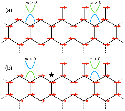
Figure 1: (Color online) A schematic diagram of the sublattice domain walls and the dependence of boundary Dirac mass ($m$) on the sublattice termination. The upper boundary consists of two parts, with one part being a zigzag edge (top left hand side in each panel) and the other being a beard edge (top right hand side in each panel), leading to the formation of sublattice domain walls at their intersections. The blue and green parabolas represent massive Dirac energy spectra of the gapped edge states. Different color patterns are just used to intuitively illustrate whether the signs of Dirac masses on the two sides of the sublattice domain wall are the same [(a)] or opposite [(b)]. On each site, the red arrow denotes the direction of the exchange field. (a) When the exchange field is antiferromagnetic, the boundary Dirac masses on the upper zigzag and beard edges have the same sign, accordingly, the sublattice domain wall is not a Dirac-mass domain wall and hence does not harbor any bound states. (b) When the exchange field is ferromagnetic, the boundary Dirac masses on the upper zigzag and beard edges have opposite signs, hence the sublattice domain wall is a Dirac-mass domain wall supporting bound state illustrated by the black star.

This paper is organized as follows. In Sec.II, we introduce the Hamiltonian describing a first-order TI subjected to an in-plane exchange field. In Sec.III, we establish a theory distinct from the one developed by Ren et al. Ren et al. (2020) to understand the robustness of helical edge states on the armchair edges, and show that the helical edge states on the armchair edges will be gapped out once the exchange fields on the two sublattices are different, leading to the presence of corner bound states in samples with geometries different from the one with diamond shape considered in Ref. Ren et al. (2020). In Sec.IV, we derive the low-energy boundary Hamiltonians on the beard and zigzag edges, and show explicitly the dependence of boundary Dirac masses on the sublattice terminations. The presence of bound states at the sublattice domain walls is also numerically demonstrated. In Sec.V, we further consider the introduction of s-wave superconductivity to the system and show the presence of MZMs at the sublattice domain walls. We discuss the results and conclude the paper in Sec.VI. Some calculating details of the low-energy boundary Hamiltonians are relegated to appendices.

II Kane-Mele model with an in-plane exchange field

We start with the Hamiltonian Kane and Mele (2005a, b)

$$H = t\sum_{\langle ij\rangle,\alpha}c_{i,\alpha}^{{\dagger}}c_{j,\alpha}+i\lambda_{\rm so}\sum_{\langle\langle ij\rangle\rangle,\alpha,\beta}\nu_{ij}c_{i,\alpha}^{{\dagger}}(s_{z})_{\alpha\beta}c_{j,\beta}$$ (1)

$$+\lambda_{\nu}\sum_{i,\alpha}\xi_{i}c_{i,\alpha}^{{\dagger}}c_{i,\alpha}+\sum_{i,\alpha,\beta}c_{i,\alpha}^{{\dagger}}(\boldsymbol{M}_{i}\cdot\mathbf{s})_{\alpha\beta}c_{i,\beta},$$

where $c_{i,\alpha}^{{\dagger}}$ $(c_{i,\alpha})$ refers to a fermion creation (annihilation) operator at site $i$, the subscripts $\alpha$ and $\beta$ refer to spin indices, $t$ denotes the hopping energy, $\lambda_{\rm so}$ characterizes the strength of intrinsic spin-orbit coupling, $\nu_{ij}=1(-1)$ for a clockwise (anticlockwise) path along which the electrons hop from site $j$ to site $i$, $\lambda_{\nu}$ characterizes the staggered sublattice potential ($\xi_{i}=\pm 1$), and the last term describes the exchange field induced by certain collinear magnetic order (the involving $g$-factor and $\hbar$ are made implicity for notational simplicity). The notations $\langle ij\rangle$ and $\langle\langle ij\rangle\rangle$ mean that the sum is over nearest-neighbor sites and next-nearest-neighbor sites, respectively. As in this paper we are interested in second-order topology, the collinear magnetic order will be assumed to lie in the lattice plane, i.e., $\boldsymbol{M}_{i\in A}=\boldsymbol{M}=(M_{x},M_{y},0)$, and for generality we consider $\boldsymbol{M}_{i\in B}=\gamma\boldsymbol{M}$ with $-1\leq\gamma\leq 1$ to take all possible in-plane collinear magnetic orders into account.

By performing a Fourier transformation and choosing the basis to be $\psi_{k}=(c_{k,A,\uparrow},c_{k,B,\uparrow},c_{k,A,\downarrow},c_{k,B,\downarrow})^{T}$, the Hamiltonian in momentum space reads

$$\mathcal{H}(\boldsymbol{k}) = t\sum_{i=1}^{3}[\cos(\boldsymbol{k}\cdot\boldsymbol{a}_{i})s_{0}\sigma_{x}+\sin(\boldsymbol{k}\cdot\boldsymbol{a}_{i})s_{0}\sigma_{y}]$$ (2)

$$+2\lambda_{\rm so}\sum_{i=1}^{3}\sin(\boldsymbol{k}\cdot\boldsymbol{b}_{i})s_{z}\sigma_{z}+\lambda_{\nu}s_{0}\sigma_{z}$$

$$+\frac{1+\gamma}{2}(\boldsymbol{M}\cdot\mathbf{s})\sigma_{0}+\frac{1-\gamma}{2}(\boldsymbol{M}\cdot\mathbf{s})\sigma_{z},$$

where the Pauli matrices $s_{i}$ and $\sigma_{i}$, and the identity matrices $s_{0}$ and $\sigma_{0}$, act on the spin ($\uparrow,\downarrow$) and sublattice (A,B) degrees of freedom, respectively. $\boldsymbol{a}_{i}$ refers to the nearest-neighbor vectors, with $\boldsymbol{a}_{1}=a(0,1)$, $\boldsymbol{a}_{2}=\frac{a}{2}(\sqrt{3},-1)$, $\boldsymbol{a}_{3}=\frac{a}{2}(-\sqrt{3},-1)$ (throughout the paper we set the lattice constant $a=1$ for notational simplicity). The next-nearest-neighbor vectors $\boldsymbol{b}_{1}=\boldsymbol{a}_{2}-\boldsymbol{a}_{3}$, $\boldsymbol{b}_{2}=\boldsymbol{a}_{3}-\boldsymbol{a}_{1}$ and $\boldsymbol{b}_{3}=\boldsymbol{a}_{1}-\boldsymbol{a}_{2}$ Haldane (1988). The last line in (2) means that a general collinear exchange field can be decomposed as the sum of a uniform ferromagnetic exchange field and an antiferromagnetic one. Without the two time-reversal-symmetry-breaking terms in the last line, the Hamiltonian describes a first-order TI when $|\lambda_{\nu}|<3\sqrt{3}|\lambda_{\rm so}|$ Kane and Mele (2005b).

III Helical edge states and corner bound states on the boundary

Considering the Kane-Mele model with only the ferromagnetic term, Ren et al. showed that the helical edge states would be gapped out on the zigzag edges, but remain gapless on the armchair edges Ren et al. (2020), irrespective of the direction of the in-plane ferromagnetic exchange field. In order to avoid gapless edge states with codimension $d_{c}=1$ and only have bound states with $d_{c}=2$ on the boundary, Ren et al. suggested a diamond-shaped nanoflake with only zigzag boundaries. For such a geometry, they showed that helical edge states are gapped out on all edges, while bound states show up at half of the corners Ren et al. (2020). By a close look of the Fig.1 therein, one can notice that these corners hosting bound states correspond to the intersections of two adjacent zigzag edges with different orientations as well as distinct sublattice terminations.

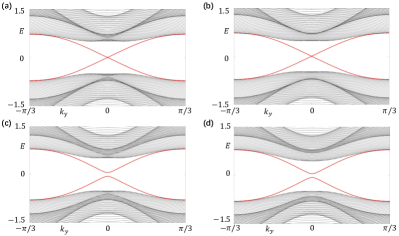
Figure 2: (Color online) Energy spectra for a ribbon with armchair edges. The ribbon has open boundary conditions in the $x$ direction and periodic boundary conditions in the $y$ direction. Chosen parameters are $t=1$, $\lambda_{\rm so}=0.1$, $M_{x}=M_{y}=0.2$. (a) $\lambda_{\nu}=0$, $\gamma=1$, (b) $\lambda_{\nu}=0.1$, $\gamma=1$, (c) $\lambda_{\nu}=0$, $\gamma=0.5$, (d) $\lambda_{\nu}=0.1$, $\gamma=0.5$.

In Ref. Ren et al. (2020), the reason that the helical edge states are stable against the in-plane exchange field (corresponding to $\gamma=1$) was attributed to the existence of an additional mirror symmetry on the armchair edges, which provides a further protection. In more detail, it is known that $k_{y}$ remains a good quantum number on the armchair edges if periodic boundary conditions are imposed in the $y$ direction. In Ref. Ren et al. (2020), the authors considered the limit without the staggered sublattice potential, i.e., $\lambda_{\nu}=0$, and found that the reduced Hamiltonian $\mathcal{H}(k_{x},k_{y}=0)$ has a mirror symmetry, with the symmetry operator taking the general form $\mathcal{M}_{n}=i(\hat{\boldsymbol{n}}\cdot\mathbf{s})\sigma_{x}$, where $\hat{\boldsymbol{n}}$ denotes the direction of the magnetic moment. As $[\mathcal{H}(k_{x},0),\mathcal{M}_{n}]=0$, $\mathcal{H}(k_{x},0)$ can be decomposed as a direct sum of two sectors for any $k_{x}$ according to the two eigenvalues ($\pm i$) of the mirror operator, and it turns out that the two sectors carry opposite winding numbers, $\omega^{\pm i}=\pm 1$. Although this explanation is valid in the limit with $\lambda_{\nu}=0$, it is in fact not essential. To see this, we would like to point out that the helical edge states in fact remain gapless when $\lambda_{\nu}\neq 0$, as long as the exchange field has the same value on the two types of sublattices, i.e., $\gamma=1$, as shown in Figs.2(a)(b). However, once $\lambda_{\nu}\neq 0$, the aforementioned mirror symmetry is explicitly broken by the staggered sublattice potential (note $[\lambda_{\nu}s_{0}\sigma_{z},\mathcal{M}_{n}]\neq 0$). Accordingly, the Hamiltonian can no longer be decomposed into two mirror sectors, and the topological analysis based on the mirror-graded winding numbers in Ref. Ren et al. (2020) breaks down. Nevertheless, the robustness of the crossing at $k_{y}=0$ on the armchair edges even when $\lambda_{\nu}\neq 0$ suggests the existence of a topological protection. Viewing $\mathcal{H}(k_{x},0)$ as a one-dimensional Hamiltonian, the double degeneracy of the crossing on one armchair edge suggests the existence of two zero-energy bound states at each end of the one-dimensional system. As the spinful time-reversal symmetry is explicitly broken by the exchange field, it is known that in one dimension only chiral symmetry can protect the existence of two degenerate bound states at the same end Schnyder et al. (2008); Kitaev (2009). We find that the chiral symmetry operator for the one-dimensional Hamiltonian $\mathcal{H}(k_{x},0)$ has the form $\mathcal{C}=s_{z}\sigma_{y}$. Accordingly, one can define a winding number to characterize the full Hamiltonian $\mathcal{H}(k_{x},0)$. The winding number is given by Ryu et al. (2010)

$$\omega=\frac{1}{2\pi i}\int_{BZ}dk_{x}\text{Tr}[Q^{-1}(k_{x})\partial_{k_{x}}Q(k_{x})],$$ (3)

where “BZ” stands for Brillouin zone, “Tr” stands for the trace operation, and $Q(k_{x})$ is related to the Hamiltonian and determined by rewriting the Hamiltonian into a new basis under which the chiral symmetry operator is diagonal, i.e., $\mathcal{\tilde{C}}=diag\{1,1,-1,-1\}$, correspondingly,

$$\tilde{\mathcal{H}}(k_{x},0)=\left(\begin{array}[]{cc}0&Q(k_{x})\\ Q^{{\dagger}}(k_{x})&0\\ \end{array}\right).$$ (6)

Here the explicit form of $Q(k_{x})$ is

$$Q(k_{x})=\left(\begin{array}[]{cc}M_{x}-iM_{y}&F(k_{x})-i\lambda_{\nu}\\ F(k_{x})+i\lambda_{\nu}&M_{x}+iM_{y}\\ \end{array}\right),$$ (9)

where $F(k_{x})=t[2\cos(\frac{\sqrt{3}}{2}k_{x})+1]-i2\lambda_{\rm so}[\sin(\sqrt{3}k_{x})-2\sin(\frac{\sqrt{3}}{2}k_{x})]$. Since the chiral symmetry is preserved even when $\lambda_{\nu}$, $M_{x}$ and $M_{y}$ are all nonzero, the topological invariant will hold its value as long as the bulk energy gap of $\mathcal{H}(k_{x},0)$ remains open, therefore, the winding number can be determined by considering the limit with $\lambda_{\nu}=M_{x}=M_{y}=0$. Accordingly, it is easy to find that

$$\omega=\frac{1}{2\pi i}\int_{BZ}dk_{x}2F^{-1}(k_{x})\partial_{k_{x}}F(k_{x})=2.$$ (10)

The chiral symmetry and the value of the winding number explain the robustness of the doubly-degenerate crossing of the helical edge states on the armchair edges even when $\lambda_{\nu}\neq 0$.

Figure 3: (Color online) Corner bound states in a rectangular sample with both $x$ and $y$ directions taking open boundary conditions. Chosen parameters are $t=1$, $\lambda_{\rm so}=0.1$, $M_{x}=M_{y}=0.2$, $\gamma=0.3$, $\lambda_{\nu}=0$ and $N_{x}=N_{y}=28$. The geometries of the samples are depicted in (a2) and (b2), and a few corresponding eigenenergies near zero energy are shown in (a1) and (b1). The red dots in (a1) and (b1) correspond to the eigenergies of the corner bound states. The shade of the red color on the lattice sites in (a2) and (b2) reflects the weight of the probability density of the corner bound states.

When $\gamma\neq 1$, it is easy to find that the antiferromagnetic term in Hamiltonian (2) commutes with the chiral symmetry operator, i.e., $[(\boldsymbol{M}\cdot\mathbf{s})\sigma_{z},\mathcal{C}]=0$, indicating that the antiferromagnetic term breaks the chiral symmetry of $\mathcal{H}(k_{x},0)$. As a result, the protection of the crossing at $k_{y}=0$ from the chiral symmetry is lifted and the helical edge states on the armchair edges would be gapped out by the antiferromagnetic term. As shown in Figs.2(c)(d), the numerical results confirm this expectation, reflecting the correctness of our analysis.

The opening of an energy gap to the helical edge states on the armchair edges implies an important consequence: one no longer needs to avoid the armchair edges to achieve corner bound states. Now bound states are also possible to emerge at the corners corresponding to the intersections of armchair edges and other types of edges, such as zigzag or beard edges. By numerical calculations, we confirm this expectation, as shown in Fig.3. According to the numerical results shown in Figs.3(a1)(a2), one can see that the two bound states are localized around the two bottom corners for a rectangular sample with armchair edges in the $x$ direction and beard edges in the $y$ direction. Interestingly, when the beard edges are modified to zigzag edges by changing only the outermost sublattices of the $y$-normal edges, the positions of the two bound states are found to shift dramatically to the two top corners, as illustrated in Figs.3(b1)(b2). We will adopt the edge theory to show in the next section that this is because the boundary Dirac mass has a sensitive dependence on the boundary sublattice termination, and can switch its sign when the boundary sublattice termination is changed from one type to the other.

It is worth pointing out that here the antiferromagnetic or ferrimagnetic exchange field does not favor the realization of corner bound states. This can be proved by numerical calculations or simply inferred by noting that in the limit $\lambda_{\nu}=0$ and $\gamma=-1$, the momentum-independent antiferromagnetic exchange field anticommutes with all other terms in the Hamiltonian (2). Since this implies that the antiferromagnetic term will introduce a constant gap to the energy spectrum which cannot be closed by tuning the parameters of all other terms, the resulting gapped phase is topologically connected to an atomic trivial insulator without any types of topological mid-gap states on the boundary.

IV Bound states at sublattice domain walls

In the following, we are going to show that bound states can also be achieved even without the existence of sharp corners, and their locations can be freely tuned by taking advantage of the sublattice degrees of freedom. In a previous work, we have revealed that for the Kane-Mele model, the boundary sublattice terminations have a strong impact on the helical edge states, such as the shift of the boundary Dirac points (the crossing point of the energy spectra for helical edge states) from one time-reversal invariant momentum to the other in the boundary Brillouin zone Zhu et al. (2022). In addition, the sublattice terminations can also strongly affect the boundary Dirac mass induced by superconductivity and hence the formation of Dirac-mass domain walls supporting Majorana Kramers pairs Zhu et al. (2022).

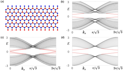
Figure 4: (Color online) Energy spectra for a ribbon with periodic boundary conditions in the $x$ direction and beard edges in the $y$ direction. Chosen parameters are $t=1$, $\lambda_{\rm so}=0.1$, $M_{x}=M_{y}=0.2$, $\lambda_{\nu}=0$ and $N_{y}=100$. (a) A schematic diagram of a sample with beard edges in the $y$ direction. Blue and red sites correspond to A-type and B-type sublattices, respectively. The red solid lines in (b-d) denote energy spectra of the edge states on the beard edges. (b) $\gamma=1$, the helical edge states on the upper and lower beard edges are gapped out. (c) $\gamma=0$, the helical edge states on the upper beard edge are gapped out, while the helical edge states on the lower beard edge remain almost gapless. (d) $\gamma=-1$, the helical edge states on the upper and lower beard edges are gapped out.

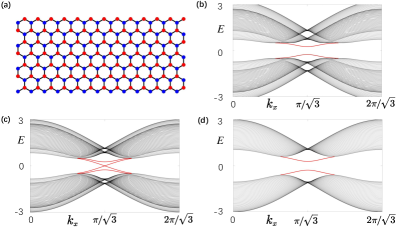
Figure 5: (Color online) Energy spectra for a ribbon with periodic boundary conditions in the $x$ direction and zigzag edges in the $y$ direction. Chosen parameters are $t=1$, $\lambda_{\rm so}=0.1$, $M_{x}=M_{y}=0.2$, $\lambda_{\nu}=0$ and $N_{y}=100$. (a) A schematic diagram of a sample with zigzag edges in the $y$ direction. The red solid lines in (b-d) denote energy spectra of the edge states on the zigzag edges. (b) $\gamma=1$, the helical edge states on the upper and lower zigzag edges are gapped out. (c) $\gamma=0$, the helical edge states on the upper zigzag edge remain almost gapless, while the helical edge states on the lower zigzag edge are gapped out. (d) $\gamma=-1$, the helical edge states on the upper and lower zigzag edges are gapped out.

To explore the impact of sublattice terminations on the boundary Dirac mass induced by exchange field, we first numerically calculate the energy spectra for a ribbon with the $x$ direction taking periodic boundary conditions and the $y$ direction having only beard or zigzag edges, as illustrated in Figs.4(a) and 5(a). According to the results presented in Figs.4(b-d) and 5(b-d), one can infer that the boundary energy spectra (red solid lines) for the upper and lower beard or zigzag edges are degenerate when $\gamma=\pm 1$, suggesting that the Dirac masses induced by the exchange field on the upper and lower beard or zigzag edges have the same magnitude for these two limiting cases. On the other hand, the results for $\gamma=0$ clearly reveal that the boundary Dirac mass strongly depends on the sublattice termination for a given boundary. To be specific, let us focus on the upper $y$-normal boundary for a more detailed discussion. When $\gamma=0$, based on the edges at which the mid-gap states are localized, we find that the Dirac mass is vanishingly small when the upper $y$-normal boundary terminates with B sublattices, as illustrated in Fig.5(c). Obviously, the smallness of the Dirac mass should be related to the fact that exchange fields on B sublattices are absent when $\gamma=0$. This implies that, for a given sublattice termination, the magnitude of the exchange field on the corresponding sublattices determines the main contribution to the magnitude of the Dirac mass.

As it turns out that both ferromagnetic and antiferromagnetic exchange fields can induce a finite Dirac mass to the helical edge states, regardless of the boundary sublattice terminations, a natural question to ask is: for a given type of exchange field, do the boundary Dirac masses associated with the two kinds of sublattice terminations have the same sign or opposite signs? Naively, one may think that when $\gamma>0$, since the exchange fields take the same direction on the two types of sublattices, the Dirac masses should also take the same sign for the two kinds of sublattice terminations. In contrast, when $\gamma<0$, since the exchange fields take opposite directions on the two kinds of sublattices, one may think that the Dirac masses associated with the two kinds of sublattice terminations should also take opposite signs. However, we find that the results are just the opposite. To show this, we focus on the upper $y$-normal boundary and derive the low-energy Hamiltonians describing the boundary physics on the zigzag and beard edges.

Here we focus on the limit $\lambda_{\nu}=0$ and consider $t$ and $\lambda_{\rm so}$ to be positive constants for the convenience of discussion. First, let us consider the upper $y$-normal boundary to be a beard edge (terminating with A sublattices, see the upper edge in Fig.4(a)). We find that the corresponding low-energy Hamiltonian has the form (see details in Appendix A)

$$\mathcal{H}_{b}(q_{x})=vq_{x}s_{z}+M_{x}s_{x}+M_{y}s_{y},$$ (11)

where $q_{x}$ denotes a small momentum measured from $k_{x}=0$ at which the boundary Dirac point is located (see the dispersion of edge states in Fig.4), and the velocity of the helical edge states is $v=3\sqrt{3}\lambda_{\rm so}$. On the other hand, when the upper $y$-normal boundary is a zigzag edge (terminating with B sublattices, see the upper edge Fig.5(a)), we find that the low-energy Hamiltonian has the form (see details in Appendix B)

$$\mathcal{H}_{z}(q_{x}^{\prime})=v^{\prime}q_{x}^{\prime}s_{z}+\frac{1-\gamma\eta^{2}}{1+\eta^{2}}(M_{x}s_{x}+M_{y}s_{y}),$$ (12)

where $q_{x}^{\prime}$ denotes the momentum measured from $k_{x}=\pi/\sqrt{3}$ at which the boundary Dirac point is located (see Fig.5(c)), and the explicit expressions of the parameters read

$$v^{\prime} = \frac{2\sqrt{3}t\lambda_{\rm so}\eta}{1+\eta^{2}}+\frac{2\sqrt{3}\lambda_{\rm so}(\eta^{2}-1)}{1+\eta^{2}},$$

$$\eta = \frac{4t\lambda_{\rm so}}{\sqrt{t^{2}(t^{2}+16\lambda_{\rm so}^{2})}-t^{2}}.$$ (13)

In real materials, $\lambda_{\rm so}$ is commonly much smaller than $t$. Focusing on the regime $\lambda_{\rm so}\ll t$, it is easy to find that $\eta\simeq t/2\lambda_{\rm so}\gg 1$, and the Hamiltonian can be approximately reduced as

$$\mathcal{H}_{z}(q_{x}^{\prime})\approx 2vq_{x}^{\prime}s_{z}-\gamma(M_{x}s_{x}+M_{y}s_{y}).$$ (14)

The two low-energy Hamiltonians, (11) and (12), provide a clear understanding of the dependence of the boundary Dirac mass on the exchange field and sublattice termination. Remarkably, the results show that the Dirac masses on the zigzag and beard edges with the same orientation have opposite signs when $\gamma>\gamma_{c}=\eta^{-2}$, and the same sign when $\gamma<\gamma_{c}$. When $\eta\gg 1$, the critical value $\gamma_{c}$ can be set as zero.

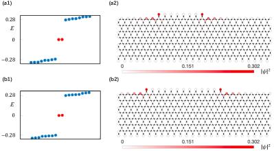
Figure 6: (Color online) Tunable bound states at the sublattice domain walls. Chosen parameters are $t=1$, $\lambda_{\rm so}=0.1$, $M_{x}=M_{y}=0.2$, $\gamma=1$ and $\lambda_{\nu}=0$. (a1) and (b1) show the energy spectra (only a few eigenenergies near zero energy are shown) corresponding to systems with the geometries shown in (a2) and (b2), respectively. Periodic boundary conditions are imposed in the $x$ direction, namely, the left and right armchair edges in (a2) and (b2) are connected when diagonalizing the Hamiltonian. The red dots in (a1) and (b1) correspond to the eigenenergies of the bound states at the sublattice domain walls. The shade of the red color on the lattice sites in (a2) and (b2) reflects the weight of the probability density of the bound states.

As Dirac masses of opposite signs lead to the formation of domain walls hosting bound states Jackiw and Rebbi (1976), apparently, the dependence of Dirac mass on the sublattice termination shown in the two low-energy boundary Hamiltonians suggests that Dirac-mass domain walls can form on the same $y$-normal boundary. Put it more explicitly, when $\gamma>\gamma_{c}$ and the $y$-normal boundary consists of two flat parts, with one part taking the beard edge (terminating with A sublattices) and the other taking the zigzag edge (terminating with B sublattices), then the sublattice domain walls, which correspond to the intersections of the beard and zigzag edges, are Dirac-mass domain walls hosting bound states. The numerical results shown in Fig.6 confirm this expectation. We would like to emphasize two important properties of the sublattice domain walls that can be inferred from the numerical results. First, as the sublattice domain walls on the same boundary can support bound states, it suggests that sharp corners are not a necessary condition to achieve bound states in a second-order topological phase if the boundary Dirac mass shows sensitive dependence on the sublattice terminations. Indeed, Fig.6 demonstrates that bound states are present even though there is no sharp corner in the system with periodic boundary conditions in one direction. Second, as the bound states are associated with the sublattice domain walls, it suggests that the locations of the bound states can be tuned by locally manipulating the sublattice termination. This fact can be intuitively inferred by a comparison of the locations of the bound states in Figs.6(a2)(b2).

In addition to the exchange field, it is known that the superconductivity can also induce a Dirac mass to the helical edge states and gap them out Fu and Kane (2009). An important fact to note is that the Dirac masses induced by exchange field and superconductivity are competing in nature. Above we have shown that the Dirac masses induced by exchange field on the two sides of a sublattice domain wall can have different magnitude and signs. Apparently, this raises the possibility to realize domain walls with the Dirac mass on one side dominated by the superconductivity and on the other side dominated by the exchange field. It is known that MZMs will emerge at such domain walls Fu and Kane (2009); Yan (2019c); Jäck et al. (2019); Wu et al. (2020a). In the following, we consider conventional s-wave superconductivity to demonstrate that MZMs can be realized at the sublattice domain walls.

V Majorana zero modes at sublattice domain walls

Before proceeding, it is worth pointing out that a number of proposals on the realization of 2D second-order TSCs or topological superfluids have been raised in the past few years, including TI/superconductor heterostructures Yan et al. (2018); Wang et al. (2018a); Liu et al. (2018); Zhang et al. (2019c); Pan et al. (2019); Wu et al. (2020a); Kheirkhah et al. (2020a); Laubscher et al. (2020); Li and Yan (2021); Li and Zhou (2021); Tan et al. (2022); Wu et al. (2022), superconductors with mixed-parity pairings Wang et al. (2018b); Wu et al. (2019a); Ikegaya et al. (2021); Roy (2020), spin-orbit coupled superconductors with s+id pairing Zhu (2019); Kheirkhah et al. (2020b), odd-parity superconductors Zhu (2018); Yan (2019a); Ahn and Yang (2020); Hsu et al. (2020); Li et al. (2021); Scammell et al. (2022), etc Zeng et al. (2019); Volpez et al. (2019); Franca et al. (2019); Huang et al. (2019); Wu et al. (2020b, c, 2021); Qin et al. (2022); Roy and Juričić (2021), also with the MZMs localized at sharp corners being the smoking gun. Among the various proposals, the TI/superconductor heterostructures are arguably most close to implementation owing to the abundance of candidate materials.

By putting the TI described by the Kane-Mele model in proximity to an s-wave superconductor, the whole system can be effectively described by a Bogoliubov-de Gennes (BdG) Hamiltonian. Consider the basis $\Psi_{\boldsymbol{k}}=(\psi_{\boldsymbol{k}},\psi_{-\boldsymbol{k}}^{{\dagger}})^{T}$, $H=\frac{1}{2}\sum_{\boldsymbol{k}}\Psi_{\boldsymbol{k}}^{{\dagger}}\mathcal{H}_{\rm BdG}(\boldsymbol{k})\Psi_{\boldsymbol{k}}$ with

$$\mathcal{H}_{\rm BdG}(\boldsymbol{k})=\left(\begin{array}[]{cc}\mathcal{H}(\boldsymbol{k})-\mu s_{0}\sigma_{0}&i\Delta s_{y}\sigma_{0}\\ -i\Delta^{*}s_{y}\sigma_{0}&-\mathcal{H}^{*}(-\boldsymbol{k})+\mu s_{0}\sigma_{0}\\ \end{array}\right),\quad$$ (17)

where $\mu$ is the chemical potential, and $\Delta$ is the s-wave pairing amplitude. Below we will assume $\Delta$ to be a momentum-independent real constant for the convenience of discussion.

To show intuitively that MZMs can emerge at the sublattice domain walls, we derive the corresponding low-energy boundary Hamiltonian based on the BdG Hamiltonian. For generality, now we consider the staggered sublattice potential to be finite. Also focusing on the upper $y$-normal boundary for illustration of the key physics, we find that, for the beard edge, the low-energy boundary Hamiltonian reads (see details in Appendix A)

$$\mathcal{H}_{\rm BdG;b}(q_{x}) = vq_{x}\tau_{0}s_{z}+M_{x}\tau_{z}s_{x}+M_{y}\tau_{0}s_{y}$$ (18)

$$-(\mu-\lambda_{\nu})\tau_{z}s_{0}-\Delta\tau_{y}s_{y},$$

and for the zigzag edge, the low-energy boundary Hamiltonian reads (see details in Appendix B)

$$\mathcal{H}_{\rm BdG;z}(q_{x}^{\prime}) = v^{\prime}q_{x}^{\prime}\tau_{0}s_{z}+\frac{1-\gamma\eta^{2}}{1+\eta^{2}}(M_{x}\tau_{z}s_{x}+M_{y}\tau_{0}s_{y})$$ (19)

$$-(\mu+\frac{\eta^{2}-1}{1+\eta^{2}}\lambda_{\nu})\tau_{z}s_{0}-\Delta\tau_{y}s_{y},$$

where $\tau_{0}$ and $\tau_{x,y,z}$ are identity matrix and Pauli matrices in the particle-hole space. It is readily seen that the staggered potential effectively induces an opposite shift in the chemical potential. This is easy to understand since the terminating sublattices for these two kinds of edges are different and hence have different potentials. As will be shown below, this can benefit the realization of MZMs at the sublattice domain walls.

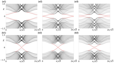
Figure 7: (Color online) The evolution of boundary energy gap on the upper $y$-normal edge with respect to $\mu$ for a cylindrical geometry with periodic boundary conditions in the $x$ direction. Chosen parameters are $t=1$, $\lambda_{\rm so}=0.1$, $M_{x}=M_{y}=0.2$, $\gamma=0.5$, $\lambda_{\nu}=0$ and $\Delta=0.1$. For (a1)-(a3), the open boundaries are beard edges, and the critical value of $\mu$ at which the boundary energy gap of the upper edge is equal to $0.265$ according to the chosen parameters. For (b1)-(b3), the open boundaries are zigzag edges, and the critical value of $\mu$ is equal to $0.077$. (a1) $\mu=0$, (a2) $\mu=0.265$, (a3) $\mu=0.35$, (b1) $\mu=0$, (b2) $\mu=0.07$, and (b3) $\mu=0.15$.

Without loss of generality, let us still focus on the regime $t\gg\lambda_{\rm so}$ so that $\eta\gg 1$ and the form of the low-energy boundary Hamiltonian on the zigzag edge can be simplified as

$$\mathcal{H}_{\rm BdG;z}(q_{x}^{\prime}) \approx v^{\prime}q_{x}^{\prime}\tau_{0}s_{z}-\gamma(M_{x}\tau_{z}s_{x}+M_{y}\tau_{0}s_{y})$$ (20)

$$-(\mu+\lambda_{\nu})\tau_{z}s_{0}-\Delta\tau_{y}s_{y}.$$

It is straightforward to find that the gap-closing condition of the boundary energy spectrum for the beard edge is

$$M=\sqrt{(\mu-\lambda_{\nu})^{2}+\Delta^{2}},$$ (21)

and for the zigzag edge, the gap-closing condition is

$$|\gamma|M=\sqrt{(\mu+\lambda_{\nu})^{2}+\Delta^{2}},$$ (22)

where $M=\sqrt{M_{x}^{2}+M_{y}^{2}}$. It is worth noting that, for simplicity, the gap-closing condition for the zigzag edge is obtained via the approximate Hamiltonian (20). The accurate condition can also be easily obtained according to the Hamiltonian (19), but will have a somewhat more complex expression (see Eq.(65)). In Fig.7, we assume that the exchange field is fixed, and show the evolution of the boundary energy spectra (red solid lines) with respect to $\mu$. We find that the critical $\mu_{c}$ at which the boundary energy gap on the upper edge gets closed agrees excellently with the value predicted by the low-energy boundary Hamiltonians (18) and (19), reflecting the power of the edge theory in describing the boundary physics.

For a given edge, the gap closure of the boundary energy spectrum signals a change of the boundary topology. For the upper beard edge, its Dirac mass falls into the superconductivity-dominated region when $M<M_{c,b}\equiv\sqrt{(\mu-\lambda_{\nu})^{2}+\Delta^{2}}$, and the exchange-field-dominated region when $M>M_{c,b}$. Similarly, the Dirac mass of the upper zigzag edge falls into the superconductivity-dominated region when $|\gamma|M<M_{c,z}\equiv\sqrt{(\mu+\lambda_{\nu})^{2}+\Delta^{2}}$, and the exchange-field-dominated region when $|\gamma|M>M_{c,z}$. When the Dirac masses on the upper beard and zigzag edges fall into different regions, the sublattice domain walls will bind MZMs.

Without loss of generality, let us consider $\mu\geq 0$ and $\lambda_{\nu}\geq 0$ to exemplify the physics. With this choice, the condition to realize MZMs at the sublattice domain walls is

$$M>M_{c,b},\quad|\gamma|M<M_{c,z}.$$ (23)

Since the two inequalities above are independent of the sign of $\gamma$, it indicates that MZMs at sublattice domain walls can be achieved for both ferromagnetic and antiferromagnetic exchange fields as long as the two inequalities are simultaneously fulfilled.

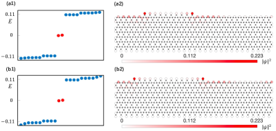
Figure 8: (Color online) Tunable MZMs at sublattice domain walls for a ferromagnetic exchange field. Chosen parameters are $t=1$, $\lambda_{\rm so}=0.1$, $M_{x}=M_{y}=0.2$, $\gamma=1$, $\Delta=0.15$, $\lambda_{\nu}=0.2$, and $\mu=0.2$. The geometry considered is depicted in (a2) and (b2), and a few corresponding eigenenergies near zero energy are shown in (a1) and (b1). Periodic boundary conditions are imposed in the $x$ direction. The red dots in the energy spectra denote MZMs (their energies are not exactly zero due to splitting induced by finite-size effects) at the sublattice domain walls. The right panels show their probability density profiles with the shade of the red color on the lattice sites reflecting the weight.

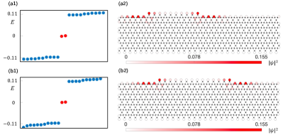
Figure 9: (Color online) Tunable MZMs at sublattice domain walls for an antiferromagnetic exchange field. All parameters are the same as in Fig.8 except $\gamma=-1$.

We would like to make a further remark on Eq.(23). The two inequalities suggest that the topological region supporting MZMs can be made very sizable. For instance, by tuning $\mu=\lambda_{\nu}$, $\gamma=0$, MZMs can be realized once $M>|\Delta|$. In Fig.8, we consider a ferromagnetic exchange field and show the realization of MZMs at the sublattice domain walls for a sample with cylindrical geometry (left and right edges are connected, hence there is no sharp corner). By a comparison of Fig.8(a2) and Fig.8(b2), it is easy to see that the positions of MZMs can be tuned to any place on the upper edge by manipulating the boundary sublattice terminations. Apparently, one can also manipulate two sublattice domain walls to move toward each other, then one can study the splitting and annihilation of two MZMs. In Fig.9, we consider an antiferromagnetic exchange field and show explicitly that the physics is similar.

VI Discussion and Conclusion

In this paper, we have shown when the lattice structure has sublattice degrees of freedom, the bound states in second-order TIs and TSCs are unnecessarily pinned at some specific sharp corners. By adjusting the boundary sublattice terminations to form sublattice domain walls, we have shown that the positions of the bound states can be freely manipulated. For the honeycomb lattice considered, if one designs a sample with the diamond shape as considered in Ref.Ren et al. (2020) or also with the honeycomb shape so that all edges take either the beard-type or the zigzag-type sublattice termination, then the sublattice domain walls allow to form at any place on the boundary. Accordingly, the positions of the bound states can be manipulated to any place on the boundary. It is reasonable to expect that such a sublattice-enriched tunability would benefit the manipulation and application of the bound states, e.g., braiding MZMs Zhang et al. (2020a, b); Pahomi et al. (2020).

About the experimental implementation, we would like to first emphasize that our predictions are relevant to both quantum materials and classical systems. For quantum-material realization, one route is to apply a magnetic field to a two-dimensional first-order TI described by the Kane-Mele model, such as silicene, germanene, stanene Liu et al. (2011a, b); Ezawa (2012). As twisted transition metal dichalcogenide homobilayers are predicted to effectively realize Kane-Mele model and allow various types of magnetic orders Wu et al. (2019b); Zare and Mosadeq (2021), they may also serve as a platform to explore the predicted boundary physics. Another route is to find intrinsic magnetic second-order TI with sublattice degrees of freedom through first-principle calculations Chen et al. (2020b); Luo et al. (2022); Mu et al. (2022). Generalizations to the superconducting counterpart can be simply achieved by putting the above two classes of systems in proximity to a superconductor Yan (2019c); Wu et al. (2020a), as demonstrated in Sect.V. In quantum materials, as the lattice constant is at the atomic length scale, adjusting boundary sublattice terminations requires sophisticated tools, e.g., scanning tunneling microscope or scanning force microscope Stroscio and Eigler (1991); Custance et al. (2009). For classical-system realization, since the Kane-Mele model subjected to an in-plane Zeeman field has been effectively realized in an acoustic systemHuang et al. (2022), our prediction on the realization of bound states at sublattice domain walls in a second-order TI can be immediately explored. It is worth emphasizing that the manipulation of bound states at sublattice domain walls is expected to be much easier in classical systems than in quantum materials due to their much larger length scales. For instance, one can simply remove one sublattice on the boundary in an electric circuit by just removing all wires connected to that sublattice. As a final remark, it is worth pointing out that since the wave functions of the helical edge states decay exponentially away from the boundary, the boundary Dirac masses are mainly contributed by the exchange field and superconductivity at the neighborhood of the edges. In other words, the predicted boundary physics in this work can also be realized even when the exchange field and superconductivity are nonuniform or only appear at the neighborhood of the edges.

In summary, we have shown that the sublattice degrees of freedom and second-order topology have an interesting interplay, which can lead to the presence of rich boundary physics, such as the formation of highly controllable bound states.

VII Acknowledgements

D.Z. and Z.Y. are supported by the National Natural Science Foundation of China (Grant No.11904417 and No. 12174455) and the Natural Science Foundation of Guangdong Province (Grant No. 2021B1515020026). M.Kh is supported by the NSERC of Canada.

Appendix A Low-energy boundary Hamiltonian on the beard edge

The low-energy boundary Hamiltonians on the beard and zigzag edges for the Kane-Mele model have been derived in a previous work of us Zhu et al. (2022), but there we did not consider the staggered potential and exchange field. Here for self-consistency, we provide the main steps of the derivation.

Start with the BdG Hamiltonian in the momentum space,

$$\mathcal{H}_{\rm BdG}(\boldsymbol{k}) = t(2\cos\frac{\sqrt{3}k_{x}}{2}\cos\frac{k_{y}}{2}+\cos k_{y})\tau_{z}s_{0}\sigma_{x}$$ (24)

$$-t(2\cos\frac{\sqrt{3}k_{x}}{2}\sin\frac{k_{y}}{2}-\sin k_{y})\tau_{z}s_{0}\sigma_{y}$$

$$+2\lambda_{\rm so}(\sin\sqrt{3}k_{x}-2\sin\frac{\sqrt{3}k_{x}}{2}\cos\frac{3k_{y}}{2})\tau_{0}s_{z}\sigma_{z}$$

$$+\lambda_{\nu}\tau_{z}s_{0}\sigma_{z}-\mu\tau_{z}s_{0}\sigma_{0}$$

$$+\frac{1+\gamma}{2}(M_{x}\tau_{z}s_{x}+M_{y}\tau_{0}s_{y})\sigma_{0}$$

$$+\frac{1-\gamma}{2}(M_{x}\tau_{z}s_{x}+M_{y}\tau_{0}s_{y})\sigma_{z}$$

$$-\Delta\tau_{y}s_{y}\sigma_{0},$$

where $\tau_{i}$, $s_{i}$ and $\sigma_{i}$ are Pauli matrices acting on the particle-hole, spin and sublattice degrees of freedom, respectively, and $\tau_{0}$, $s_{0}$ and $\sigma_{0}$ denote identity matrices in the respective subspaces. For notational simplicity, the nearest-neighbor lattice constant has been set to unity.

When the upper boundary is a beard edge, the numerical results show that the corresponding boundary Dirac point is located at the time-reversal invariant momentum $k_{x}=0$ in the reduced boundary Brillouin zone. To derive the low-energy boundary Hamiltonian in an analytical way, we expand the bulk Hamiltonian around $k_{x}=0$ up to the linear order in momentum (the expansion is only performed in the $k_{x}$ direction), leading to

$$\mathcal{H}_{\rm BdG}(q_{x},k_{y}) = t(2\cos\frac{k_{y}}{2}+\cos k_{y})\tau_{z}s_{0}\sigma_{x}$$ (25)

$$-t(2\sin\frac{k_{y}}{2}-\sin k_{y})\tau_{z}s_{0}\sigma_{y}$$

$$+2\sqrt{3}\lambda_{\rm so}q_{x}(1-\cos\frac{3k_{y}}{2})\tau_{0}s_{z}\sigma_{z}$$

$$+\lambda_{\nu}\tau_{z}s_{0}\sigma_{z}-\mu\tau_{z}s_{0}\sigma_{0}$$

$$+\frac{1+\gamma}{2}(M_{x}\tau_{z}s_{x}+M_{y}\tau_{0}s_{y})\sigma_{0}$$

$$+\frac{1-\gamma}{2}(M_{x}\tau_{z}s_{x}+M_{y}\tau_{0}s_{y})\sigma_{z}$$

$$-\Delta\tau_{y}s_{y}\sigma_{0},$$

where $q_{x}$ denotes a small momentum which is measured from $k_{x}=0$. In the next step, we decompose the Hamiltonian into two parts, $\mathcal{H}_{\rm BdG}=\mathcal{H}_{0}+\mathcal{H}_{1}$, with

$$\mathcal{H}_{0}(q_{x},k_{y}) = t(2\cos\frac{k_{y}}{2}+\cos k_{y})\tau_{z}s_{0}\sigma_{x}$$

$$-t(2\sin\frac{k_{y}}{2}-\sin k_{y})\tau_{z}s_{0}\sigma_{y},$$

$$\mathcal{H}_{1}(q_{x},k_{y}) = 2\sqrt{3}\lambda_{so}q_{x}(1-\cos\frac{3k_{y}}{2})\tau_{0}s_{z}\sigma_{z}$$ (26)

$$+\lambda_{\nu}\tau_{z}s_{0}\sigma_{z}-\mu\tau_{z}s_{0}\sigma_{0}$$

$$+\frac{1+\gamma}{2}(M_{x}\tau_{z}s_{x}+M_{y}\tau_{0}s_{y})\sigma_{0}$$

$$+\frac{1-\gamma}{2}(M_{x}\tau_{z}s_{x}+M_{y}\tau_{0}s_{y})\sigma_{z}$$

$$-\Delta\tau_{y}s_{y}\sigma_{0}.$$

We will treat $\mathcal{H}_{1}$ as a perturbation, which is justified at least when the parameters in $\mathcal{H}_{1}$ are all much smaller than $t$. One can see that the two terms in $\mathcal{H}_{0}$ have a momentum dependence similar to the Su-Schrieffer-Heeger (SSH) model Su et al. (1979), but with the dimension of the Hamiltonian being increased from $2$ to $8$. On the other hand, $\mathcal{H}_{0}$ is independent of $q_{x}$. This implies that each $y$-normal edge may harbor a zero-energy flat band with four-fold degeneracy if periodic boundary conditions are imposed in the $x$ direction. To confirm this, we focus on the upper $y$-normal edge for illustration.

To simplify the derivation, we consider a half-infinity sample with the boundary corresponding to the upper beard edge. Accordingly, a natural basis is $\Psi_{q_{x}}=(c_{1,A,q_{x}},c_{1,B,q_{x}},c_{2,A,q_{x}},c_{2,B,q_{x}},...,c_{n,A,q_{x}},c_{n,B,q_{x}},...)^{T}$ with $c_{n,\alpha,q_{x}}=(c_{n,\alpha,q_{x},\uparrow},c_{n,\alpha,q_{x},\downarrow},c_{n,\alpha,-q_{x},\uparrow}^{{\dagger}},c_{n,\alpha,-q_{x},\downarrow}^{{\dagger}})$, where $\alpha=\{A,B\}$. Under this basis, the matrix form of $\mathcal{H}_{0}$ reads

$$\mathcal{H}_{0}=\left(\begin{array}[]{cccccc}0&t\tau_{z}s_{0}&0&0&0&\cdots\\ t\tau_{z}s_{0}&0&2t\tau_{z}s_{0}&0&0&\cdots\\ 0&2t\tau_{z}s_{0}&0&t\tau_{z}s_{0}&0&\cdots\\ 0&0&t\tau_{z}s_{0}&0&2t\tau_{z}s_{0}&\cdots\\ 0&0&0&2t\tau_{z}s_{0}&0&\cdots\\ \vdots&\vdots&\vdots&\vdots&\vdots&\ddots\\ \end{array}\right).\,$$ (33)

Here each “0” element denotes a four-by-four null matrix. The wave functions of the zero-energy bound states are determined by solving the eigenvalue equation $\mathcal{H}_{0}|\Psi_{\alpha}\rangle=0$. By observation, one can notice that $\tau_{z}$ and $s_{z}$ both commute with $\mathcal{H}_{0}$, so $|\Psi_{\alpha}\rangle$ can be assigned with the form

$$|\Psi_{\tau s}\rangle=(\psi_{1A},\psi_{1B},\psi_{2A},\psi_{2B},...)^{T}\otimes|\tau_{z}=\tau\rangle\otimes|s_{z}=s\rangle,\qquad$$ (34)

where $|\tau_{z}=\tau\rangle$ and $|s_{z}=s\rangle$ with $\tau=\pm 1$ and $s=\pm 1$ correspond to the two eigenstates of $\tau_{z}$ and $s_{z}$, respectively. Solving the eigenvalue equation $\mathcal{H}_{0}|\Psi_{\tau s}\rangle=0$ is equivalent to solving the following iterative equations,

$$t\psi_{1B}=0,$$

$$t\psi_{1A}+2t\psi_{2A}=0,$$

$$2t\psi_{1B}+t\psi_{2B}=0,$$

$$...$$

$$t\psi_{nA}+2t\psi_{(n+1)A}=0,$$

$$2t\psi_{nB}+t\psi_{(n+1)B}=0,$$

$$...,$$ (35)

According to the iterative structure, it is easy to find

$$\psi_{(n+1)A}=-\frac{1}{2}\psi_{nA},\quad\psi_{nB}=0.$$ (36)

Therefore, the eigenvectors take the form

$$|\Psi_{\tau s}\rangle = \mathcal{N}(1,0,-\frac{1}{2},0,...,(-\frac{1}{2})^{(n-1)},0,...)^{T}$$ (37)

$$\otimes|\tau_{z}=\tau\rangle\otimes|s_{z}=s\rangle,$$

where $\mathcal{N}$ denotes the normalization constant. According to the normalization condition $\langle\Psi_{\tau s}|\Psi_{\tau s}\rangle=1$, simple calculations reveal

$$\mathcal{N}^{2}\sum_{n=0}^{\infty}\frac{1}{2^{2n}}=\mathcal{N}^{2}\frac{1}{1-\frac{1}{4}}=\frac{4}{3}\mathcal{N}^{2}=1,$$ (38)

so $\mathcal{N}=\frac{\sqrt{3}}{2}$. As $\psi_{nA}$ decays exponentially with the increase of $n$, the existence of four such eigenvectors indicates the existence of four zero-energy bound states, confirming the correctness of the simple analysis based on the connection to SSH model. It is worth noting that the TI has only one pair of gapless helical states on a given edge, so there should exist only two degenerate zero-energy bound states at $q_{x}=0$. Here the existence of four zero-energy bound states originates from the doubling due to the introduction of particle-hole redundancy. The low-energy Hamiltonian on the upper $y$-normal beard edge is then obtained by projecting $\mathcal{H}_{1}$ onto the four-dimensional subspace spanned by the four orthogonal eigenstates. Put it explicitly, the matrix elements of the low-energy boundary Hamiltonian are given by

$$[\mathcal{H}_{\rm BdG,b}(q_{x})]_{\tau s,\tau^{\prime}s^{\prime}}=\langle\Psi_{\tau s}|\mathcal{H}_{1}(q_{x})|\Psi_{\tau^{\prime}s^{\prime}}\rangle.$$ (39)

It is worth noting that here $\mathcal{H}_{1}(q_{x})$ is also an infinitely large matrix, and its form is given by a partial Fourier transform of $\mathcal{H}_{1}(q_{x},k_{y})$ in the $y$ direction. By some straightforward calculations and choosing $(|\Psi_{11}\rangle,|\Psi_{1-1}\rangle,|\Psi_{-11}\rangle,|\Psi_{-1-1}\rangle)^{T}$ as the basis for the low-energy boundary Hamiltonian, one can obtain (more details on how to determine each term in the low-energy Hamiltonian can be found in Ref. Zhu et al. (2022))

$$\mathcal{H}_{\rm BdG,b}(q_{x}) = vq_{x}\tau_{0}s_{z}+M_{x}\tau_{z}s_{x}+M_{y}\tau_{0}s_{y}$$ (40)

$$-(\mu-\lambda_{\nu})\tau_{z}s_{0}-\Delta\tau_{y}s_{y},$$

where $v=3\sqrt{3}\lambda_{\rm so}$. Without the superconductivity (the particle-hole redundancy is accordingly removed) and staggered potential, the low-energy boundary Hamiltonian reduces to the form in Eq.(11). The boundary energy spectra associated with this boundary Hamiltonian read

$$E(q_{x})=\pm\sqrt{F\pm 2\sqrt{G}},$$ (41)

where $F=v^{2}q_{x}^{2}+M^{2}+(\mu-\lambda_{\nu})^{2}+\Delta^{2}$ and $G=(\mu-\lambda_{\nu})^{2}(v^{2}q_{x}^{2}+M^{2})+M^{2}\Delta^{2}$. The gap of the boundary energy spectra gets closed at $q_{x}=0$ when the following condition is fulfilled,

$$M=\sqrt{(\mu-\lambda_{\nu})^{2}+\Delta^{2}}.$$ (42)

Appendix B Low-energy boundary Hamiltonian on the zigzag edge

Following the same spirit, we can derive the low-energy boundary Hamiltonian on the upper $y$-normal zigzag edge. Since numerical results show that the boundary Dirac point on the $y$-normal zigzag edge is located at $k_{x}=\pi/\sqrt{3}$, we similarly expand the Hamiltonian up to the linear order in momentum, which then gives

$$\mathcal{H}_{\rm BdG}(q_{x}^{\prime},k_{y}) = t(-\sqrt{3}q_{x}^{\prime}\cos\frac{k_{y}}{2}+\cos k_{y})\tau_{z}s_{0}\sigma_{x}$$ (43)

$$+t(\sqrt{3}q_{x}^{\prime}\sin\frac{k_{y}}{2}+\sin k_{y})\tau_{z}s_{0}\sigma_{y}$$

$$+2\lambda_{\rm so}(-\sqrt{3}q_{x}^{\prime}-2\cos\frac{3k_{y}}{2})\tau_{0}s_{z}\sigma_{z}$$

$$+\lambda_{\nu}\tau_{z}s_{0}\sigma_{z}-\mu\tau_{z}s_{0}\sigma_{0}$$

$$+\frac{1+\gamma}{2}(M_{x}\tau_{z}s_{x}+M_{y}\tau_{0}s_{y})\sigma_{0}$$

$$+\frac{1-\gamma}{2}(M_{x}\tau_{z}s_{x}+M_{y}\tau_{0}s_{y})\sigma_{z}$$

$$-\Delta\tau_{y}s_{y}\sigma_{0},$$

where $q_{x}^{\prime}$ denotes a small momentum measured from $k_{x}=\pi/\sqrt{3}$. Similarly, we decompose the Hamiltonian into two parts, $\mathcal{H}=\mathcal{H}_{0}+\mathcal{H}_{1}$, with

$$\mathcal{H}_{0}(q_{x}^{\prime},k_{y}) = t\cos k_{y}\tau_{z}s_{0}\sigma_{x}+t\sin k_{y}\tau_{z}s_{0}\sigma_{y}$$

$$-4\lambda_{\rm so}\cos\frac{3k_{y}}{2}\tau_{0}s_{z}\sigma_{z},$$

$$\mathcal{H}_{1}(q_{x}^{\prime},k_{y}) = -\sqrt{3}tq_{x}^{\prime}\cos\frac{k_{y}}{2}\tau_{z}s_{0}\sigma_{x}+\sqrt{3}tq_{x}^{\prime}\sin\frac{k_{y}}{2}\tau_{z}s_{0}\sigma_{y}$$ (44)

$$-2\sqrt{3}\lambda_{\rm so}q_{x}^{\prime}\tau_{0}s_{z}\sigma_{z}$$

$$+\lambda_{\nu}\tau_{z}s_{0}\sigma_{z}-\mu\tau_{z}s_{0}\sigma_{0}$$

$$+\frac{1+\gamma}{2}(M_{x}\tau_{z}s_{x}+M_{y}\tau_{0}s_{y})\sigma_{0}$$

$$+\frac{1-\gamma}{2}(M_{x}\tau_{z}s_{x}+M_{y}\tau_{0}s_{y})\sigma_{z}$$

$$-\Delta\tau_{y}s_{y}\sigma_{0}.$$

Also focusing on the upper $y$-normal boundary, the change from a beard edge to a zigzag edge is accompanied with the change of terminating sublattice from sublattice A to sublattice B. For simplicity, we also consider the half-infinity geometry, and then the corresponding basis becomes $\Psi_{q_{x}^{\prime}}=(c_{1,B,q_{x}^{\prime}},c_{2,A,q_{x}^{\prime}},c_{2,B,q_{x}^{\prime}},c_{3,A,q_{x}^{\prime}},c_{3,B,q_{x}^{\prime}},...)^{T}$. Under this basis, the corresponding matrix form of $\mathcal{H}_{0}$ reads

$$\mathcal{H}_{0}=\left(\begin{array}[]{cccccc}0&T_{1}&0&0&0&\cdots\\ T_{1}^{{\dagger}}&0&T_{1}&0&0&\cdots\\ 0&T_{1}^{{\dagger}}&0&T_{1}&0&\cdots\\ 0&0&T_{1}^{{\dagger}}&0&T_{1}&\cdots\\ 0&0&0&T_{1}^{{\dagger}}&0&\cdots\\ \vdots&\vdots&\vdots&\vdots&\vdots&\ddots\\ \end{array}\right),\,$$ (51)

where now each “0” element in $\mathcal{H}_{0}$ is an eight-by-eight null matrix, and

$$T_{1} = \left(\begin{array}[]{cc}2\lambda_{\rm so}\tau_{0}s_{z}&0\\ t\tau_{z}s_{0}&-2\lambda_{\rm so}\tau_{0}s_{z}\\ \end{array}\right).$$ (54)

As here $\tau_{z}$ and $s_{z}$ also commute with $\mathcal{H}_{0}$, the wave functions for zero-energy bound states can also be assigned with the from

$$|\Psi_{\tau s}\rangle = (\psi_{1B},\psi_{2A},\psi_{2B},\psi_{3A},\psi_{3B},...)^{T}$$ (55)

$$\otimes|\tau_{z}=\tau\rangle\otimes|s_{z}=s\rangle.$$

The eigenvalue equation $\mathcal{H}_{0}|\Psi_{\tau s}\rangle=0$ leads to the following iterative equations,

$$2\lambda_{\rm so,s}\psi_{2B}=0,$$

$$t_{\tau}\psi_{2B}-2\lambda_{\rm so,s}\psi_{3A}=0,$$

$$2\lambda_{\rm so,s}\psi_{1B}+t_{\tau}\psi_{2A}+2\lambda_{\rm so,s}\psi_{3B}=0,$$

$$-2\lambda_{\rm so,s}\psi_{2A}+t_{\tau}\psi_{3B}-2\lambda_{\rm so,s}\psi_{4A}=0,$$

$$...$$

$$2\lambda_{\rm so,s}\psi_{(n-1)B}+t_{\tau}\psi_{nA}+2\lambda_{\rm so,s}\psi_{(n+1)B}=0,$$

$$-2\lambda_{\rm so,s}\psi_{nA}+t_{\tau}\psi_{(n+1)B}-2\lambda_{\rm so,s}\psi_{(n+2)A}=0,$$

$$...,$$ (56)

where $t_{\tau}=t\tau$ and $\lambda_{\rm so,s}=\lambda_{\rm so}s$. The solutions are found to take the form (more details can be found in Ref. Zhu et al. (2022))

$$|\Psi_{\tau s}\rangle = \mathcal{N}(\eta_{\tau s},1,0,0,\xi\eta_{\tau s},\xi,0,0,\xi^{2}\eta_{\tau s},\xi^{2},...)^{T}$$ (57)

$$\otimes|\tau_{z}=\tau\rangle\otimes|s_{z}=s\rangle,$$

where

$$\xi = \frac{\sqrt{t^{2}(t^{2}+16\lambda_{\rm so}^{2})}-(t^{2}+8\lambda_{\rm so}^{2})}{8\lambda_{\rm so}^{2}},$$

$$\mathcal{N} = \sqrt{\frac{{1-\xi^{2}}}{1+\eta^{2}}},$$

$$\eta = \frac{4t\lambda_{\rm so}}{\sqrt{t^{2}(t^{2}+16\lambda_{\rm so}^{2})}-t^{2}},$$ (58)

and $\eta_{\tau s}=-\tau s\eta$. Similarly, projecting $\mathcal{H}_{1}$ onto the four-dimensional subspace spanned by the four orthogonal wave functions associated with the four zero-energy bound states, one can obtain the low-energy boundary Hamiltonian, which reads

$$\mathcal{H}_{\rm BdG;z}(q_{x}^{\prime}) = v^{\prime}q_{x}^{\prime}\tau_{0}s_{z}+\frac{1-\gamma\eta^{2}}{1+\eta^{2}}(M_{x}\tau_{z}s_{x}+M_{y}\tau_{0}s_{y})$$ (59)

$$-(\mu+\frac{\eta^{2}-1}{1+\eta^{2}}\lambda_{\nu})\tau_{z}s_{0}-\Delta\tau_{y}s_{y},$$

where

$$v^{\prime}=\frac{2\sqrt{3}t\eta+2\sqrt{3}\lambda_{so}(\eta^{2}-1)}{1+\eta^{2}}.$$ (60)

For real materials, it is common that $t\gg\lambda_{\rm so}$. When $t\gg\lambda_{\rm so}$, one finds

$$\eta = \frac{4t\lambda_{\rm so}}{\sqrt{t^{2}(t^{2}+16\lambda_{\rm so}^{2})}-t^{2}}$$ (61)

$$\approx \frac{4t\lambda_{\rm so}}{(t^{2}+8\lambda_{\rm so}^{2})-t^{2}}$$

$$= \frac{t}{2\lambda_{\rm so}}\gg 1.$$

In this limit, $v^{\prime}\approx 2v$, and the boundary Hamiltonian for the zigzag edge can be simplified as

$$\mathcal{H}_{\rm BdG;z}(q_{x}^{\prime}) \approx v^{\prime}q_{x}^{\prime}\tau_{0}s_{z}-\gamma(M_{x}\tau_{z}s_{x}+M_{y}\tau_{0}s_{y})$$ (62)

$$-(\mu+\lambda_{\nu})\tau_{z}s_{0}-\Delta\tau_{y}s_{y}.$$

The corresponding boundary energy spectra read

$$E(q_{x}^{\prime})=\pm\sqrt{F^{\prime}\pm 2\sqrt{G^{\prime}}},$$ (63)

where $F^{\prime}=v^{\prime 2}q_{x}^{2}+\gamma^{2}M^{2}+(\mu+\lambda_{\nu})^{2}+\Delta^{2}$ and $G^{\prime}=(\mu+\lambda_{\nu})^{2}(v^{\prime 2}q_{x}^{2}+\gamma^{2}M^{2})+\gamma^{2}M^{2}\Delta^{2}$. The gap of the boundary energy spectra gets closed at $q_{x}^{\prime}=0$ when the following condition is fulfilled,

$$|\gamma|M=\sqrt{(\mu+\lambda_{\nu})^{2}+\Delta^{2}}.$$ (64)

If one determines the gap-closing condition according to the Hamiltonian (59), one only needs to do the replacement, $\gamma\rightarrow(1-\gamma\eta^{2})/(1+\eta^{2})$, and $\lambda_{\nu}\rightarrow\lambda_{\nu}(\eta^{2}-1)/(1+\eta^{2})$, namely, the criterion (64) for gap closure is simply modified as

$$|\frac{1-\gamma\eta^{2}}{1+\eta^{2}}|M=\sqrt{(\mu+\frac{\eta^{2}-1}{1+\eta^{2}}\lambda_{\nu})^{2}+\Delta^{2}}.$$ (65)

References

- Kane and Mele (2005a) C. L. Kane and E. J. Mele, “Quantum spin Hall effect in graphene,” Phys. Rev. Lett. 95, 226801 (2005a).
- Kane and Mele (2005b) C. L. Kane and E. J. Mele, “ topological order and the quantum spin Hall effect,” Phys. Rev. Lett. 95, 146802 (2005b).
- Bernevig and Zhang (2006) B. Andrei Bernevig and Shou-Cheng Zhang, “Quantum spin Hall effect,” Phys. Rev. Lett. 96, 106802 (2006).
- Bernevig et al. (2006) B. Andrei Bernevig, Taylor L. Hughes, and Shou-Cheng Zhang, “Quantum spin Hall effect and topological phase transition in HgTe quantum wells,” Science 314, 1757–1761 (2006).
- König et al. (2007) Markus König, Steffen Wiedmann, Christoph Brüne, Andreas Roth, Hartmut Buhmann, Laurens W. Molenkamp, Xiao-Liang Qi, and Shou-Cheng Zhang, “Quantum spin Hall insulator state in HgTe quantum wells,” Science 318, 766–770 (2007).
- Hasan and Kane (2010) M. Z. Hasan and C. L. Kane, “Colloquium : Topological insulators,” Rev. Mod. Phys. 82, 3045–3067 (2010).
- Qi and Zhang (2011) Xiao-Liang Qi and Shou-Cheng Zhang, “Topological insulators and superconductors,” Rev. Mod. Phys. 83, 1057–1110 (2011).
- Ozawa et al. (2019) Tomoki Ozawa, Hannah M. Price, Alberto Amo, Nathan Goldman, Mohammad Hafezi, Ling Lu, Mikael C. Rechtsman, David Schuster, Jonathan Simon, Oded Zilberberg, and Iacopo Carusotto, “Topological photonics,” Rev. Mod. Phys. 91, 015006 (2019).
- Ma et al. (2019) Guancong Ma, Meng Xiao, and C. T. Chan, “Topological phases in acoustic and mechanical systems,” Nature Reviews Physics 1, 281–294 (2019).
- Chiu et al. (2016) Ching-Kai Chiu, Jeffrey C. Y. Teo, Andreas P. Schnyder, and Shinsei Ryu, “Classification of topological quantum matter with symmetries,” Rev. Mod. Phys. 88, 035005 (2016).
- Sitte et al. (2012) M. Sitte, A. Rosch, E. Altman, and L. Fritz, “Topological insulators in magnetic fields: Quantum Hall effect and edge channels with a nonquantized term,” Phys. Rev. Lett. 108, 126807 (2012).
- Zhang et al. (2013) Fan Zhang, C. L. Kane, and E. J. Mele, “Surface state magnetization and chiral edge states on topological insulators,” Phys. Rev. Lett. 110, 046404 (2013).
- Benalcazar et al. (2017a) Wladimir A. Benalcazar, B. Andrei Bernevig, and Taylor L. Hughes, “Quantized electric multipole insulators,” Science 357, 61–66 (2017a).
- Benalcazar et al. (2017b) Wladimir A. Benalcazar, B. Andrei Bernevig, and Taylor L. Hughes, “Electric multipole moments, topological multipole moment pumping, and chiral hinge states in crystalline insulators,” Phys. Rev. B 96, 245115 (2017b).
- Schindler et al. (2018a) Frank Schindler, Ashley M. Cook, Maia G. Vergniory, Zhijun Wang, Stuart S. P. Parkin, B. Andrei Bernevig, and Titus Neupert, “Higher-order topological insulators,” Science Advances 4, eaat0346 (2018a).
- Song et al. (2017) Zhida Song, Zhong Fang, and Chen Fang, “-dimensional edge states of rotation symmetry protected topological states,” Phys. Rev. Lett. 119, 246402 (2017).
- Langbehn et al. (2017) Josias Langbehn, Yang Peng, Luka Trifunovic, Felix von Oppen, and Piet W. Brouwer, “Reflection-symmetric second-order topological insulators and superconductors,” Phys. Rev. Lett. 119, 246401 (2017).
- Liu and Wakabayashi (2017) Feng Liu and Katsunori Wakabayashi, “Novel topological phase with a zero Berry curvature,” Phys. Rev. Lett. 118, 076803 (2017).
- Ezawa (2018) Motohiko Ezawa, “Higher-order topological insulators and semimetals on the breathing kagome and pyrochlore lattices,” Phys. Rev. Lett. 120, 026801 (2018).
- Geier et al. (2018) Max Geier, Luka Trifunovic, Max Hoskam, and Piet W. Brouwer, “Second-order topological insulators and superconductors with an order-two crystalline symmetry,” Phys. Rev. B 97, 205135 (2018).
- Khalaf (2018) Eslam Khalaf, “Higher-order topological insulators and superconductors protected by inversion symmetry,” Phys. Rev. B 97, 205136 (2018).
- Yan et al. (2018) Zhongbo Yan, Fei Song, and Zhong Wang, “Majorana corner modes in a high-temperature platform,” Phys. Rev. Lett. 121, 096803 (2018).
- Wang et al. (2018a) Qiyue Wang, Cheng-Cheng Liu, Yuan-Ming Lu, and Fan Zhang, “High-temperature Majorana corner states,” Phys. Rev. Lett. 121, 186801 (2018a).
- Wang et al. (2018b) Yuxuan Wang, Mao Lin, and Taylor L. Hughes, “Weak-pairing higher order topological superconductors,” Phys. Rev. B 98, 165144 (2018b).
- Yan (2019a) Zhongbo Yan, “Higher-order topological odd-parity superconductors,” Phys. Rev. Lett. 123, 177001 (2019a).
- Liu et al. (2019) Tao Liu, Yu-Ran Zhang, Qing Ai, Zongping Gong, Kohei Kawabata, Masahito Ueda, and Franco Nori, “Second-order topological phases in non-Hermitian systems,” Phys. Rev. Lett. 122, 076801 (2019).
- Kudo et al. (2019) Koji Kudo, Tsuneya Yoshida, and Yasuhiro Hatsugai, “Higher-order topological Mott insulators,” Phys. Rev. Lett. 123, 196402 (2019).
- Chen et al. (2020a) Rui Chen, Chui-Zhen Chen, Jin-Hua Gao, Bin Zhou, and Dong-Hui Xu, “Higher-order topological insulators in quasicrystals,” Phys. Rev. Lett. 124, 036803 (2020a).
- Huang and Liu (2020) Biao Huang and W. Vincent Liu, “Floquet higher-order topological insulators with anomalous dynamical polarization,” Phys. Rev. Lett. 124, 216601 (2020).
- Hu et al. (2020) Haiping Hu, Biao Huang, Erhai Zhao, and W. Vincent Liu, “Dynamical singularities of Floquet higher-order topological insulators,” Phys. Rev. Lett. 124, 057001 (2020).
- Zhang et al. (2021) Weixuan Zhang, Deyuan Zou, Qingsong Pei, Wenjing He, Jiacheng Bao, Houjun Sun, and Xiangdong Zhang, “Experimental observation of higher-order topological Anderson insulators,” Phys. Rev. Lett. 126, 146802 (2021).
- Yan (2019b) Zhongbo Yan, “Higher-order topological insulators and superconductors,” Acta Physica Sinica 68, 226101 (2019b).
- Schindler (2020) Frank Schindler, “Dirac equation perspective on higher-order topological insulators,” Journal of Applied Physics 128, 221102 (2020).
- Xie et al. (2021) Biye Xie, Hai-Xiao Wang, Xiujuan Zhang, Peng Zhan, Jian-Hua Jiang, Minghui Lu, and Yanfeng Chen, “Higher-order band topology,” Nature Reviews Physics 3, 520–532 (2021).
- Călugăru et al. (2019) Dumitru Călugăru, Vladimir Juričić, and Bitan Roy, “Higher-order topological phases: A general principle of construction,” Phys. Rev. B 99, 041301 (2019).
- Ren et al. (2020) Yafei Ren, Zhenhua Qiao, and Qian Niu, “Engineering corner states from two-dimensional topological insulators,” Phys. Rev. Lett. 124, 166804 (2020).
- Chen et al. (2020b) Cong Chen, Zhida Song, Jian-Zhou Zhao, Ziyu Chen, Zhi-Ming Yu, Xian-Lei Sheng, and Shengyuan A. Yang, “Universal approach to magnetic second-order topological insulator,” Phys. Rev. Lett. 125, 056402 (2020b).
- Huang et al. (2022) Xueqin Huang, Jiuyang Lu, Zhongbo Yan, Mou Yan, Weiyin Deng, Gang Chen, and Zhengyou Liu, “Acoustic higher-order topology derived from first-order with built-in Zeeman-like fields,” Science Bulletin 67, 488–494 (2022).
- Jackiw and Rebbi (1976) R. Jackiw and C. Rebbi, “Solitons with fermion number ,” Phys. Rev. D 13, 3398–3409 (1976).
- Shen (2013) Shun-Qing Shen, Topological Insulators: Dirac Equation in Condensed Matters, Vol. 174 (Springer Science & Business Media, 2013).
- Zhu (2018) Xiaoyu Zhu, “Tunable Majorana corner states in a two-dimensional second-order topological superconductor induced by magnetic fields,” Phys. Rev. B 97, 205134 (2018).
- Zhuang and Yan (2022) Zheng-Yang Zhuang and Zhongbo Yan, “Topological phase transitions and evolution of boundary states induced by Zeeman fields in second-order topological insulators,” Frontiers in Physics 10, 866347 (2022).
- Zhang et al. (2019a) Rui-Xing Zhang, William S. Cole, and S. Das Sarma, “Helical hinge Majorana modes in iron-based superconductors,” Phys. Rev. Lett. 122, 187001 (2019a).
- Kheirkhah et al. (2021) Majid Kheirkhah, Zhongbo Yan, and Frank Marsiglio, “Vortex-line topology in iron-based superconductors with and without second-order topology,” Phys. Rev. B 103, L140502 (2021).
- Kheirkhah et al. (2022a) Majid Kheirkhah, Zheng-Yang Zhuang, Joseph Maciejko, and Zhongbo Yan, “Surface Bogoliubov-Dirac cones and helical Majorana hinge modes in superconducting Dirac semimetals,” Phys. Rev. B 105, 014509 (2022a).
- Peterson et al. (2018) Christopher W. Peterson, Wladimir A. Benalcazar, Taylor L. Hughes, and Gaurav Bahl, “A quantized microwave quadrupole insulator with topologically protected corner states,” Nature 555, 346–350 (2018).
- Serra-Garcia et al. (2018) Marc Serra-Garcia, Valerio Peri, Roman Süsstrunk, Osama R. Bilal, Tom Larsen, Luis Guillermo Villanueva, and Sebastian D. Huber, “Observation of a phononic quadrupole topological insulator,” Nature 555, 342–345 (2018).
- Imhof et al. (2018) Stefan Imhof, Christian Berger, Florian Bayer, Johannes Brehm, Laurens W. Molenkamp, Tobias Kiessling, Frank Schindler, Ching Hua Lee, Martin Greiter, Titus Neupert, and Ronny Thomale, “Topolectrical-circuit realization of topological corner modes,” Nature Physics 14, 925–929 (2018).
- Zhang et al. (2019b) Xiujuan Zhang, Hai-Xiao Wang, Zhi-Kang Lin, Yuan Tian, Biye Xie, Ming-Hui Lu, Yan-Feng Chen, and Jian-Hua Jiang, “Second-order topology and multidimensional topological transitions in sonic crystals,” Nature Physics 15, 582–588 (2019b).
- Chen et al. (2019) Xiao-Dong Chen, Wei-Min Deng, Fu-Long Shi, Fu-Li Zhao, Min Chen, and Jian-Wen Dong, “Direct observation of corner states in second-order topological photonic crystal slabs,” Phys. Rev. Lett. 122, 233902 (2019).
- Fan et al. (2019) Haiyan Fan, Baizhan Xia, Liang Tong, Shengjie Zheng, and Dejie Yu, “Elastic higher-order topological insulator with topologically protected corner states,” Phys. Rev. Lett. 122, 204301 (2019).
- El Hassan et al. (2019) Ashraf El Hassan, Flore K. Kunst, Alexander Moritz, Guillermo Andler, Emil J. Bergholtz, and Mohamed Bourennane, “Corner states of light in photonic waveguides,” Nature Photonics 13, 697–700 (2019).
- Schindler et al. (2018b) Frank Schindler, Zhijun Wang, Maia G. Vergniory, Ashley M. Cook, Anil Murani, Shamashis Sengupta, Alik Yu. Kasumov, Richard Deblock, Sangjun Jeon, Ilya Drozdov, Hélène Bouchiat, Sophie Guéron, Ali Yazdani, B. Andrei Bernevig, and Titus Neupert, “Higher-order topology in bismuth,” Nature Physics 14, 918–924 (2018b).
- Gray et al. (2019) Mason J. Gray, Josef Freudenstein, Shu Yang F. Zhao, Ryan O’Connor, Samuel Jenkins, Narendra Kumar, Marcel Hoek, Abigail Kopec, Soonsang Huh, Takashi Taniguchi, Kenji Watanabe, Ruidan Zhong, Changyoung Kim, G. D. Gu, and K. S. Burch, “Evidence for helical hinge zero modes in an Fe-based superconductor,” Nano Letters 19, 4890–4896 (2019).
- Choi et al. (2020) Yong-Bin Choi, Yingming Xie, Chui-Zhen Chen, Jinho Park, Su-Beom Song, Jiho Yoon, B. J. Kim, Takashi Taniguchi, Kenji Watanabe, Jonghwan Kim, Kin Chung Fong, Mazhar N. Ali, Kam Tuen Law, and Gil-Ho Lee, “Evidence of higher-order topology in multilayer WTe2 from josephson coupling through anisotropic hinge states,” Nature Materials 19, 974–979 (2020).
- Noguchi et al. (2021) Ryo Noguchi, Masaru Kobayashi, Zhanzhi Jiang, Kenta Kuroda, Takanari Takahashi, Zifan Xu, Daehun Lee, Motoaki Hirayama, Masayuki Ochi, Tetsuroh Shirasawa, Peng Zhang, Chun Lin, Cédric Bareille, Shunsuke Sakuragi, Hiroaki Tanaka, So Kunisada, Kifu Kurokawa, Koichiro Yaji, Ayumi Harasawa, Viktor Kandyba, Alessio Giampietri, Alexei Barinov, Timur K. Kim, Cephise Cacho, Makoto Hashimoto, Donghui Lu, Shik Shin, Ryotaro Arita, Keji Lai, Takao Sasagawa, and Takeshi Kondo, “Evidence for a higher-order topological insulator in a three-dimensional material built from van der Waals stacking of bismuth-halide chains,” Nature Materials 20, 473–479 (2021).
- Aggarwal et al. (2021) Leena Aggarwal, Penghao Zhu, Taylor L. Hughes, and Vidya Madhavan, “Evidence for higher order topology in Bi and Bi0.92Sb0.08,” Nature Communications 12, 4420 (2021).
- Shumiya et al. (2022) Nana Shumiya, Md Shafayat Hossain, Jia-Xin Yin, Zhiwei Wang, Maksim Litskevich, Chiho Yoon, Yongkai Li, Ying Yang, Yu-Xiao Jiang, Guangming Cheng, Yen-Chuan Lin, Qi Zhang, Zi-Jia Cheng, Tyler A. Cochran, Daniel Multer, Xian P. Yang, Brian Casas, Tay-Rong Chang, Titus Neupert, Zhujun Yuan, Shuang Jia, Hsin Lin, Nan Yao, Luis Balicas, Fan Zhang, Yugui Yao, and M. Zahid Hasan, “Evidence of a room-temperature quantum spin Hall edge state in a higher-order topological insulator,” Nature Materials 21, 1111–1115 (2022).
- Zhu et al. (2022) Di Zhu, Bo-Xuan Li, and Zhongbo Yan, “Sublattice-sensitive majorana modes,” Phys. Rev. B 106, 245418 (2022).
- Kheirkhah et al. (2022b) Majid Kheirkhah, Di Zhu, Joseph Maciejko, and Zhongbo Yan, “Corner- and sublattice-sensitive Majorana zero modes on the kagome lattice,” Phys. Rev. B 106, 085420 (2022b).
- Haim and Oreg (2019) Arbel Haim and Yuval Oreg, “Time-reversal-invariant topological superconductivity in one and two dimensions,” Physics Reports 825, 1 – 48 (2019).
- Nayak et al. (2008) Chetan Nayak, Steven H. Simon, Ady Stern, Michael Freedman, and Sankar Das Sarma, “Non-Abelian anyons and topological quantum computation,” Rev. Mod. Phys. 80, 1083–1159 (2008).
- Liu et al. (2014) Xiong-Jun Liu, Chris L. M. Wong, and K. T. Law, “Non-Abelian Majorana doublets in time-reversal-invariant topological superconductors,” Phys. Rev. X 4, 021018 (2014).
- Gao et al. (2016) Pin Gao, Ying-Ping He, and Xiong-Jun Liu, “Symmetry-protected non-Abelian braiding of Majorana Kramers pairs,” Phys. Rev. B 94, 224509 (2016).
- Schrade and Fu (2018) Constantin Schrade and Liang Fu, “Quantum Computing with Majorana Kramers Pairs,” arXiv e-prints , arXiv:1807.06620 (2018), arXiv:1807.06620 [cond-mat.mes-hall] .
- Yu et al. (2010) Rui Yu, Wei Zhang, Hai-Jun Zhang, Shou-Cheng Zhang, Xi Dai, and Zhong Fang, “Quantized anomalous Hall effect in magnetic topological insulators,” Science 329, 61–64 (2010).
- Castro Neto et al. (2009) A. H. Castro Neto, F. Guinea, N. M. R. Peres, K. S. Novoselov, and A. K. Geim, “The electronic properties of graphene,” Rev. Mod. Phys. 81, 109–162 (2009).
- Haldane (1988) F. D. M. Haldane, “Model for a quantum Hall effect without landau levels: Condensed-matter realization of the “parity anomaly”,” Phys. Rev. Lett. 61, 2015–2018 (1988).
- Schnyder et al. (2008) Andreas P. Schnyder, Shinsei Ryu, Akira Furusaki, and Andreas W. W. Ludwig, “Classification of topological insulators and superconductors in three spatial dimensions,” Phys. Rev. B 78, 195125 (2008).
- Kitaev (2009) Alexei Kitaev, “Periodic table for topological insulators and superconductors,” AIP conference proceedings, 1134, 22–30 (2009).
- Ryu et al. (2010) Shinsei Ryu, Andreas P Schnyder, Akira Furusaki, and Andreas W W Ludwig, “Topological insulators and superconductors: tenfold way and dimensional hierarchy,” New Journal of Physics 12, 065010 (2010).
- Fu and Kane (2009) Liang Fu and C. L. Kane, “Josephson current and noise at a superconductor/quantum-spin-Hall-insulator/superconductor junction,” Phys. Rev. B 79, 161408 (2009).
- Yan (2019c) Zhongbo Yan, “Majorana corner and hinge modes in second-order topological insulator/superconductor heterostructures,” Phys. Rev. B 100, 205406 (2019c).
- Jäck et al. (2019) Berthold Jäck, Yonglong Xie, Jian Li, Sangjun Jeon, B. Andrei Bernevig, and Ali Yazdani, “Observation of a Majorana zero mode in a topologically protected edge channel,” Science 364, 1255–1259 (2019).
- Wu et al. (2020a) Ya-Jie Wu, Junpeng Hou, Yun-Mei Li, Xi-Wang Luo, Xiaoyan Shi, and Chuanwei Zhang, “In-plane Zeeman-field-induced Majorana corner and hinge modes in an -wave superconductor heterostructure,” Phys. Rev. Lett. 124, 227001 (2020a).
- Liu et al. (2018) Tao Liu, James Jun He, and Franco Nori, “Majorana corner states in a two-dimensional magnetic topological insulator on a high-temperature superconductor,” Phys. Rev. B 98, 245413 (2018).
- Zhang et al. (2019c) Rui-Xing Zhang, William S. Cole, Xianxin Wu, and S. Das Sarma, “Higher-order topology and nodal topological superconductivity in Fe(Se,Te) heterostructures,” Phys. Rev. Lett. 123, 167001 (2019c).
- Pan et al. (2019) Xiao-Hong Pan, Kai-Jie Yang, Li Chen, Gang Xu, Chao-Xing Liu, and Xin Liu, “Lattice-symmetry-assisted second-order topological superconductors and Majorana patterns,” Phys. Rev. Lett. 123, 156801 (2019).
- Kheirkhah et al. (2020a) Majid Kheirkhah, Yuki Nagai, Chun Chen, and Frank Marsiglio, “Majorana corner flat bands in two-dimensional second-order topological superconductors,” Phys. Rev. B 101, 104502 (2020a).
- Laubscher et al. (2020) Katharina Laubscher, Danial Chughtai, Daniel Loss, and Jelena Klinovaja, “Kramers pairs of Majorana corner states in a topological insulator bilayer,” Phys. Rev. B 102, 195401 (2020).
- Li and Yan (2021) Bo-Xuan Li and Zhongbo Yan, “Boundary topological superconductors,” Phys. Rev. B 103, 064512 (2021).
- Li and Zhou (2021) Yu-Xuan Li and Tao Zhou, “Rotational symmetry breaking and partial Majorana corner states in a heterostructure based on high- superconductors,” Phys. Rev. B 103, 024517 (2021).
- Tan et al. (2022) Yi Tan, Zhi-Hao Huang, and Xiong-Jun Liu, “Two-particle Berry phase mechanism for Dirac and Majorana Kramers pairs of corner modes,” Phys. Rev. B 105, L041105 (2022).
- Wu et al. (2022) Ya-Jie Wu, Wei Tu, and Ning Li, “Majorana corner states in an attractive quantum spin Hall insulator with opposite in-plane Zeeman energy at two sublattice sites,” Journal of Physics: Condensed Matter 34, 375601 (2022).
- Wu et al. (2019a) Zhigang Wu, Zhongbo Yan, and Wen Huang, “Higher-order topological superconductivity: Possible realization in Fermi gases and Sr2RuO4,” Phys. Rev. B 99, 020508 (2019a).
- Ikegaya et al. (2021) S. Ikegaya, W. B. Rui, D. Manske, and Andreas P. Schnyder, “Tunable Majorana corner modes in noncentrosymmetric superconductors: Tunneling spectroscopy and edge imperfections,” Phys. Rev. Research 3, 023007 (2021).
- Roy (2020) Bitan Roy, “Higher-order topological superconductors in -, -odd quadrupolar dirac materials,” Phys. Rev. B 101, 220506 (2020).
- Zhu (2019) Xiaoyu Zhu, “Second-order topological superconductors with mixed pairing,” Phys. Rev. Lett. 122, 236401 (2019).
- Kheirkhah et al. (2020b) Majid Kheirkhah, Zhongbo Yan, Yuki Nagai, and Frank Marsiglio, “First- and second-order topological superconductivity and temperature-driven topological phase transitions in the extended Hubbard model with spin-orbit coupling,” Phys. Rev. Lett. 125, 017001 (2020b).
- Ahn and Yang (2020) Junyeong Ahn and Bohm-Jung Yang, “Higher-order topological superconductivity of spin-polarized fermions,” Phys. Rev. Research 2, 012060 (2020).
- Hsu et al. (2020) Yi-Ting Hsu, William S. Cole, Rui-Xing Zhang, and Jay D. Sau, “Inversion-protected higher-order topological superconductivity in monolayer WTe2,” Phys. Rev. Lett. 125, 097001 (2020).
- Li et al. (2021) Tommy Li, Max Geier, Julian Ingham, and Harley D Scammell, “Higher-order topological superconductivity from repulsive interactions in kagome and honeycomb systems,” 2D Materials 9, 015031 (2021).
- Scammell et al. (2022) Harley D. Scammell, Julian Ingham, Max Geier, and Tommy Li, “Intrinsic first- and higher-order topological superconductivity in a doped topological insulator,” Phys. Rev. B 105, 195149 (2022).
- Zeng et al. (2019) Chuanchang Zeng, T. D. Stanescu, Chuanwei Zhang, V. W. Scarola, and Sumanta Tewari, “Majorana Corner modes with solitons in an attractive Hubbard-Hofstadter model of cold atom optical lattices,” Phys. Rev. Lett. 123, 060402 (2019).
- Volpez et al. (2019) Yanick Volpez, Daniel Loss, and Jelena Klinovaja, “Second-order topological superconductivity in -junction Rashba layers,” Phys. Rev. Lett. 122, 126402 (2019).
- Franca et al. (2019) S. Franca, D. V. Efremov, and I. C. Fulga, “Phase-tunable second-order topological superconductor,” Phys. Rev. B 100, 075415 (2019).
- Huang et al. (2019) Beibing Huang, Gaixia Luo, and Ning Xu, “Mirror-symmetry-protected topological superfluid and second-order topological superfluid in bilayer fermionic gases with spin-orbit coupling,” Phys. Rev. A 100, 023602 (2019).
- Wu et al. (2020b) Xianxin Wu, Wladimir A. Benalcazar, Yinxiang Li, Ronny Thomale, Chao-Xing Liu, and Jiangping Hu, “Boundary-obstructed topological high-Tc superconductivity in iron pnictides,” Phys. Rev. X 10, 041014 (2020b).
- Wu et al. (2020c) Yu-Biao Wu, Guang-Can Guo, Zhen Zheng, and Xu-Bo Zou, “Effective Hamiltonian with tunable mixed pairing in driven optical lattices,” Phys. Rev. A 101, 013622 (2020c).
- Wu et al. (2021) Yu-Biao Wu, Guang-Can Guo, Zhen Zheng, and Xu-Bo Zou, “Multiorder topological superfluid phase transitions in a two-dimensional optical superlattice,” Phys. Rev. A 104, 013306 (2021).
- Qin et al. (2022) Shengshan Qin, Chen Fang, Fu-Chun Zhang, and Jiangping Hu, “Topological superconductivity in an extended -wave superconductor and its implication to iron-based superconductors,” Phys. Rev. X 12, 011030 (2022).
- Roy and Juričić (2021) Bitan Roy and Vladimir Juričić, “Mixed-parity octupolar pairing and corner majorana modes in three dimensions,” Phys. Rev. B 104, L180503 (2021).
- Zhang et al. (2020a) Song-Bo Zhang, W. B. Rui, Alessio Calzona, Sang-Jun Choi, Andreas P. Schnyder, and Björn Trauzettel, “Topological and holonomic quantum computation based on second-order topological superconductors,” Phys. Rev. Research 2, 043025 (2020a).
- Zhang et al. (2020b) Song-Bo Zhang, Alessio Calzona, and Björn Trauzettel, “All-electrically tunable networks of Majorana bound states,” Phys. Rev. B 102, 100503 (2020b).
- Pahomi et al. (2020) Tudor E. Pahomi, Manfred Sigrist, and Alexey A. Soluyanov, “Braiding Majorana corner modes in a second-order topological superconductor,” Phys. Rev. Research 2, 032068 (2020).
- Liu et al. (2011a) Cheng-Cheng Liu, Wanxiang Feng, and Yugui Yao, “Quantum spin Hall effect in silicene and two-dimensional germanium,” Phys. Rev. Lett. 107, 076802 (2011a).
- Liu et al. (2011b) Cheng-Cheng Liu, Hua Jiang, and Yugui Yao, “Low-energy effective Hamiltonian involving spin-orbit coupling in silicene and two-dimensional germanium and tin,” Phys. Rev. B 84, 195430 (2011b).
- Ezawa (2012) Motohiko Ezawa, “Valley-polarized metals and quantum anomalous Hall effect in silicene,” Phys. Rev. Lett. 109, 055502 (2012).
- Wu et al. (2019b) Fengcheng Wu, Timothy Lovorn, Emanuel Tutuc, Ivar Martin, and A. H. MacDonald, “Topological insulators in twisted transition metal dichalcogenide homobilayers,” Phys. Rev. Lett. 122, 086402 (2019b).
- Zare and Mosadeq (2021) Mohammad-Hossein Zare and Hamid Mosadeq, “Spin liquid in twisted homobilayers of group-vi dichalcogenides,” Phys. Rev. B 104, 115154 (2021).
- Luo et al. (2022) Aiyun Luo, Zhida Song, and Gang Xu, “Fragile topological band in the checkerboard antiferromagnetic monolayer FeSe,” npj Computational Materials 8, 26 (2022).
- Mu et al. (2022) Haimen Mu, Gan Zhao, Huimin Zhang, and Zhengfei Wang, “Antiferromagnetic second-order topological insulator with fractional mass-kink,” npj Computational Materials 8, 82 (2022).
- Stroscio and Eigler (1991) Joseph A. Stroscio and D. M. Eigler, “Atomic and molecular manipulation with the scanning tunneling microscope,” Science 254, 1319–1326 (1991).
- Custance et al. (2009) Oscar Custance, Ruben Perez, and Seizo Morita, “Atomic force microscopy as a tool for atom manipulation,” Nature Nanotechnology 4, 803–810 (2009).
- Su et al. (1979) W. P. Su, J. R. Schrieffer, and A. J. Heeger, “Solitons in polyacetylene,” Phys. Rev. Lett. 42, 1698–1701 (1979).