Noisy Symbolic Abstractions for Deep RL:
A case study with Reward Machines

Abstract

Natural and formal languages provide an effective mechanism for humans to specify instructions and reward functions. We investigate how to generate policies via RL when reward functions are specified in a symbolic language captured by Reward Machines, an increasingly popular automaton-inspired structure. We are interested in the case where the mapping of environment state to a symbolic (here, Reward Machine) vocabulary – commonly known as the labelling function – is uncertain from the perspective of the agent. We formulate the problem of policy learning in Reward Machines with noisy symbolic abstractions as a special class of POMDP optimization problem, and investigate several methods to address the problem, building on existing and new techniques, the latter focused on predicting Reward Machine state, rather than on grounding of individual symbols. We analyze these methods and evaluate them experimentally under varying degrees of uncertainty in the correct interpretation of the symbolic vocabulary. We verify the strength of our approach and the limitation of existing methods via an empirical investigation on both illustrative, toy domains and partially observable, deep RL domains.

1 Introduction

Language is playing an increasingly important role in Reinforcement Learning (RL). It serves as a mechanism for expressing human-interpretable reward functions as well as for conveying language-based advice and instructions (e.g., (Luketina et al., 2019; Tuli et al., 2022; Huang et al., 2022)). An oft-cited challenge that faces the integration of language and machine learning is the symbol grounding problem – the problem of associating symbols or words in a language (e.g. “cat” or “chair”) or properties expressed in a language (e.g, “the robot is holding the cup”) with states of the world – especially if those states are generated via a different modality such as vision, haptics or audio. Indeed the association of the symbols and sentences of language with observed state is contextual, complex and noisy, and it is this observation that broadly motivates the work in this paper.

Our general concern is with learning a policy using RL when language is used to specify reward-worthy behaviour or task instructions over a vocabulary – a set of symbols – that captures a purposeful abstraction of the observed environment state. We are specifically concerned with the case where the interpretation of this vocabulary is noisy or uncertain, and how to perform RL effectively in this context. This causes the RL agent to be uncertain about whether it is making progress on garnering rewards and/or following instructions that have been conveyed via language. For example, consider that an autonomous vehicle gets negative reward for driving through a red light, but where the determination of whether "red light" is true in the current state can be compromised by a slush-covered camera lens, specularities from the sun, or occlusion from a truck in front of the vehicle.

For the purposes of this paper, we examine this problem in the context of Reward Machines (RMs), automata-like structures that provide a normal-form representation for (non-Markovian) reward functions, human preferences, and instructions (Toro Icarte et al., 2018; Toro Icarte et al., 2022). The virtue of RMs is that they allow for reward specification in a diversity of (formal) languages that have corresponding automata representations (Camacho et al., 2019), following Chomsky’s hierarchy (e.g., Hopcroft et al. (2007)). Further, RMs are typically paired with learning algorithms that exploit the reward function structure exposed in the automata to significantly improve sample efficiency. RMs have historically realized symbol grounding via so-called labelling functions that map environment states into a vocabulary of properties (e.g., “at-location-A”, “light-is-red”) that are propositional – either true or false in the state. RMs have proven effective when such functions faithfully reflect the intended interpretation of the propositional symbols, but when environments are partially observable or when labelling functions reflect uncertainty or sensors are noisy (as many real-world detectors are) they may not be adequate to determine the truth or falsity of a particular state property with certainty.

The use of formal languages in (deep) RL, including Linear Temporal Logic and Reward Machines, is a topic of broad interest because of the benefits accrued by exploiting the compositional syntax and semantics of formal languages, their connections with formal system verification, and correct-by-construction synthesis from formal specification (e.g., Aksaray et al., 2016; Li et al., 2017, 2018; Littman et al., 2017; Toro Icarte et al., 2018; Toro Icarte et al., 2019; Hasanbeig et al., 2018; Yuan et al., 2019; Jothimurugan et al., 2019; Xu and Topcu, 2019; Kuo et al., 2020; Hasanbeig et al., 2020; Xu et al., 2020, 2021; Furelos-Blanco et al., 2020; Rens and Raskin, 2020; de Giacomo et al., 2020; Jiang et al., 2021; Neary et al., 2021; Shah et al., 2020; Velasquez et al., 2021; DeFazio and Zhang, 2021; Zheng et al., 2022; Camacho et al., 2021; Corazza et al., 2022; Liu et al., 2022).

The contributions of this paper are as follows:

• We study the problem of learning policies when (non-Markovian) reward functions are expressed in a symbolic language captured by a Reward Machine, but where the interpretation of the vocabulary of that language – the symbols – is noisy. We present a novel formulation of this problem as optimizing a POMDP, where the POMDP state comprises both the concrete observable environment state and the hidden Reward Machine state.

• We investigate a suite of deep RL methods for our proposed problem formulation and highlight their limitations under various conditions.

• We propose a novel deep RL algorithm, Reward Machine State Modelling, that makes robust decisions by being aware of the uncertainty in its interpretation of the vocabulary.

• We verify the strength of our approach and limitations of existing methods via an empirical investigation using illustrative, toy examples and partially observable, deep RL image domains.

2 Preliminaries

The goal of reinforcement learning is to learn an optimal policy $\pi$ by interacting with an environment (Sutton and Barto, 2018). Typically, the environment is modelled as a Markov Decision Process (MDP) (Bellman, 1957), a tuple $\langle{S},{T},{A},{P},{R},\gamma,\mu\rangle$. ${S}$ is the set of states, ${T}\subseteq{S}$ is the set of terminal states, ${A}$ is the set of actions, ${P}(s^{\prime}|s,a)$ is the transition probability distribution, ${R}:{S}\times{A}\times{S}\rightarrow\mathbb{R}$ is the reward function, $\gamma$ is the discount factor, and $\mu$ is the initial state distribution.

Reward machines are an automata-based representation of (non-Markovian) reward functions (Toro Icarte et al., 2018; Toro Icarte et al., 2022) that provide a normal-form representation for reward specification in a diversity of formal languages (Camacho et al., 2019). Given a vocabulary – a finite set of propositions $\mathcal{AP}$ representing abstract (possibly human interpretable) properties or events in the environment, RMs specify temporally extended rewards over these propositions while exposing the compositional reward structure to the learning agent. Formally, Reward Machines, which we take to mean here simple Reward Machines from Toro Icarte et al. (2022), are defined as follows:

Figure 1: The Mining Domain. Left: A robot is tasked with digging up a stash of gold (found in any one of the four right-most squares) and then delivering it to the depot at the bottom left. Visiting the depot ends the episode. Right: A Reward Machine describing this task. The atomic propositions are $\mathcal{AP}=\{\text{ \leavevmode\hbox to8.34pt{\vbox to6.87pt{\text{[drawing]}}} },\text{\text{\faHome}}\}$, where holds when the robot performs a "dig" action in a gold square and holds when the robot is at the depot. A directed edge between RM states $u$ and $v$ labelled $\phi/r$ means that when $\phi$ (a propositional formula over $\mathcal{AP}$) is satisfied while the agent is in RM state $u$, the agent gets reward $r$ and transitions to $v$.

Definition 2.1 (Reward Machine, RM).

A simple Reward Machine is a tuple $\langle U,u_{0},F,\mathcal{AP},\delta_{t},\delta_{r}\rangle$, where $U$ is a finite set of states, $u_{0}\in U$ is the initial state, $F$ is a finite set of terminal states (disjoint from $U$), $\mathcal{AP}$ is a finite set of atomic propositions, $\delta_{u}:U\times 2^{\mathcal{AP}}\rightarrow(U\cup F)$ is the state-transition function, and $\delta_{r}:U\times 2^{\mathcal{AP}}\rightarrow\mathbb{R}$ is the state-reward function.

Running Example: The Mining domain depicted in Figure 1 (adapted from (Corazza et al., 2022)) illustrates the use of RMs. The agent’s state is its current square on the grid, and its task is to obtain at least one ore of gold (found at a gold square), then deliver it to the depot. Visiting the depot ends the episode. Figure 1 (right) shows a possible RM for this task over propositions $\mathcal{AP}=\{\leavevmode\hbox to8.34pt{\vbox to6.87pt{\text{[drawing]}}},\text{\faHome}\}$.

RMs can be used in place of a standard reward function in an MDP or POMDP $\mathcal{M}$ with the help of a labelling function $\mathcal{L}:S\times A\times S\to 2^{\mathcal{AP}}$. The labelling function grounds abstract propositions from $\mathcal{AP}$ into the environment $\mathcal{M}$ by mapping transitions $(s_{t},a_{t},s_{t+1})$ into the subset of propositions that hold for that transition. In the Mining example, a labelling function $\mathcal{L}$ evaluates ​ ​​ to true when the agent digs at a gold square and evaluates to true when the agent is at the bottom-left square.

At each (non-final) timestep $t$, if the environment transition is $(s_{t},a_{t},s_{t+1})$ and the RM state is $u_{t}\in U$ (initially set to $u_{0}$), then the RM state is updated to $u_{t+1}=\delta_{u}(u_{t},\mathcal{L}(s_{t},a_{t},s_{t+1}))$ and the agent receives reward $r_{t}=\delta_{r}(u_{t},\mathcal{L}(s_{t},a_{t},s_{t+1}))$. This process of using an RM with an MDP is equivalent to using a larger MDP – which we will call the Reward Machine MDP – that has a standard (Markovian) reward function but with state space $S\times U$ (see Toro Icarte et al., 2022, Observation 1).

Definition 2.2 (Reward Machine MDP, RM-MDP).

Given an MDP without a reward function $\langle S,T,A,P,\gamma,\mu\rangle$, an RM $\langle U,u_{0},F,\mathcal{AP},\delta_{t},\delta_{r}\rangle$, and a labelling function $\mathcal{L}:S\times A\times S\to 2^{\mathcal{AP}}$, the corresponding Reward Machine MDP is an MDP $\langle S^{\prime},T^{\prime},A,P^{\prime},R^{\prime},\gamma,\mu^{\prime}\rangle$ where $S^{\prime}=S\times U$ is the state space, $T^{\prime}=(T\times U)\cup(S\times F)$ are terminal states, $A$ is the action space, $P^{\prime}((s_{t+1},u_{t+1})|(s_{t},u_{t}),a_{t})=P(s_{t+1}|s_{t},a_{t})\cdot\mathbbm{1}[\delta_{u}(u_{t},\mathcal{L}(s_{t},a_{t},s_{t+1}))=u_{t+1}]$ are the transition probabilities, $R^{\prime}((s_{t},u_{t}),a_{t},(s_{t+1},u_{t+1}))=\delta_{r}(u_{t},\mathcal{L}(s_{t},a_{t},s_{t+1}))$ is the reward function, $\gamma$ is the discount factor, and $\mu^{\prime}(s,u)=\mu(s)\mathbbm{1}[u=u_{0}]$ is the initial state distribution.

RMs are commonly integrated into deep RL algorithms by using the labelling function $\mathcal{L}$ to compute the RM state $u_{t}$, which is provided as input to the policy along with $s_{t}$. In the Mining example, the RM state $u_{t}$ acts as salient memory, capturing whether the agent has previously obtained gold.

3 Decision-making under Uncertain Propositions

The majority of existing RL methods that employ structured reward function specifications, such as RMs, assume perfect labelling functions in their decision-making. By exploiting the ground-truth propositional values, the true state of the RM is always available to the policy. Unfortunately, faithful evaluation of these abstracted propositions is unrealistic in many real-world settings; factors such as sensor noise, modelling errors, partial observability or insufficient data may all lead to incorrect evaluation of these propositions. Critically, the agent’s estimate of the RM state may rapidly diverge from reality as a result of such errors, potentially provoking unintended behaviours.

Example continued: Consider again the Mining example in Figure 1 when the agent is unable to consistently determine if an ore is gold or another less valuable mineral in the absence of a perfect labelling function. Now, the agent cannot be certain that it has obtained gold, and a false positive belief may cause the agent to head to the depot, failing the task. A robust policy should be cognizant of this uncertainty, perhaps digging at many squares before visiting the depot to maximize its probability of successfully completing the task. Unfortunately, efficient realization of this behaviour is inherently non-Markovian, as it requires the agent to remember which squares were previously mined.

Our goal is to investigate how agents can learn these robust behaviours without a perfect labelling function. We formulate this problem in RM-MDPs as solving a special type of POMDP.

3.1 Problem Formulation

Given an MDP without a reward function $\langle S,T,A,P,\gamma,\mu\rangle$ and an RM $\langle U,u_{0},F,\mathcal{AP},\delta_{t},\delta_{r}\rangle$, and assuming the existence of a (hidden) labelling function $\mathcal{L}:S\times A\times S\to 2^{\mathcal{AP}}$, our objective is to learn a policy that maximizes the expected discounted return according to the corresponding RM-MDP (Definition 2.2) without having access to $\mathcal{L}$.

We formulate this goal as optimizing a POMDP with state space $S\times U$, and transitions matching those in the RM-MDP. However, while an RM-MDP treats RM states $u_{t}\in U$ as an observable component of the state, only $s_{t}\in S$ is observable but not $u_{t}$, because $u_{t}$ depends on the ground truth labelling function. We call such a POMDP an Uncertain-Proposition Reward Machine MDP.

Definition 3.1 (Uncertain-Proposition Reward Machine MDP, URM-MDP).

Given an MDP without a reward function $\langle S,T,A,P,\gamma,\mu\rangle$, an RM $\langle U,u_{0},F,\mathcal{AP},\delta_{t},\delta_{r}\rangle$, and a labelling function $\mathcal{L}:S\times A\times S\to 2^{\mathcal{AP}}$, the corresponding URM-MDP is a POMDP $\langle S^{\prime},\Omega,T^{\prime},A,P^{\prime},O,R^{\prime},\gamma,\mu^{\prime}\rangle$, where $S^{\prime}$, $T^{\prime}$, $A$, $P^{\prime}$, $\gamma$ and $\mu^{\prime}$ are as in the corresponding RM-MDP (Definition 2.2), $\Omega=S$ is the observation space, and $O(s|(s_{t},u_{t}),a_{t})=\mathbbm{1}[s=s_{t}]$ are the observation probabilities.

We similarly define an Uncertain-Proposition Reward Machine POMDP (URM-POMDP with Definition A.1 in the Appendix), where the underlying environment is only partially observable, but the labelling function $\mathcal{L}$ remains a function of $S\times A\times S$.

4 Analysis of Prior Approaches

A number of prior approaches have considered uncertainty in the values of propositions, though mainly for tabular MDPs. Unfortunately, their effectiveness remains unclear when applied to complex deep RL settings where the number of states is infinite, high-level events are challenging to perfectly model, or where the environment is only partially observable.

One type of approach models the true labelling function $\mathcal{L}$ with an approximate labelling function, $\hat{\mathcal{L}}:S\times A\times S\times\mathcal{AP}\rightarrow[0,1]$ in URM-MDPs, and $\hat{\mathcal{L}}:H\times A\times\Omega\times\mathcal{AP}\rightarrow[0,1]$ in URM-POMDPs, that assigns probabilities to each proposition. Such an approximate labelling function might be obtained from external sensors, handcrafted heuristics, offline data, or be trained online together with the policy. Then, the predicted propositions are used to generate an estimate (or a belief) of the current RM state using one of the following methods. One appeal of this technique is that the approximate labelling functions can in principle be transferred to new environments and RMs, so long as the high-level propositions remain the same.

Thresholding: Inspired by, e.g., da Silva et al. (2019); Ghasemi et al. (2020), and Tuli et al. (2022), this method discretizes every proposition $p_{i}$ at each timestep $t$ to its most likely value under $\hat{\mathcal{L}}$. In URM-MDPs, $\hat{p}_{i,t}=\mathbbm{1}[\hat{\mathcal{L}}(s_{t},a_{t},s_{t+1},p_{i})\geq 0.5]$ and the $\hat{p}_{i,t}$ values are then used to produce a discrete prediction of an RM state $\hat{u}_{t}$. The learned policy takes the form $\pi(a_{t}|s_{t},\hat{u}_{t})$. In URM-POMDPs, we simply change the approximate labelling function to the correct form $\hat{\mathcal{L}}:H\times A\times\Omega\times\mathcal{AP}\rightarrow[0,1]$ and change the policy to condition on histories $h_{t}$ rather than states $s_{t}$.

Independent Belief Updating: Inspired by, e.g., Ding et al. (2011) and Verginis et al. (2022), this approach maintains a probabilistic belief $\tilde{u}_{t}$ over the current RM state under the simplifying assumption that predictions of propositions $p_{i,t}$ are independent of one another and across all timesteps. In URM-MDPs, $\tilde{u}_{t}$ is updated each timestep for all $u\in U$, given an experience $(s_{t},a_{t},s_{t+1})$, via

$$\tilde{u}_{t+1}(u)=\sum_{\sigma_{t}\in 2^{\mathcal{AP}},u_{t}\in U}{\mathrm{Pr}(\sigma_{t}|s_{t},a_{t},s_{t+1})\tilde{u}_{t}(u_{t})\mathbbm{1}[\delta_{u}(u_{t},\sigma_{t})=u]}$$

where $\mathrm{Pr}(\sigma_{t}|s_{t},a_{t},s_{t+1})$ is the probability of a particular propositional assignment $\sigma_{t}$ under $\hat{\mathcal{L}}$. The learned policy then takes the form $\pi(a_{t}|s_{t},\tilde{u}_{t})$. In URM-POMDPs, we change $\hat{\mathcal{L}}$ to the correct form and change the policy to condition on histories $h_{t}$ rather than states $s_{t}$.

Recurrent Policy: Following Kuo et al. (2020), we also consider a third approach that directly solves the URM-MDP or URM-POMDP as a general partially observable RL task by learning a recurrent policy of the form $\pi(a_{t}|s_{0},a_{0},...,s_{t-1},a_{t-1},s_{t})$ in URM-MDPs and $\pi(a_{t}|o_{0},a_{0},...,o_{t-1},a_{t-1},o_{t})$ in URM-POMDPs. Notice that the policy does not condition on the RM state (or an estimate of it); the non-Markovian task structure is instead handled by conditioning on the entire history. Thus, propositional values (either ground-truth, or estimated) are not required for this approach.

4.1 Pitfalls in URM-MDPs

In URM-MDPs, an approximate labelling function $\hat{\mathcal{L}}:S\times A\times S\times\mathcal{AP}\rightarrow[0,1]$ can in principle perfectly model the ground-truth labelling function $\mathcal{L}$. In this ideal case, both Thresholding and Independent Belief Updating correctly estimate the true RM state, inheriting any optimality guarantees of the RL algorithm used to train the policy (Toro Icarte et al., 2022).

Figure 2: Two partially observable RM environments that challenge existing methods. Shaded squares are unobservable to the agent. Top: The Traffic Light domain. The agent must drive through an intersection to collect a package, and then drive through again to return home. However, the agent can only see forwards and must avoid crossing a red light. Bottom: The Kitchen domain. It’s the end of the day and a household robot must go to the kitchen to clean up by ensuring dishes are washed, the table is cleared, and the garbage is empty. Some chores might not require the robot’s attention, e.g. the residents may have not used any dishes. This occurs with a 1/3 chance for each chore, and that chore is considered done from the start. However, the agent cannot observe what chores remain to be done until entering the kitchen.

Unfortunately, perfectly modelling the labelling function can be impractical in complex, real-world settings. Thresholding is resistant to small errors in $\hat{\mathcal{L}}$, but only estimates a single, discrete RM state and cannot represent the uncertainty in its prediction. Independent Belief Updating aims to address this by estimating a belief over RM states, but the independence assumption often fails to hold for noisy predictions under $\hat{\mathcal{L}}$. In the Mining example, repeatedly digging in a square that is erroneously believed to contain gold will increase the perceived probability of having gold under Independent Belief Updating. However, digging more than once in any one square is pointless since either all digs will produce gold, or none will.

Recurrent Policy treats URM-MDPs as general POMDPs and avoids approximating the labelling function altogether. While it retains any convergence guarantees afforded by partially observable RL algorithms, history-based policies are notoriously hard and sample-inefficient to train in practice.

4.2 Pitfalls in URM-POMDPs

Significant issues arise with Thresholding and Independent Belief Updating when the underlying environment is partially observable. First, even the Bayes-optimal approximate labelling function $\hat{\mathcal{L}^{*}}(h_{t},a_{t},o_{t},p_{i})$ is not necessarily identical to the ground-truth labelling function $\mathcal{L}$, since the propositions depend on unobservable states $s_{t}$. Second, the current RM state $u_{t}$ generally cannot be determined with certainty given the history $h_{t}$ due to the previous remark. Thus, Thresholding may predict an incorrect RM state, even with this ideal approximate labelling function $\hat{\mathcal{L}^{*}}$.

The Traffic Light example in Figure 2 highlights how a policy might abuse this, leading to unsafe behaviour. The agent must safely drive through an intersection with a traffic light, but cannot observe the light colour when traversing the intersection in reverse. If the light tends to be green more often than red, Thresholding would predict that the agent did not pass a red light. Hence, the agent would be incentivized to drive backwards through the intersection while ignoring the light colour, rather than waiting for a green light.

Independent Belief Updating may similarly fail to model a correct belief over RM states, even with the ideal $\hat{\mathcal{L}^{*}}$. We demonstrate this in the Kitchen example in Figure 2, where a cleaning agent cannot initially observe which chores require its attention from outside the kitchen. The Bayes-optimal $\hat{\mathcal{L}^{*}}$ assigns $1/3$ probability that each chore is done on each timestep while outside the kitchen. If the agent wanders outside the kitchen for $t$ timesteps, Independent Belief Updating would predict that the dishes were washed at some point with probability $1-(2/3)^{t}$. The correct probability is $1/3$, since the propositions are linked over time – if the dishes are unwashed now, they will remain unwashed on the next step unless the agent washes them. Independent Belief Updating ignores this dependence and eventually predicts that all chores are done with probability close to 1, despite the agent never entering the kitchen. Unfortunately, modelling the correct temporal dependencies between propositions is hard – in general, one may need to model the full joint distribution over all propositions up to time $t$, i.e. $\{p_{i,t^{\prime}}:1\leq i\leq|\mathcal{AP}|,0\leq t^{\prime}\leq t\}$, given the history $h_{t}$.

Finally, we note that Recurrent Policy does not significantly distinguish between URM-POMDPs and URM-MDPs; a history-based policy is learned in each case. Thus, our remarks from the URM-MDP setting carry over to URM-POMDPs as well.

5 Proposed Approach

We propose a new approach, Reward Machine State Modelling (RMSM) to address the shortcomings of prior approaches in URM-(PO)MDPs. Our key observation is that the utility of modelling the labelling function is to accurately predict the RM state. Thus, we propose to directly learn the belief over RM states, given the history, using a recurrent neural network (RNN) $g_{\phi}$ trained via supervised learning. The policy $\pi_{\theta}$ then conditions on this predicted belief in place of the ground-truth RM state.

We describe RMSM in detail for URM-MDPs in Algorithm 1. In this setting, the network inputs are $g_{\phi}(u_{t}|s_{0},a_{0},\ldots,s_{t-1},a_{t-1},s_{t})$ for the RM belief RNN and $\pi_{\theta}(a_{t}|s_{t},\tilde{u}_{t})$ for the policy, where $\tilde{u}_{t}=g_{\phi}(\cdot|s_{0},a_{0},\ldots,s_{t-1},a_{t-1},s_{t})$ is the predicted belief over RM states. Note that $\tilde{u}_{t}$ can be compactly represented with a vector of $|U|$ probabilities. In URM-POMDPs, the policy $\pi_{\theta}$ instead conditions on $(h_{t},\tilde{u}_{t})$, and the RM belief $g_{\phi}$ conditions on the observation-action history. RMSM then concurrently optimizes two independent objectives: prediction of a belief over RM states by minimizing a negative-log-likelihood loss $L_{\phi}$ and maximization of the policy’s expected return $J_{\theta}$.

1 Inputs: URM-MDP $\mathcal{K}$, policy $\pi_{\theta}$, RM belief RNN $g_{\phi}$;

/* Collect on-policy data */

2 $\mathcal{D}=\{\}$ ;

3 for $t$ from $1$ to $T$ do

4       Compute RM state belief $\tilde{u}_{t}=g_{\phi}(\cdot|s_{0},a_{0},\ldots,s_{t-1},a_{t-1},s_{t})$ ;

5       Execute action $a_{t}\sim\pi(\cdot|s_{t},\tilde{u}_{t})$ and observe $r_{t},s_{t+1},u_{t+1}$ ;

6       Add $(s_{t},a_{t},r_{t},s_{t+1},u_{t},\tilde{u}_{t})$ to buffer $\mathcal{D}$ ;

7      

8 end for

9

/* Train RM belief RNN */

10 Update $\phi$ with SGD on $L_{\phi}=\mathbb{E}_{\tau\sim\pi_{\theta},t\sim\mathcal{U}{\{1,\ldots,|\tau|\}}}[-\log{g_{\phi}(u_{t}|s_{0},a_{0},\ldots,s_{t-1},a_{t-1},s_{t})}]$ estimated from $\mathcal{D}$ ;

11

/* Train policy */

12 Update $\theta$ with SGA on $J_{\theta}=\mathbb{E}_{\tau\sim\pi_{\theta}}[\sum_{t=0}^{\infty}{\gamma^{t}r_{t}}]$ estimated from $\mathcal{D}$ ;

13

Algorithm 1 Reward Machine State Modelling (for URM-MDPs; 1 iteration)

5.1 Theoretical Advantages

RMSM offers a number of intuitive benefits over prior approaches. First, when the objective $\mathcal{L}_{\phi}$ is minimized with respect to $\phi$, $g_{\phi}$ returns the Bayes-optimal belief over RM states given the history $\mathrm{Pr}(u_{t}|s_{0},a_{0},\ldots,s_{t-1},a_{t-1},s_{t})$ for histories with positive probability under $\pi_{\theta}$. In contrast, recall that Thresholding and Independent Belief Updating may fail to predict the correct RM state belief in URM-POMDPs, even with the Bayes-optimal approximate labelling function $\hat{\mathcal{L^{*}}}$. Theorem A.1 in the Appendix further adds that under some assumptions, when both RMSM objectives are simultaneously optimized, the resultant policy is optimal in the URM-(PO)MDP.

Recurrent Policy, like RMSM, also optimizes an objective aligned with solving the URM-(PO)MDP. However, RMSM exploits the task structure to reduce the complexity of the RL problem, while Recurrent Policy treats the problem as a general POMDP. This is evident in the URM-MDP case, where Recurrent Policy trains a policy conditioned on the entire state-action history, while the RMSM policy only conditions on the current state $s_{t}$ and a compact RM state belief representation. In URM-POMDPs, both RMSM and Recurrent Policy must train policies conditioned on entire histories, but nonetheless, exposing the predicted RM belief to the policy may facilitate learning.

6 Experiments

We conduct experiments to investigate the consequences of deploying RL policies without a perfect labelling function. We focus on three questions: Q1: Are prior methods that rely on approximations of the labelling function $\hat{\mathcal{L}}$ robust to errors in $\hat{\mathcal{L}}$? Q2: How does RMSM (ours) perform compared to prior approaches without a perfect labelling function? Q3: How well do RMSM (ours), Thresholding, and Independent Belief Updating model the true RM state?

Figure 3: The Mining toy experiment. We consider two types of errors in predicting whether a square contains gold: uniform (left), and false positive (right). The parameter $\epsilon$ linearly controls the degree of error, with $\epsilon=0$ representing a ground-truth labelling function. Numbers in the grids represent the agent’s probabilistic belief that a square yields gold for $\epsilon=1$. The graphs report mean final performances of various baselines along with standard error over 8 runs. Thresholding is robust to small errors but fails when any square is misclassified, while Independent Belief Updating performs poorly as it ignores the dependence between propositions.

6.1 Toy Gridworld Problem

We investigate Q1 on a toy grid domain with handcrafted models of $\hat{\mathcal{L}}$ and controllable levels of error.

Task:   Returning to the Mining example in Figure 1, the agent must dig at a square containing gold and then deliver it to the depot to obtain a reward of 1, but visiting the depot without gold ends the episode. The agent does not observe when gold was obtained, but instead relies on a probabilistic belief $\hat{\mathcal{L}}(s,a_{\mathrm{dig}},\cdot,\leavevmode\hbox to8.34pt{\vbox to6.87pt{\text{[drawing]}}})$ that a state $s$ yields gold. We also introduce a cost of $-0.05$ for every movement action so that agents must carefully choose where to dig, instead of simply digging at every square.

Approximate labelling function model:   We consider two noisy models $\hat{\mathcal{L}}(s,a_{\mathrm{dig}},\cdot,\leavevmode\hbox to8.34pt{\vbox to6.87pt{\text{[drawing]}}})$ of whether each square contains gold shown in Figure 3. The first gold model has a relatively uniform level of error for each square, while the second has a false positive belief that a single non-gold square may actually contain gold. For each, we control the degree of error through a parameter $\epsilon\in[0,\infty)$. $\epsilon=0$ corresponds to the ground-truth probabilities of gold (1 if the square contains gold and 0 if not), $\epsilon=1$ corresponds to the noisy probabilities reported in Figure 3, and the probabilities are linearly interpolated for other values of $\epsilon$. $\hat{\mathcal{L}}$ is assumed to model without error.

Baselines:   We consider Thresholding and Independent Belief Updating with each of the noisy gold models at various levels of error $\epsilon$. For comparison, we report the performance when using the ground-truth RM state (Perfect RM), and a belief updating approach supplied with the correct dependencies of the propositions over time (Belief Updating+).

Precisely, Belief Updating+ exploits the fact that the proposition must maintain the same value each time you dig in state $s$. In other words, digging multiple times in the same state should not increase the agent’s belief of having obtained gold. It is important to note that Belief Updating+ cannot easily be applied beyond tabular domains.

Each method uses tabular Q-learning (Sutton and Barto, 2018) to obtain a policy, with a linear approximation (Melo and Ribeiro, 2007) for methods conditioning on a belief over RM states. Hyperparameters can be found in the Appendix.

Results:   Results are reported in Figure 3. As expected, all methods performed near-optimally under a perfect labelling function ($\epsilon=0$), but both Thresholding and Independent Belief Updating showed sensitivity to errors in at least one case. Thresholding performed well when errors were small in all states, but failed anytime an error exceeded the threshold, resulting in a misclassification of the proposition. Independent Belief Updating showed poor performance overall. We observed that this approach usually exploited errors in $\hat{\mathcal{L}}$ by repeatedly digging in the same square. However, Belief Updating+ was significantly more robust to errors in $\hat{\mathcal{L}}$, showing the importance of considering the dependence between propositions over time.

6.2 MiniGrid Problems

Figure 4: Performance of RMSM (ours) vs various baselines on two partially observable, image-based domains (averaged over 8 runs, with shaded areas showing standard error). RMSM converges similarly to when learning with the ground-truth RM state, while prior approaches fail on at least one domain.

We investigate Q2 and Q3 on two partially observable, image-based MiniGrid environments encoding the Traffic Light and Kitchen problems from Section 4.2. Experimental details, including the RM specifications, network architectures, and hyperparameters can be found in the Appendix.

Baselines:   We consider RMSM, Thresholding, Independent Belief Updating, Recurrent Policy, and an RL policy conditioned on the true RM state (Perfect RM). Policies are deep neural networks trained using PPO. The RM belief predictor $g_{\phi}$ (in RMSM) and the approximate labelling function $\hat{\mathcal{L}}$ (in Thresholding and Independent Belief Updating) are learned concurrently with the policy.

Results:   We report learning curves in Figure 4. In both domains, RMSM rapidly learned a strong policy on-par with the policy that exploits ground-truth RM states. While Thresholding and Independent Belief Updating each made progress in one domain, they completely failed to learn in Traffic Light and Kitchen, respectively, matching our expectations from Section 4.2. Recurrent Policy, which does not exploit the structure of the problem, performed poorly despite enjoying similar theoretical guarantees to RMSM.

To answer Q3, we compared beliefs over RM states predicted by RMSM, Thresholding, and Independent Belief Updating against a handcrafted approximation of the ground-truth belief (described in the Appendix). The final networks from training ($g_{\phi}$ for RMSM and $\hat{\mathcal{L}}$ for Thresholding, Independent Belief Updating) were used, and for an equal comparison, we conditioned each method on trajectories sampled under a random policy. Results in Figure 6 (in the Appendix) show that RM state beliefs produced by RMSM are much closer to ground-truth than those produced by Thresholding or Independent Belief Updating.

7 Related Work

Many recent works have considered specifying tasks for deep RL using RMs or a formal language, such as LTL. The vast majority of these assume access to a perfect labelling function (e.g. Vaezipoor et al. (2021); Jothimurugan et al. (2021); León et al. (2022); Liu et al. (2022); León et al. (2020)). A few notable works in this vein learn policies that do not rely on a labelling function. Kuo et al. (2020) handle LTL tasks using a recurrent policy (inspiring the Recurrent Policy baseline), while Andreas et al. (2017); Oh et al. (2017) and Jiang et al. (2019) learn modular subpolicies that are reusable between tasks.

Prior works have considered uncertainty in the labelling function, though most of this research comes from the motion planning literature, rather than the deep RL literature. However, these works typically assume that the state space is partitioned into discrete regions, resulting in a tabular MDP. Ding et al. (2011) assumes that propositions in each state occur probabilistically in an i.i.d. manner and propose an approach exploiting this independence. Ghasemi et al. (2020) and Verginis et al. (2022) consider a setting where propositions are initially unknown but can be inferred through environment interactions. Cai et al. (2021) considers learning policies that maximize the probability of satisfying an LTL task with uncertainties in the labelling function and environment dynamics. Sadigh and Kapoor (2016) and Jones et al. (2013) propose temporal logics over stochastic or partial observable properties.

More broadly, many prior works have considered the use of RMs or formal languages under uncertainty in the rewards, states, or ground-truth RM structure. Xu et al. (2020, 2021) and Gaon and Brafman (2020) assume a setting where rewards are known but the RM structure is not, and propose algorithms to learn the RM. Corazza et al. (2022) learns RMs with stochastic reward emissions while Velasquez et al. (2021) learns RMs with stochastic rewards and transitions. Toro Icarte et al. (2019) learns RMs in partially observable environments, but defines the labelling function over observations rather than states, and thus does not consider uncertainty over propositions. Shah et al. (2020) expresses the uncertainty over a desired behaviour as a distribution of LTL formulas.

8 Conclusion

In this paper, we studied the problem of learning Reward Machine policies under an interpretation of the vocabulary that is uncertain. We targeted our investigation towards complex, deep RL settings, where such uncertainty may naturally arise from sensor noise, modelling errors, or partial observability in the absence of a perfect labelling function. We first presented novel formulations of this problem as URM-MDPs and URM-POMDPs. Through illustrative examples and vision-based deep RL experiments, we then revealed a propensity for existing, naive approaches to exploit errors in their own model, leading to task failure and unsafe behaviour. To address these shortcomings, we proposed an algorithm, Reward Machine State Modelling, that is cognizant of its uncertainty over atomic propositions and that exploits the structure of a URM-MDP or URM-POMDP to model the task-relevant RM states, rather than individual propositions. Empirical results demonstrated the robust performance of our approach without access to the ground-truth labelling function.

While we considered the problem of symbol grounding from the viewpoint of Reward Machines, our insights are further applicable to a diversity of language-inspired abstractions for RL. We leave these extensions to future work.

Appendix A Additional Definitions, Theorems, and Proofs

Definition A.1 (Uncertain-Proposition Reward Machine POMDP (URM-POMDP)).

Given a POMDP (without reward function) $\mathcal{M}=\langle{S},\Omega,{T},{A},{P},{O},\gamma,\mu\rangle$, a finite set of atomic propositions $\mathcal{AP}$, a (ground-truth) labelling function $\mathcal{L}:S\times A\times S\rightarrow 2^{\mathcal{AP}}$, and a reward machine $\mathcal{R}=\langle U,u_{0},F,\delta_{u},\delta_{r}\rangle$, a URM-POMDP is a POMDP $\langle S^{\prime},\Omega,T^{\prime},A,P^{\prime},O^{\prime},R^{\prime},\gamma,\mu^{\prime}\rangle$ with state space $S^{\prime}=S\times U$, observation space $\Omega$, terminal states $T^{\prime}=(T\times U)\cup(S\times F)$, action space $A$, transition probabilities $P^{\prime}((s_{t+1},u_{t+1})|(s_{t},u_{t}),a_{t})=P(s_{t+1}|s_{t},a_{t})\cdot\mathbbm{1}[\delta_{u}(u_{t},\mathcal{L}(s_{t},a_{t},s_{t+1}))=u_{t+1}]$, observation probabilities $O^{\prime}(o_{t}|(s_{t},u_{t}),a_{t})=O(o_{t}|s_{t},a_{t})$, reward function $R^{\prime}((s_{t},u_{t}),a_{t},(s_{t+1},u_{t+1}))=\delta_{r}(u_{t},\mathcal{L}(s_{t},a_{t},s_{t+1}))$, discount factor $\gamma$, and initial state distribution $\mu^{\prime}(s,u)=\mu(s)\mathbbm{1}[u=u_{0}]$.

Theorem A.1 (Optimality of RMSM).

Let $\mathcal{K}$ be an URM-MDP or URM-POMDP, $\pi_{\theta}$ a policy, and $g_{\phi}$ an RM state belief predictor as defined in the RMSM algorithm. Assume that every feasible trajectory in $\mathcal{K}$ occurs with non-zero probability under $\pi_{\theta}$. For neural networks $g_{\phi},\pi_{\theta}$ of sufficient capacity, assume that $g_{\phi}$ is a global minimum of $L_{\phi}$ and $\pi_{\theta}$ is a global maximum of $J_{\theta}$. Then $\pi_{\theta},g_{\phi}$ together form an optimal policy in $\mathcal{K}$, and $g_{\phi}$ predicts the ground-truth belief over $u_{t}$, given the history.

Proof. First, consider when $\mathcal{M}$ is a URM-MDP. For any particular history $s_{0},a_{0},\ldots,s_{t-1},a_{t-1},s_{t}$ under $\pi_{\theta}$, $\mathbb{E}_{u_{t}\sim\mathrm{Pr}(\cdot|s_{0},a_{0},\ldots,s_{t-1},a_{t-1},s_{t})}[-\log{g_{\phi}(u_{t}|s_{0},a_{0},\ldots,s_{t-1},a_{t-1},s_{t})}]$ is minimized when $g_{\phi}(u_{t}|s_{0},a_{0},\ldots,s_{t-1},a_{t-1},s_{t})=\mathrm{Pr}(u_{t}|s_{0},a_{0},\ldots,s_{t-1},a_{t-1},s_{t})$ for all $u_{t}\in U$ by Gibbs’ inequality. For $g_{\phi}$ with sufficient model capacity, minimizing $L_{\phi}=\mathbb{E}_{\pi_{\theta}}[-\log{g_{\phi}(u_{t}|s_{0},a_{0},\ldots,s_{t-1},a_{t-1},s_{t})}]$ (with respect to $\phi$) requires that $g_{\phi}(u_{t}|s_{0},a_{0},\ldots,s_{t-1},a_{t-1},s_{t})=\mathrm{Pr}(u_{t}|s_{0},a_{0},\ldots,s_{t-1},a_{t-1},s_{t})$ for all feasible histories $s_{0},a_{0},\ldots,s_{t-1},a_{t-1},s_{t}$, since all feasible histories have positive probability under $\pi_{\theta}$. In other words, $g_{\phi}$ matches the ground-truth belief over RM states given the history. Note that for URM-MDP’s, the ground-truth belief over RM states assigns all probability mass to the true RM state at time $t$.

Now consider $\pi_{\theta}(a_{t}|s_{t},\tilde{u}_{t})$, where $\tilde{u}_{t}=g_{\phi}(\cdot|s_{0},a_{0},\ldots,s_{t-1},a_{t-1},s_{t})$. As articulated above, $g_{\phi}$ assigns all probability mass to the ground-truth RM state $u_{t}^{*}$ at time $t$ and so the inputs to $\pi_{\theta}$ precisely mimic the transitions in the corresponding RM-MDP (where the true RM state is observable) to $\mathcal{K}$. Since $\pi_{\theta}$ is an optimal solution to $J_{\theta}$, it is an optimal policy in this RM-MDP, and hence must be optimal in $\mathcal{K}$ as well.

When $\mathcal{M}$ is a URM-POMDP, the proof that $g_{\phi}$ matches the ground-truth belief over RM states given the history remains virtually unchanged. On the policy side, the RMSM policy is of the form $\pi_{\theta}(a_{t}|h_{t},\tilde{u}_{t})$. Note, however, that there even exists an optimal policy in the URM-POMDP of the form $\pi^{*}(a_{t}|h_{t})$. Regardless of $g_{\phi}$, maximizing $J_{\theta}$ (with respect to $\theta$) can always recover an optimal policy in $\mathcal{M}$ by ignoring $\tilde{u}_{t}$. ∎

Appendix B Experimental Details

B.1 Toy Experiments

In the toy Mining experiments, all baselines were trained using tabular Q-learning. Independent Belief Updating and Belief Updating+ also used a linear approximation to condition on continuous beliefs over RM states, where the probability of each RM state was a feature. All methods were trained for 1 million frames using learning rate $0.01$, discount factor $\gamma=0.97$, and random-action probability $\epsilon=0.2$.

B.2 Deep RL Experiments

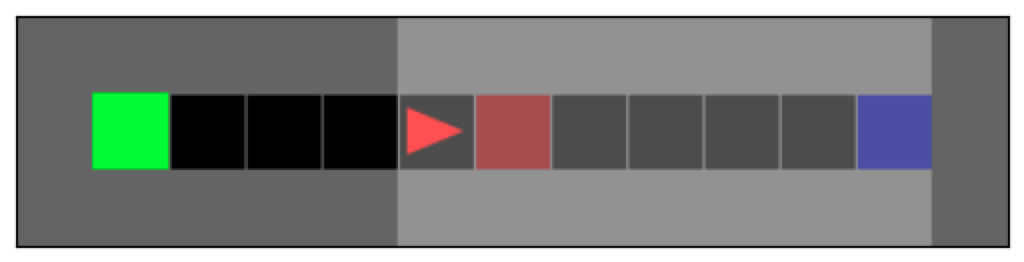
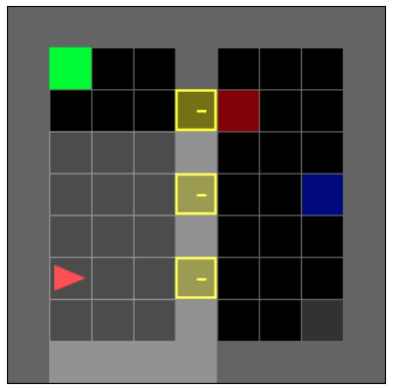
Figure 5: The Traffic Light (left) and Kitchen (right) tasks implemented in MiniGrid.

Task Descriptions:   We encode the Traffic Light and Kitchen tasks as MiniGrid environments, as shown in Figure 5. In the Traffic Light domain, the goal is to collect a package at the end of the road (represented by a blue square), and then return home (represented by the green square) without crossing a red light. The light colour stays green for a random duration, becomes yellow for one timestep, and then stays red for a random duration before returning to green. The agent can only observe squares ahead of itself, so the only safe way to cross the intersection is to check that the light is green before proceeding (at worst, the light becomes yellow while in the intersection, which is considered safe).

We introduce propositions to determine if the agent is at the package, if the agent is at home, and if the agent is in the intersection during a red light. The RM state captures two pieces of information: whether the agent has crossed a red light at any time, and whether the agent has picked up the package. Reaching the package for the first time always yields a reward of 1. Returning home with the package ends the episode and yields another reward of 1. However, if the agent has crossed a red light, it instead receives a traffic ticket in the mail (and a -1 reward).

In the Kitchen domain, the agent must enter the kitchen, perform a set of chores (represented by the coloured squares in the right room, which turn gray when finished) by visiting them, before returning to the charging port at the top left. At the start, some chores may not need the agent’s attention (e.g., if there are no dirty dishes) and that dish is considered done from the start. This occurs with a 1/3 probability for each chore, but the agent initially cannot observe which chores are done while outside the kitchen.

Propositions for each chore determine on each timestep whether that chore is currently considered done, and an additional proposition determines if the agent is at the charging port. The RM for this task captures the subset of chores completed, resulting in $9$ possible RM states (including an additional terminal state for returning to the charging port). Returning to the charging port ends the episode, giving a reward of 1 if all chores are complete and 0 otherwise. We also introduce an energy cost of -0.05 for opening the kitchen door and performing each chore (including if it’s already done, e.g. if the agent rewashes clean dishes) so that the agent must make careful decisions.

Policy Architectures:   Perfect RM, Independent Belief Updating, Thresholding, and RMSM each learned a policy conditioned on the current observation $o_{t}$ and a belief estimate of the RM state $\tilde{u}_{t}$ (or the ground-truth RM state, in the case of Perfect RM). We chose to condition policies on $o_{t}$ rather than the full history $o_{0},a_{0},\ldots,o_{t-1},a_{t-1},o_{t}$ to ensure that policies depended on the estimate $\tilde{u}_{t}$ to capture any relevant information from previous states.

Each policy consisted of the following components. Observations $o_{t}$ were encoded by a 16-channel convolutional layer, a max pooling layer, a 32-channel convolutional layer, and a 64-channel convolutional layer, in that order, each with kernel size $2\times 2$ and stride $1$. Encoded observations and the belief over RM states $\tilde{u}_{t}$ were passed into an actor head with 3 hidden layers of $64$ units and ReLU activations, and a critic head with 2 hidden layers of 64 units and tanh activations.

Recurrent PPO used a similar architecture, except the history of observations were passed through an LSTM with hidden size 64.

RM State Belief Prediction Architectures:   Independent Belief Updating and Thresholding each learned an approximation of the labelling function $\hat{\mathcal{L}}$ by predicting $|\mathcal{AP}|$ logits (representing the probabilities of each binary proposition) conditioned on the history of observations. Observations were encoded by a similar architecture as in the policy, except the final output channel was 16. The sequence of observation encodings were passed into an LSTM with hidden size 16. Final predictions were decoded from the LSTM embedding using a single hidden layer of size 16. The predicted probabilities of propositions were used to derive estimates or beliefs over RM states, as outlined in Section 4.

RMSM used the same architecture as the approximate labelling function above, except the predicted outputs were $|U|$ logits, representing a Categorical distribution over $|U|$ reward machine states.

Hyperparameters:   All policies were trained using PPO (Schulman et al. [2017]) for a total of 25 million frames in Traffic Light and 10 million frames in Kitchen. Hyperparameters are reported in Table 1. For Recurrent PPO, the number of LSTM backpropagation steps was 4.

Table 1: Hyperparameters for deep RL experiments

PPO Hyperparameters	Traffic Light	Kitchen
Env. steps per update	16384	16384
Number of epochs	8	8
Minibatch size	256	256
Discount factor ($\gamma$)	0.97	0.99
Learning rate	$3\times 10^{-4}$	$3\times 10^{-4}$
GAE-$\lambda$	0.95	0.95
Entropy coefficient	0.01	0.01
Value loss coefficient	0.5	0.5
Gradient Clipping	0.5	0.5
PPO Clipping ($\varepsilon$)	0.2	0.2
$\hat{\mathcal{L}},g_{\phi}$ Hyperparameters (if applicable)
Env. steps per update	16384	16384
Number of epochs	16	8
Minibatch size	2048	256
Learning rate	$3\times 10^{-4}$	$3\times 10^{-4}$
LSTM Backpropagation Steps	4	4

Handcrafted RM State Belief:   In Section 6.2, we compared the RM state beliefs of RMSM, Independent Belief Updating, and Thresholding against a handcrafted approximation of the true RM state belief. Note that the ground-truth RM state belief can be difficult to determine exactly.

Our approximation in Traffic Light works as follows. Propositions for collecting the package and returning home can always be determined with certainty. When crossing the intersection, we sometimes know the light colour with certainty (e.g. if the agent observed the light was green on the previous timestep, it cannot be red this timestep). We consider all other crossings of the intersection "dangerous", where the light colour is uncertain. We approximate all "dangerous" crossings to have a $0.36$ probability of occurring during a red light, the steady-state probability of the light being red after sufficient time, absent any other knowledge. Using this model of the propositions, we determine an approximate belief of the current RM state given a history.

For Kitchen, the agent has no information regarding whether each chore is initially complete while outside the kitchen. The belief over RM states during this period is easily determined using the known prior probabilities of each chore being complete. Once the agent enters the kitchen, we assume the RM state is known with certainty. Note that while this is often the case, the agent may sometimes enter the kitchen without looking at the state of all chores. We again use this model of the propositions to derive an approximate belief of the current RM state given a history.

Figure 6: The accuracy of RM state beliefs learned by RMSM, Thresholding, and Independent Belief Updating compared against a handcrafted approximation of the ground-truth RM state belief. Beliefs are conditioned on a history generated by a random policy. We report the Total Variation Distance between the predicted and (approximate) ground-truth beliefs, averaged over 8 seeds, 5 episodes per seed, and all possible histories in that episode. Error bars report standard error.

References

- Aksaray et al. (2016) Derya Aksaray, Austin Jones, Zhaodan Kong, Mac Schwager, and Calin Belta. Q-learning for Robust Satisfaction of Signal Temporal Logic Specifications. In Proceedings of the 55th IEEE Conference on on Decision and Control (CDC), pages 6565–6570. IEEE, 2016.
- Andreas et al. (2017) Jacob Andreas, Dan Klein, and Sergey Levine. Modular Multitask Reinforcement Learning with Policy Sketches. In Proceedings of the 34th International Conference on Machine Learning (ICML), pages 166–175, 2017.
- Bellman (1957) Richard Bellman. A Markovian Decision Process. Journal of Mathematics and Mechanics, pages 679–684, 1957.
- Cai et al. (2021) Mingyu Cai, Shaoping Xiao, Baoluo Li, Zhiliang Li, and Zhen Kan. Reinforcement Learning Based Temporal Logic Control with Maximum Probabilistic Satisfaction. In 2021 IEEE International Conference on Robotics and Automation (ICRA), pages 806–812. IEEE, 2021.
- Camacho et al. (2019) Alberto Camacho, Rodrigo Toro Icarte, Toryn Q. Klassen, Richard Valenzano, and Sheila A. McIlraith. LTL and Beyond: Formal Languages for Reward Function Specification in Reinforcement Learning. In Proceedings of the 28th International Joint Conference on Artificial Intelligence (IJCAI), pages 6065–6073, 2019.
- Camacho et al. (2021) Alberto Camacho, Jacob Varley, Andy Zeng, Deepali Jain, Atil Iscen, and Dmitry Kalashnikov. Reward Machines for Vision-Based Robotic Manipulation. In Proceedings of the 2021 IEEE International Conference on Robotics and Automation (ICRA), pages 14284–14290, 2021.
- Corazza et al. (2022) Jan Corazza, Ivan Gavran, and Daniel Neider. Reinforcement Learning with Stochastic Reward Machines. In Proceedings of the AAAI Conference on Artificial Intelligence, volume 36, pages 6429–6436, 2022.
- da Silva et al. (2019) Rafael Rodrigues da Silva, Vince Kurtz, and Hai Lin. Active Perception and Control from Temporal Logic Specifications. IEEE Control Systems Letters, 3(4):1068–1073, 2019.
- de Giacomo et al. (2020) Giuseppe de Giacomo, Marco Favorito, Luca Iocchi, Fabio Patrizi, and Alessandro Ronca. Temporal Logic Monitoring Rewards via Transducers. In Proceedings of the 17th International Conference on Knowledge Representation and Reasoning (KR), volume 17, pages 860–870, 2020.
- DeFazio and Zhang (2021) David DeFazio and Shiqi Zhang. Learning Quadruped Locomotion Policies with Reward Machines. arXiv preprint arXiv:2107.10969, 2021.
- Ding et al. (2011) Xu Chu Dennis Ding, Stephen L Smith, Calin Belta, and Daniela Rus. LTL Control in Uncertain Environments with Probabilistic Satisfaction Guarantees. IFAC Proceedings Volumes, 44(1):3515–3520, 2011.
- Furelos-Blanco et al. (2020) Daniel Furelos-Blanco, Mark Law, Alessandra Russo, Krysia Broda, and Anders Jonsson. Induction of Subgoal Automata for Reinforcement Learning. In Proceedings of the 34th AAAI Conference on Artificial Intelligence (AAAI), pages 3890–3897, 2020.
- Gaon and Brafman (2020) Maor Gaon and Ronen Brafman. Reinforcement Learning with non-Markovian Rewards. In Proceedings of the 34th AAAI Conference on Artificial Intelligence (AAAI), pages 3980–3987, 2020.
- Ghasemi et al. (2020) Mahsa Ghasemi, Erdem Arinc Bulgur, and Ufuk Topcu. Task-Oriented Active Perception and Planning in Environments with Partially Known Semantics. In Proceedings of the 37th International Conference on Machine Learning (ICML), 2020.
- Hasanbeig et al. (2018) Mohammadhosein Hasanbeig, Alessandro Abate, and Daniel Kroening. Logically-Constrained Reinforcement Learning. arXiv preprint arXiv:1801.08099, 2018.
- Hasanbeig et al. (2020) Mohammadhosein Hasanbeig, Daniel Kroening, and Alessandro Abate. Deep Reinforcement Learning with Temporal Logics. In Proceedings of the 18th International Conference on Formal Modeling and Analysis of Timed Systems (FORMATS), pages 1–22, 2020.
- Hopcroft et al. (2007) John E. Hopcroft, Rajeev Motwani, and Jeffrey D. Ullman. Introduction to Automata Theory, Languages, and Computation, 3rd Edition. Pearson international edition. Addison-Wesley, 2007.
- Huang et al. (2022) Wenlong Huang, Pieter Abbeel, Deepak Pathak, and Igor Mordatch. Language Models as Zero-Shot Planners: Extracting Actionable Knowledge for Embodied Agents. arXiv preprint arXiv:2201.07207, 2022.
- Jiang et al. (2019) Yiding Jiang, Shixiang Shane Gu, Kevin P Murphy, and Chelsea Finn. Language as an Abstraction for Hierarchical Deep Reinforcement Learning. Advances in Neural Information Processing Systems, 32, 2019.
- Jiang et al. (2021) Yuqian Jiang, Suda Bharadwaj, Bo Wu, Rishi Shah, Ufuk Topcu, and Peter Stone. Temporal-Logic-Based Reward Shaping for Continuing Reinforcement Learning Tasks. In Proceedings of the 35th AAAI Conference on Artificial Intelligence (AAAI), pages 7995–8003, 2021.
- Jones et al. (2013) Austin Jones, Mac Schwager, and Calin Belta. Distribution Temporal Logic: Combining Correctness with Quality of Estimation. In 52nd IEEE Conference on Decision and Control, pages 4719–4724. IEEE, 2013.
- Jothimurugan et al. (2019) Kishor Jothimurugan, Rajeev Alur, and Osbert Bastani. A Composable Specification Language for Reinforcement Learning Tasks. In Proceedings of the 33nd Conference on Advances in Neural Information Processing Systems (NeurIPS), volume 32, pages 13041–13051, 2019.
- Jothimurugan et al. (2021) Kishor Jothimurugan, Suguman Bansal, Osbert Bastani, and Rajeev Alur. Compositional Reinforcement Learning from Logical Specifications. Advances in Neural Information Processing Systems, 34:10026–10039, 2021.
- Kuo et al. (2020) Yen-Ling Kuo, Boris Katz, and Andrei Barbu. Encoding Formulas as Deep Networks: Reinforcement Learning for Zero-Shot Execution of LTL Formulas. In 2020 IEEE/RSJ International Conference on Intelligent Robots and Systems (IROS), pages 5604–5610. IEEE, 2020.
- León et al. (2020) Borja G León, Murray Shanahan, and Francesco Belardinelli. Systematic Generalisation through Task Temporal Logic and Deep Reinforcement Learning. arXiv preprint arXiv:2006.08767, 2020.
- León et al. (2022) Borja G León, Murray Shanahan, and Francesco Belardinelli. In a Nutshell, the Human Asked for This: Latent Goals for Following Temporal Specifications. In Proceedings of the 10th International Conference on Learning Representations (ICLR), 2022.
- Li et al. (2017) Xiao Li, Cristian Ioan Vasile, and Calin Belta. Reinforcement Learning with Temporal Logic Rewards. In Proceedings of the 2017 IEEE/RSJ International Conference on Intelligent Robots and Systems (IROS), pages 3834–3839, 2017.
- Li et al. (2018) Xiao Li, Yao Ma, and Calin Belta. A Policy Search Method for Temporal Logic Specified Reinforcement Learning Tasks. In Proceedings of the 2018 Annual American Control Conference (ACC), pages 240–245. IEEE, 2018.
- Littman et al. (2017) Michael L Littman, Ufuk Topcu, Jie Fu, Charles Isbell, Min Wen, and James MacGlashan. Environment-Independent Task Specifications via GLTL. arXiv preprint arXiv:1704.04341, 2017.
- Liu et al. (2022) Jason Xinyu Liu, Ankit Shah, Eric Rosen, George Konidaris, and Stefanie Tellex. Skill Transfer for Temporally-Extended Task Specifications. arXiv preprint arXiv:2206.05096, 2022.
- Luketina et al. (2019) Jelena Luketina, Nantas Nardelli, Gregory Farquhar, Jakob Foerster, Jacob Andreas, Edward Grefenstette, Shimon Whiteson, and Tim Rocktäschel. A Survey of Reinforcement Learning Informed by Natural Language. In Proceedings of the Twenty-Eighth International Joint Conference on Artificial Intelligence, IJCAI-19, pages 6309–6317. International Joint Conferences on Artificial Intelligence Organization, 7 2019. doi: 10.24963/ijcai.2019/880.
- Melo and Ribeiro (2007) Francisco S Melo and M Isabel Ribeiro. Q-learning with linear function approximation. In International Conference on Computational Learning Theory, pages 308–322. Springer, 2007.
- Neary et al. (2021) Cyrus Neary, Zhe Xu, Bo Wu, and Ufuk Topcu. Reward Machines for Cooperative Multi-Agent Reinforcement Learning. In Proceedings of the 20th International Conference on Autonomous Agents and Multiagent Systems (AAMAS), pages 934–942, 2021.
- Oh et al. (2017) Junhyuk Oh, Satinder Singh, Honglak Lee, and Pushmeet Kohli. Zero-shot Task Generalization with Multi-Task Deep Reinforcement Learning. In International Conference on Machine Learning, pages 2661–2670. PMLR, 2017.
- Rens and Raskin (2020) Gavin Rens and Jean-François Raskin. Learning non-Markovian Reward Models in MDPs. arXiv preprint arXiv:2001.09293, 2020.
- Sadigh and Kapoor (2016) Dorsa Sadigh and Ashish Kapoor. Safe Control under Uncertainty with Probabilistic Signal Temporal Logic. In Proceedings of Robotics: Science and Systems XII, 2016.
- Schulman et al. (2017) John Schulman, Filip Wolski, Prafulla Dhariwal, Alec Radford, and Oleg Klimov. Proximal Policy Optimization Algorithms. arXiv preprint arXiv:1707.06347, 2017.
- Shah et al. (2020) Ankit Shah, Shen Li, and Julie Shah. Planning with Uncertain Specifications (PUnS). IEEE Robotics and Automation Letters, 5(2):3414–3421, 2020.
- Sutton and Barto (2018) Richard S. Sutton and Andrew G. Barto. Reinforcement Learning: An Introduction. MIT press, second edition, 2018.
- Toro Icarte et al. (2018) Rodrigo Toro Icarte, Toryn Q. Klassen, Richard Valenzano, and Sheila A. McIlraith. Using Reward Machines for High-Level Task Specification and Decomposition in Reinforcement Learning. In Proceedings of the 35th International Conference on Machine Learning (ICML), pages 2107–2116, 2018.
- Toro Icarte et al. (2019) Rodrigo Toro Icarte, Ethan Waldie, Toryn Q. Klassen, Rick Valenzano, Margarita P. Castro, and Sheila A. McIlraith. Learning Reward Machines for Partially Observable Reinforcement Learning. In Proceedings of the 33nd Conference on Advances in Neural Information Processing Systems (NeurIPS), pages 15497–15508, 2019.
- Toro Icarte et al. (2022) Rodrigo Toro Icarte, Toryn Q. Klassen, Richard Valenzano, and Sheila A. McIlraith. Reward Machines: Exploiting Reward Function Structure in Reinforcement Learning. Journal of Artificial Intelligence Research, 73:173–208, 2022.
- Tuli et al. (2022) Mathieu Tuli, Andrew C. Li, Pashootan Vaezipoor, Toryn Q. Klassen, Scott Sanner, and Sheila A. McIlraith. Learning to Follow Instructions in Text-Based Games. In Proceedings of the 36rd Conference on Advances in Neural Information Processing Systems (NeurIPS), 2022. (To appear.).
- Vaezipoor et al. (2021) Pashootan Vaezipoor, Andrew Li, Rodrigo Toro Icarte, and Sheila McIlraith. LTL2Action: Generalizing LTL Instructions for Multi-Task RL. In Proceedings of the 38th International Conference on Machine Learning (ICML), pages 10497–10508, 2021.
- Velasquez et al. (2021) Alvaro Velasquez, Andre Beckus, Taylor Dohmen, Ashutosh Trivedi, Noah Topper, and George Atia. Learning Probabilistic Reward Machines from Non-Markovian Stochastic Reward Processes. CoRR, abs/2107.04633, 2021. URL http://arxiv.org/abs/2107.04633.
- Verginis et al. (2022) Christos Verginis, Cevahir Koprulu, Sandeep Chinchali, and Ufuk Topcu. Joint Learning of Reward Machines and Policies in Environments with Partially Known Semantics. arXiv preprint arXiv:2204.11833, 2022.
- Xu and Topcu (2019) Zhe Xu and Ufuk Topcu. Transfer of Temporal Logic Formulas in Reinforcement Learning. In Proceedings of the 28th International Joint Conference on Artificial Intelligence (IJCAI), pages 4010–4018, 2019.
- Xu et al. (2020) Zhe Xu, Ivan Gavran, Yousef Ahmad, Rupak Majumdar, Daniel Neider, Ufuk Topcu, and Bo Wu. Joint Inference of Reward Machines and Policies for Reinforcement Learning. In Proceedings of the 30th International Conference on Automated Planning and Scheduling (ICAPS), volume 30, pages 590–598, 2020.
- Xu et al. (2021) Zhe Xu, Bo Wu, Aditya Ojha, Daniel Neider, and Ufuk Topcu. Active Finite Reward Automaton Inference and Reinforcement Learning using Queries and Counterexamples. In International Cross-Domain Conference for Machine Learning and Knowledge Extraction, pages 115–135. Springer, 2021.
- Yuan et al. (2019) Lim Zun Yuan, Mohammadhosein Hasanbeig, Alessandro Abate, and Daniel Kroening. Modular Deep Reinforcement Learning with Temporal Logic Specifications. arXiv preprint arXiv:1909.11591, 2019.
- Zheng et al. (2022) Xuejing Zheng, Chao Yu, and Minjie Zhang. Lifelong Reinforcement Learning with Temporal Logic Formulas and Reward Machines. Knowledge-Based Systems, 257:109650, 2022.